Embed Size (px)
Citation preview

Practical CVA and KVA Forum London, 24th - 26th April 2017
Reasons behind FVA, MVA, KVA Tommaso Gabbriellini Andrea Gigli Head of Quants Head of Fixed Income and XVA
MPS Capital Services MPS Capital Services
Disclaimer _______________________________________________________________________________________________________
These are presentation slides only. The information contained herein is for general guidance on matters of interest only and
does not constitute definitive advice nor is intended to be comprehensive.
All information and opinions included in this presentation are made as of the date of this presentation.
While every attempt has been made to ensure the accuracy of the information contained herein and such information has been
obtained from sources deemed to be reliable, neither MPS Capital Services, related entities or the directors, officers
and/or employees thereof (jointly, “MPSCS") is responsible for any errors or omissions, or for the results obtained from the use
of this information. All information in this presentation is provided "as is", with no guarantee of completeness, accuracy,
timeliness or of the results obtained from the use of this information, and without warranty of any kind, express or implied,
including, but not limited to warranties of fitness for a particular purpose. MPSCS does not assume any obligation whatsoever to
communicate any changes to this document or to update its contents. In no event will MPSCS be liable to you or anyone else for
any decision made or action taken in reliance on the information in this presentation or for any consequential, special or similar
damages, even if advised of the possibility of such damages.
This document represents the views of the authors alone, and not the views of MPSCS. You can use it at your own risk.
3
Goals of the talk
• Using a multiperiodal structured model we are going to investigate
the rationale behind FVA, MVA and KVA
• The model represents a useful tool to understand the relations
between valuation adjustments, market parameters and regulatory
constraints
• Three main lessons can be learned from the model
• How to allocate capital to different business units
• How to manage funding strategies
• Hot to price banking products
4
FVA, MVA, KVA
• MVA & FVA measure the impact on Equity due to IM and VM bank’s
obligations after entering derivatives contract, using debt to finance
those obligations.
• Regulatory requirements impose that the leverage of the balance
sheet remains below a predefined threshold KVA measures the
impact on the Equity as the bank fulfils the regulatory constraints
• In order to compensate shareholders for negative variations in the
Equity value a charge equal to MVA, FVA, KVA might be needed.
5
The Model – Uniperiodal case
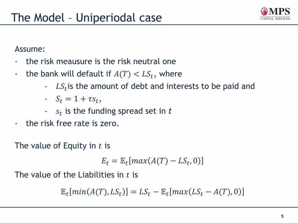
Assume:
- the risk meausure is the risk neutral one
- the bank will default if 𝐴(𝑇) < 𝐿𝑆𝑡, where
- 𝐿𝑆𝑡is the amount of debt and interests to be paid and
- 𝑆𝑡 = 1 + 𝜏𝑠𝑡,
- 𝑠𝑡 is the funding spread set in t
- the risk free rate is zero.
The value of Equity in 𝑡 is
𝐸𝑡 = 𝔼𝑡 𝑚𝑎𝑥 𝐴(𝑇) − 𝐿𝑆𝑡 , 0
The value of the Liabilities in 𝑡 is
𝔼𝑡 𝑚𝑖𝑛 𝐴(𝑇), 𝐿𝑆𝑡 = 𝐿𝑆𝑡 − 𝔼𝑡 𝑚𝑎𝑥 𝐿𝑆𝑡 − 𝐴(𝑇), 0
6
The Model – Uniperiodal case
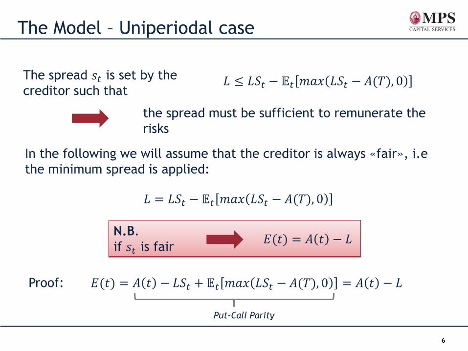
The spread 𝑠𝑡 is set by the
creditor such that 𝐿 ≤ 𝐿𝑆𝑡 − 𝔼𝑡 𝑚𝑎𝑥 𝐿𝑆𝑡 − 𝐴(𝑇), 0
the spread must be sufficient to remunerate the
risks
In the following we will assume that the creditor is always «fair», i.e
the minimum spread is applied:
𝐿 = 𝐿𝑆𝑡 − 𝔼𝑡 𝑚𝑎𝑥 𝐿𝑆𝑡 − 𝐴(𝑇), 0
N.B.
if 𝑠𝑡 is fair 𝐸(𝑡) = 𝐴 𝑡 − 𝐿
Proof: 𝐸(𝑡) = 𝐴 𝑡 − 𝐿𝑆𝑡 + 𝔼𝑡 𝑚𝑎𝑥 𝐿𝑆𝑡 − 𝐴(𝑇), 0 = 𝐴 𝑡 − 𝐿
Put-Call Parity
7
The Model – Uniperiodal case
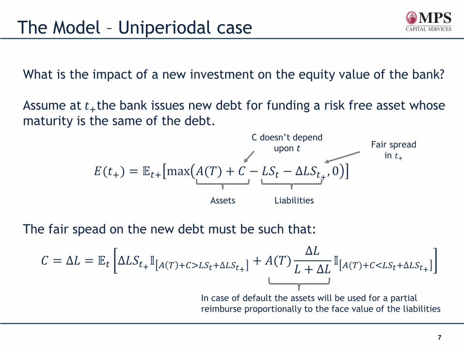
What is the impact of a new investment on the equity value of the bank?
Assume at 𝑡+the bank issues new debt for funding a risk free asset whose
maturity is the same of the debt.
The fair spead on the new debt must be such that:
Fair spread
in 𝑡+
Assets Liabilities
𝐸(𝑡+) = 𝔼𝑡+ max 𝐴(𝑇) + 𝐶 − 𝐿𝑆𝑡 − ∆𝐿𝑆𝑡+ , 0
𝐶 = ∆𝐿 = 𝔼𝑡 ∆𝐿𝑆𝑡+𝕀 𝐴 𝑇 +𝐶>𝐿𝑆𝑡+∆𝐿𝑆𝑡++ 𝐴(𝑇)
∆𝐿
𝐿 + ∆𝐿𝕀 𝐴(𝑇)+𝐶<𝐿𝑆𝑡+∆𝐿𝑆𝑡+
In case of default the assets will be used for a partial
reimburse proportionally to the face value of the liabilities
C doesn’t depend
upon t

8
The Model – Uniperiodal case
𝑇 = 𝜏 = 1
Note that:
• ∆𝐿 = 𝐶
• If 𝐴𝑡 ≫ C → 𝑆𝑡+ ≈ 𝑆𝑡
Hence, the variation in the equity value is
𝔼𝑡 max 𝐴(𝑇) + 𝐶(𝑇) − 𝐿𝑆𝑡 − ∆𝐿𝑆𝑡+, 0 − 𝔼𝑡 max 𝐴(𝑇) − 𝐿𝑆𝑡 , 0 =
≈ −𝐶 ∙ 𝝉𝑠𝑡 ∙ 𝔼𝑡 𝕀 𝐴𝑇>𝐿𝑡𝑆𝑡
This is the amount of money
shareholders requires in order to invest
borrowed money in a risk free asset
𝑡+
Assets Liabilities
𝐴(𝑡+)+ 𝐶(𝑡+)
𝐿 𝑡+ + ∆𝐿
Equity
𝔼𝑡 𝑚𝑎𝑥 𝐴(𝑇) + 𝐶 − 𝐿𝑆𝑡
− ∆𝐿𝑆𝑡+ , 0
Assets Liabilities
𝐴𝑡(𝑇)+ 𝐶
𝐿𝑆𝑡 + ∆𝐿𝑆𝑡+
Equity
𝑚𝑎𝑥 𝐴 𝑇 + 𝐶 − 𝐿𝑆𝑡
− ∆𝐿𝑆𝑡+ , 0
9
The Model – Uniperiodal case
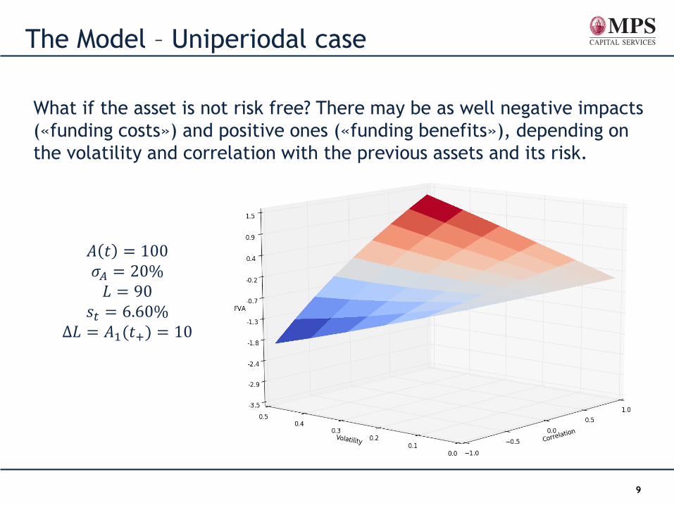
What if the asset is not risk free? There may be as well negative impacts
(«funding costs») and positive ones («funding benefits»), depending on
the volatility and correlation with the previous assets and its risk.
𝐴 𝑡 = 100
𝜎𝐴 = 20% 𝐿 = 90
𝑠𝑡 = 6.60%
Δ𝐿 = 𝐴1(𝑡+) = 10

10
The Model – Multiperiodal case
In our multiperiodal settings we assume that the bank rolls its debt at its
maturity.
For the sake of simplicity, we analyze the case where the bank rolls its
debt just once
𝜏 𝑡 2𝜏 3𝜏
𝐿 𝐿𝑆𝑡 𝐿𝑆𝑡𝑆𝜏 𝐿𝑆𝑡𝑆𝜏𝑆2𝜏
𝜏 𝑡 2𝜏
𝐿 𝐿𝑆𝑡 𝐿𝑆𝑡𝑆𝜏
11
The Model – Multiperiodal case
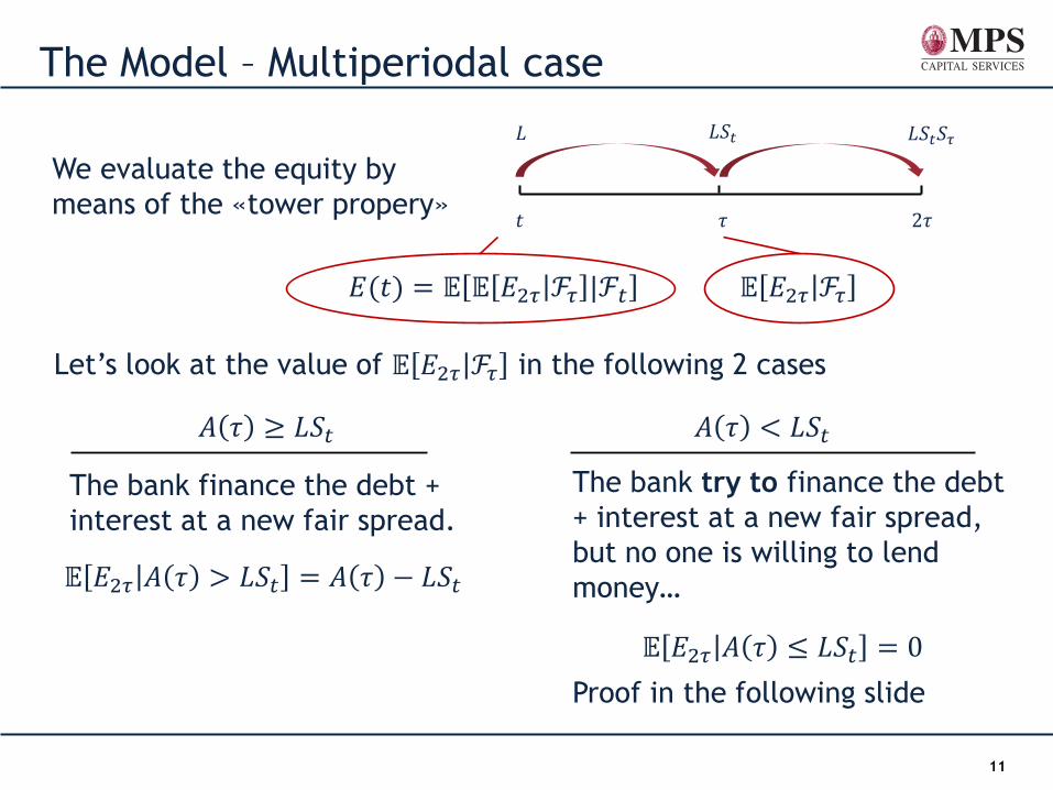
𝜏 𝑡 2𝜏
𝐿 𝐿𝑆𝑡 𝐿𝑆𝑡𝑆𝜏
We evaluate the equity by
means of the «tower propery»
𝔼 𝐸2𝜏 ℱ𝜏 𝐸(𝑡) = 𝔼 𝔼 𝐸2𝜏 ℱ𝜏 |ℱ𝑡
Let’s look at the value of 𝔼 𝐸2𝜏 ℱ𝜏 in the following 2 cases
𝐴 𝜏 ≥ 𝐿𝑆𝑡 𝐴 𝜏 < 𝐿𝑆𝑡
The bank finance the debt +
interest at a new fair spread.
𝔼 𝐸2𝜏 𝐴 𝜏 > 𝐿𝑆𝑡 = 𝐴 𝜏 − 𝐿𝑆𝑡
The bank try to finance the debt
+ interest at a new fair spread,
but no one is willing to lend
money…
𝔼 𝐸2𝜏 𝐴 𝜏 ≤ 𝐿𝑆𝑡 = 0
Proof in the following slide
12
The Model – Multiperiodal case
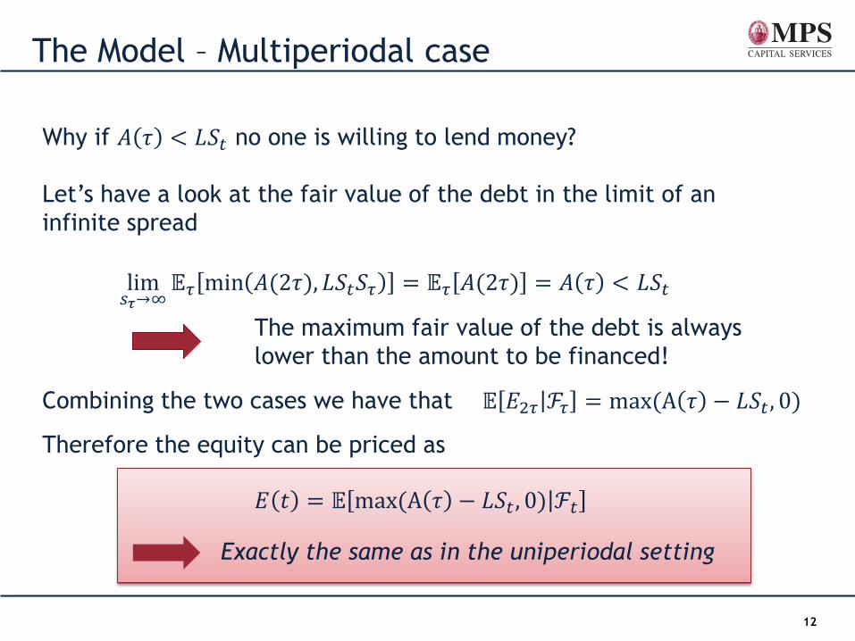
Why if 𝐴 𝜏 < 𝐿𝑆𝑡 no one is willing to lend money?
Let’s have a look at the fair value of the debt in the limit of an
infinite spread
lim𝑠𝜏→∞
𝔼𝜏 min 𝐴(2𝜏), 𝐿𝑆𝑡𝑆𝜏 = 𝔼𝜏 𝐴(2𝜏) = 𝐴 𝜏 < 𝐿𝑆𝑡
The maximum fair value of the debt is always
lower than the amount to be financed!
𝔼 𝐸2𝜏 ℱ𝜏 = max(A 𝜏 − 𝐿𝑆𝑡 , 0) Combining the two cases we have that
Therefore the equity can be priced as
𝐸 𝑡 = 𝔼 max(A 𝜏 − 𝐿𝑆𝑡, 0) ℱ𝑡
Exactly the same as in the uniperiodal setting
13
The Model – Multiperiodal case
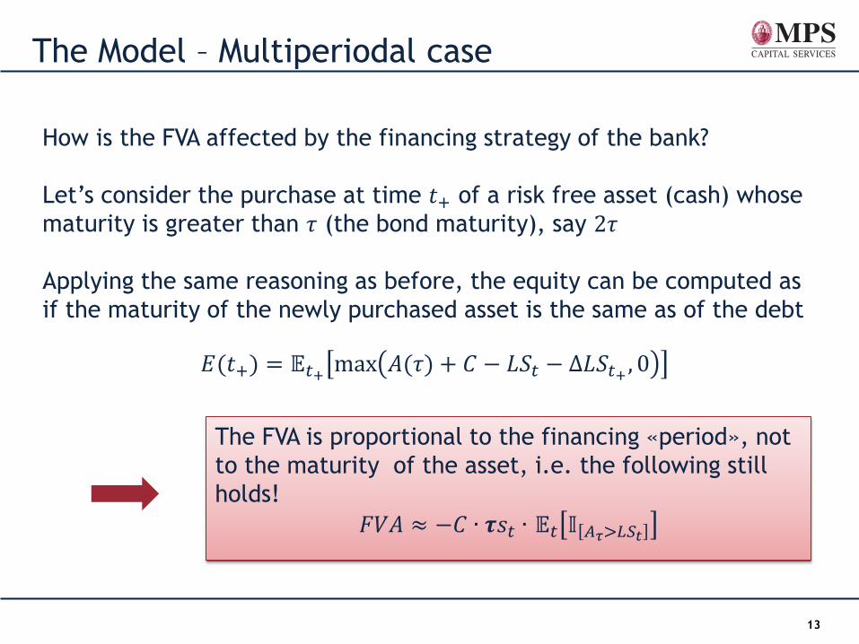
How is the FVA affected by the financing strategy of the bank?
Let’s consider the purchase at time 𝑡+ of a risk free asset (cash) whose
maturity is greater than 𝜏 (the bond maturity), say 2𝜏
Applying the same reasoning as before, the equity can be computed as
if the maturity of the newly purchased asset is the same as of the debt
𝐸(𝑡+) = 𝔼𝑡+ max 𝐴(𝜏) + 𝐶 − 𝐿𝑆𝑡 − ∆𝐿𝑆𝑡+ , 0
The FVA is proportional to the financing «period», not
to the maturity of the asset, i.e. the following still
holds!
𝐹𝑉𝐴 ≈ −𝐶 ∙ 𝝉𝑠𝑡 ∙ 𝔼𝑡 𝕀 𝐴𝜏>𝐿𝑆𝑡
14
An application for FVA/MVA
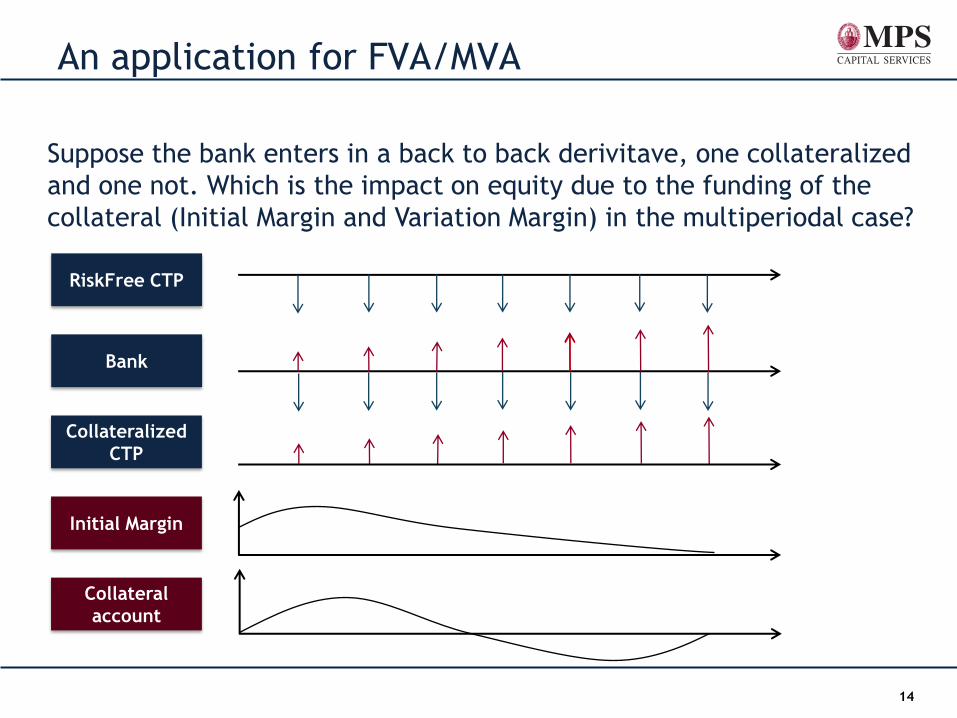
Suppose the bank enters in a back to back derivitave, one collateralized
and one not. Which is the impact on equity due to the funding of the
collateral (Initial Margin and Variation Margin) in the multiperiodal case?
RiskFree CTP
Bank
Collateralized
CTP
Initial Margin
Collateral
account
15
MVA – Uniperiodal case
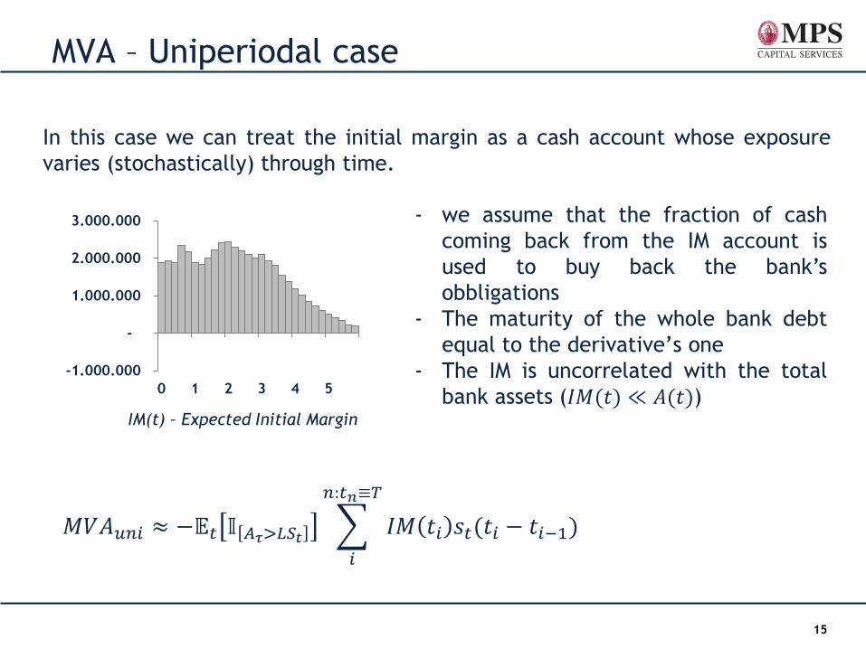
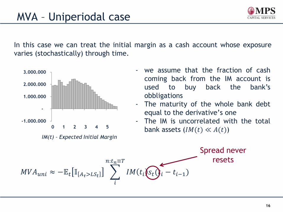
In this case we can treat the initial margin as a cash account whose exposure
varies (stochastically) through time.
-1.000.000
-
1.000.000
2.000.000
3.000.000
0 1 2 3 4 5
- we assume that the fraction of cash
coming back from the IM account is
used to buy back the bank’s
obbligations
- The maturity of the whole bank debt
equal to the derivative’s one
- The IM is uncorrelated with the total
bank assets (𝐼𝑀(𝑡) ≪ 𝐴(𝑡))
𝑀𝑉𝐴𝑢𝑛𝑖 ≈ −𝔼𝑡 𝕀 𝐴𝜏>𝐿𝑆𝑡 𝐼𝑀 𝑡𝑖 𝑠𝑡(𝑡𝑖 − 𝑡𝑖−1)
𝑛:𝑡𝑛≡𝑇
𝑖
IM(t) – Expected Initial Margin
16
MVA – Uniperiodal case
In this case we can treat the initial margin as a cash account whose exposure
varies (stochastically) through time.
-1.000.000
-
1.000.000
2.000.000
3.000.000
0 1 2 3 4 5
- we assume that the fraction of cash
coming back from the IM account is
used to buy back the bank’s
obbligations
- The maturity of the whole bank debt
equal to the derivative’s one
- The IM is uncorrelated with the total
bank assets (𝐼𝑀(𝑡) ≪ 𝐴(𝑡))
𝑀𝑉𝐴𝑢𝑛𝑖 ≈ −𝔼𝑡 𝕀 𝐴𝜏>𝐿𝑆𝑡 𝐼𝑀 𝑡𝑖 𝑠𝑡(𝑡𝑖 − 𝑡𝑖−1)
𝑛:𝑡𝑛≡𝑇
𝑖
IM(t) – Expected Initial Margin
Spread never
resets
17
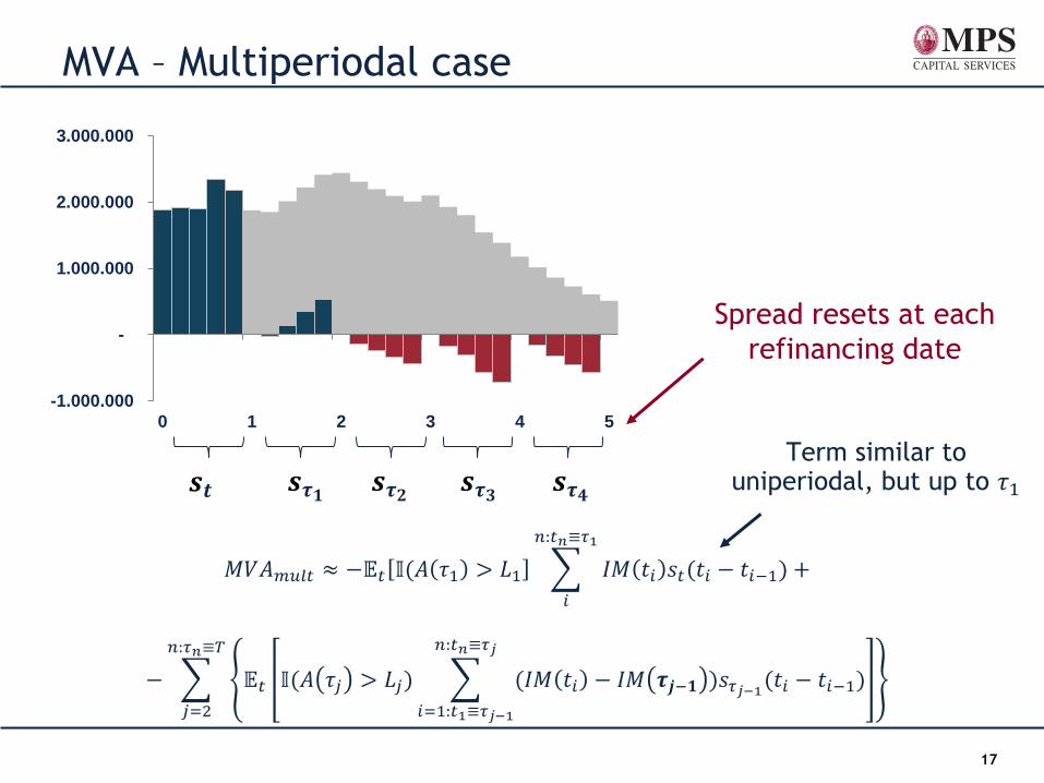
MVA – Multiperiodal case
𝑀𝑉𝐴𝑚𝑢𝑙𝑡 ≈ −𝔼𝑡 𝕀(𝐴 𝜏1 > 𝐿1 𝐼𝑀 𝑡𝑖 𝑠𝑡(𝑡𝑖 − 𝑡𝑖−1)
𝑛:𝑡𝑛≡𝜏1
𝑖
+
− 𝔼𝑡 𝕀(𝐴 𝜏𝑗 > 𝐿𝑗) (𝐼𝑀 𝑡𝑖 − 𝐼𝑀 𝝉𝒋−𝟏 )𝑠𝜏𝑗−1(𝑡𝑖 − 𝑡𝑖−1)
𝑛:𝑡𝑛≡𝜏𝑗
𝑖=1:𝑡1≡𝜏𝑗−1
𝑛:𝜏𝑛≡𝑇
𝑗=2
-1.000.000
-
1.000.000
2.000.000
3.000.000
0 1 2 3 4 5
Spread resets at each
refinancing date
Term similar to uniperiodal, but up to 𝜏1 𝒔𝒕 𝒔𝝉𝟏
𝒔𝝉𝟐 𝒔𝝉𝟑
𝒔𝝉𝟒
18
MVA – Multiperiodal case
-1.000.000
-
1.000.000
2.000.000
3.000.000
0 1 2 3 4 5
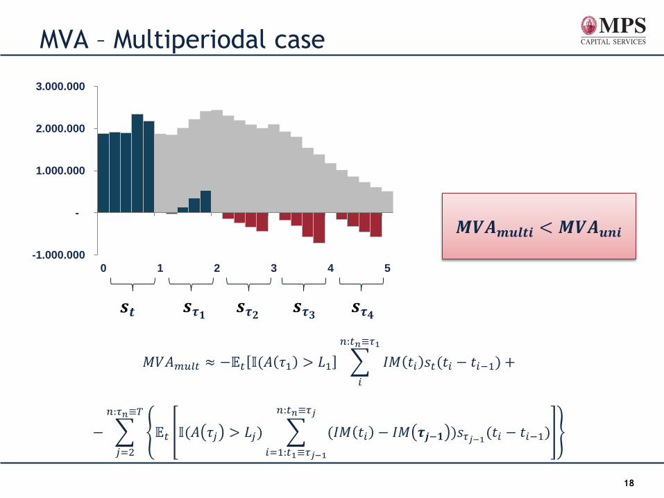
𝑴𝑽𝑨𝒎𝒖𝒍𝒕𝒊 < 𝑴𝑽𝑨𝒖𝒏𝒊
𝒔𝒕 𝒔𝝉𝟏 𝒔𝝉𝟐
𝒔𝝉𝟑 𝒔𝝉𝟒
𝑀𝑉𝐴𝑚𝑢𝑙𝑡 ≈ −𝔼𝑡 𝕀(𝐴 𝜏1 > 𝐿1 𝐼𝑀 𝑡𝑖 𝑠𝑡(𝑡𝑖 − 𝑡𝑖−1)
𝑛:𝑡𝑛≡𝜏1
𝑖
+
− 𝔼𝑡 𝕀(𝐴 𝜏𝑗 > 𝐿𝑗) (𝐼𝑀 𝑡𝑖 − 𝐼𝑀 𝝉𝒋−𝟏 )𝑠𝜏𝑗−1(𝑡𝑖 − 𝑡𝑖−1)
𝑛:𝑡𝑛≡𝜏𝑗
𝑖=1:𝑡1≡𝜏𝑗−1
𝑛:𝜏𝑛≡𝑇
𝑗=2
19
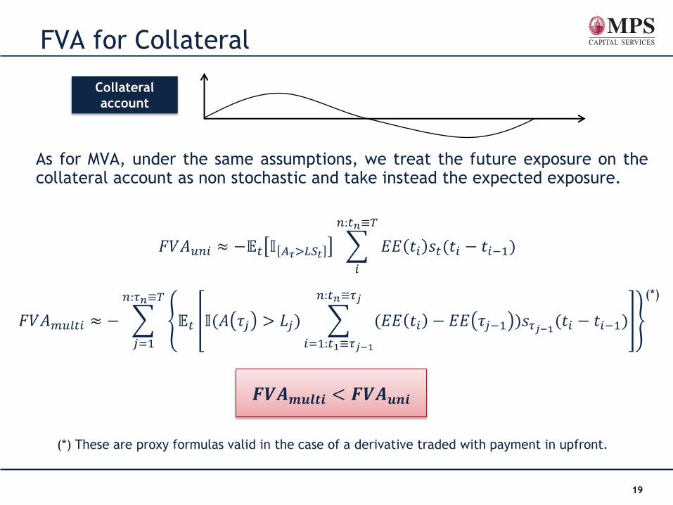
FVA for Collateral
𝐹𝑉𝐴𝑚𝑢𝑙𝑡𝑖 ≈ − 𝔼𝑡 𝕀(𝐴 𝜏𝑗 > 𝐿𝑗) (𝐸𝐸 𝑡𝑖 − 𝐸𝐸 𝜏𝑗−1 )𝑠𝜏𝑗−1(𝑡𝑖 − 𝑡𝑖−1)
𝑛:𝑡𝑛≡𝜏𝑗
𝑖=1:𝑡1≡𝜏𝑗−1
𝑛:𝜏𝑛≡𝑇
𝑗=1
Collateral
account
As for MVA, under the same assumptions, we treat the future exposure on the collateral account as non stochastic and take instead the expected exposure.
𝐹𝑉𝐴𝑢𝑛𝑖 ≈ −𝔼𝑡 𝕀 𝐴𝜏>𝐿𝑆𝑡 𝐸𝐸 𝑡𝑖 𝑠𝑡(𝑡𝑖 − 𝑡𝑖−1)
𝑛:𝑡𝑛≡𝑇
𝑖
𝑭𝑽𝑨𝒎𝒖𝒍𝒕𝒊 < 𝑭𝑽𝑨𝒖𝒏𝒊
(*)
(*) These are proxy formulas valid in the case of a derivative traded with payment in upfront.
20
KVA - Regulatory obligations
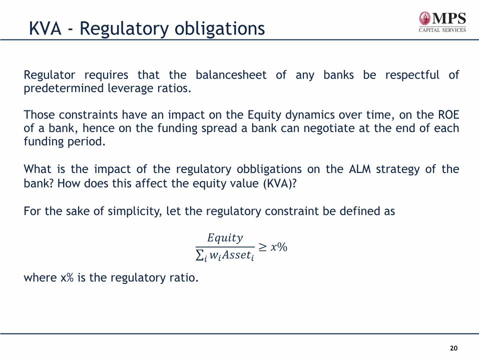
Regulator requires that the balancesheet of any banks be respectful of predetermined leverage ratios. Those constraints have an impact on the Equity dynamics over time, on the ROE of a bank, hence on the funding spread a bank can negotiate at the end of each funding period.
What is the impact of the regulatory obbligations on the ALM strategy of the
bank? How does this affect the equity value (KVA)?
For the sake of simplicity, let the regulatory constraint be defined as
𝐸𝑞𝑢𝑖𝑡𝑦
𝑤𝑖𝐴𝑠𝑠𝑒𝑡𝑖𝑖
≥ 𝑥%
where x% is the regulatory ratio.
21
A case for FVA/KVA
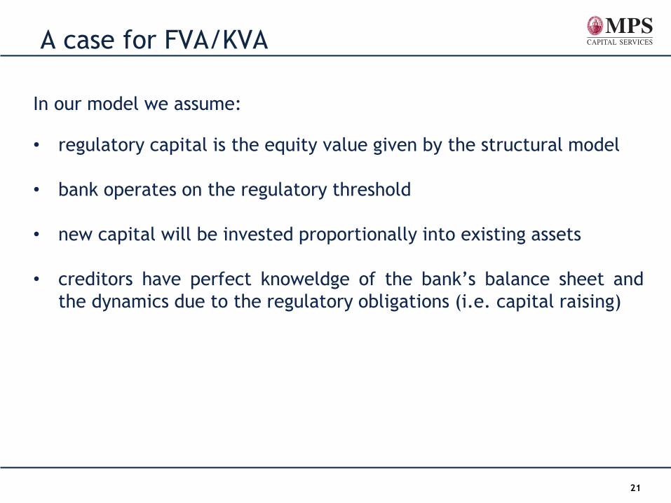
In our model we assume:
• regulatory capital is the equity value given by the structural model
• bank operates on the regulatory threshold
• new capital will be invested proportionally into existing assets
• creditors have perfect knoweldge of the bank’s balance sheet and
the dynamics due to the regulatory obligations (i.e. capital raising)
22
A case for FVA/KVA
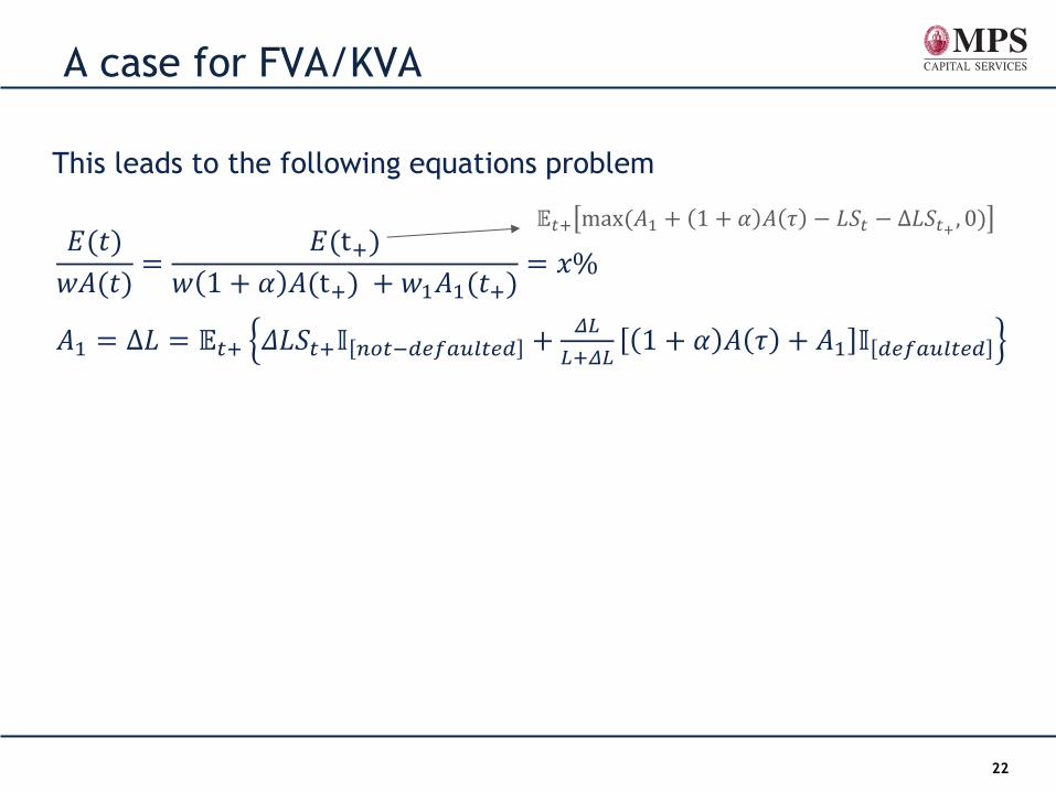
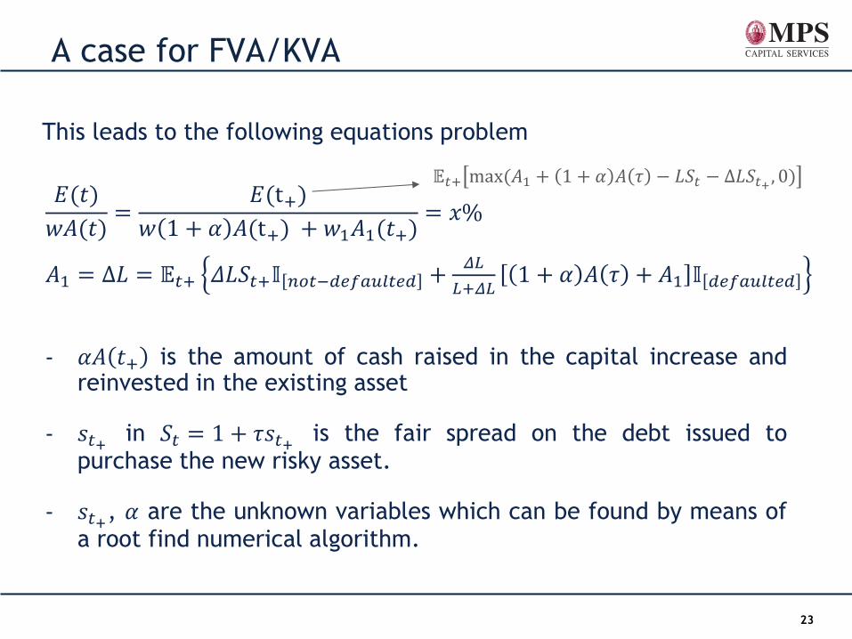
This leads to the following equations problem
𝐸(𝑡)
𝑤𝐴(𝑡)=
𝐸(t+)
𝑤 1 + 𝛼 𝐴(t+) + 𝑤1𝐴1(𝑡+)= 𝑥%
𝐴1 = Δ𝐿 = 𝔼𝑡+ 𝛥𝐿𝑆𝑡+𝕀 𝑛𝑜𝑡−𝑑𝑒𝑓𝑎𝑢𝑙𝑡𝑒𝑑 +𝛥𝐿
𝐿+𝛥𝐿1 + 𝛼 𝐴 𝜏 + 𝐴1 𝕀 𝑑𝑒𝑓𝑎𝑢𝑙𝑡𝑒𝑑
𝔼𝑡+ max (𝐴1 + 1 + 𝛼 𝐴 𝜏 − 𝐿𝑆𝑡 − Δ𝐿𝑆𝑡+ , 0)
23
A case for FVA/KVA
This leads to the following equations problem
𝐸(𝑡)
𝑤𝐴(𝑡)=
𝐸(t+)
𝑤 1 + 𝛼 𝐴(t+) + 𝑤1𝐴1(𝑡+)= 𝑥%
𝐴1 = Δ𝐿 = 𝔼𝑡+ 𝛥𝐿𝑆𝑡+𝕀 𝑛𝑜𝑡−𝑑𝑒𝑓𝑎𝑢𝑙𝑡𝑒𝑑 +𝛥𝐿
𝐿+𝛥𝐿1 + 𝛼 𝐴 𝜏 + 𝐴1 𝕀 𝑑𝑒𝑓𝑎𝑢𝑙𝑡𝑒𝑑
- 𝛼𝐴 𝑡+ is the amount of cash raised in the capital increase and reinvested in the existing asset
- 𝑠𝑡+ in 𝑆𝑡 = 1 + 𝜏𝑠𝑡+ is the fair spread on the debt issued to purchase the new risky asset.
- 𝑠𝑡+, 𝛼 are the unknown variables which can be found by means of a root find numerical algorithm.
𝔼𝑡+ max (𝐴1 + 1 + 𝛼 𝐴 𝜏 − 𝐿𝑆𝑡 − Δ𝐿𝑆𝑡+ , 0)
24
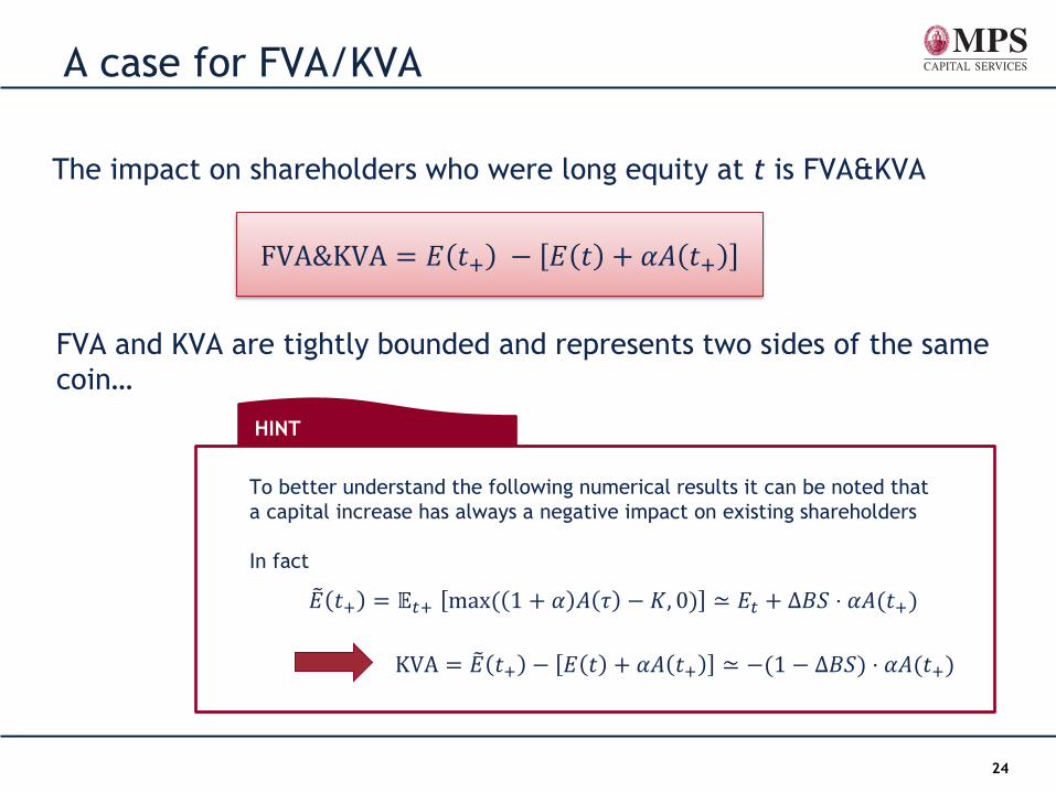
FVA and KVA are tightly bounded and represents two sides of the same
coin…
A case for FVA/KVA
The impact on shareholders who were long equity at t is FVA&KVA
FVA&KVA = 𝐸 𝑡+ − 𝐸 𝑡 + 𝛼𝐴 𝑡+
𝐸 𝑡+ = 𝔼𝑡+ max ( 1 + 𝛼 𝐴 𝜏 − 𝐾, 0) ≃ 𝐸𝑡 + Δ𝐵𝑆 ⋅ 𝛼𝐴(𝑡+)
KVA = 𝐸 𝑡+ − 𝐸 𝑡 + 𝛼𝐴 𝑡+ ≃ −(1 − Δ𝐵𝑆) ⋅ 𝛼𝐴(𝑡+)
To better understand the following numerical results it can be noted that
a capital increase has always a negative impact on existing shareholders
In fact
HINT
25
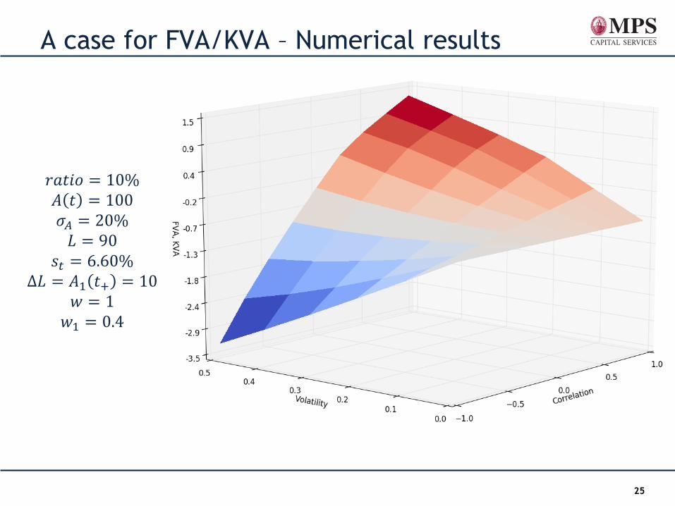
A case for FVA/KVA – Numerical results
𝑟𝑎𝑡𝑖𝑜 = 10% 𝐴 𝑡 = 100
𝜎𝐴 = 20% 𝐿 = 90
𝑠𝑡 = 6.60%
Δ𝐿 = 𝐴1 𝑡+ = 10
𝑤 = 1
𝑤1 = 0.4
26
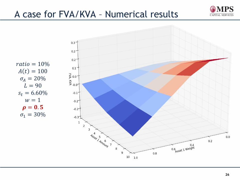
A case for FVA/KVA – Numerical results
𝑟𝑎𝑡𝑖𝑜 = 10% 𝐴 𝑡 = 100
𝜎𝐴 = 20%
𝐿 = 90
𝑠𝑡 = 6.60%
𝑤 = 1
𝝆 = 𝟎. 𝟓
𝜎1 = 30%
27
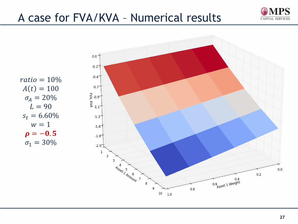
A case for FVA/KVA – Numerical results
𝑟𝑎𝑡𝑖𝑜 = 10% 𝐴 𝑡 = 100
𝜎𝐴 = 20%
𝐿 = 90
𝑠𝑡 = 6.60%
𝑤 = 1
𝝆 = −𝟎. 𝟓
𝜎1 = 30%
28
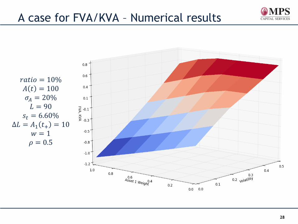
A case for FVA/KVA – Numerical results
𝑟𝑎𝑡𝑖𝑜 = 10% 𝐴 𝑡 = 100
𝜎𝐴 = 20%
𝐿 = 90
𝑠𝑡 = 6.60%
Δ𝐿 = 𝐴1 𝑡+ = 10
𝑤 = 1
𝜌 = 0.5
29
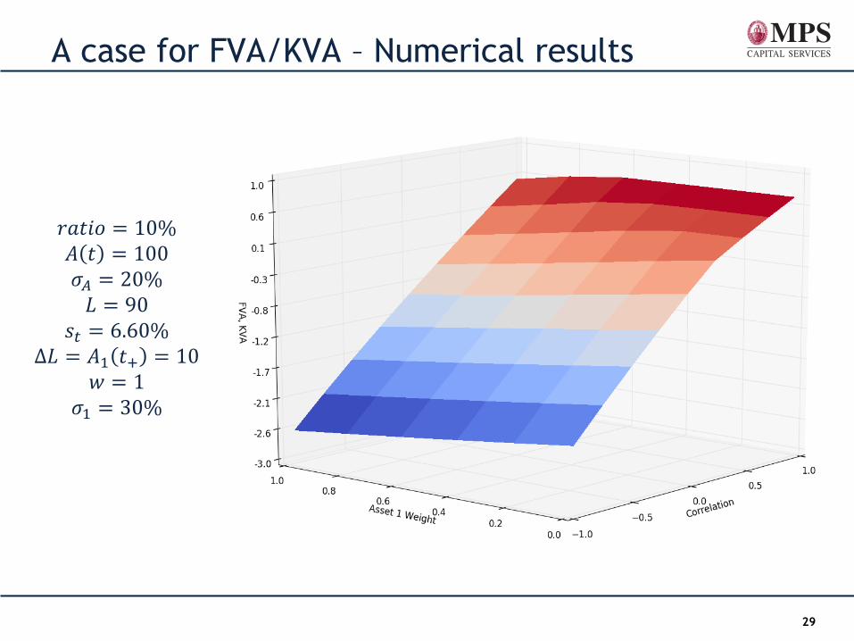
A case for FVA/KVA – Numerical results
𝑟𝑎𝑡𝑖𝑜 = 10% 𝐴 𝑡 = 100
𝜎𝐴 = 20%
𝐿 = 90
𝑠𝑡 = 6.60%
Δ𝐿 = 𝐴1 𝑡+ = 10
𝑤 = 1
𝜎1 = 30%
30
Conclusions
• We showed that the FVA and MVA impact on Equity depends on the rolling frequency of the debt and the ability of the market to price properly the funding spread at the time the debt is rolled.
• Once regulatory constraints are introduced it not possible to separate KVA and FVA components easily.
• The model defines an ALM Strategy: reduce the duration of liabilities in periods of distressed conditions and increase the duration of liabilities in period of flourishing conditions.
• The model defines the Pricing Policy: even if assets fair values do not depend on bank’s funding cost, a pricing policy should also take into account of potential losses on equity value due to funding level.
• The model defines a Transfer Price Policy: fund any business unit accordingly to the marginal contribution to the total risk of the Assets in the balance-sheet.

31
Play with the
model at
www.x-va.online

Questions?
Tommaso Gabbriellini Andrea Gigli Head of Quants Head of Fixed Income and XVAs
MPS Capital Services MPS Capital Services