Chapter 6

Non-competitive MarkNon-competitive MarkNon-competitive MarkNon-competitive MarkNon-competitive Marketsetsetsetsets

We recall that perfect competition was theorised as a marketstructure where both consumers and firms were price takers.The behaviour of the firm in such circumstances was describedin the Chapter 4. We discussed that the perfect competitionmarket structure is approximated by a market satisfying thefollowing conditions:(i) there exist a very large number of firms and consumers of the

commodity, such that the output sold by each firm is negligiblysmall compared to the total output of all the firms combined,and similarly, the amount purchased by each consumer isextremely small in comparison to the quantity purchased byall consumers together;

(ii) firms are free to start producing the commodity or to stopproduction;

(iii) the output produced by each firm in the industry isindistinguishable from the others and the output of any otherindustry cannot substitute this output; and

(iv) consumers and firms have perfect knowledge of the output,inputs and their prices.In this chapter, we shall discuss situations where one or more

of these conditions are not satisfied. If assumptions (i) and (ii) aredropped, we get market structures called monopoly and oligopoly.If assumption (iii) is dropped, we obtain a market structure calledmonopolistic competition. Dropping of assumption (iv) is dealt withas ‘economics of risk’. This chapter will examine the marketstructures of monopoly, monopolistic competition and oligopoly.

6.1 SIMPLE MONOPOLY IN THE COMMODITY MARKET

A market structure in which there is a single selleris called monopoly. The conditions hidden inthis single line definition, however, need to beexplicitly stated. A monopoly marketstructure requires that there is asingle producer of a particularcommodity; no other commodityworks as a substitute forthis commodity; and for thissituation to persist overtime, sufficient restrictions ‘I’ ‘M’ Perfect Competition

In order to examine the difference in the equilibrium resulting from a monopolyin the commodity market as compared to other market structures, we also needto assume that all other markets remain perfectly competitive. In particular, weneed (i) that the market of the particular commodity is perfectly competitivefrom the demand side ie all the consumers are price takers; and (ii) that themarkets of the inputs used in the production of this commodity are perfectlycompetitive both from the supply and demand side.

If all the above conditions are satisfied, then we define the situation as one ofmonopoly in a single commodity market.

6.1.1 Market Demand Curve is the Average Revenue Curve

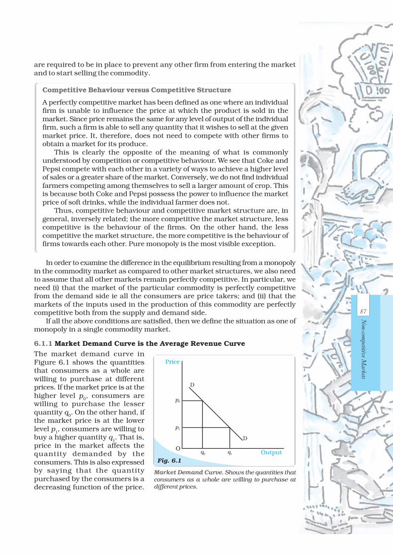
The market demand curve inFigure 6.1 shows the quantitiesthat consumers as a whole arewilling to purchase at differentprices. If the market price is at thehigher level p0, consumers arewilling to purchase the lesserquantity q0. On the other hand, ifthe market price is at the lowerlevel p1, consumers are willing tobuy a higher quantity q

1. That is,

price in the market affects thequantity demanded by theconsumers. This is also expressedby saying that the quantitypurchased by the consumers is adecreasing function of the price.

Competitive Behaviour versus Competitive Structure

A perfectly competitive market has been defined as one where an individualfirm is unable to influence the price at which the product is sold in themarket. Since price remains the same for any level of output of the individualfirm, such a firm is able to sell any quantity that it wishes to sell at the givenmarket price. It, therefore, does not need to compete with other firms toobtain a market for its produce.

This is clearly the opposite of the meaning of what is commonlyunderstood by competition or competitive behaviour. We see that Coke andPepsi compete with each other in a variety of ways to achieve a higher levelof sales or a greater share of the market. Conversely, we do not find individualfarmers competing among themselves to sell a larger amount of crop. Thisis because both Coke and Pepsi possess the power to influence the marketprice of soft drinks, while the individual farmer does not.

Thus, competitive behaviour and competitive market structure are, ingeneral, inversely related; the more competitive the market structure, lesscompetitive is the behaviour of the firms. On the other hand, the lesscompetitive the market structure, the more competitive is the behaviour offirms towards each other. Pure monopoly is the most visible exception.

Market Demand Curve. Shows the quantities thatconsumers as a whole are willing to purchase atdifferent prices.

Fig. 6.1

Price

Outputq0 q1

p0

p1

D

D

O

are required to be in place to prevent any other firm from entering the marketand to start selling the commodity.

87

Non-com

petitive Markets

88

Intr

oduc

tory

Mic

roec

onom

ics

For the monopoly firm, the above argument expresses itself from the reversedirection. The monopoly firm’s decision to sell a larger quantity is possible onlyat a lower price. Conversely, if the monopoly firm brings a smaller quantity ofthe commodity into the market for sale it will be able to sell at a higher price.Thus, for the monopoly firm, the price depends on the quantity of the commoditysold. The same is also expressed by stating that price is a decreasing function ofthe quantity sold. Thus, for the monopoly firm, the market demand curveexpresses the price that is available for different quantities supplied. This idea isreflected in the statement that the monopoly firm faces the market demand curve.

The above idea can be viewed from another angle. Since the firm is assumedto have perfect knowledge of the market demand curve, the monopoly firm candecide the price at which it wishes to sell its commodity, and therefore, determinesthe quantity to be sold. For instance, examining Figure 6.1 again, since themonopoly firm is aware of the shape of the curve DD, if it wishes to sell thecommodity at the price p

0, it can do so by producing and selling quantity q

0,

since at the price p0, consumers are willing to purchase the quantity q0. Thisidea is concretised in the slogan: ‘Monopoly firm is a price maker’.

The contrast with the firm in a perfectly competitive market structure shouldbe clear. In that case, the firm could bring into the market as much quantity ofthe commodity as it wished and could sell it at the same price. Since this doesnot happen for a monopoly firm, the amount of money received by the firmthrough the sale of the commodity has to be examined again.

We do this exercise through a schedule, a graph, and using a simple equationof a straight line demand curve. As an example, let the demand function begiven by the equation

q = 20 – 2p,

where q is the quantity sold and p is the price in rupees.The equation can be written in terms of p as

p = 10 – 0.5q

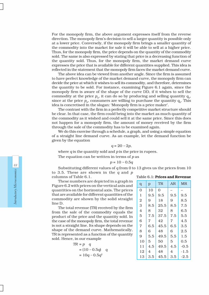
Substituting different values of q from 0 to 13 gives us the prices from 10to 3.5. These are shown in the q and pcolumns of Table 6.1.

These numbers are depicted in a graph inFigure 6.2 with prices on the vertical axis andquantities on the horizontal axis. The pricesthat are available for different quantities of thecommodity are shown by the solid straightline D.

The total revenue (TR) received by the firmfrom the sale of the commodity equals theproduct of the price and the quantity sold. Inthe case of the monopoly firm, the total revenueis not a straight line. Its shape depends on theshape of the demand curve. Mathematically,TR is represented as a function of the quantitysold. Hence, in our example

TR = p × q

= (10 – 0.5q) × q

= 10q – 0.5q2

q p TR AR MR

0 10 0 – –1 9.5 9.5 9.5 9.52 9 18 9 8.53 8.5 25.5 8.5 7.54 8 32 8 6.55 7.5 37.5 7.5 5.56 7 42 7 4.57 6.5 45.5 6.5 3.58 6 48 6 2.59 5.5 49.5 5.5 1.510 5 50 5 0.511 4.5 49.5 4.5 -0.512 4 48 4 -1.513 3.5 45.5 3.5 -2.5

Table 6.1: Prices and Revenue

89

Non-com

petitive Markets

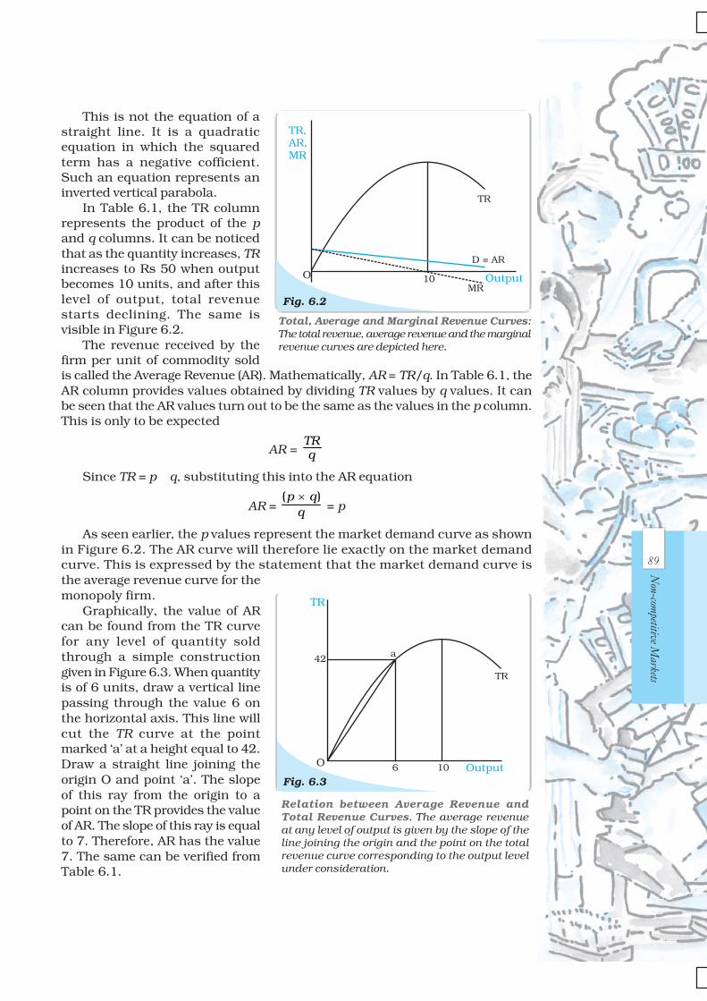
This is not the equation of astraight line. It is a quadraticequation in which the squaredterm has a negative cofficient.Such an equation represents aninverted vertical parabola.

In Table 6.1, the TR columnrepresents the product of the pand q columns. It can be noticedthat as the quantity increases, TRincreases to Rs 50 when outputbecomes 10 units, and after thislevel of output, total revenuestarts declining. The same isvisible in Figure 6.2.

The revenue received by thefirm per unit of commodity soldis called the Average Revenue (AR). Mathematically, AR = TR/q. In Table 6.1, theAR column provides values obtained by dividing TR values by q values. It canbe seen that the AR values turn out to be the same as the values in the p column.This is only to be expected

AR = TRq

Since TR = p × q, substituting this into the AR equation

AR = ( )p q

q×

= p

As seen earlier, the p values represent the market demand curve as shownin Figure 6.2. The AR curve will therefore lie exactly on the market demandcurve. This is expressed by the statement that the market demand curve isthe average revenue curve for themonopoly firm.

Graphically, the value of ARcan be found from the TR curvefor any level of quantity soldthrough a simple constructiongiven in Figure 6.3. When quantityis of 6 units, draw a vertical linepassing through the value 6 onthe horizontal axis. This line willcut the TR curve at the pointmarked ‘a’ at a height equal to 42.Draw a straight line joining theorigin O and point ‘a’. The slopeof this ray from the origin to apoint on the TR provides the valueof AR. The slope of this ray is equalto 7. Therefore, AR has the value7. The same can be verified fromTable 6.1.

Relation between Average Revenue andTotal Revenue Curves. The average revenueat any level of output is given by the slope of theline joining the origin and the point on the totalrevenue curve corresponding to the output levelunder consideration.

Total, Average and Marginal Revenue Curves:The total revenue, average revenue and the marginalrevenue curves are depicted here.

Fig. 6.2

TR,AR,MR

OutputO 10MR

D = AR

TR

90

Intr

oduc

tory

Mic

roec

onom

ics

6.1.2 Total, Average and Marginal Revenues

A more careful glance at Table 6.1 reveals that TR does not increase by thesame amount for every unit increase in quantity. Sale of the first unit leads toa change in TR from Rs 0 when quantity is of 0 unit to Rs 9.50 when quantityis 1 unit, i.e., a rise of Rs 9.50. As the quantity increases further, the rise in TRis smaller. For example, for the 5th unit of the commodity, the rise in TR isRs 5.50 (Rs 37.50 for 5 units minus Rs 32 for 4 units). As mentioned earlier,after 10 units of output, TR starts declining. This implies that bringing morethan 10 units for sale leads to a level of TR less than Rs 50. Thus, the rise in TRdue to the 12th unit is: 48 – 49.50 = –1.5, ie a fall of Rs 1.50.

This change in TR due to the sale of an additional unit is termed MarginalRevenue (MR). In Table 6.1, this is depicted in the last column. The values inevery row of the MR column after the first equal the TR value in that row minusthe TR value in the previous row. In the last paragraph, it was shown that TRincreases more slowly as quantity sold increases and falls after quantity reaches10 units. The same can be viewed through the MR values which fall as qincreases. After the quantity reaches 10 units, MR has negative values. In Figure6.2, MR is depicted by the dotted line.

Graphically, the values ofthe MR curve are given by theslope of the TR curve. The slopeof any smooth curve is definedas the slope of the tangent to thecurve at that point. This isdepicted in Figure 6.4. At point‘a’ on the TR curve, the value ofMR is given by the slope of theline L

1, and at point ‘b’ by the

line L2. It can be seen that both

lines have positive slope, but theline L

2 is flatter than line L

1, ie

its slope is lesser. The value ofMR for the same level of quantityis also lesser. When 10 units ofthe commodity are sold, thetangent to the TR is horizontal,ie its slope is zero. The value ofthe MR for the same quantity is zero. At point ‘d’ on the TR curve, where thetangent is negatively sloped, the MR takes a negative value.

We can now conclude that when total revenue is rising, marginal revenueis positive, and when total revenue shows a fall, marginal revenue is negative.

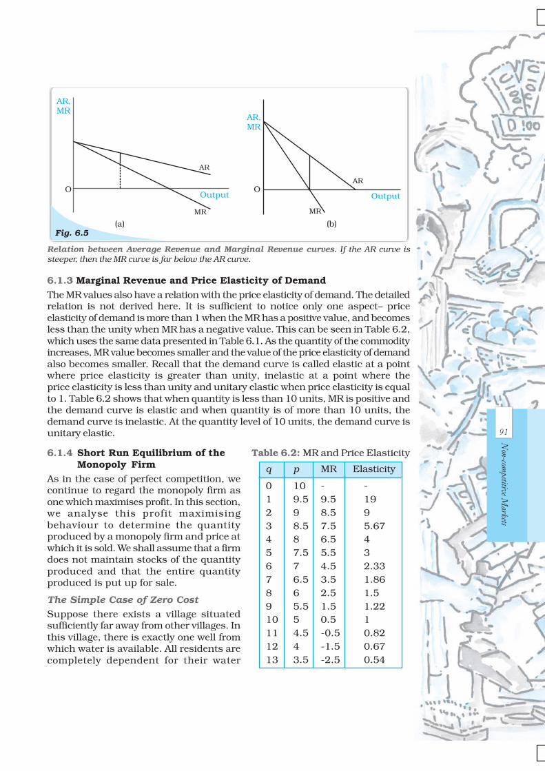
Another relation can be seen between the AR and the MR curves. Figure6.2 shows that the MR curve lies below the AR curve. The same can be seen inTable 6.1 where the values of MR at any level of output are lower than thecorresponding values of AR. We can conclude that if the AR curve (ie the demandcurve) is falling steeply, the MR curve is far below the AR curve. On the otherhand, if the AR curve is less steep, the vertical distance between the AR andMR curves is smaller. Figure 6.5(a) shows a flatter AR curve while Figure 6.5(b)shows a steeper AR curve. For the same units of the commodity, the differencebetween AR and MR in panel (a) is smaller than the difference in panel (b).

Relation between Marginal Revenue and TotalRevenue Curves. The marginal revenue at any levelof output is given by the slope of the total revenuecurve at that level of output.

Fig. 6.4

TR,MR

Output

TRb

aL1

L2

c

d

O 10MR

91

Non-com

petitive Markets

Relation between Average Revenue and Marginal Revenue curves. If the AR curve issteeper, then the MR curve is far below the AR curve.

Fig. 6.5(a)

Output

AR

MR

O

AR,MR

AR

MR

Output

AR,MR

O

(b)

6.1.3 Marginal Revenue and Price Elasticity of Demand

The MR values also have a relation with the price elasticity of demand. The detailedrelation is not derived here. It is sufficient to notice only one aspect– priceelasticity of demand is more than 1 when the MR has a positive value, and becomesless than the unity when MR has a negative value. This can be seen in Table 6.2,which uses the same data presented in Table 6.1. As the quantity of the commodityincreases, MR value becomes smaller and the value of the price elasticity of demandalso becomes smaller. Recall that the demand curve is called elastic at a pointwhere price elasticity is greater than unity, inelastic at a point where theprice elasticity is less than unity and unitary elastic when price elasticity is equalto 1. Table 6.2 shows that when quantity is less than 10 units, MR is positive andthe demand curve is elastic and when quantity is of more than 10 units, thedemand curve is inelastic. At the quantity level of 10 units, the demand curve isunitary elastic.

6.1.4 Short Run Equilibrium of theMonopoly Firm

As in the case of perfect competition, wecontinue to regard the monopoly firm asone which maximises profit. In this section,we analyse this profit maximisingbehaviour to determine the quantityproduced by a monopoly firm and price atwhich it is sold. We shall assume that a firmdoes not maintain stocks of the quantityproduced and that the entire quantityproduced is put up for sale.

The Simple Case of Zero CostSuppose there exists a village situatedsufficiently far away from other villages. Inthis village, there is exactly one well fromwhich water is available. All residents arecompletely dependent for their water

q p MR Elasticity

0 10 - -1 9.5 9.5 192 9 8.5 93 8.5 7.5 5.674 8 6.5 45 7.5 5.5 36 7 4.5 2.337 6.5 3.5 1.868 6 2.5 1.59 5.5 1.5 1.2210 5 0.5 111 4.5 -0.5 0.8212 4 -1.5 0.6713 3.5 -2.5 0.54

Table 6.2: MR and Price Elasticity

92

Intr

oduc

tory

Mic

roec

onom

ics

requirements on this well. The well is owned by one person who is able to preventothers from drawing water from it except through purchase of water. The personwho purchases the water has to draw the water out of the well. The well owner isthus a monopolist firm which bears zero cost in producing the good.We shall analyse this simple case of a monopolist bearing zero costs to determinethe amount of water sold and the price at which it is sold.

Figure 6.6 depicts the sameTR, AR and MR curves, as inFigure 6.2. The profit received bythe firm equals the revenuereceived by the firm minus the costincurred, that is, Profit = TR – TC.Since in this case TC is zero, profitis maximum when TR ismaximum. This, as we have seenearlier, occurs when output is of10 units. This is also the levelwhen MR equals zero. Theamount of profit is given by thelength of the vertical line segmentfrom ‘a’ to the horizontal axis.

The price at which this outputwill be sold is the price that theconsumers as a whole are willingto pay. This is given by the market demand curve D. At output level of 10units, the price is Rs 5. Since the market demand curve is the AR curve for themonopolist firm, Rs 5 is the average revenue received by the firm. The totalrevenue is given by the product of AR and the quantity sold, ie Rs 5 × 10 units= Rs 50. This is depicted by the area of the shaded rectangle.

Comparison with Perfect CompetitionWe compare the above outcome with what it would be under perfectly competitivemarket structure. Let us assume that there is an infinite number of such wells.If one well owner charges Rs 5 per unit of water to get a profit of Rs 50, anotherwell owner realising there are still consumers willing to buy water at a lowerrate, will fix the price lower than Rs 5, say at Rs 4. Consumers will decide topurchase from the second water seller and demand a larger quantity of 12 unitscreating a total revenue of Rs 48. In similar fashion, another water seller, inorder to obtain the revenue, would offer a still lower price, say Rs 3, and selling14 units earning a revenue of Rs 42. Since there is an infinite number of firms,price would continue to move down infinitely till it reaches zero. At this output,20 units of water would be sold and profit would become zero.

Through this comparison, we can see that a perfectly competitive equilibriumresults in a larger quantity being sold at a lower price. We can now proceed tothe general case involving positive costs of production.

Introducing Positive CostsAnalysing using Total curves

In Chapter 3, we have discussed the concept of cost and the shape of the totalcost curve having been depicted as shown by TC in Figure 6.7. The TR curve isalso drawn in the same diagram. The profit received by the firm equals the totalrevenue minus the total cost. In the figure, we can see that if quantity q

1 is

Short Run Equilibrium of the Monopolist withZero Costs. The monopolist’s profit is maximisedat that level of output for which the total revenue isthe maximum.

Fig. 6.6

OutputO 10MR

AR = D5

a

TR,AR,MR,Price

TR

93

Non-com

petitive Markets

produced, the total revenue is TR1 and total cost is TC

1. The difference, TR

1 – TC

1,

is the profit received. The same is depicted by the length of the line segment AB,i.e., the vertical distance between the TR and TC curves at q

1 level of output. It

should be clear that this vertical distance changes for diferent levels of output.When output level is less than q

2, the TC curve lies above the TR curve, i.e., TC is

greater than TR, and therefore profit is negative and the firm makes losses.The same situation exists for

output levels greater than q3.

Hence, the firm can make positiveprofits only at output levelsbetween q

2 and q

3, where TR curve

lies above the TC curve. Themonopoly firm will choose thatlevel of output which maximisesits profit. This would be the levelof output for which the verticaldistance between the TR and TCis maximum and TR is above theTC, i.e., TR – TC is maximum. Thisoccurs at the level of output q

0.

If the difference TR – TC iscalculated and drawn as a graph,it will look as in the curve marked‘Profit’ in Figure 6.7. It should benoticed that the Profit curve hasits maximum value at the level ofoutput q

0.

The price at which this output is sold is the price consumers are willing to payfor this q0 quantity of the commodity. So the monopoly firm will charge the pricecorresponding to the quantity level q0 on the demand curve.

Using Average and Marginal curves

The analysis shown above can also be conducted using Average and MarginalRevenue and Average and Marginal Cost. Though a bit more complex, thismethod is able to exhibit the process in greater light.

In Figure 6.8, the AverageCost (AC), Average Variable Cost(AVC) and Marginal Cost (MC)curves are drawn along with theDemand (Average Revenue) Curveand Marginal Revenue crve.

It may be seen that at quantitylevel below q0, the level of MR ishigher than the level of MC. Thismeans that the increase in totalrevenue from selling an extra unitof the commodity is greater thanthe increase in total cost forproducing the additional unit. Thisimplies that an additional unit ofoutput would create additionalprofits since Change in profit =Change in TR – Change in TC.

Equilibrium of the Monopolist in terms of theTotal Curves. The monopolist’s profit is maximisedat the level of output for which the vertical distancebetween the TR and TC is a maximum and TR isabove the TC.

Fig. 6.7

Rev

enu

e,C

ost,

Pro

fit

TR1

TC1

O q1 q0q2 q3 Output

Profit

A

a

B

TC

TR

Equilibrium of the Monopolist in terms of theAverage and the Marginal Curve. The monopolist’sprofit is maximised at that level of output for whichthe MR = MC and the MC is rising.

Fig. 6.8Output

Price

q0 qC

ed

af

MC

AC

b

MR

pCc

O

D = AR

94

Intr

oduc

tory

Mic

roec

onom

ics

Therefore, if the firm is producing a level of output less than q0, it would desire to

increase its output since that would add to its profits. As long as the MR curve liesabove the MC curve, the reasoning provided above would apply and thus the firmwould increase its output. This process comes to a halt when the firm reaches anoutput level of q

0 since at this level MR equals MC and increasing output provides

no increase in profits.On the other hand, if the firm was producing a level of output which is greater

than q0, MC is greater than MR. This means that the lowering of total cost by

reducing one unit of output is greater than the loss in total revenue due to thisreduction. It is therefore advisable for the firm to reduce output. This argumentwould hold good as long as the MC curve lies above the MR curve, and the firmwould keep reducing its output. Once output level reaches q

0, the values of MC

and MR become equal and the firm stops reducing its output.Since the firm inevitably reaches the output level q

0, this level is called the

equilibrium level of output. Since this equilibrium level of output correspondsto the point where the MR equals MC, this equality is called the equilibriumcondition for the output produced by a monopoly firm.

At this equilibrium level of output q0, the average cost is given by the point

‘d’ where the vertical line from q0 cuts the AC curve. The average cost is thusgiven by the height dq

0. Since total cost equals the product of AC and the quantity

produced being q0, the same is given by the area of the rectangle Oq0dc.As shown earlier, once the quantity of output produced is determined, the

price at which it is sold is given by the amount that the consumers are willing topay, as expressed through the market demand curve. Thus, the price is givenby the point ‘a’ where the vertical line through q0 meets the market demandcurve D. This provides price given by the height aq

0. Since the price received by

the firm is the revenue per unit of output, it is the Average Revenue for the firm.The total revenue being the product of AR and the level of output q

0, can be

shown as the area of the rectangle Oq0ab.It can be seen from the diagram that the area of the rectangle Oq

0ab is larger

than the area of the rectangle Oq0dc, i.e., TR is greater than TC. The difference isthe area of the rectangle cdab. Thus, Profit = TR – TC which can be representedby this area cdab.

Comparison with Perfect Competition againWe compare the monopoly firm’s equilibrium quantity and price with that ofthe perfectly competitive firm. Recall that the perfectly competitive firm was aprice taker. Given the market price, the firm in a perfectly competitive marketstructure believed that it could not alter the price by producing more of theoutput or less of it.

Suppose that the firm, whose equilibrium we were considering above, believedthat it was a perfectly competitive firm. Then, given its level of output at q

0, price

of the commodity at aq0 = Ob, it would expect the price to remain fixed at Ob,and therefore, every additional unit of output could be sold at that price. Sincethe cost of producing an additional unit, given by the MC, stands at eq0 which isless than aq

0, the firm would expect a gain in profit by increasing the output.

This would continue as long as the price remained higher than the MC. At thepoint ‘f ’ in Figure 6.8, where the MC curve cuts the demand curve, price receivedby the firm becomes equal to the MC. Hence, it would no longer be consideredbeneficial by this perfectly competitive firm to increase output. It is for this reasonthat Price = Marginal Cost that is considered the equilibrium condition for theperfectly competitive firm.

95

Non-com

petitive Markets

The diagram shows that at this level of output, the quantity produced qc is

greater than q0. Also, the price paid by the consumers is lower at pc. From this weconclude that the perfectly competitive market provides a production and sale ofa larger quantity of the commodity compared to a monopoly firm. Further theprice of the commodity under perfect competition is lower compared to monopoly.The profit earned by the perfectly competitive firm is also smaller.

In the Long RunWe saw in Chapter 5 that with free entry and exit, perfectly competitive firmsobtain zero profits. That was due to the fact that if profits earned by firms werepositive, more firms would enter the market and the increase in output wouldbring the price down, thereby decreasing the earnings of the existing firms.Similarly, if firms were facing losses, some firms would close down and thereduction in output would raise prices and increase the earnings of the remainingfirms. The same is not the case with monopoly firms. Since other firms areprevented from entering the market, the profits earned by monopoly firms donot go away in the long run.

Some Critical ViewsThe results presented above portray an extremely negative picture of the impactof monopoly in a commodity market: the monopoly firms solely benefitthemselves, at the cost of consumers. The monopoly firm receives a higherprofit and a positive profit even in the long run. On the other hand, consumersget a lesser quantity of the output and have to pay more for each unit consumed.

However, varying views have been expressed by economists concerning thequestion of monopoly. First, it can be argued that monopoly of the kind describedabove cannot exist in the real world. This is because all commodities are, in asense, substitutes for each other. This in turn is because of the fact that all thefirms producing commodities, in the final analysis, compete to obtain the incomein the hands of consumers.

Another argument is that even a firm in a pure monopoly situation is neverwithout competition. This is because the economy is never stationary. Newcommodities using new technologies are always coming up, which are closesubstitutes for the commodity produced by the monopoly firm. Hence, themonopoly firm always has competition in the long run. Even in the short run,the threat of competition is always present and the monopoly firm is unable tobehave in the manner we have described above.

Still another view argues that the existence of monopolies may be beneficialto society. Since monopoly firms earn large profits, they possess sufficient fundsto take up research and development work, something which the small perfectlycompetitive firm is unable to do. By doing such research, monopoly firms areable to produce better quality goods. Also, because of the more moderntechnologies which such firms are able to use, their marginal cost may be somuch lower that the equilibrium level of output, where MC = MR, may be evenlarger than that in the case of perfect competition.

6.2 OTHER NON-PERFECTLY COMPETITIVE MARKETS

6.2.1 Monopolistic Competition

We now consider a market structure where the number of firms is large, there isfree entry and exit of firms, but the goods produced by them are nothomogeneous. Such a market structure is called monopolistic competition.

96

Intr

oduc

tory

Mic

roec

onom

ics

This kind of a structure is more commonly visible. There is a very largenumber of biscuit producing firms, for example. But many of the biscuits beingproduced are associated with some brand name and are distinguishable fromone another by these brand names and packaging and are slightly different intaste. The consumer develops a taste for a particular brand of biscuit over time,or becomes loyal to a particular brand for some reason, and is, therefore, notimmediately willing to substitute it for another biscuit. However, if the pricedifference becomes large, the consumer would be willing to choose a biscuit ofanother brand. The price difference required for the consumer to change thebrand consumed may vary. Therefore, if price of a particular brand is lowered,some consumers will shift to consuming that brand. Further, lowering of theprice will lead to more consumers shifting to the brand with the lower price.

Hence, the demand curve faced by the firm is not horizontal (perfectly elastic)as is the case with perfect competition. The demand curve faced by the firm isnot the market demand curve, as in the case with monopoly. In the case ofmonopolistic competition, the firm expects small increases in demand if it lowersthe price. Hence, the marginal revenue is slightly less than the average revenue.The firm increases its output whenever the marginal revenue is greater than themarginal cost. But since the marginal revenue is lower than the price, the marginalrevenue becomes equal to the marginal cost at a lower level of output comparedto perfect competition.

For this reason, the monopolistic competitive firm produces lower output ascompared to the perfectly competitive firm. Given lower output, since consumersas a whole are willing to pay more per unit, the price of the commodity becomeshigher than the price under perfect competition.

The situation described above is one that exists in the short run. But themarket structure of monopolistic competition allows for new firms to enter themarket. If the firms in the industry are receiving positive amounts of profit inthe short run, this will attract new firms to start producing the commodity(entry into the market). As output of the commodity expands, prices in themarket will tend to fall till profits become zero and there is now no attractionfor new firms to enter. Conversely, if firms in the industry are facing losses inthe short run, some firms would stop producing (exit from the market) thecommodity and the fall in total quantity produced would lead to a higher price.Entry or exit would halt once profits become zero and this would serve as thelong run equilibrium.

Since the demand of the output of each firm continues to increase with afall in the price of its brand, the long run equilibrium continues to beassociated with a lower level of total output and a higher price as comparedto perfect competition.

6.2.2 How do Firms behave in Oligopoly?

If the market of a particular commodity consists of more than one seller butthe number of sellers is few, the market structure is termed oligopoly. Thespecial case of oligopoly where there are exactly two sellers is termed duopoly.In analysing this market structure, we assume that the product sold by thetwo firms is homogeneous and there is no substitute for the product, producedby any other firm.

Given that there are a few firms, the output decisions of any one firm wouldnecessarily affect the market price and therefore the amount sold by the otherfirms as also their total revenues. It is, therefore, only to be expected that otherfirms would react to protect their profits. This reaction would be through taking

97

Non-com

petitive Markets

fresh decisions about the quantity and price of their own output. There arevarious ways in which this can be theorised. We briefly explain two of them.

Firstly duopoly firms may collude together and decide not to compete witheach other and maximise total profits of the two firms together. In such a casethe two firms would behave like a single monopoly firm that has two differentfactories producing the commodity.

Secondly, take the case of a duopoly where each of the two firms decideshow much quantity to produce by maximising its own profit assuming that theother firm would not change the quantity that it is supplying.

We can examine the impact using a simple example where both the duopolistfirms have zero cost. A similar situation in the case of monopoly was earlierconsidered in The Simple Case of Zero Cost in section 6.1.4. Recall that in thatcase we were able to show that given a straight line demand curve, themaximum quantity demanded by the consumers was 20 units at zero price,and this would have been the equilibrium in case of a perfectly competitivemarket structure. Given a monopoly structure, the quantity supplied was 10units at a price of Rs 5. It can be shown that whenever the demand curve is astraight line and total cost is zero, the monopolist finds it most profitable tosupply half of the maximum demand of the good. Let us use the same exampleto examine the outcome in case there were two duopoly firms, A and B behavingin the manner described above.

Assume that Firm B supplies zero units of the good, then Firm A realizingthat maximum demand is 20 units, would decide to supply half of it, i.e. 10units. Given that Firm A is supplying 10 units, Firm B would realize that out ofthe maximum demand of 20 units, a demand of 10 units (i.e. 20 minus 10) stillexists and hence would supply half of it, i.e. 5 units. Since firm B has changedits supply from zero to 5 units, Firm A would realize that the total demand is 15units (i.e., 20 minus 5) and supply half to it, i.e., 7.5 units. In the fashion, thetwo firms would keep making moves. It can be shown that these lead to anequilibrium. Let us examine these steps:

Step Firm Quantity Supplied

1 B 0

2 A12 × 20 =

202

3 B 12 (20 – 1

2 × 20) = 202 – 20

4

4 A12 (20 –

12 (20 –

12 × 20)) =

202 –

204 +

208

5 B12 (20 –

12 (20 –

12 (20 –

12 × 20))) =

202 –

204 +

208 –

2016

And so on.Therefore both the firms would finally supply an output equal to

202 – 20

4 + 208 – 20

16 + 2032 – 20

64 + 20128 ... = 20

3The total quantity supplied in the market equals the sum of the quantity

supplied by the two firms is

203 +

203 = 2 ×

203

98

Intr

oduc

tory

Mic

roec

onom

ics

which is greater than the quantity supplied under a monopoly market structureand less than the quantity supplied under a perfectly competitive structure.Since price depends on the quantity supplied by the formula

p = 10 – 0.5q, for q = 403 , price is 10 – 20

3 = Rs 3.33. This is lower than the price

under monopoly and higher than under perfect competition.Even in the case where there are positive costs, the mathematics only

becomes more complex, but the results are similar. That through a very largenumber of moves and countermoves, the two firm reach an equilibriumquantity of total output. The quantity produced by both firms together is morethan what a pure monopoly would have produced and lesser than thatproduced if the market structure was perfectly competitive. The equilibriummarket price is naturally lower than in the case of pure monopoly and higherthan under perfect competition.

Thirdly, some economists argue that oligopoly market structure makes themarket price of the commodity rigid, i.e. the market price does not move freelyin response to changes in demand. The reason for this lies in the way in whicholigopoly firms react to a change in price initiated by any firm. If one firm feelsthat a price increase would generate higher profits, and therefore increases theprice at which it sells its output, other firms do not follow. The price increasewould therefore lead to a huge fall in the quantity sold by the firm leading to afall in its revenue and profit. It is therefore not rational for any firm to increasethe price. On the other hand, a firm may estimate that it could earn a largerrevenue and profit by selling a larger quantity of output and therefore lowersthe price at which it sells the commodity. Other firms would perceive this actionas a threat and therefore follow the first firm and lower their price as well. Theincrease in the total quantity sold due to the lowering of price is therefore sharedby all the firms, and the firm that had initially lowered the price is able to achieveonly a small increase in the quantity it sells. A relatively large lowering of priceby the first firm leads to a relatively small increase in the quantity sold. Thus,this firm experiences an inelastic demand curve and its decision to lower priceleads to a lowering of its revenue and profit. Any firm therefore finds it irrationalto change the prevailing price, leading to prices that are more rigid compared toperfect competition.

• The market structure called monopoly exists where there is exactly one sellerin any market.

• A commodity market has a monopoly structure, if there is one seller of thecommodity, the commodity has no substitute, and entry into the industryby another firm is prevented.

• The market price of the commodity depends on the amount supplied by themonopoly firm. The market demand curve is the average revenue curve forthe monopoly firm.

• The shape of the total revenue curve depends on the shape of the averagerevenue curve. In the case of a negatively sloping straight line demand curve,the total revenue curve is an inverted vertical parabola.

• Average revenue for any quantity level can be measured by the slope of theline from the origin to the relevant point on the total revenue curve.

• Marginal revenue for any quantity level can be measured by the slope of thetangent at the relevant point on the total revenue curve.

Su

mm

ary

Su

mm

ary

Su

mm

ary

Su

mm

ary

Su

mm

ary

99

Non-com

petitive Markets

KKKK Key

Con

cept

sey

Con

cept

sey

Con

cept

sey

Con

cept

sey

Con

cept

s MonopolyMonopolistic CompetitionOligopoly.

Ex

erci

ses

Ex

erci

ses

Ex

erci

ses

Ex

erci

ses

Ex

erci

ses 1. What would be the shape of the demand curve so that the total revenue curve is

(a) a positively sloped straight line passing through the origin?(b) a horizontal line?

2. From the schedule provided below calculate the total revenue, demand curveand the price elasticity of demand:

3. What is the value of the MR when the demand curve is elastic?

4. A monopoly firm has a total fixed cost of Rs 100 and has the followingdemand schedule:

Find the short run equilibrium quantity, price and total profit. What would bethe equilibrium in the long run? In case the total cost was Rs 1000, describe theequilibrium in the short run and in the long run.

• The average revenue is a declining curve if and only if the value of the marginalrevenue is lesser than the average revenue.

• The steeper is the negatively sloped demand curve, the further below is themarginal revenue curve.

• The demand curve is elastic when marginal revenue has a positive value, andinelastic when the marginal revenue has a negative value.

• If the monopoly firm has zero costs or only has fixed cost, the quantity suppliedin equilibrium is given by the point where marginal revenue is zero. Incontrast, perfect competition would supply an equilibrium quantity given bythe point where average revenue is zero.

• Equilibrium of a monopoly firm is defined as the point where MR = MCand MC is rising. This point provides the equilibrium quantity produced.The equilibrium price is provided by the demand curve given theequilibrium quantity.

• Positive short run profit to a monopoly firm continue in the long run.

• Monopolistic competition in a commodity market arises due to the commoditybeing non-homogenous.

• In monopolistic competition, the short run equilibrium results in quantityproduced being lesser and prices being higher compared to perfectcompetition. This situation persists in the long run, but long run profitsare zero.

• Oligopoly in a commodity market occurs when there are a small number offirms producing a homogenous commodity.

Quantity 1 2 3 4 5 6 7 8 9

Marginal Revenue 10 6 2 2 2 0 0 0 -5

Quantity 1 2 3 4 5 6 7 8 9 10

Price 100 90 80 70 60 50 40 30 20 10

100

Intr

oduc

tory

Mic

roec

onom

ics

5. If the monopolist firm of Exercise 3, was a public sector firm. The governmentset a rule for its manager to accept the goverment fixed price as given (i.e. to bea price taker and therefore behave as a firm in a perfectly competitive market),and the government decide to set the price so that demand and supply in themarket are equal. What would be the equilibrium price, quantity and profit inthis case?

6. Comment on the shape of the MR curve in case the TR curve is a (i) positivelysloped straight line, (ii) horizontal straight line.

7. The market demand curve for a commodity and the total cost for a monopolyfirm producing the commodity is given by the schedules below. Use theinformation to calculate the following:

(a) The MR and MC schedules(b) The quantites for which the MR and MC are equal(c) The equilibrium quantity of output and the equilibrium price of the

commodity(d) The total revenue, total cost and total profit in equilibrium.

8. Will the monopolist firm continue to produce in the short run if a loss is incurredat the best short run level of output?

9. Explain why the demand curve facing a firm under monopolistic competition isnegatively sloped.

10. What is the reason for the long run equilibrium of a firm in monopolisticcompetition to be associated with zero profit?

11. List the three different ways in which oligopoly firms may behave.

12. If duopoly behaviour is one that is described by Cournot, the market demandcurve is given by the equation q = 200 – 4p, and both the firms have zero costs,find the quantity supplied by each firm in equilibrium and the equilibriummarket price.

13. What is meant by prices being rigid? How can oligopoly behaviour lead to suchan outcome?

Quantity 0 1 2 3 4 5 6 7 8

Price 52 44 37 31 26 22 19 16 13

Quantity 0 1 2 3 4 5 6 7 8

Total Cost 10 60 90 100 102 105 109 115 125