Embed Size (px)
Citation preview

Network and risk spillovers: a multivariate GARCH perspective
SYstemic Risk TOmography:
Signals, Measurements, Transmission Channels, and Policy Interventions
M. Billio, M. Caporin, L. Frattarolo, L. Pelizzon Università Ca’ Foscari, Università degli Studi di Padova, SAFE, House of Finance,Goethe University Frankfurt
Final SYRTO Conference - Université Paris1 Panthéon-Sorbonne February 19, 2016

This project has received funding from the European Union’s
Seventh Framework Programme for research, technological
development and demonstration under grant agreement n° 320270
www.syrtoproject.eu
This document reflects only the author’s views.
The European Union is not liable for any use that may be made of the information contained therein.
Spatial Econometrics and Risk Empirical results Concluding Remarks
Motivation
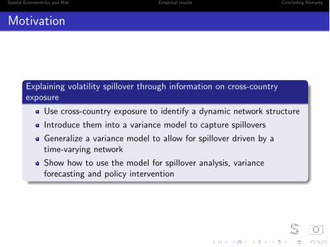
Explaining volatility spillover through information on cross-countryexposure
Use cross-country exposure to identify a dynamic network structure
Introduce them into a variance model to capture spillovers
Generalize a variance model to allow for spillover driven by atime-varying network
Show how to use the model for spillover analysis, varianceforecasting and policy intervention

Spatial Econometrics and Risk Empirical results Concluding Remarks
Spatial proximity and financial closeness
In Spatial Econometrics subjects of the analysis are neighbors in aphysical sense, and distance between subjects is measured by meansof geographical distance
From a financial viewpoint a neighboring relation (closeness,proximity) is a more elusive concept
... that cannot be translated into a physical measure(Fernadez-Aviles et al., 2012)
Possible solutions
subjects (companies) being in the same economic sector (Caporinand Paruolo, 2015)causality relations (Billio et al., 2015)cross-country exposure (this study)
Spatial Econometrics and Risk Empirical results Concluding Remarks
Financial proximity and networks
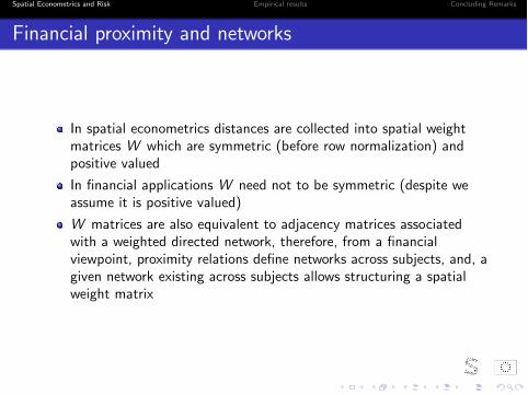
In spatial econometrics distances are collected into spatial weightmatrices W which are symmetric (before row normalization) andpositive valued
In financial applications W need not to be symmetric (despite weassume it is positive valued)
W matrices are also equivalent to adjacency matrices associatedwith a weighted directed network, therefore, from a financialviewpoint, proximity relations define networks across subjects, and, agiven network existing across subjects allows structuring a spatialweight matrix
Spatial Econometrics and Risk Empirical results Concluding Remarks
Proximity matrices for model construction
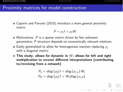
Caporin and Paruolo (2015) introduce a more general proximitymatrix
P = ⇢1I + ⇢2W
Motivations: P is a sparse matrix driven by few unknownparameters; P structure depends on economically relevant relations
Easily generalized to allow for heterogenous reaction replacing ⇢jwith a diagonal matrix
This study: allows for dynamic in W ; allows for left and right
multiplication to recover di↵erent interpretations (contributing
to/receiving from a network)
PL = diag (⇢0) I + diag (⇢1,L)Wt
PR = diag (⇢0) I +Wtdiag (⇢1,R)

Spatial Econometrics and Risk Empirical results Concluding Remarks
Proximity matrices for covariance models
Covariance models (GARCH/DCC-type, Stochastic Volatility,Realized Covariance/Correlation) su↵er for the curse ofdimensionality challenging their use with large cross-sectionaldimension for spillover analyses
Intuition: use proximity matrices to structure the model parametersand make parameters number linear in the cross-sectional dimension
Intuition: dynamic proximity matrices induce dynamic in theparameters at limited cost (they are assumed to be known)
We focus on BEKK-type specifications as we focus on covariancedynamic and for the availability of asymptotic theory
Spatial Econometrics and Risk Empirical results Concluding Remarks
BEKK and the curse of dimensionality
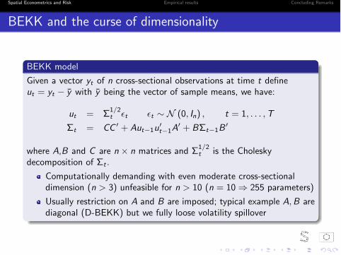
BEKK model
Given a vector yt of n cross-sectional observations at time t defineut = yt � y with y being the vector of sample means, we have:
ut = ⌃1/2t ✏t ✏t ⇠ N (0, In) , t = 1, . . . ,T
⌃t = CC
0 + Aut�1u0t�1A
0 + B⌃t�1B0
where A,B and C are n ⇥ n matrices and ⌃1/2t is the Cholesky
decomposition of ⌃t .
Computationally demanding with even moderate cross-sectionaldimension (n > 3) unfeasible for n > 10 (n = 10 ) 255 parameters)
Usually restriction on A and B are imposed; typical example A,B arediagonal (D-BEKK) but we fully loose volatility spillover
Spatial Econometrics and Risk Empirical results Concluding Remarks
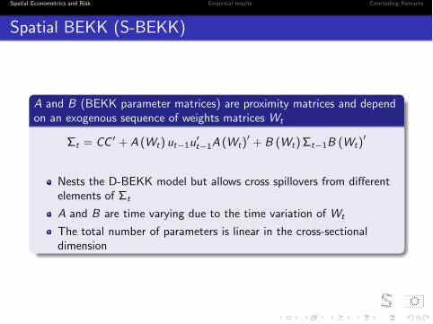
Spatial BEKK (S-BEKK)
A and B (BEKK parameter matrices) are proximity matrices and dependon an exogenous sequence of weights matrices Wt
⌃t = CC
0 + A (Wt) ut�1u0t�1A (Wt)
0 + B (Wt)⌃t�1B (Wt)0
Nests the D-BEKK model but allows cross spillovers from di↵erentelements of ⌃t
A and B are time varying due to the time variation of Wt
The total number of parameters is linear in the cross-sectionaldimension
Spatial Econometrics and Risk Empirical results Concluding Remarks
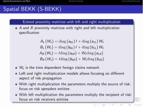
Spatial BEKK (S-BEKK)
Extend proximity matrices with left and right multiplication
A and B proximity matrices with right and left multiplicationspecification
AL (Wt) = diag (a0L) I + diag (a1L)Wt
BL (Wt) = diag (b0L) I + diag (b1L)Wt
AR (Wt) = Idiag (a0R) +Wtdiag (a1R)
BR (Wt) = Idiag (b0R) +Wtdiag (b1R)
Wt is the time dependent foreign claims network
Left and right multiplication models allows focusing on di↵erentaspect of risk propagation
With right multiplication the parameters multiply the source of risk:focus on risk spreaders entities
With left multiplication the parameters multiply the recipient of risk:focus on risk receivers entities
Spatial Econometrics and Risk Empirical results Concluding Remarks
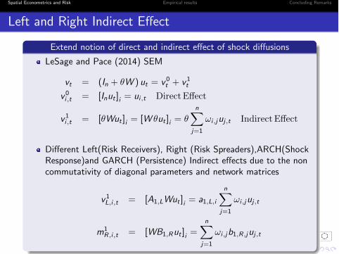
Left and Right Indirect E↵ect
Extend notion of direct and indirect e↵ect of shock di↵usions
LeSage and Pace (2014) SEM
vt = (In + ✓W ) ut = v
0t + v
1t
v
0i,t = [Inut ]i = ui,t Direct E↵ect
v
1i,t = [✓Wut ]i = [W ✓ut ]i = ✓
nX
j=1
!i,juj,t Indirect E↵ect
Di↵erent Left(Risk Receivers), Right (Risk Spreaders),ARCH(ShockResponse)and GARCH (Persistence) Indirect e↵ects due to the noncommutativity of diagonal parameters and network matrices
v
1L,i,t = [A1,LWut ]i = a1,L,i
nX
j=1
!i,juj,t
m
1R,i,t = [WB1,Rut ]i =
nX
j=1
!i,jb1,R,juj,t
Spatial Econometrics and Risk Empirical results Concluding Remarks
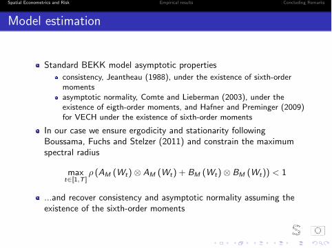
Model estimation
Standard BEKK model asymptotic properties
consistency, Jeantheau (1988), under the existence of sixth-ordermomentsasymptotic normality, Comte and Lieberman (2003), under theexistence of eigth-order moments, and Hafner and Preminger (2009)for VECH under the existence of sixth-order moments
In our case we ensure ergodicity and stationarity followingBoussama, Fuchs and Stelzer (2011) and constrain the maximumspectral radius
maxt2[1,T ]
⇢ (AM (Wt)⌦ AM (Wt) + BM (Wt)⌦ BM (Wt)) < 1
...and recover consistency and asymptotic normality assuming theexistence of the sixth-order moments
Spatial Econometrics and Risk Empirical results Concluding Remarks
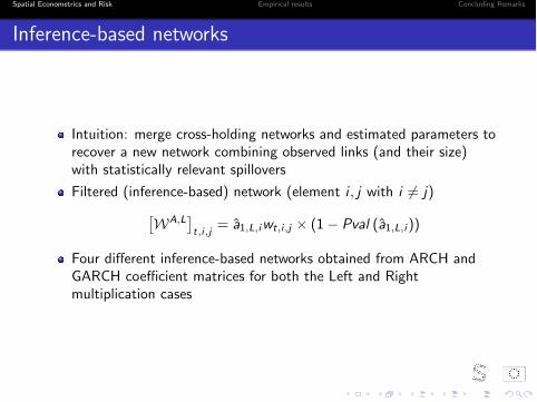
Inference-based networks
Intuition: merge cross-holding networks and estimated parameters torecover a new network combining observed links (and their size)with statistically relevant spillovers
Filtered (inference-based) network (element i , j with i 6= j)
⇥WA,L
⇤t,i,j
= a1,L,iwt,i,j ⇥ (1� Pval (a1,L,i ))
Four di↵erent inference-based networks obtained from ARCH andGARCH coe�cient matrices for both the Left and Rightmultiplication cases
Spatial Econometrics and Risk Empirical results Concluding Remarks
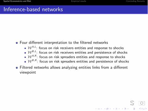
Inference-based networks
Four di↵erent interpretation to the filtered networks
WA,L: focus on risk receivers entities and response to shocksWB,L: focus on risk receivers entities and persistence of shocksWA,R : focus on risk spreaders entities and response to shocksWB,R : focus on risk spreaders entities and persistence of shocks
Filtered networks allows analyzing entities links from a di↵erentviewpoint
Spatial Econometrics and Risk Empirical results Concluding Remarks
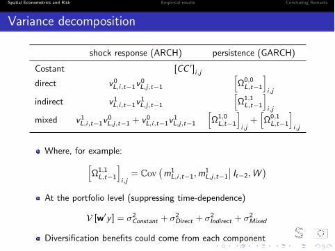
Variance decomposition
shock response (ARCH) persistence (GARCH)
Costant [CC 0]i,j
direct v
0L,i,t�1v
0L,j,t�1
h⌦0,0
L,t�1
i
i,j
indirect v
1L,i,t�1v
1L,j,t�1
h⌦1,1
L,t�1
i
i,j
mixed v
1L,i,t�1v
0L,j,t�1 + v
0L,i,t�1v
1L,j,t�1
h⌦1,0
L,t�1
i
i,j+
h⌦0,1
L,t�1
i
i,j
Where, for example:
h⌦1,1
L,t�1
i
i,j= Cov
�m
1L,i,t�1,m
1L,j,t�1
��It�2,W
�
At the portfolio level (suppressing time-dependence)
V [w0y ] = �2
Constant + �2Direct + �2
Indirect + �2Mixed
Diversification benefits could come from each component

Spatial Econometrics and Risk Empirical results Concluding Remarks
Multistep Forecast for Optimal Networks
What is the optimal network that minimizes the system conditionalvariance? What are the (target) exposures that minimize the risk inthe system?In the following we propose a forecast based criteriaTo compute multi-step-ahead forecasts we resort to a simulationapproachFirst we computed filtered innovations (standardized residuals) as
✏t = ⌃12t ut
Generate NB stationary bootstrap h�step samples from ✏Bt and thengenerate NB simulated values for ⌃t
u
Bt = ⌃
� 12
t ✏Bt⌃B
t = CC
0 + Au
B0t�1u
Bt�1A
0 + B⌃Bt�1B
0
We take as forecast the average, but even quantiles could beconsidered if we want to focus on low/high volatility level forecasts
⌃Ft =
1
NB
NBX
B=1
⌃Bt
Spatial Econometrics and Risk Empirical results Concluding Remarks
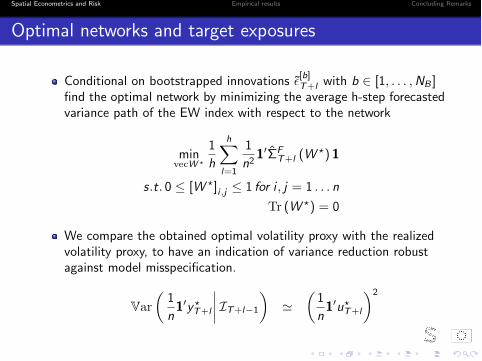
Optimal networks and target exposures
Conditional on bootstrapped innovations ✏[b]T+l with b 2 [1, . . . ,NB ]find the optimal network by minimizing the average h-step forecastedvariance path of the EW index with respect to the network
minvecW ?
1
h
hX
l=1
1
n
21
0⌃FT+l (W
?) 1
s.t. 0 [W ?]i,j 1 for i , j = 1 . . . n
Tr (W ?) = 0
We compare the obtained optimal volatility proxy with the realizedvolatility proxy, to have an indication of variance reduction robustagainst model misspecification.
Var✓1
n
1
0y
?T+l
���� IT+l�1
◆'
✓1
n
1
0u
?T+l
◆2
Spatial Econometrics and Risk Empirical results Concluding Remarks
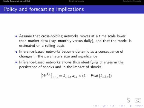
Policy and forecasting implications
Assume that cross-holding networks moves at a time scale lowerthan market data (say, monthly versus daily), and that the model isestimated on a rolling basis
Inference-based networks become dynamic as a consequence ofchanges in the parameters size and significance
Inference-based networks allows thus identifying changes in thepersistence of shocks and in the impact of shocks
⇥WA,L
⇤i,j,t
= a1,L,twi,j ⇥ (1� Pval (a1,L,t))
Spatial Econometrics and Risk Empirical results Concluding Remarks
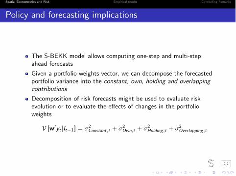
Policy and forecasting implications
The S-BEKK model allows computing one-step and multi-stepahead forecasts
Given a portfolio weights vector, we can decompose the forecastedportfolio variance into the constant, own, holding and overlapping
contributions
Decomposition of risk forecasts might be used to evaluate riskevolution or to evaluate the e↵ects of changes in the portfolioweights
V [w0yt |It�1] = �2
Constant,t + �2Own,t + �2
Holding ,t + �2Overlapping ,t
Spatial Econometrics and Risk Empirical results Concluding Remarks
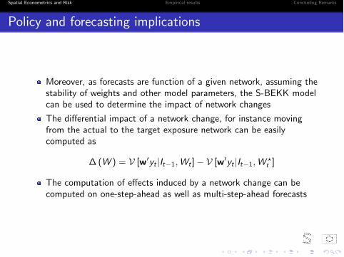
Policy and forecasting implications
Moreover, as forecasts are function of a given network, assuming thestability of weights and other model parameters, the S-BEKK modelcan be used to determine the impact of network changes
The di↵erential impact of a network change, for instance movingfrom the actual to the target exposure network can be easilycomputed as
� (W ) = V [w0yt |It�1,Wt ]� V [w0
yt |It�1,W?t ]
The computation of e↵ects induced by a network change can becomputed on one-step-ahead as well as multi-step-ahead forecasts
Spatial Econometrics and Risk Empirical results Concluding Remarks
Data description
Changes in the ten-year sovereign bond yields
Sample size January 2006 - December 2013, coherently with thecross country holding data
Model daily data with network evolving at a lower time scale,quarterly
Networks estimated from BIS data with normalization associatedwith the total amount of bank exposures (thus not restricting thenormalization to the analyzed countries)
Spatial Econometrics and Risk Empirical results Concluding Remarks
Dependence Network from Foreign Claims
Spatial Econometrics and Risk Empirical results Concluding Remarks
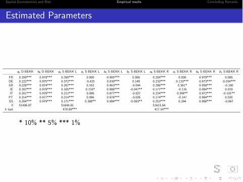
Estimated Parameters
a0 D-BEKK b0 D-BEKK a0 S-BEKK L a1 S-BEKK L b0 S-BEKK L b1 S-BEKK L a0 S-BEKK R a1 S-BEKK R b0 S-BEKK R b1 S-BEKK R
FR 0.209*** 0.978*** 0.260*** 0.000 0.965*** 0.000 0.204*** 0.000 0.979*** 0.000DE 0.222*** 0.975*** 0.372*** -0.425 0.930*** 0.149 0.232*** 0.133*** 0.973*** -0.034***GR 0.228*** 0.974*** 0.267*** 0.163 0.963*** -0.044 0.286*** 0.361* 0.958*** -0.100IE 0.202*** 0.979*** 0.165*** 0.216* 0.986*** -0.047** 0.177*** -0.116 0.984*** 0.019IT 0.201*** 0.978*** 0.212*** 0.086 0.977*** -0.027 0.224*** 0.398** 0.972*** -0.101**PT 0.214*** 0.977*** 0.214*** 0.096 0.976*** -0.026 0.174*** -0.147 0.984*** 0.020ES 0.204*** 0.979*** 0.171*** 0.388** 0.984*** -0.083** 0.253*** 0.294 0.968*** -0.067ll 51406.87 51646.81 51615.64
lr test 479.89*** 417.54***
* 10% ** 5% *** 1%
Spatial Econometrics and Risk Empirical results Concluding Remarks
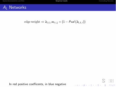
AL
Networks
edgeweight ) a1,L,iwt,i,j ⇥ (1� Pval (a1,L,i ))
In red positive coe�cents, in blue negative
Spatial Econometrics and Risk Empirical results Concluding Remarks
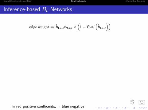
Inference-based BL
Networks
edgeweight ) b1,L,iwt,i,j ⇥⇣1� Pval
⇣b1,L,i
⌘⌘
In red positive coe�cents, in blue negative
Spatial Econometrics and Risk Empirical results Concluding Remarks
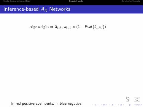
Inference-based AR
Networks
edgeweight ) a1,R,iwt,i,j ⇥ (1� Pval (a1,R,i ))
In red positive coe�cents, in blue negative
Spatial Econometrics and Risk Empirical results Concluding Remarks
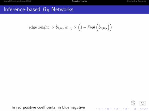
Inference-based BR
Networks
edgeweight ) b1,R,iwt,i,j ⇥⇣1� Pval
⇣b1,R,i
⌘⌘
In red positive coe�cents, in blue negative
Spatial Econometrics and Risk Empirical results Concluding Remarks
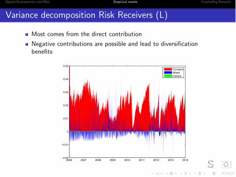
Variance decomposition Risk Receivers (L)
Most comes from the direct contribution
Negative contributions are possible and lead to diversificationbenefits
2006 2007 2008 2009 2010 2011 2012 2013 2014−0.02
−0.01
0
0.01
0.02
0.03
0.04
0.05
ConstantMixedIndirect
Spatial Econometrics and Risk Empirical results Concluding Remarks
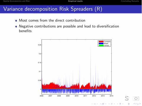
Variance decomposition Risk Spreaders (R)
Most comes from the direct contribution
Negative contributions are possible and lead to diversificationbenefits
2006 2007 2008 2009 2010 2011 2012 2013 2014
0
0.05
0.1
0.15
0.2
0.25
ConstantMixedIndirect
Spatial Econometrics and Risk Empirical results Concluding Remarks
Optimal networks
Forecast one quarter ahead for quarter II of 2010
Recover the optimal target network exposure for both risk receiversand risk spreaders
Constrained optimization implies a redistribution of the claimsamong the considered countries
Unconstrained optimization means that the total amount of claimschanges for each country
Spatial Econometrics and Risk Empirical results Concluding Remarks
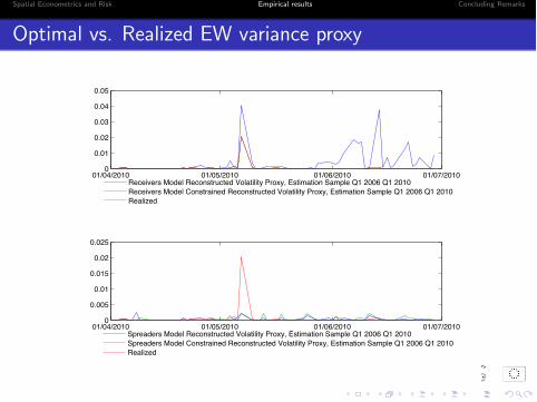
Optimal vs. Realized EW variance proxy
01/04/2010 01/05/2010 01/06/2010 01/07/20100
0.01
0.02
0.03
0.04
0.05
Receivers Model Reconstructed Volatility Proxy, Estimation Sample Q1 2006 Q1 2010Receivers Model Constrained Reconstructed Volatility Proxy, Estimation Sample Q1 2006 Q1 2010Realized
01/04/2010 01/05/2010 01/06/2010 01/07/20100
0.005
0.01
0.015
0.02
0.025
Spreaders Model Reconstructed Volatility Proxy, Estimation Sample Q1 2006 Q1 2010Spreaders Model Constrained Reconstructed Volatility Proxy, Estimation Sample Q1 2006 Q1 2010Realized
Spatial Econometrics and Risk Empirical results Concluding Remarks
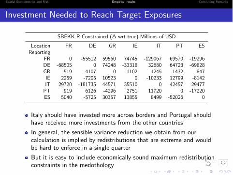
Investment Needed to Reach Target Exposures
SBEKK R Constrained (� wrt true) Millions of USD
Location FR DE GR IE IT PT ESReporting
FR 0 -55512 59560 74745 -129067 69570 -19296DE -68505 0 74248 -33318 32680 64723 -69828GR -519 -4107 0 1102 1245 1432 847IE 2259 -7205 10523 0 -10233 12799 -8142IT 29720 -181735 44571 35510 0 42457 29477PT 919 6126 -4296 2751 11720 0 -17220ES 5040 -5725 30357 13855 8499 -52026 0
Italy should have invested more across borders and Portugal shouldhave received more investments from the other countries
In general, the sensible variance reduction we obtain from ourcalculation is implied by redistributions that are extreme and wouldbe hard to enforce in a single quarter
But it is easy to include economically sound maximum redistributionconstraints in the medothology

Spatial Econometrics and Risk Empirical results Concluding Remarks
Concluding remarks
Concluding remarks
In the European sovereign bond markets part of spillover e↵ects canbe traced back to a physical claim channel: banks’ foreign exposures
Germany, Italy and, to a lesser extent, Greece are playing a centralrole in spreading risk
Ireland and Spain are the most susceptible receivers of spillovere↵ects
Acting on these physical channels before the sovereign crisis, itwould have been possible to have a clear risk mitigation outcome
In progress
Di↵erent Asset Classes (In particular equity )
Inclusion of more countries
Joint Left and Right multiplication model
introduce in the model more networks, jointly, to test and comparethem

Spatial Econometrics and Risk Empirical results Concluding Remarks
Thank You!


![MGARCH[0.7cm] An R Package for Fitting Multivariate GARCH ... · An R Package for Fitting Multivariate GARCH Models ... Schmidbauer / V.S. Tunal o glu ... o glu / A. R oschOPEC News](https://img.pdfslide.us/doc/110x75/5bb578cf09d3f2e1768cee83/mgarch07cm-an-r-package-for-fitting-multivariate-garch-an-r-package-for.jpg)