Embed Size (px)
Citation preview
Military Buildups&
Economic Growth
Kenwin Maung
Agenda
1. Review of Ramey and Shapiro (1998)
2. My ARDL Model Specification
3. Inference and Comparison
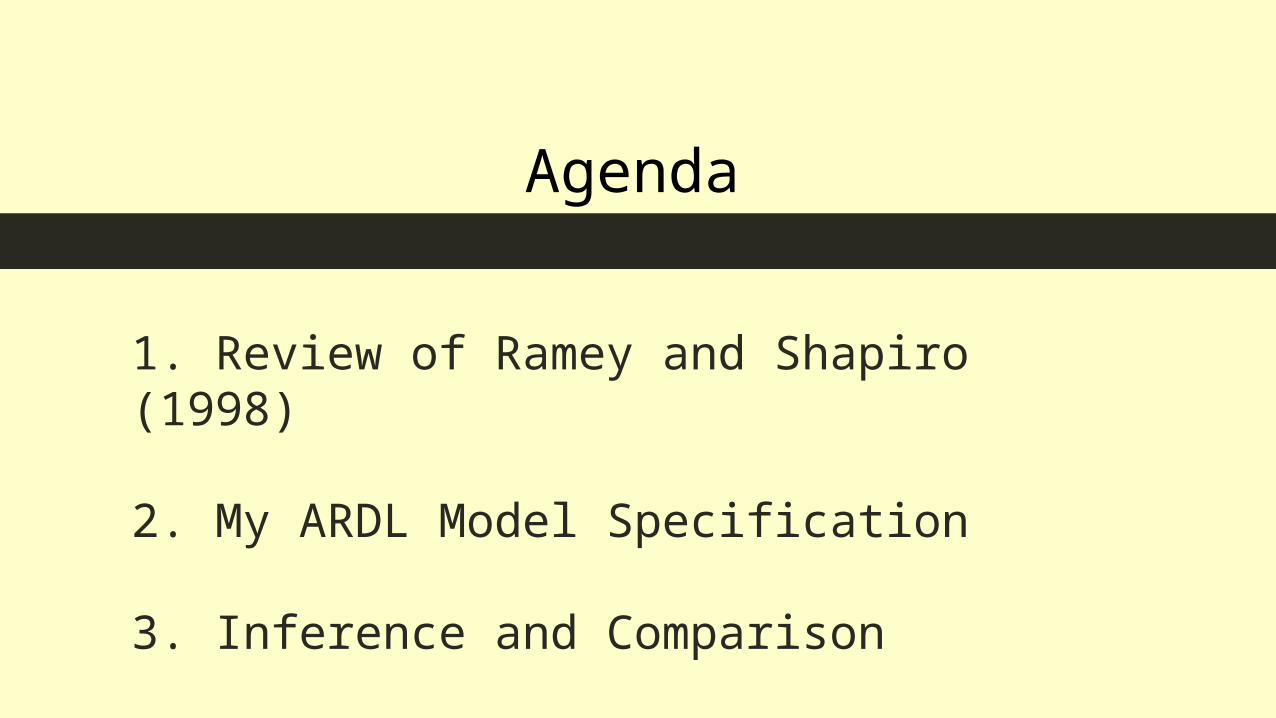
Costly capital reallocation and the effects of government spending (1998)
𝒚 𝒕=𝜶𝟎+𝜶𝟏𝒕+𝜶𝟐(𝒕≥𝟏𝟗𝟕𝟑 :𝟐)+∑𝒊=𝟏
𝟖𝒃𝒊 𝒚 𝒕−𝟏+∑
𝒊=𝟎
𝟖𝒄𝒊𝑫𝒕−𝒊+𝝐𝒕
Where: is the endogenous variable is a time trend starting from 1947:1 and is a time trend starting from 1973:2 is the buildup dummy taking1 for 1950:3, 1965:1, and 1980:1
Sample period 1947:1 to 1996:4
Review of Ramey & Shapiro
Costly capital reallocation and the effects of government spending (1998)
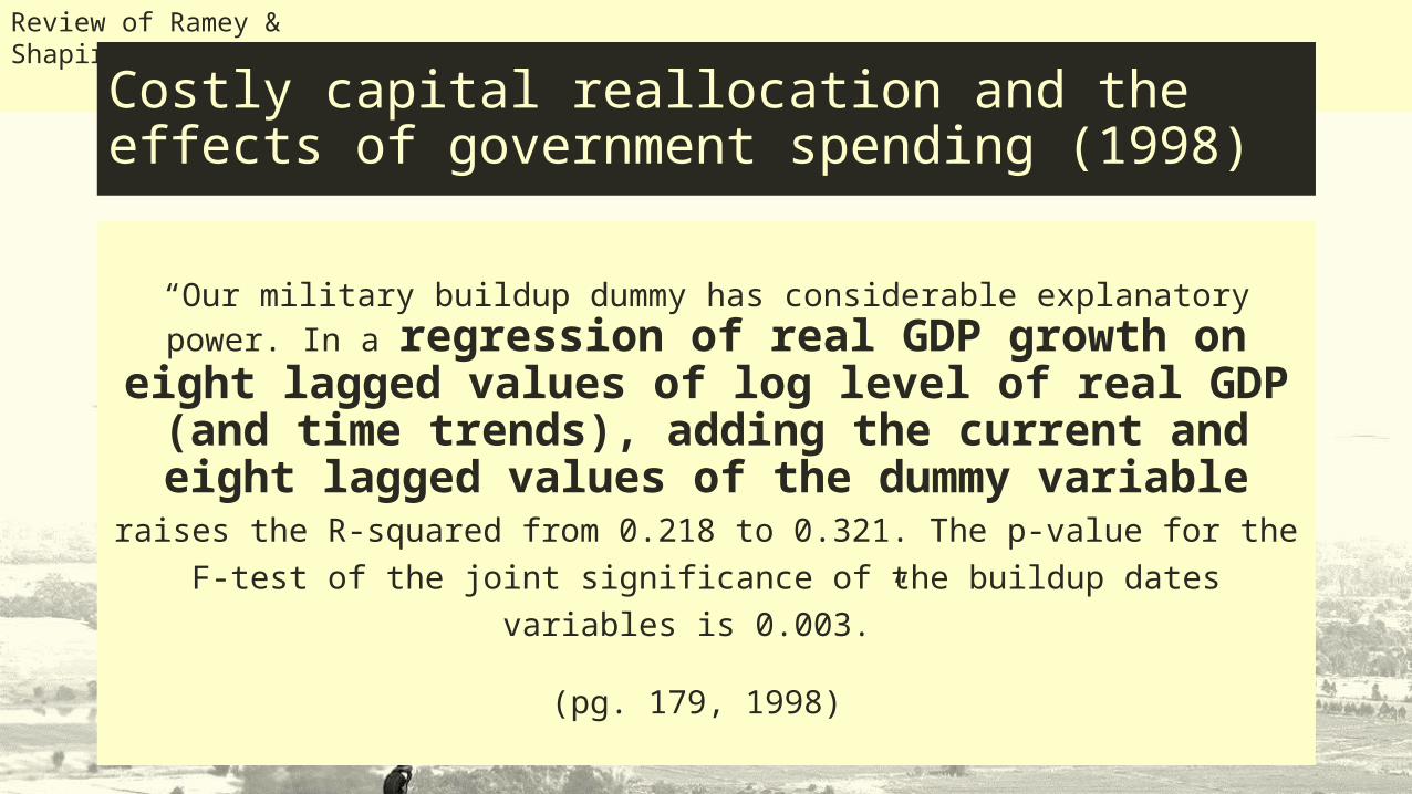
“Our military buildup dummy has considerable explanatory power. In a regression of real GDP growth on eight lagged
values of log level of real GDP (and time trends), adding the current and eight lagged
values of the dummy variable raises the R-squared from 0.218 to 0.321. The p-value for the F-test of the joint significance of the
buildup dates variables is 0.003.”
(pg. 179, 1998)
Review of Ramey & Shapiro
Costly capital reallocation and the effects of government spending (1998)
Review of Ramey & Shapiro
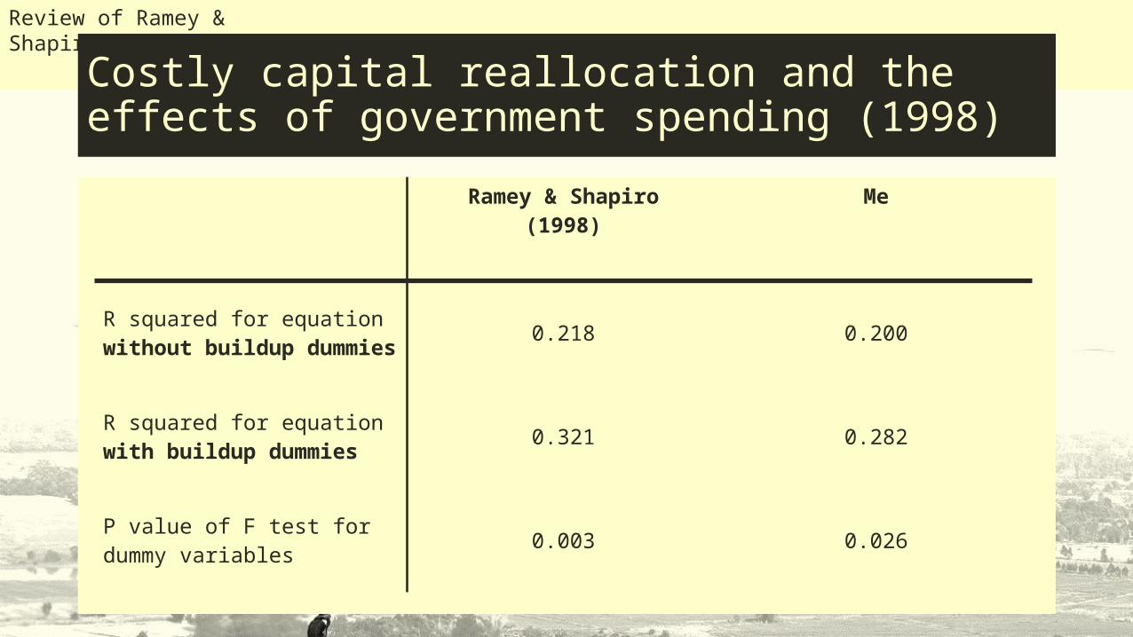
Ramey & Shapiro(1998)
Me
R squared for equation without buildup dummies
0.218 0.200
R squared for equation with buildup dummies 0.321 0.282
P value of F test for dummy variables 0.003 0.026
My model specification
Data definitions
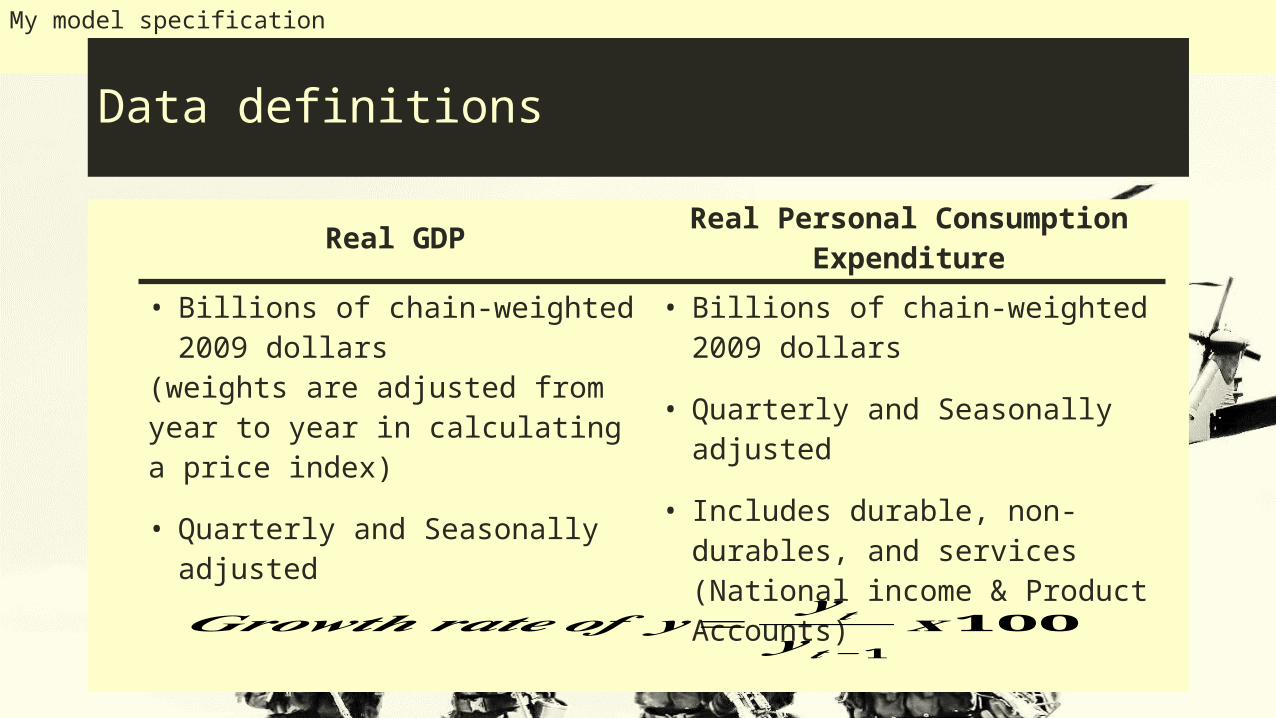
Real GDP Real Personal Consumption Expenditure
• Billions of chain-weighted 2009 dollars
(weights are adjusted from year to year in calculating a price index)• Quarterly and Seasonally
adjusted
• Billions of chain-weighted 2009 dollars
• Quarterly and Seasonally adjusted
• Includes durable, non-durables, and services (National income & Product Accounts)
𝑮𝒓𝒐𝒘𝒕𝒉𝒓𝒂𝒕𝒆𝒐𝒇 𝒚=𝒚 𝒕
𝒚 𝒕−𝟏𝐱𝟏𝟎𝟎
My model specification
Tweaking the model
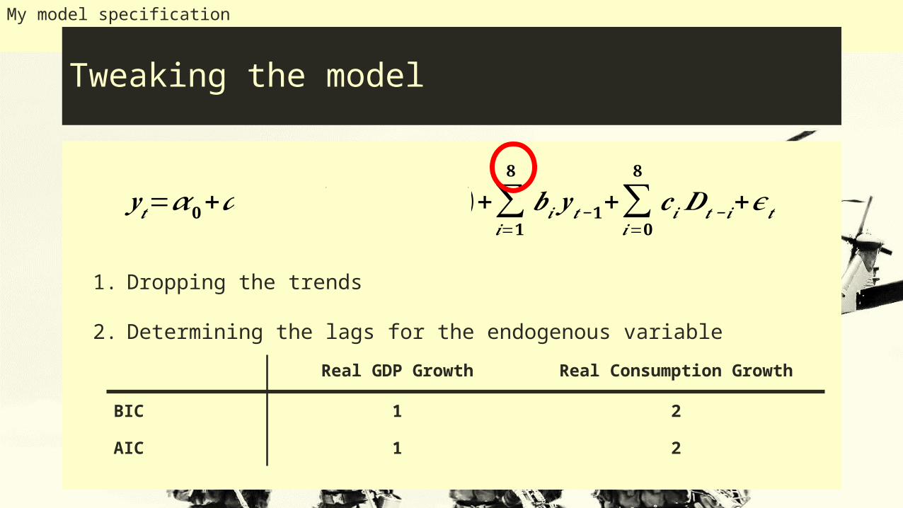
𝒚 𝒕=𝜶𝟎+𝜶𝟏𝒕+𝜶𝟐(𝒕≥𝟏𝟗𝟕𝟑 :𝟐)+∑𝒊=𝟏
𝟖𝒃𝒊 𝒚 𝒕−𝟏+∑
𝒊=𝟎
𝟖𝒄𝒊𝑫𝒕−𝒊+𝝐𝒕
1. Dropping the trends
2. Determining the lags for the endogenous variableReal GDP Growth Real Consumption Growth
BIC 1 2
AIC 1 2
My model specification
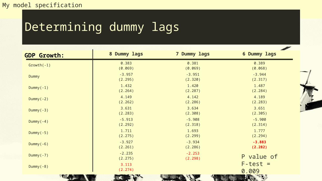
Determining dummy lags
GDP Growth: 8 Dummy lags 7 Dummy lags 6 Dummy lags
Growth(-1) 0.383(0.069)
0.381(0.069)
0.389(0.068)
Dummy -3.957(2.295)
-3.951(2.320)
-3.944(2.317)
Dummy(-1) 1.432(2.264)
1.420(2.287)
1.487(2.284)
Dummy(-2) 4.149(2.262)
4.142(2.286)
4.189(2.283)
Dummy(-3) 3.631(2.283)
3.634(2.308)
3.651(2.305)
Dummy(-4) -5.913(2.292)
-5.908(2.318)
-5.900(2.314)
Dummy(-5) 1.711(2.275)
1.693(2.299)
1.777(2.294)
Dummy(-6) -3.927(2.261)
-3.934(2.286)
-3.883(2.282)
Dummy(-7) -2.235(2.275)
-2.253(2.298)
Dummy(-8) 3.113(2.274)
P value of F-test = 0.009
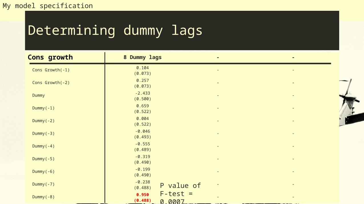
My model specification
Determining dummy lagsCons growth 8 Dummy lags - -
Cons Growth(-1) 0.104(0.073) - -
Cons Growth(-2) 0.257(0.073) - -
Dummy -2.433(0.500) - -
Dummy(-1) 0.659(0.522) - -
Dummy(-2) 0.004(0.522) - -
Dummy(-3) -0.046(0.493) - -
Dummy(-4) -0.555(0.489) - -
Dummy(-5) -0.319(0.490) - -
Dummy(-6) -0.199(0.490) - -
Dummy(-7) -0.238(0.488) - -
Dummy(-8) 0.950(0.488) - -
P value of F-test = 0.0007
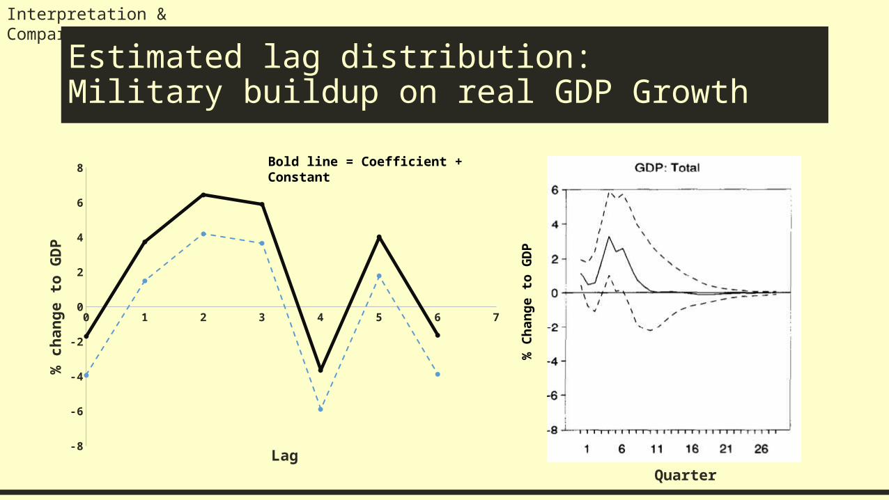
Interpretation & Comparison
Estimated lag distribution:Military buildup on real GDP Growth
0 1 2 3 4 5 6 7
-8
-6
-4
-2
0
2
4
6
8
Lag
% c
hang
e to
GDP
Quarter
Bold line = Coefficient + Constant
% C
hang
e to
GD
P
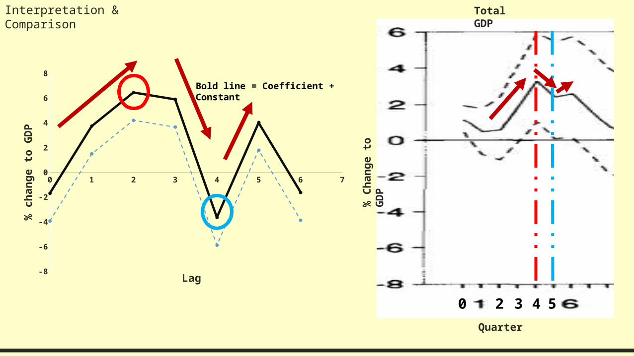
Interpretation & Comparison
Quarter
0 1 2 3 4 5 6 7
-8
-6
-4
-2
0
2
4
6
8
Lag
% c
hang
e to
GDP
Total GDP
% C
hang
e to
G
DP
Bold line = Coefficient + Constant
0 2 3 4 5
0 1 2 3 4 5 6 7 8 9
-3-2.5
-2-1.5
-1-0.5
00.5
11.5
2
Lag
% C
hang
e to
Con
-su
mpt
ion
Interpretation & Comparison
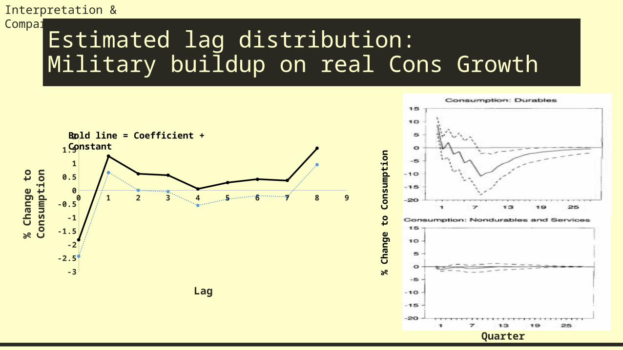
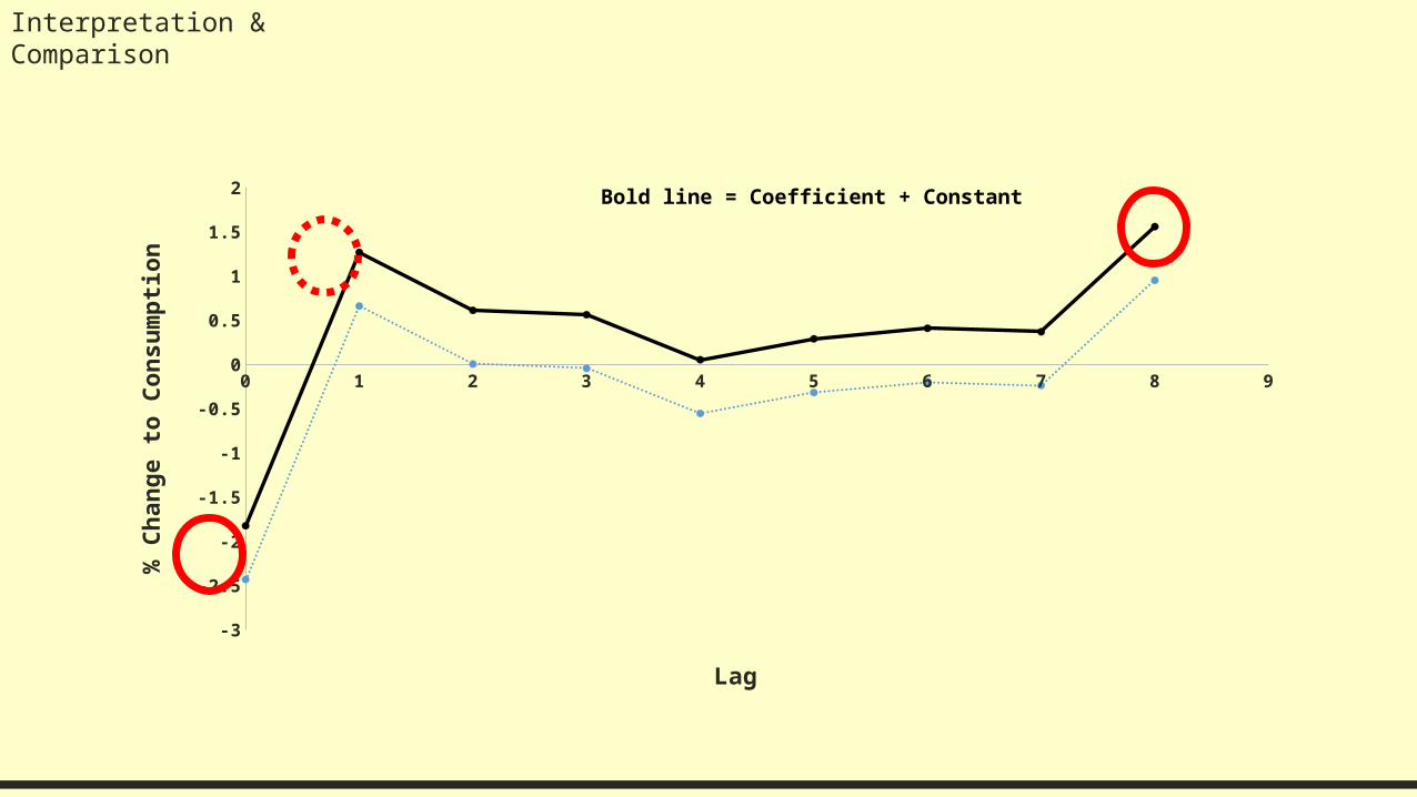
Estimated lag distribution:Military buildup on real Cons Growth
Quarter
Bold line = Coefficient + Constant
% C
hang
e to
Con
sum
ptio
n
0 1 2 3 4 5 6 7 8 9
-3
-2.5
-2
-1.5
-1
-0.5
0
0.5
1
1.5
2
Lag
% C
hang
e to
Con
sum
ptio
n
Interpretation & Comparison
Bold line = Coefficient + Constant
Thank
you
Kenwin Maung
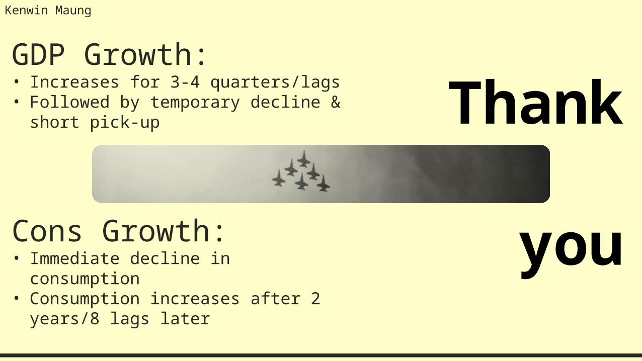
GDP Growth:• Increases for 3-4 quarters/lags• Followed by temporary decline &
short pick-up
Cons Growth:• Immediate decline in consumption• Consumption increases after 2
years/8 lags later