Forward Guidance & Heterogenous Beliefs, Andrade, Gaballo, Mengus & Mojon

Forward Guidance and Heterogenous Beliefs

Philippe Andrade(BdF)

Gaetano Gaballo(ECB & BdF)

Eric Mengus(HEC Paris)

Benoit Mojon(BdF)

International WorkshopMonetary Policy when Heterogeneity Matters

Paris – February 3, 2017

The views expressed here are the authors’ and do not necessarily representthose of the European Central Bank, Banque de France or the Eurosystem.

FG in theoryKrugman, Eggertsson-Woodford, Werning

More accommodation at the ZLB?

I Promise to keep interest rate at zero beyond the end of the trap

I engineer expectations of a boom tomorrow;

I positive impact today through real interest rate / Euler eq.;

I second best: shortens recession but transitory future inflation;

I time-inconsistent: CB prefers not to inflate at the end of the trap.

I Needs agents understand policy & trust CB’s commitment(Woodford, 2012).

FG in practiceFG statements not always clear

Ex: FOMC – Aug. 9, 2011; beginning of date-based FG (DBFG)

The Committee currently anticipates that economic conditions[...] are likely to warrant exceptionally low levels for the federalfunds rate at least through mid-2013. [...]

Two potential meanings (Campbell et al., 2012):

I “Odyssean”: commitment to future accommodation.

I “Delphic”: signal about future state.

FG in “puzzles”

I Strong impact on expected short term IR (Swansson-Williams, 2014)

I But consumption, investment, activity, inflation did not react much.

I At odd, with incredibly strong macroeconomic impact in models.

I “Forward guidance puzzle” (Del Negro, Giannoni & Patterson, 2015).

I How to explain that expectations about rates moved so much butagents reacted so little?

I The problem is the NK model: credit constraints (MsKay et al.,2014), bounded rationality (Gabaix, 2016), imperfect information(Angeletos 2016), etc...

Our approach is cross-sectional

The problem is the announcement: promise to keep rates at zero for awhile can be interpreted differently:

I people agree on the path of rates but (agree to) disagree on policy

I commitment cannot be observed, low rates anyway

I some agents revise their expectations about the state of theeconomy upwards, some other downwards

I announcements had huge cross-sectional impact and little on average

Our Contributions: facts + model + optimal policy.

Literature

I Optimal policy at ZLB: Krugman (1998), Eggertsson & Woodford(2003), Werning (2012), Bassetto (2015), Bilbiie (2016).

I FG less potent with imperfect credit markets: McKay et al. (2014),Del Negro et al. (2015).

I Potential detrimental impact of FG with heterogenous agents:Michelacci & Paciello (2016).

I Dispersed beliefs / imperfect info at the ZLB: Wiederholt (2014).

I Monetary policy conveys info on future state: Romer & Romer(2000), Gurkaynak et al. (2005), Melosi (2014).

I Disagreement informative for macro: Mankiw et al. (2003); Coibion& Gorodnichenko (2012); Andrade et al. (2013).

Data

I US SPF.

I Real consumption growth (∆c), CPI inflation (π), 3M-Tbills (r).

I Sample: 1982:Q1-2014:Q4.

I Forecast horizons: 1Q, 1Y & 2Y.

I Individual forecasts (cross-section dispersion).

I Disagreement: 75th − 25th quantiles.

Disagreement about future short-term interest ratesHistorically low starting date-based FG

2002 2004 2006 2008 2010 2012 2014 20160

0.1

0.2

0.3

0.4

0.5

0.6

0.7

0.8

0.9

1

Figure: Disagreement about future 3-month interest rates 1Q (black), 1Y (red)and 2Y (blue) ahead. (Inter-quantile range in US-SPF, 4-quarter moving average)

Disagreement about future consumption / inflationWithin historical range during FG

Consumption Inflation

2002 2004 2006 2008 2010 2012 2014 20160

0.5

1

1.5

2

2.5

2002 2004 2006 2008 2010 2012 2014 20160

0.5

1

1.5

2

2.5

Figure: Disagreement about future consumption growth and inflation 1Q(black), 1Y (red) and 2Y (blue) ahead. (Inter-quantile range in US-SPF, 4-quarter moving average)

Testing heterogeneity

Define two groups of forecasters at DBFG dates:

optimists: revision of both consumption and inflation > average

pessimists: revision of both consumption and inflation < average

1. Was the average revision of consumption (resp. inflation) byoptimists statistically different from the one of pessimists? and fromthe one of the rest of the population?

2. Do we find similar statistical difference in the revision of interestrates?

3. If we extrapolate Taylor rules from past revisions to projectimplied shadow rates from current expectations on inflation andconsumption, do we see similar statistical differences in the revisionof shadow interest rates?

4. Do we see any evidence of change in the correlation betweenrevisions of interest rate and inflation at the individual level afterDBFG?

Two groups of forecasters at date-based FG announcement

Forecast revisions Optimists Pessimists Not Optimists2011Q4Share of individuals 19% 29% 81%Consumption .32 (.28) [**,#] -.20 (.19) -.05 (.41)Inflation .19 (.22) [**/#] -.22 (.14) -.12 (.55)Nominal rates -.41 (.46) -.38 (.30) -.42 (.44)Shadow Taylor-rate .35 (.25) [***/###] -.37 (.14) -.16 (.37)2012Q1Share of individuals 22% 23% 78%Consumption .79 (.33) [***/##] .13 (.24) .19 (.24)Inflation .48 (.29) [***/###] -.26 (.29) -.12 (.30)Nominal rates -.37 (.55) -.04 (.08) -.04 (.07)Shadow Taylor-rate .86 (.55) [**/#] -.17 (.31) .05 (.35)2012Q4Share of individuals 36% 24% 64%Consumption .20 (.19) [***/###] -.26 (.22) -.21 (.26)Inflation .19 (.23) [***/#] -.32 (.32) -.17 (.36)Nominal rates -.04 (.15) .02 (.02) -.02 (.06)Shadow Taylor-rate .23 (.30) [***/##] -.36 (.27) -.27 (.26)Corr(rev. inflation, rev. rates)2009Q1-2011Q3 .41 (.07) .15 (.07) .24 (.07)2011Q4-2012Q4 -.26 (.20) .38 (.25) .22 (.15)































Excess disagreement on future infl. / cons.Starting date-based FG

I Estimate link btw disagreements pre-crisis

DIS(xh) = α + βDIS(ih) + γDIS(x1q) + ε

ε (x =INF, h = 2y) ε (x =CONS, h = 2y)

2002 2004 2006 2008 2010 2012 2014 2016-0.5

0

0.5

1

Further evidenceComparable evidence in HHs survey (Michigan)

I The share of HHs expecting constant / decreasing IR over next 12Mreached a historical high >70%

I Optimists: better business condition & inflation above averagePessimists: worse business conditions & inflation below average

Optimists Pessimists Not OptimistsAverages observed in 2011m9

Fraction of respondents 5% 50% 95%Good times for durable .50 .27 .25Inflation 6.64 1.77 3.51

Averages observed in 2012m2Fraction of respondents 13% 28% 87%Good times for durable .55 .30 .36Inflation 5.50 1.37 3.10

Averages observed in 2012m10Fraction of respondents 15% 30% 85%Good times for durable .46 .24 .29Inflation 7.34 1.95 3.37

Table: Average of qualitative forecasts across groups of households.

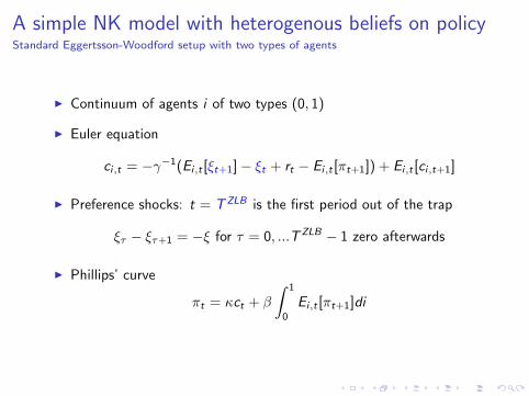
A simple NK model with heterogenous beliefs on policyStandard Eggertsson-Woodford setup with two types of agents

I Continuum of agents i of two types (0, 1)

I Euler equation

ci,t = −γ−1(Ei,t [ξt+1]− ξt + rt − Ei,t [πt+1]) + Ei,t [ci,t+1]

I Preference shocks: t = TZLB is the first period out of the trap

ξτ − ξτ+1 = −ξ for τ = 0, ...TZLB − 1 zero afterwards

I Phillips’ curve

πt = κct + β

∫ 1

0

Ei,t [πt+1]di

A simple NK model with heterogenous beliefs on policyIntuition

I Shocks to the discount factor ⇒ ZLB for TZLB periods.

I Agents agree on TCB periods of rates at ZLB (then back to normal).

I Private sector does not observe TZLB and disagrees on CB’s type:

1 − α believe CB is of Odyssean type: E0,opt [TZLB ] < TCB

α believe CB is of Delphic type: E0,pess [TZLB ] = TCB

I Agreement on TCB but disagreement on periods of extraaccommodation TCB − TZLB .

A simple NK model with heterogenous beliefs on policyEquilibrium

For a given sequence of shocks ξ0, ξ1, ..., we focus on an equilibrium attime t = 0 that satisfies:

I agents optimize given homogeneous beliefs about the length of thetrap

I agents believe the central bank set rates optimally, but does notobserve commitment ability

I beliefs (length of the trap; commitment) are consistent with thecurrent allocation

I markets clear

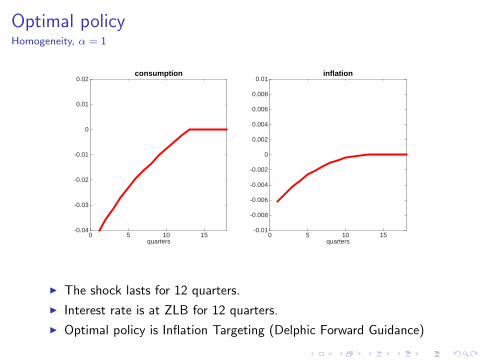
Optimal policyHomogeneity, α = 1

quarters0 5 10 15

-0.04

-0.03

-0.02

-0.01

0

0.01

0.02consumption

quarters0 5 10 15

-0.01

-0.008

-0.006

-0.004

-0.002

0

0.002

0.004

0.006

0.008

0.01inflation

I The shock lasts for 12 quarters.

I Interest rate is at ZLB for 12 quarters.

I Optimal policy is Inflation Targeting (Delphic Forward Guidance)

Optimal policyHomogeneity, α = 0

quarters0 5 10 15

-0.04

-0.03

-0.02

-0.01

0

0.01

0.02consumption

quarters0 5 10 15

-0.01

-0.008

-0.006

-0.004

-0.002

0

0.002

0.004

0.006

0.008

0.01inflation


I Interest rate is at ZLB for 12+5 quarters.

I Optimal policy is Odyssean FG

Optimal policyHeterogeneity α = 0.1

quarters0 5 10 15

-0.04

-0.03

-0.02

-0.01

0

0.01

0.02consumption

quarters0 5 10 15

-0.01

-0.008

-0.006

-0.004

-0.002

0

0.002

0.004

0.006

0.008

0.01inflation



I More aggressive Odyssean FG is optimal (Bodenstein et al., 2012)

How the model works: actionsHeterogeneity α = 0.1

quarters0 5 10 15

-0.04

-0.03

-0.02

-0.01

0

0.01

0.02consumption

act. aggr. optFG act. aggr. Taylor act. ind. opt. act. ind. pess.

quarters0 5 10 15

-0.01

-0.008

-0.006

-0.004

-0.002

0

0.002

0.004

0.006

0.008

0.01inflation



I Aggregate consumption lower / optimists (FG puzzle).

How the model works: expectations at time 0Heterogeneity α = 0.1

quarters0 5 10 15

-0.04

-0.03

-0.02

-0.01

0

0.01

0.02consumption

act. aggr. optFG act. aggr. Taylor exp. opt. exp. pess.

quarters0 5 10 15

-0.01

-0.008

-0.006

-0.004

-0.002

0

0.002

0.004

0.006

0.008

0.01inflation

act. optFG act. Taylor exp. opt. exp. pess.


I Agents agree on interest rate at ZLB for 12+6 quarters.

I Agents disagree on inflation and consumption at the end of the trap.

Optimal policyVarying heterogeneity: α = 0.3

quarters0 5 10 15

-0.04

-0.03

-0.02

-0.01

0

0.01

0.02consumption

quarters0 5 10 15

-0.01

-0.008

-0.006

-0.004

-0.002

0

0.002

0.004

0.006

0.008

0.01inflation



Agents disagree on inflation and consumption at the end of the trap.

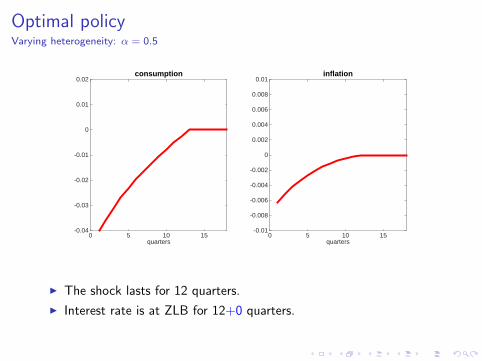
Optimal policyVarying heterogeneity: α = 0.5

quarters0 5 10 15

-0.04

-0.03

-0.02

-0.01

0

0.01

0.02consumption

quarters0 5 10 15

-0.01

-0.008

-0.006

-0.004

-0.002

0

0.002

0.004

0.006

0.008

0.01inflation



Agents disagree on inflation and consumption at the end of the trap.

Optimal Policy with Disagreement

fraction of pessimists α0 0.1 0.2 0.3 0.4 0.5 0.6 0.7 0.8 0.9 1

FG

extr

a p

erio

ds o

f a

cco

mo

da

tio

n

TC

B-

T

0

1

2

3

4

5

6

7

8

9

10

11

12

13

14

15

16

low shock

high shock

I Trade-off: further accommodation makes delphic more pessimistic.

Conclusion

1. Evidence specific to DBFG period:

I Agents agreed on interest rate / disagreed on macro var.

I Two interpretations of same policy coexisted.

2. We build a std NK model with heterogenous beliefs where:

I Agents agree on interest rate but disagree on policy;

I FG is less effective than pure odyssean FG;

I Odyssean FG is not always optimal.

3. Policy implications:

I Underline limits of looking at (expected) int. rates to assess FGeffectiveness.

I Emphasize credibility of CB’s commitment is key when conductingFG (communication? QE?).

Appendix

FG very effective on IR

2008 2009 2010 2011 2012 2013 2014 20150

0.5

1

1.5

2

2.5

3

3.5

Figure: Expected federal fund rates 1Q (black), 1.5Y (red) and 2Y (blue)ahead. (from OIS, 5-day average after FOMC dates)

Can agents agree on future rates but disagree onfundamentals?Intuition

I Yes: agree on futures rates but disagree on policy

I Simple policy rule:r = φΩ + δ.

I Future interest rate expected by individual i :

E it (r) = φE i

t (Ω) + E it (δ).

I Heterogeneity in deviations E it (δ) offsets heterogeneity in

fundamentals E it (Ω) .

I Optimistic on fundamentals E jt (Ω) > 0 sees accommodative

deviations E jt (δ) < 0.

I Pessimistic on fundamentals E it (Ω) < 0 sees restrictive deviations

E it (δ) > 0.

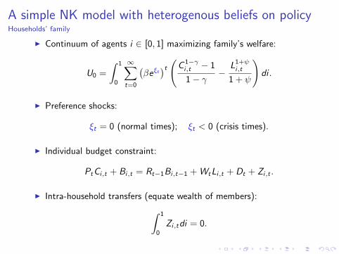
A simple NK model with heterogenous beliefs on policyHouseholds’ family

I Continuum of agents i ∈ [0, 1] maximizing family’s welfare:

U0 =

∫ 1

0

∞∑t=0

(βeξt

)t (C 1−γi,t − 1

1− γ−

L1+ψi,t

1 + ψ

)di .

I Preference shocks:

ξt = 0 (normal times); ξt < 0 (crisis times).

I Individual budget constraint:

PtCi,t + Bi,t = Rt−1Bi,t−1 + WtLi,t + Dt + Zi,t .

I Intra-household transfers (equate wealth of members):∫ 1

0

Zi,tdi = 0.

A simple NK model with heterogenous beliefs on policyFirms

I Final good production:

Yt =

(∫Y

θ−1θ

j,t dj

) θθ−1

.

I Intermediate goods production:

Yj,t = Lj,t .

I Intermediate goods producers subject to Calvo pricing (proba 1−χ).

A Simple NK Model with Heterogenous BeliefsEquilibrium

For a given sequence of shocks ξ0, ξ1, ..., an equilibrium at time t = 0is defined by the following conditions:

i) given a sequence of policy deviations ∆0,∆1, ... and a set ofbeliefs [pes, opt] about the end of the trap / the type of the CB,

Ci,t , Li,t ,Bi,t ,Dt ,Rt ,Wt ,Zi,t ,Pti∈[pes,opt],t≥0

solve household’s and firms’ problems, satisfy the monetary policyrule and clear markets;

ii) given agents’ beliefs and optimal actions, ∆0,∆1, ... minimizesCB’s loss function;

iii) agents beliefs (trap, commitment) are updated following Bayes’ law(and consistent with current allocations).

Inflation Targeting (Delphic Forward Guidance)

time Ei,0 [ci,t ], α = 1

t > TCB 0

t = TCB γ−1(logR)

T < t< TCB 0

t = T γ−1(logR − ξ)+Ei,0 [πt+1]) + Ei,0 [ci,t+1]

0 < t < T γ−1(logR − ξ) + Ei,0 [πt+1]) + Ei,0 [ci,t+1]

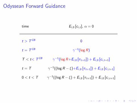
Odyssean Forward Guidance

time Ei,0 [ci,t ], α = 0

t > TCB 0

t = TCB γ−1(logR)

T < t< TCB γ−1(logR+Ei,0 [πt+1]) + Ei,0 [ci,t+1]

t = T γ−1((logR − ξ)+Ei,0 [πt+1]) + Ei,0 [ci,t+1]

0 < t < T γ−1((logR − ξ) + Ei,0 [πt+1]) + Ei,0 [ci,t+1]

How FG was communicated?Fed experience: weak coordination of opinions

Federal Reserve press release of January 28, 2009:

The Federal Open Market Committee decided today to keep itstarget range for the federal fund rate at 0 to 1/4 percent. TheCommittee continues to anticipate that economic conditions arelikely to warrant exceptionally low levels of the federal fundsrate for some time. [...] The Committee anticipates that agradual recovery in economic activity will begin later this year,but the downside risks to that outlook are significant.

How FG was communicated?Fed experience: strong coordination but different interpretation

Federal Reserve press release of August 9, 2011:

To promote the ongoing economic recovery and to help ensurethat inflation, over time, is at levels consistent with itsmandate, the Committee decided today to keep the targetrange for the federal funds rate at 0 to 1/4 percent. TheCommittee currently anticipates that economic conditions –including low rates of resource utilization and a subduedoutlook for inflation over the medium run – are likely to warrantexceptionally low levels for the federal funds rate at leastthrough mid-2013.... The Committee will regularly review thesize and composition of its securities holdings and is prepare toadjust those holdings as appropriate.

How FG was communicated?Fed experience: strong coordination with mostly odyssean interpretation

Federal Reserve press release of September 13, 2012:

To support continued progress toward maximum employmentand price stability, the Committee expects that a highlyaccommodative stance of monetary policy will remainappropriate for a considerable time after the economic recoverystrengthens. In particular, the Committee also decided today tokeep the target range for the federal funds rate at 0 to 1/4percent and currently anticipates that exceptionally low levelsfor the federal funds rate are likely to be warranted at leastthrough mid-2015.

How FG was communicated?Fed experience: strong coordination with mostly odyssean interpretation

Federal Reserve press release of December 12, 2012:

To support continued progress toward maximum employmentand price stability, the Committee expects that a highlyaccommodative stance of monetary policy will remainappropriate for a considerable time after the asset purchaseprogram ends and the economic recovery strengthens. Inparticular, the Committee also decided today to keep the targetrange for the federal funds rate at 0 to 1/4 percent andcurrently anticipates that exceptionally low levels for the federalfunds rate will be be appropriate at least as long as theunemployment rate remains above 6-1/2 percent, inflationbetween one and two years ahead is projected to be no morethan a half percent point above the Committee’s 2 percentlonger-run goal, and longer-term inflation expectations continueto be well anchored.

How FG was communicated?ECB experience

ECB introductory statement of July 4, 2013:

The Governing Council expects the key ECB interest rates toremain at present or lower levels for an extended period of time.This expectation is based on the overall subdued outlook forinflation extending into the medium term, given the broad-basedweakness in the real economy and subdued monetary dynamics.

Communication on expanded APPCurrent statement

ECB, introductory statement of April, 15 2015

Purchases are intended to run until the end of September 2016and, in any case, until we see a sustained adjustment in thepath of inflation that is consistent with our aim of achievinginflation rates below, but close to, 2% over the medium term.When carrying out its assessment, the Governing Council willfollow its monetary policy strategy and concentrate on trends ininflation, looking through unexpected outcomes in measuredinflation in either direction if judged to be transient and to haveno implication for the medium-term outlook for price stability.

Further evidenceNo clear impact on uncertainty

The chart displays the evolution of 3 different measures of uncertainty: the CBOEfinancial market volatility index (VIX, blue line), the macroeconomic uncertaintymeasure developed by Jurado et al. (2015) (JLN, dark line), the economic policy

uncertainty measure developed by Bloom et al. (2016) (EPU, red line).

Economy & Finance

Forward Guidance & Heterogenous Beliefs, Andrade, Gaballo, Mengus & Mojon