TitleDate

Lifetime Learning… Building Success… Towards Globalization

Economics -Chapter 5Production and Costs

Lifetime Learning… Building Success… Towards Globalization

Factors of Production

• Factor of production are inputs or resources bywhich goods and services are produced.

• Factor of production can be divided into threecategories:

– Land

– Labour

– Capital

EIBFS/Economics

• Land: Natural resources . It includes agricultural production, mining such as coal and oil, resources from sea and forest.

• Labour: Human resources. It includes physical or manualwork as well as intellectual and mental skills used in theproduction of goods and services.

• Capital: Human-made resources used in the production ofgoods and services. It includes plants, machinery, andbuildings. Capital is divided into fixed capital (like building,machines) and circulating capital (like raw materials).• Capital in economics does not refer to money but consists of real

assets.

EIBFS/Economics

Production Function

• The functional relationship between inputs and outputs isgenerally referred to as ‘production function’.

• Production function can be written as:

– Qx = f (F1, F2,……. Fn.)

– Qx = the output of product x over a period of time.

– f = the functional relationship

– F1, F2,……. Fn= the factor inputs

• Output of product x is a function of the inputs of land, laborand capital.

EIBFS/Economics

• The equation can be simplified as:

• Qx = f(L, K)

• L= Quantity of Labor

• K= Quantity of capital

EIBFS/Economics

Short Run & Long Run

• Short run is that period of time during which at least one ofthe factors of production is fixed.

– A firm cannot change the amount of at least one or more of itsinputs.

– A firm can employee more of the variable factor like labour;capital and technology are fixed

• Long run is that period of time for which all of the factors ofproduction can be varied.– A firm can change all its inputs.

EIBFS/Economics

Production in the Short RunLaw of Diminishing Returns

• Total product (TP). Total output produced by a firm over aparticular period of time.

• Average product (AP) of labor: Output per worker.

• TP/L

• Marginal product. The addition to total output obtained byemploying one extra worker.

• MP= ∆TP/ ∆L

EIBFS/Economics

Law of Diminishing Returns

• Law of diminishing returns states that as successive unit of the variable factor (labor) are combined with the fixed factors (land, capital) both the average and marginal product of the variable factor will decline. – (also known as law of variable proportions).

• The Law of Diminishing Returns applies to short-runproduction.

EIBFS/Economics

Production in the Long Run

• In the long run, it is possible to vary all of the factors ofproduction.

• It is possible for the firm to choose different combinations oflabour and capital to produce a particular level of output.

EIBFS/Economics

ISOQUANT

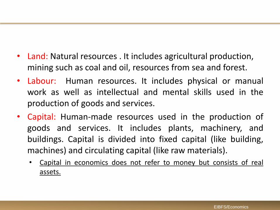
• An isoquant can be defined asa curve showing the variouscombinations of capital andlabor required to produce agiven quantity of a particularproduct, in the most efficientway.

• It reveals marginal rate oftechnical substitution oflabour for capital.

EIBFS/Economics

• An isoquant a curve showing the various combinations of capital and labor required to produce a product,

• An isocost line

represents the

various combinations

of capital and labour a

firm can buy for a

given expenditure.

EIBFS/Economics 11

ISOCOST

• An isocost line represents

the various combinations

of capital and labour a firm

can buy for a given

expenditure.

EIBFS/Economics 12

The Least-cost Process of Production

• When the isoquant istangential (Touching)bto the isocost this isthe least-cost process ofproduction.

EIBFS/Economics 13

Costs

• Cost is the total amount paid by a firm for the factors ofproduction used in the production process.

• Accountant VS Economics method of cost measurement.

• Accountant measures historical cost which is the price originally paid for the factors of production. (explicit costs).– Explicit cost (actual expenditure in monetary terms)

• Economists measures the opportunity cost. (explicit costs+ implicit costs).– Implicit costs (hidden cost) are estimated cost for which no

expenditure made.

EIBFS/Economics

14

Short-run and long-run Costs

• In the short run certain factors are fixed while others arevariable. (Both fixed and variable costs in the short run).

• In the long run, all the factors of production are variable. (Allcosts are variable.

EIBFS/Economics

Short-run and long-run Costs

• Fixed Costs (also called overhead or unavoidable costs) arethe costs that do not vary (change) with increase or decreaseof output.

• Example: rent on buildings, rent for equipment andwarehouses, loan payment.

• Fixed cost is incurred whether a unit of output is made or not.

EIBFS/Economics

• Variable Costs are the costs that vary with change in the levelof a firm’s output.

– Example: raw materials, wages of the operative staff andthe cost of fuel .

• Also called direct or avoidable costs.

• Variable costs are incurred only when a unit of output isproduced.

EIBFS/Economics

• Total cost (TC) is the total cost of producing aparticular level of output.

• Total cost is sum (total) of all fixed (TFC)and variablecosts(TVC)

• TC = TFC + TVC

EIBFS/Economics

EIBFS/Economics

• Average Fixed Cost (AFC) is calculated by:

• dividing total fixed cost divided by by the number of units produced (Q);

• AFC =TFC / Q

• Average Variable Cost (AVC) is calculated:

– by dividing total variable cost by the number of unitsproduced or,

• AVC = TVC / Q

• Marginal cost is the change in the total cost as a result of a change in output of one unit.

• MC = TC / Q

EIBFS/Economics

• Average Fixed Cost (AFC) is calculated by:

• dividing total fixed cost divided by by the number of units produced (Q);

• AFC =TFC / Q

• Average Variable Cost (AVC) is calculated:

– by dividing total variable cost by the number of unitsproduced or,

EIBFS/Economics

• Total Cost (TC): TC =TFC +TVC

• Average Fixed Cost (AFC):AFC =TFC / Q

• Average Variable Cost (AVC):AVC = TVC / Q

• Average Total Cost (ATC): ATC = TC/Q

• Marginal Cost (MC): MC = TC / Q

• Total cost: total cost of producinga particular level of output.

• Average Fixed Cost (AFC) total fixed cost divided by out put

• Average Variable Cost (AVC) totalvariable cost divided by out put

• Average Total Cost (ATC) is thecost per unit

• Marginal cost is the change in the total cost as a result of a change

in output of one unit.

EIBFS/Economics

• The average fixed cost

declines continuously as

output increases.

• The marginal cost (MC)

curve cuts the AVC and

ATC curves at theirminimum points

EIBFS/Economics

Long Run Average Cost and Economies of Scale

• In the long run all the factors of production are variable.

• The long-run average cost (LRAC) curve is the envelope to allthe short-run average cost curves.

• LRAC represents the lowest cost of producing different levelsof output when all factors can be varied.

EIBFS/Economics

24

Economies of scale

• Economies of scale refers to the fall in the long-run averagecost curve as output increases.

• Sources of economies of scale :

– Technical economies: (related to production; size of the plant orproduction unit etc) .

– Marketing Economies. (related to marketing, distribution,packaging etc)

– Financial economies (related to lower rates of interest, financing)

EIBFS/Economics

Economies of scope

• Economies of scope refers to reduction in average total (ATC) costs through a firm increasing the number of different goods it produces.

• Economies of scope exists when costs are spread over a range of products.

EIBFS/Economics

Diseconomies of Scale

• Diseconomies of scale refers to the rise in the long-runaverage cost curve as output increases.

• Sources of diseconomies of scale:

– Problems in managing the large firms, lack of coordination in planning, marketing, production,

– Poor motivation in workforce, low morale, industrial disputes,

EIBFS/Economics

• Economies of scale is referred as increasing returns to scale.(doubling of the input leads to more than doubling in theoutput).

• Diseconomies of scale is referred as decreasing returns toscale. (doubling of the input leads to less than doubling in theoutput).

• If (doubling of the input leads to exact doubling in the outputit is referred as constant returns to scale.)

EIBFS/Economics