Embed Size (px)
Citation preview
The “Checklist” > 2a. Estimation: Flexible Probabilities > Historical
Historical estimation with Flexible Probabilities
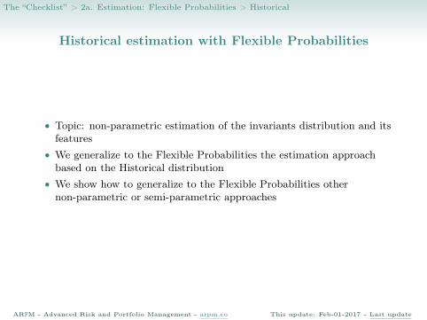
• Topic: non-parametric estimation of the invariants distribution and itsfeatures
• We generalize to the Flexible Probabilities the estimation approachbased on the Historical distribution
• We show how to generalize to the Flexible Probabilities othernon-parametric or semi-parametric approaches
ARPM - Advanced Risk and Portfolio Management - arpm.co This update: Feb-01-2017 - Last update
The “Checklist” > 2a. Estimation: Flexible Probabilities > HistoricalFrom historical distribution to Flexible Probabilities
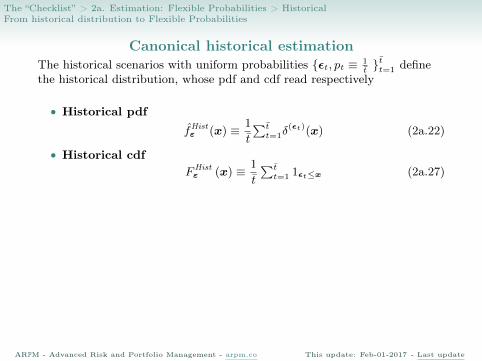
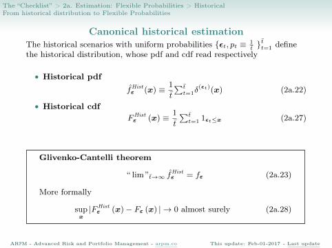
Canonical historical estimationThe historical scenarios with uniform probabilities {εt, pt ≡ 1
t}tt=1 define
the historical distribution, whose pdf and cdf read respectively
• Historical pdf
fHistε (x) ≡ 1
t
∑tt=1δ
(εt)(x) (2a.22)
• Historical cdfFHistε (x) ≡ 1
t
∑tt=1 1εt≤x (2a.27)
Glivenko-Cantelli theorem
“ lim ” t→∞ fHistε = fε (2a.23)
More formally
supx|FHistε (x)− Fε (x) | → 0 almost surely (2a.28)
ARPM - Advanced Risk and Portfolio Management - arpm.co This update: Feb-01-2017 - Last update
The “Checklist” > 2a. Estimation: Flexible Probabilities > HistoricalFrom historical distribution to Flexible Probabilities
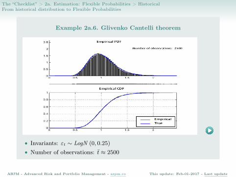
Example 2a.6. Glivenko Cantelli theorem
• Invariants: εt ∼ LogN (0, 0.25)
• Number of observations: t ≈ 2500
ARPM - Advanced Risk and Portfolio Management - arpm.co This update: Feb-01-2017 - Last update
The “Checklist” > 2a. Estimation: Flexible Probabilities > HistoricalFrom historical distribution to Flexible Probabilities
Generalization with Flexible Probabilities
The historical scenarios with Flexible Probabilities {εt, pt}tt=1 define theHistorical with Flexible Probabilities (HFP) distribution, whose pdf and cdfread respectively
• HFP pdffHFPε (x) ≡
∑tt=1 ptδ
(εt)(x) (2a.24)
• HFP cdfFHFPε (x) ≡
∑tt=1 pt1εt≤x (2a.26)
Generalized Glivenko-Cantelli theorem
“ lim ”ens(p)→∞ fHFPε = fε (2a.25)
where ens(p) is the Effective Number of Scenarios (2a.21).
ARPM - Advanced Risk and Portfolio Management - arpm.co This update: Feb-01-2017 - Last update
The “Checklist” > 2a. Estimation: Flexible Probabilities > HistoricalFrom historical distribution to Flexible Probabilities
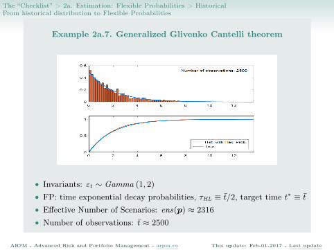
Example 2a.7. Generalized Glivenko Cantelli theorem
• Invariants: εt ∼ Gamma (1, 2)
• FP: time exponential decay probabilities, τHL ≡ t/2, target time t∗ ≡ t• Effective Number of Scenarios: ens(p) ≈ 2316
• Number of observations: t ≈ 2500
ARPM - Advanced Risk and Portfolio Management - arpm.co This update: Feb-01-2017 - Last update
The “Checklist” > 2a. Estimation: Flexible Probabilities > HistoricalFrom historical distribution to Flexible Probabilities
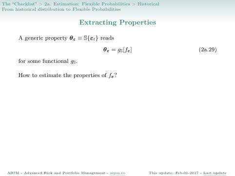
Extracting Properties
A generic property θε ≡ S{εt} reads
θε = gS[fε] (2a.29)
for some functional gS.
How to estimate the properties of fε?
Historical with Flexible Probabilities (HFP) estimate
θHFP
ε ≡ SHFP{ε} (2a.33)
fHFPε ≈
ens(p)→∞fε
gS
y ygS
θHFP
ε ≈ens(p)→∞
θε
(2a.35)
ARPM - Advanced Risk and Portfolio Management - arpm.co This update: Feb-01-2017 - Last update
The “Checklist” > 2a. Estimation: Flexible Probabilities > HistoricalFrom historical distribution to Flexible Probabilities
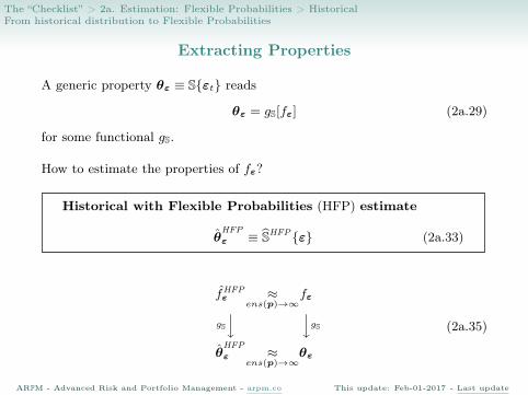
Extracting Properties
A generic property θε ≡ S{εt} reads
θε = gS[fε] (2a.29)
for some functional gS.
How to estimate the properties of fε?
Historical with Flexible Probabilities (HFP) estimate
θHFP
ε ≡ SHFP{ε} (2a.33)
fHFPε ≈
ens(p)→∞fε
gS
y ygS
θHFP
ε ≈ens(p)→∞
θε
(2a.35)
ARPM - Advanced Risk and Portfolio Management - arpm.co This update: Feb-01-2017 - Last update
The “Checklist” > 2a. Estimation: Flexible Probabilities > HistoricalKernel estimation with Flexible Probabilities
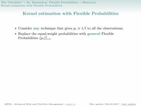
Kernel estimation with Flexible Probabilities
• Consider any technique that gives pt ≡ 1/t to all the observations;• Replace the equal-weight probabilities with general FlexibleProbabilities {pt}tt=1.
• Consider the kernel density estimate
fKerε (x) ≡ 1
t
∑tt=1δ
(εt)
h2 (x) (2a.55)
• Extend to the Kernel with Flexible Probabilities (KFP)pdf
fKFPε (x) ≡
∑tt=1ptδ
(εt)
h2 (x) (2a.57)
Example: KFP generalized mean
ARPM - Advanced Risk and Portfolio Management - arpm.co This update: Feb-01-2017 - Last update
The “Checklist” > 2a. Estimation: Flexible Probabilities > HistoricalKernel estimation with Flexible Probabilities
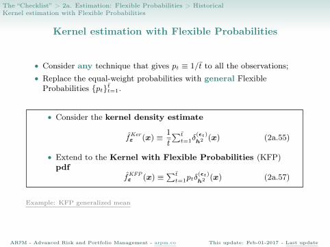
Kernel estimation with Flexible Probabilities
• Consider any technique that gives pt ≡ 1/t to all the observations;• Replace the equal-weight probabilities with general FlexibleProbabilities {pt}tt=1.
• Consider the kernel density estimate
fKerε (x) ≡ 1
t
∑tt=1δ
(εt)
h2 (x) (2a.55)
• Extend to the Kernel with Flexible Probabilities (KFP)pdf
fKFPε (x) ≡
∑tt=1ptδ
(εt)
h2 (x) (2a.57)
Example: KFP generalized mean
ARPM - Advanced Risk and Portfolio Management - arpm.co This update: Feb-01-2017 - Last update