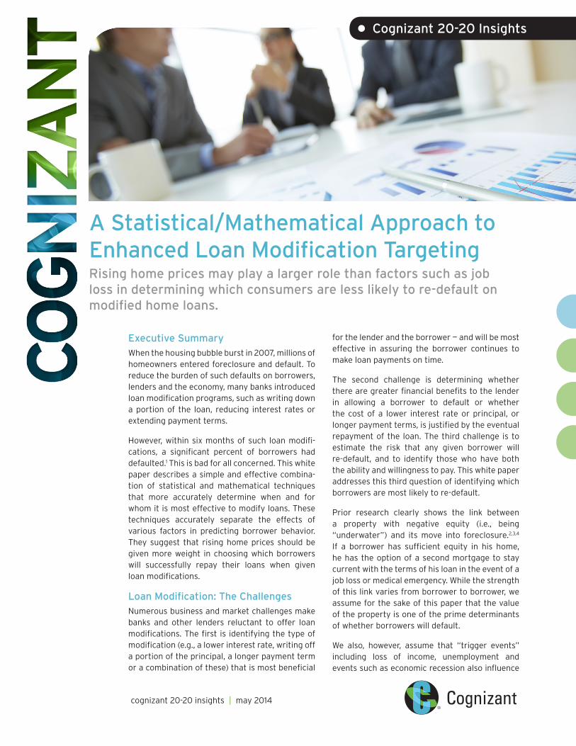
A Statistical/Mathematical Approach to Enhanced Loan Modification Targeting Rising home prices may play a larger role than factors such as job loss in determining which consumers are less likely to re-default on modified home loans.

Executive SummaryWhen the housing bubble burst in 2007, millions of homeowners entered foreclosure and default. To reduce the burden of such defaults on borrowers, lenders and the economy, many banks introduced loan modification programs, such as writing down a portion of the loan, reducing interest rates or extending payment terms.

However, within six months of such loan modifi-cations, a significant percent of borrowers had defaulted.1 This is bad for all concerned. This white paper describes a simple and effective combina-tion of statistical and mathematical techniques that more accurately determine when and for whom it is most effective to modify loans. These techniques accurately separate the effects of various factors in predicting borrower behavior. They suggest that rising home prices should be given more weight in choosing which borrowers will successfully repay their loans when given loan modifications.

Loan Modification: The Challenges Numerous business and market challenges make banks and other lenders reluctant to offer loan modifications. The first is identifying the type of modification (e.g., a lower interest rate, writing off a portion of the principal, a longer payment term or a combination of these) that is most beneficial

for the lender and the borrower — and will be most effective in assuring the borrower continues to make loan payments on time.

The second challenge is determining whether there are greater financial benefits to the lender in allowing a borrower to default or whether the cost of a lower interest rate or principal, or longer payment terms, is justified by the eventual repayment of the loan. The third challenge is to estimate the risk that any given borrower will re-default, and to identify those who have both the ability and willingness to pay. This white paper addresses this third question of identifying which borrowers are most likely to re-default.

Prior research clearly shows the link between a property with negative equity (i.e., being “underwater”) and its move into foreclosure.2,3,4 If a borrower has sufficient equity in his home, he has the option of a second mortgage to stay current with the terms of his loan in the event of a job loss or medical emergency. While the strength of this link varies from borrower to borrower, we assume for the sake of this paper that the value of the property is one of the prime determinants of whether borrowers will default.

We also, however, assume that “trigger events” including loss of income, unemployment and events such as economic recession also influence

• Cognizant 20-20 Insights

cognizant 20-20 insights | may 2014

2

the default decision. So do borrower attributes such as the borrower’s credit score, age, education, marital status and type of loan (e.g., the interest rate, adjustable vs. fixed, etc.)

Our Analytical Approach

Performance data on the aftermath of loan modi-fications is scarce. However, using data about the customer’s behavior before his loan was modified is technically equivalent to using post-loan-mod-ification data to determine the probability he will default.

We perform our analysis by estimating a second order Markov chain/transition matrix. This differs from traditional prediction techniques in that it considers only the borrower’s most recent state (i.e., his demonstrated willingness and ability to pay) rather than his long-term history in order to predict future behavior and thus what sort of loan modification, if any, he should receive. Our hypothesis, which has been demonstrated by application of this technique, is that this analysis produces more accurate results than traditional methods such as credit scoring or long-term analysis of payment behaviors.

Conditional probabilities can be estimated by either multinomial logistic regression (which assumes the same set of variables influence all state equations) or binomial logistic regression (and rescaling so that the range of probabilities add up to 1 by applying the Begg-Gray method).5 Either of these techniques allows the effects of loans that end early due to prepayment to be separated from those that end early due to default.

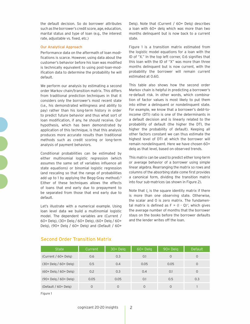
Let’s illustrate with a numerical example. Using loan level data we build a multinomial logistic model. The dependent variables are (Current / 60+ Delq), (30+ Delq / 60+ Delq), (60+ Delq / 60+ Delq), (90+ Delq / 60+ Delq) and (Default / 60+

Delq). Note that (Current / 60+ Delq) describes a loan with 60+ delq which was more than two months delinquent but is now back to a current state.

Figure 1 is a transition matrix estimated from the logistic model equations for a loan with the ID of “X.” In the top left corner, 0.6 signifies that this loan with the ID of “X” was more than three months delinquent but is now current, with the probability the borrower will remain current estimated at 0.60.

This table also shows how the second order Markov chain is helpful in predicting a borrower’s re-default risk. In other words, which combina-tion of factor values is most likely to put them into either a delinquent or nondelinquent state. For example, we know that a borrower’s debt-to-income (DTI) ratio is one of the determinants in a default decision and is linearly related to the probability of default (the higher the DTI, the higher the probability of default). Keeping all other factors constant we can thus estimate the highest level of DTI at which the borrower will remain nondelinquent. Here we have chosen 60+ delq as that level, based on observed trends.

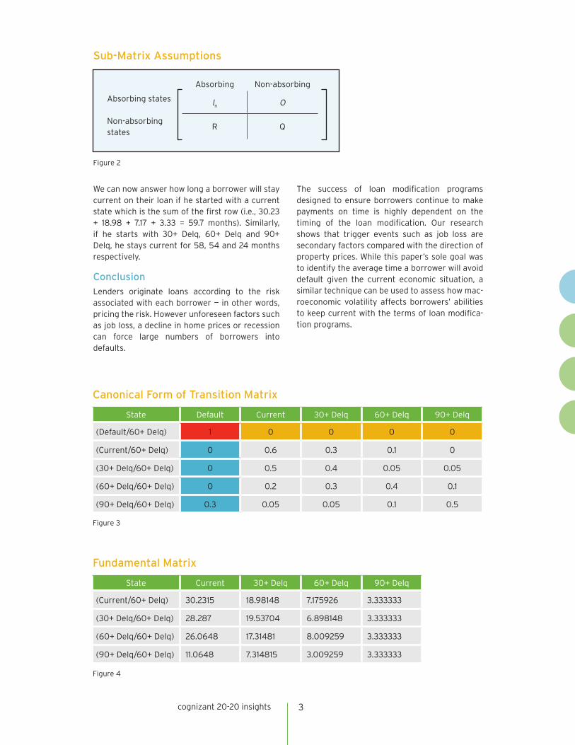
This matrix can be used to predict either long-term or average behavior of a borrower using simple linear algebra. Rearranging the matrix so rows and columns of the absorbing state come first provides a canonical form, dividing the transition matrix into four sub-matrices (as shown in Figure 2).

Note that In is the square identity matrix if there is more than one observing state. Otherwise, the scalar and 0 is zero matrix. The fundamen-tal matrix is defined as F = (I - Q)-1, which gives the average number of months that the borrower stays on the books before the borrower defaults and the lender writes off the loan.

cognizant 20-20 insights

Second Order Transition Matrix

Figure 1

State Current 30+ Delq 60+ Delq 90+ Delq Default

(Current / 60+ Delq) 0.6 0.3 0.1 0 0

(30+ Delq / 60+ Delq) 0.5 0.4 0.05 0.05 0

(60+ Delq / 60+ Delq) 0.2 0.3 0.4 0.1 0

(90+ Delq / 60+ Delq) 0.05 0.05 0.1 0.5 0.3

(Default / 60+ Delq) 0 0 0 0 1

3cognizant 20-20 insights

We can now answer how long a borrower will stay current on their loan if he started with a current state which is the sum of the first row (i.e., 30.23 + 18.98 + 7.17 + 3.33 = 59.7 months). Similarly, if he starts with 30+ Delq, 60+ Delq and 90+ Delq, he stays current for 58, 54 and 24 months respectively.

Conclusion Lenders originate loans according to the risk associated with each borrower — in other words, pricing the risk. However unforeseen factors such as job loss, a decline in home prices or recession can force large numbers of borrowers into defaults.

The success of loan modification programs designed to ensure borrowers continue to make payments on time is highly dependent on the timing of the loan modification. Our research shows that trigger events such as job loss are secondary factors compared with the direction of property prices. While this paper’s sole goal was to identify the average time a borrower will avoid default given the current economic situation, a similar technique can be used to assess how mac-roeconomic volatility affects borrowers’ abilities to keep current with the terms of loan modifica-tion programs.

Sub-Matrix Assumptions

Figure 2

Absorbing Non-absorbing

Absorbing states In O

Non-absorbing states

R Q

Canonical Form of Transition Matrix

Fundamental Matrix

Figure 3

Figure 4

State Default Current 30+ Delq 60+ Delq 90+ Delq

(Default/60+ Delq) 1 0 0 0 0

(Current/60+ Delq) 0 0.6 0.3 0.1 0

(30+ Delq/60+ Delq) 0 0.5 0.4 0.05 0.05

(60+ Delq/60+ Delq) 0 0.2 0.3 0.4 0.1

(90+ Delq/60+ Delq) 0.3 0.05 0.05 0.1 0.5

State Current 30+ Delq 60+ Delq 90+ Delq

(Current/60+ Delq) 30.2315 18.98148 7.175926 3.333333

(30+ Delq/60+ Delq) 28.287 19.53704 6.898148 3.333333

(60+ Delq/60+ Delq) 26.0648 17.31481 8.009259 3.333333

(90+ Delq/60+ Delq) 11.0648 7.314815 3.009259 3.333333

About CognizantCognizant (NASDAQ: CTSH) is a leading provider of information technology, consulting, and business process out-sourcing services, dedicated to helping the world’s leading companies build stronger businesses. Headquartered in Teaneck, New Jersey (U.S.), Cognizant combines a passion for client satisfaction, technology innovation, deep industry and business process expertise, and a global, collaborative workforce that embodies the future of work. With over 75 development and delivery centers worldwide and approximately 178,600 employees as of March 31, 2014, Cognizant is a member of the NASDAQ-100, the S&P 500, the Forbes Global 2000, and the Fortune 500 and is ranked among the top performing and fastest growing companies in the world. Visit us online at www.cognizant.com or follow us on Twitter: Cognizant.

World Headquarters500 Frank W. Burr Blvd.Teaneck, NJ 07666 USAPhone: +1 201 801 0233Fax: +1 201 801 0243Toll Free: +1 888 937 3277Email: inquiry@cognizant.com

European Headquarters1 Kingdom StreetPaddington CentralLondon W2 6BDPhone: +44 (0) 20 7297 7600Fax: +44 (0) 20 7121 0102Email: infouk@cognizant.com

India Operations Headquarters#5/535, Old Mahabalipuram RoadOkkiyam Pettai, ThoraipakkamChennai, 600 096 IndiaPhone: +91 (0) 44 4209 6000Fax: +91 (0) 44 4209 6060Email: inquiryindia@cognizant.com

© Copyright 2014, Cognizant. All rights reserved. No part of this document may be reproduced, stored in a retrieval system, transmitted in any form or by any means, electronic, mechanical, photocopying, recording, or otherwise, without the express written permission from Cognizant. The information contained herein is subject to change without notice. All other trademarks mentioned herein are the property of their respective owners.

About the Authors Mahesh Hunasikatti is a Senior Associate with Cognizant Analytics. With wide experience applying statistics business consulting and analytics in mortgage retail banking, financial and insurance industries, Mahesh has delivered analytics services in the areas of mortgage product develop-ment, product pricing, claims and fraud management in both the banking and insurance industries. He holds an M.Sc. from the University of Agricultural Sciences, Bangalore. Mahesh can be reached at Mahesh.Hunasikatti@cognizant.com.

Manivannan Karuppusamy is a Manager with Cognizant Analytics. He has 11 years of experience in analytics and has worked extensively in the mortgage domain for the last few years. Manivannan is responsible for modeling and development, as well as testing and research, for U.S. mortgage products such as pre-payment risk, credit risk and collateral risk-fraud. He can be reached at Manivannan.Karuppusamy2@cognizant.com.

Footnotes1 OCC and OTS Mortgage Metrics Report: Disclosure of National Bank and Federal Thrift Mortgage, Office

of the Comptroller of the Currency and Office of Thrift Supervision (OCC and OTS), 2008. 2 Foster, Chester, and Robert Van Order, “An Option-Based Model of Mortgage Default,”

Housing Finance Review 3 (4): 351–72; 1984.3 Kau, James B., Donald C. Keenan, and Taewon Kim, “Transaction Costs, Suboptimal Termination and

Default Probabilities,” Journal of the American Estate and Urban Economics Association 21 (3): 247–63; 1993.

4 Vandell, Kelly D., “How Ruthless Is Mortgage Default? A Review and Synthesis of the Evidence,” Journal of Housing Research 6 (2): 245–62; 1995.

5 Begg, C.B. and R. Gray, “Calculation of Polychotomous Logistic Regression Parameters Using, Individualized Regressions,” Biometrika, 71(1):11-18; 1984.

AcknowledgementThe authors would like to thank Rajendra Anjanappa for his invaluable contributions and support in the development of this white paper.

References

• Loan Data, Third Quarter 2008, Office of Thrift Supervision, Department of the Treasury, Washington, D.C.

• Pearson’s, An Addison-Wesley product, “MARKOV CHAINS,” 2003, http://www.aw-bc.com/greenwell/markov.pdf.