Hodrick-Prescott filter
• Assume that the series yt is the sum of the growt component gt and acyclical component ct
yt = ct + gt for t = 1, . . . , T
• The growth component gt varies smoothly over time
• The cyclical component ct is in average equal to zero
• Assume taht measure of smoothness of {gt} path is the sum of squares ofits second differances
Macroeconometrics, WNE UW, Copyright c©2007 by Jerzy Mycielski 1

• The to filter ct and gt we have to solve following maximization problem
min{gt}T
t=−1
{T∑
t=1
c2t + λ
T∑t=1
∆2gt
}
where ct = yt − gt
• λ is a positive number which panelizes the variability in growth componentseries
• The larger is λ the smoother is the solution, for λ → ∞ the solution of theproblem is the OLS fit of linear trend
• Hodrick and Prescott suggested to use λ = 1600 for quarterly data.Rawn and Uhlig (2002) shown that λ should be proprtional to 4 powerof frequency observation rations.
Macroeconometrics, WNE UW, Copyright c©2007 by Jerzy Mycielski 2

• This implies λ = 6.25 for annual data and 129600 for monthly data
• The Hodrick-Prescott filter can be derived as special case of Kalman filterif we assume:
– vector of state zt = [ct, gt]– transition equation is of the form:
ct = ε1t
gt = gt−1 + ε2t
– Random components ε1t and ε2t are NID and independ of each other
εt ∼ N
(0,
[σ2
1 00 σ2
2
])
Macroeconometrics, WNE UW, Copyright c©2007 by Jerzy Mycielski 3

– Smoothing parameter is equal to ratio of variances of ε1 and ε2
λ =σ2
1
σ22
• Typical application of Hodrick-Prescott filter: filtering the output gap
Macroeconometrics, WNE UW, Copyright c©2007 by Jerzy Mycielski 4

Markov chain definition
• Values of random variable Xn are in finite set {s1, s2, . . . , sr}
• Finite Markov chain
Pr (Xn = j|X0 = i0, X1 = i1, . . . , Xn−1 = in−1) = P (Xn = j|Xn−1 = i)
• This process has a short memory, transition probability only depends onthe state of the process in previous period
• Finite homogenous Markov chain has a following property:
P (Xn = j|Xn−1 = i) = P (Xn+s = j|Xn+s−1 = i) = pij
Macroeconometrics, WNE UW, Copyright c©2007 by Jerzy Mycielski 5

• For homogenous Markov chain, transition probabilities do not change overtime
Macroeconometrics, WNE UW, Copyright c©2007 by Jerzy Mycielski 6

Matrix of transition probabilities
• Matrix of transition probabilities has a following form:
P =
p11 p12 · · · p1r
p21 p22 · · · p2r... ... ...
pr1 pr2 · · · prr
• pij has to satisfy following properties:
r∑
j=1
pij = 1
pij ≥ 0
Macroeconometrics, WNE UW, Copyright c©2007 by Jerzy Mycielski 7

Marginal distribution of Markov chain
• Marginal probability distribution of the Markov chain state:
dnj = Pr (Xn = j)
which can be denoted as a vector:
dn =[
dn1 dn2 · · · dnr
]
where:r∑
i=j
dnj = 1
dnj ≥ 0
Macroeconometrics, WNE UW, Copyright c©2007 by Jerzy Mycielski 8

• Marginal probabilities for the Markov chain can be calculated as follows
dnj = Pr (Xn = j)
= Pr (Xn = j|Xn−1 = 1) Pr (Xn−1 = 1) + . . . + Pr (Xn = j|Xn−1 = r) Pr (Xn−1 = r)
=r∑
i=1
Pr (Xn = i|Xn−1 = i) Pr (Xn−1 = i) =r∑
i=1
dn−1,ipij
• This formula can be written using matrix notation:
dn = dn−1 P
• Recursively repeating this transformation we get:
dn = d0 P n
Macroeconometrics, WNE UW, Copyright c©2007 by Jerzy Mycielski 9

P n =
p(n)11 p
(n)12 · · · p
(n)1r
p(n)21 p
(n)22 · · · p
(n)2r... ... ...
p(n)r1 p
(n)r2 · · · p
(n)rr
Macroeconometrics, WNE UW, Copyright c©2007 by Jerzy Mycielski 10

Stationary distribution of Markov chain
• Stationary distribution of Markow chain is such vector d, for which:
d = dP
• This is the charcteristic equation for matrix P . Vector d is left eigenvectorof matrix P related to eigenvalue λ1 = 1.
• It is possible to prove that each matrix P has at least one d satifyng thisequation.
Macroeconometrics, WNE UW, Copyright c©2007 by Jerzy Mycielski 11
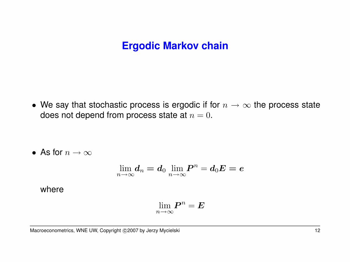
Ergodic Markov chain
• We say that stochastic process is ergodic if for n → ∞ the process statedoes not depend from process state at n = 0.
• As for n →∞lim
n→∞dn = d0 lim
n→∞P n = d0E = e
where
limn→∞
P n = E
Macroeconometrics, WNE UW, Copyright c©2007 by Jerzy Mycielski 12

• The Markov chain is ergotic only if for every d0
d0E = e
r∑
j=1
ej = 1
• This is only possible if all rows of E is equal
• Vector e is called the steady state of Markow chain
• As e is the only stationary distribution of ergodic Markov chain
• Therfore steady state for ergodic Markov chain can be found from followingsystem of equations: {
eP = ee1 = 1
Macroeconometrics, WNE UW, Copyright c©2007 by Jerzy Mycielski 13

Estimation of transition probabilities, individual level data
• Estimation with ML
• Likelihood function
Pr [n (1) , . . . , n (T )] =T∏
t=1
∏
i∈S
ni (t− 1)!∏
j∈S
nij (t)!
∏
j∈S
pnij(t)
ijt
where n (t) = [n1 (t) , . . . , nr (t)] is the vector of empirical counts for states
• The way we estimate depend on whether we assume homogeneity.
Macroeconometrics, WNE UW, Copyright c©2007 by Jerzy Mycielski 14
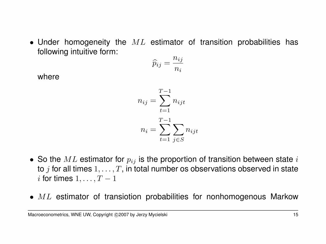
• Under homogeneity the ML estimator of transition probabilities hasfollowing intuitive form:
p̂ij =nij
ni
where
nij =T−1∑t=1
nijt
ni =T−1∑t=1
∑
j∈S
nijt
• So the ML estimator for pij is the proportion of transition between state ito j for all times 1, . . . , T , in total number os observations observed in statei for times 1, . . . , T − 1
• ML estimator of transiotion probabilities for nonhomogenous Markow
Macroeconometrics, WNE UW, Copyright c©2007 by Jerzy Mycielski 15
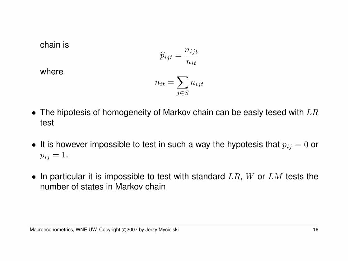
chain isp̂ijt =
nijt
nit
wherenit =
∑
j∈S
nijt
• The hipotesis of homogeneity of Markov chain can be easly tesed with LRtest
• It is however impossible to test in such a way the hypotesis that pij = 0 orpij = 1.
• In particular it is impossible to test with standard LR, W or LM tests thenumber of states in Markov chain
Macroeconometrics, WNE UW, Copyright c©2007 by Jerzy Mycielski 16

Estimation of transition probabilities, aggregated data
• For aggregated data we only observe the numbers of units (or fractions)observed in given states in time t
• Conditional expected value of the number of observations in state j in timet from ni observation, which were obseved to be in state i in time t − 1 isequal to:
E [nij (t)|ni (t− 1)] = ni (t− 1) pij
• From independence of transition we obtain
E [nj (t)|N (t− 1)] =∑
i∈S
ni (t− 1) pij = N (t− 1) pj
Macroeconometrics, WNE UW, Copyright c©2007 by Jerzy Mycielski 17

where pj is j-th column of the matrix of transition probabilities and rowvector N (t− 1) = [n1 (t) , . . . , nr (t)] is a vector of numbers of units beingin each state
• Denote as εit = ni (t)−∑
ni (t− 1) pij, and the we obtain
nj (t) =∑
i∈S
ni (t− 1) pij + εit = N (t− 1)pj + εit for j ∈ S
where εt satisfyE [εt|N (t− 1)] = 0
• This model can be written as
N (t) = N (t− 1) P + εt
andN (t)1 = N (t− 1)1
Macroeconometrics, WNE UW, Copyright c©2007 by Jerzy Mycielski 18

• As the number of unit should be constant over time the following addtionalrestriction should be valid
N (t)1 = N (t− 1) 1 = N
where N is the total number of units obeserved
• This model can be estimated be OLS applied to each equation or moreefficiently with GMM or GLS apllied to all equation
• The major problem in estimation of this model is related the fact that wehave to impose restriction that all the coefficients pij > 0
Macroeconometrics, WNE UW, Copyright c©2007 by Jerzy Mycielski 19

Marcov switching models
• Assume that we there are two regimes (e.g. recession and expansion)
• Each of the regimes is decribed with the different model
• We can not directly identify the regime in place in time t
• Denote regime by St ∈ {0, 1}
• Assume thatE (yt|St) = α0 + α1St + βxt
• The regimes differ by constant term α1
Macroeconometrics, WNE UW, Copyright c©2007 by Jerzy Mycielski 20

• The general case is if the transition probabilities can be influenced by someexogenous variables
• Transition probabilities are then given by:
P t =[
qt 1− qt
pt 1− pt
]
where
qt = Pr (St = 0|St−1 = 0) = Φ (δxt)
pt = Pr (St = 1|St−1 = 1) = Φ (γxt)
• With this kind of model we can:
– filter the probabilities states St (e.g. recession, expansion)
Macroeconometrics, WNE UW, Copyright c©2007 by Jerzy Mycielski 21

– distinguish two channels of influence: the influence on the probabilityof states and the direct influence on expected value of the dependentvariable
Macroeconometrics, WNE UW, Copyright c©2007 by Jerzy Mycielski 22
Recommended