Investigation Of
Performance Problems With
Event Detection Systems
Ed Roehl, John Cook, Ruby Daamen, and Uwe Mundry
Advanced Data Mining International, LLC
Greenville, South Carolina

Background
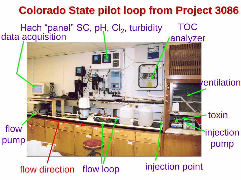
Colorado State pilot loop from Project 3086
flow loop
TOC
analyzer Hach “panel” SC, pH, Cl2, turbidity
flow
pump
data acquisition
toxin
ventilation
injection point
injection
pump
flow direction
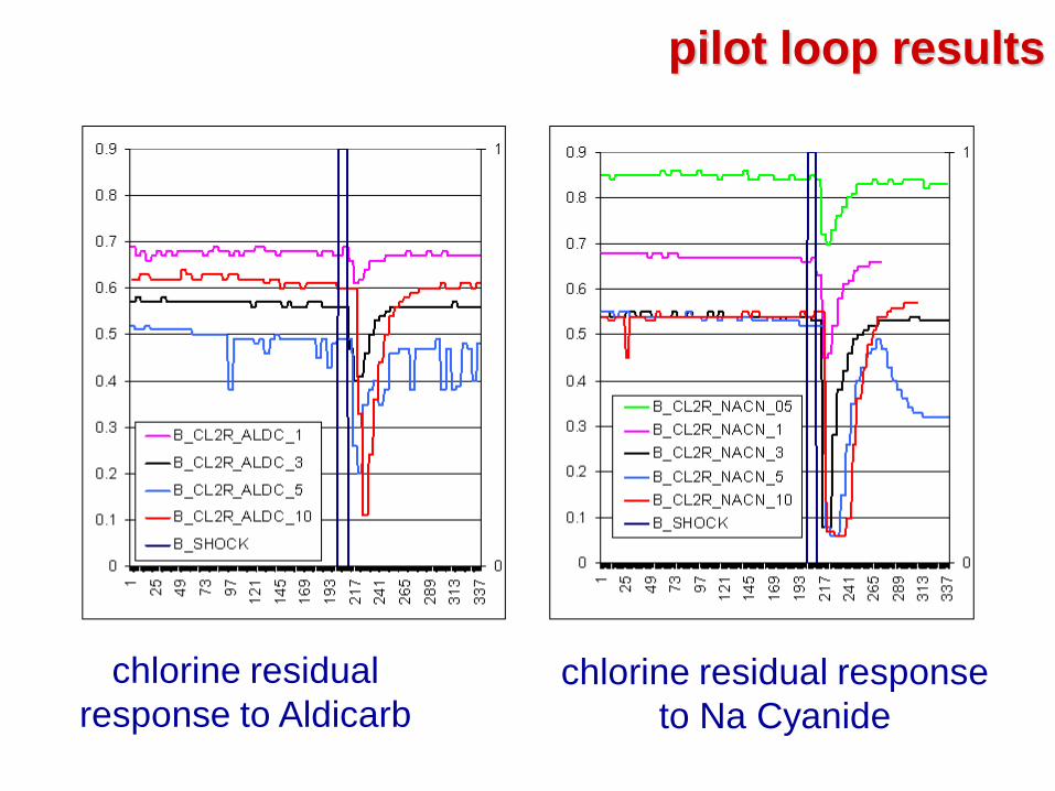
pilot loop results
chlorine residual
response to Aldicarb
chlorine residual response
to Na Cyanide
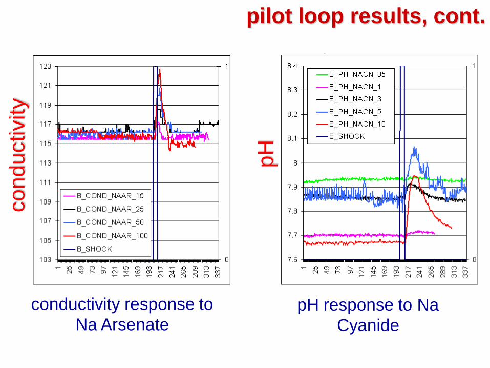
pilot loop results, cont. conductivity
pH
conductivity response to
Na Arsenate
pH response to Na
Cyanide
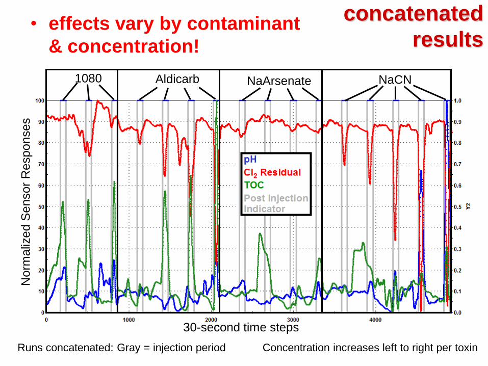
concatenated
results • effects vary by contaminant
& concentration!
NaArsenate Aldicarb NaCN 1080
30-second time steps
Norm
aliz
ed S
ensor
Responses
Runs concatenated: Gray = injection period Concentration increases left to right per toxin
Lab Data
Real Data
This slide shows the difference between
test results and reality
Danger!!!
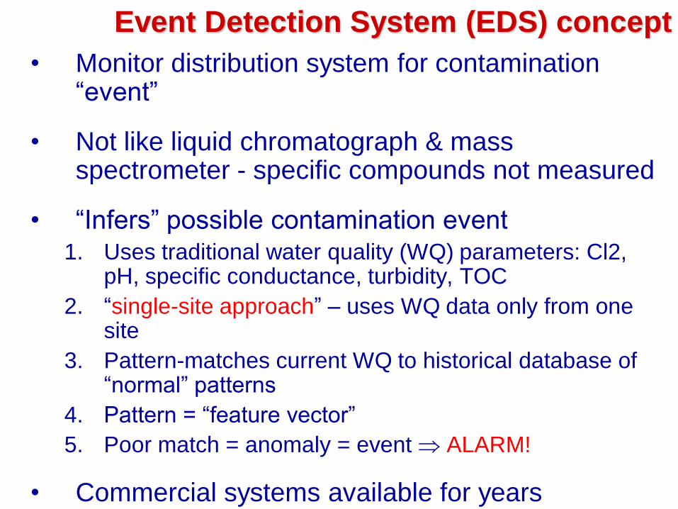
Event Detection System (EDS) concept
• Monitor distribution system for contamination “event”
• Not like liquid chromatograph & mass spectrometer - specific compounds not measured
• “Infers” possible contamination event 1. Uses traditional water quality (WQ) parameters: Cl2,
pH, specific conductance, turbidity, TOC
2. “single-site approach” – uses WQ data only from one site
3. Pattern-matches current WQ to historical database of “normal” patterns
4. Pattern = “feature vector”
5. Poor match = anomaly = event ALARM!
• Commercial systems available for years
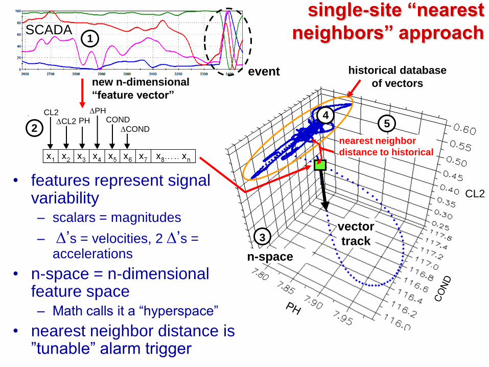
single-site “nearest
neighbors” approach
CL2
vector
track
PH
DCOND
COND DCL2
CL2 DPH
SCADA
event
n-space
historical database
of vectors
nearest neighbor
distance to historical
1
2
3
4 5
new n-dimensional
“feature vector”
• features represent signal variability – scalars = magnitudes
– D’s = velocities, 2 D’s = accelerations
• n-space = n-dimensional feature space – Math calls it a “hyperspace”
• nearest neighbor distance is ”tunable” alarm trigger
single-site approach - BIG assumption
• WQ variability caused by real contamination
events is different from variability caused by
normal operations.
– “normal vectors” relegated to limited regions of
n-space!
– “event vectors” appear where normal vectors do
not!
Water Research
Foundation Project 4182
“Interpreting Real-Time Online
Monitoring Data for Water Quality
Event Detection”
Project 4182
• Goal – improve EDS reliability
– Too many false positives/alarms
– Too many false negatives when testing with
“simulated events”
• How? - incorporate operations and hydraulic
data into EDS
• Technical Approach
1. Determine causes of false positives and negatives
2. Find new approach incorporating operations and
hydraulic data
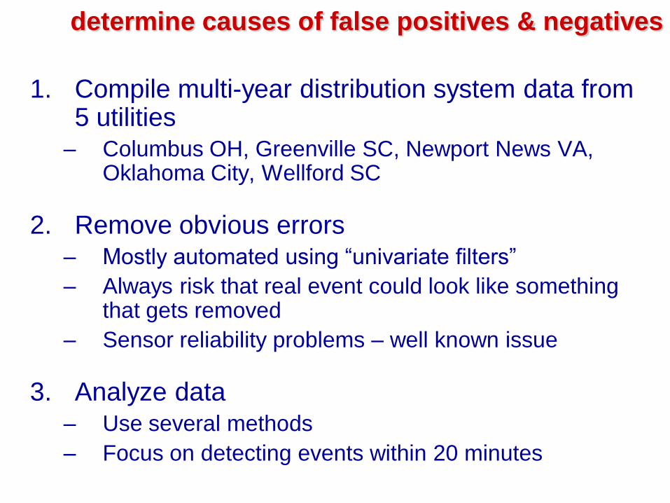
determine causes of false positives & negatives
1. Compile multi-year distribution system data from 5 utilities
– Columbus OH, Greenville SC, Newport News VA, Oklahoma City, Wellford SC
2. Remove obvious errors – Mostly automated using “univariate filters”
– Always risk that real event could look like something that gets removed
– Sensor reliability problems – well known issue
3. Analyze data – Use several methods
– Focus on detecting events within 20 minutes
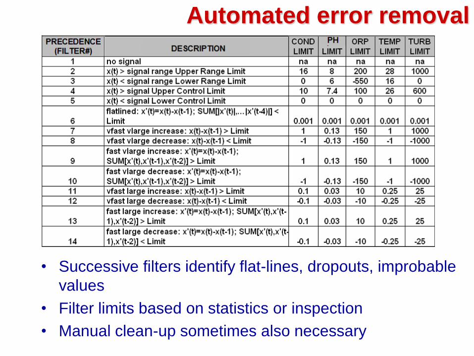
Automated error removal
• Successive filters identify flat-lines, dropouts, improbable
values
• Filter limits based on statistics or inspection
• Manual clean-up sometimes also necessary
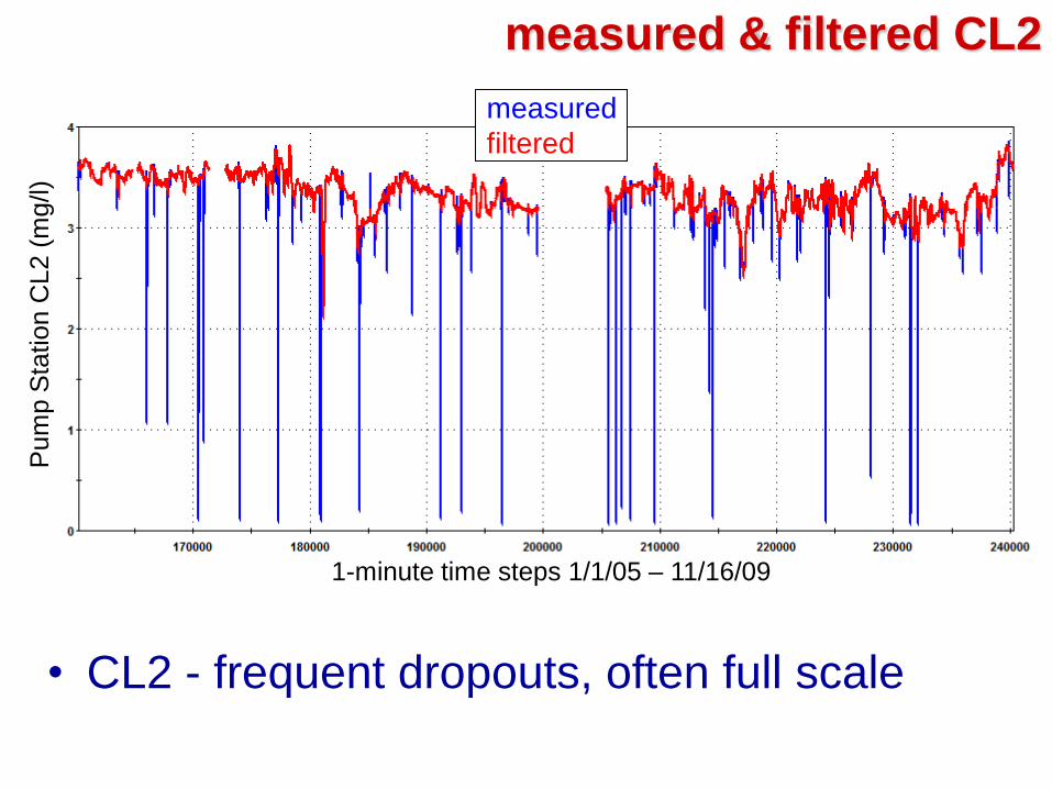
measured & filtered CL2
• CL2 - frequent dropouts, often full scale
Pum
p S
tation C
L2 (
mg/l)
measured
filtered
1-minute time steps 1/1/05 – 11/16/09
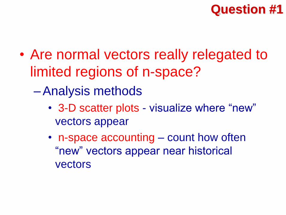
Question #1
• Are normal vectors really relegated to
limited regions of n-space?
– Analysis methods
• 3-D scatter plots - visualize where “new”
vectors appear
• n-space accounting – count how often
“new” vectors appear near historical
vectors
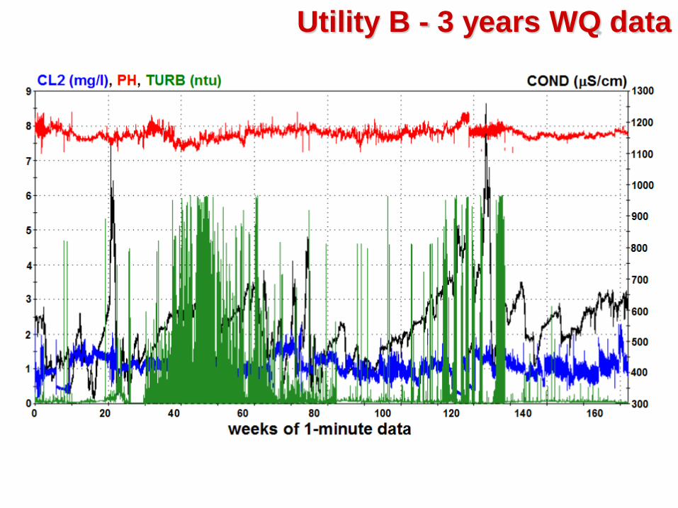
Utility B - 3 years WQ data
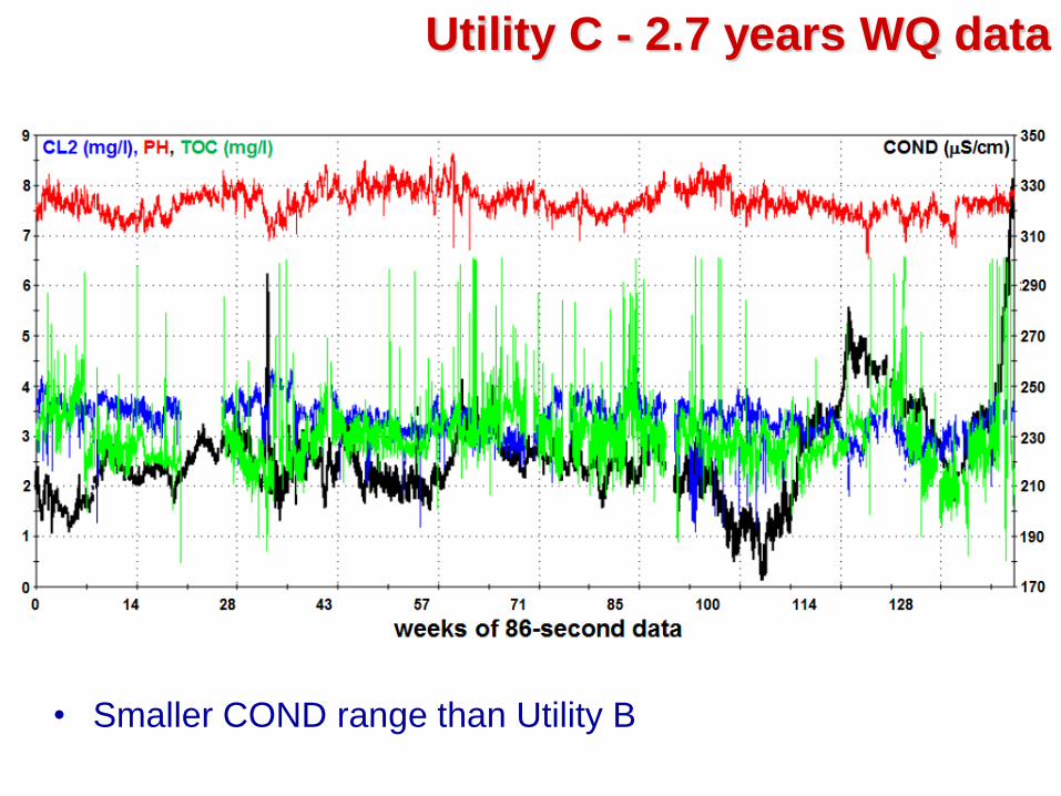
Utility C - 2.7 years WQ data
• Smaller COND range than Utility B
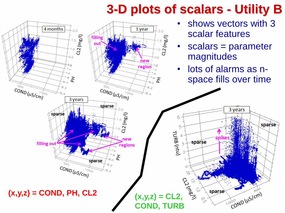
3-D plots of scalars - Utility B • shows vectors with 3
scalar features
• scalars = parameter magnitudes
• lots of alarms as n-space fills over time
(x,y,z) = COND, PH, CL2 (x,y,z) = CL2,
COND, TURB
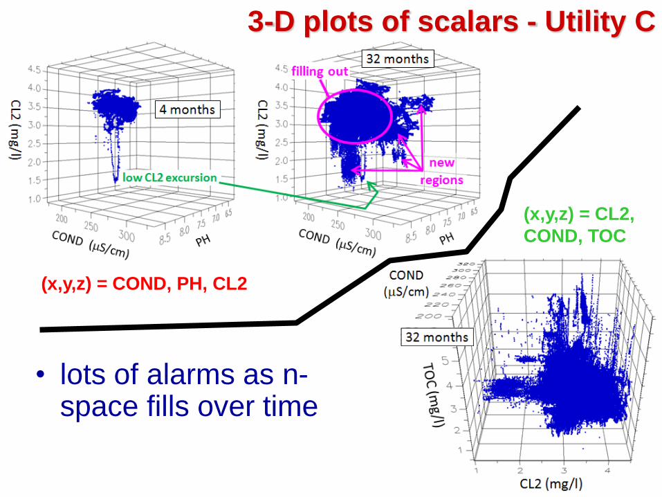
3-D plots of scalars - Utility C
(x,y,z) = CL2,
COND, TOC
(x,y,z) = COND, PH, CL2
• lots of alarms as n-space fills over time
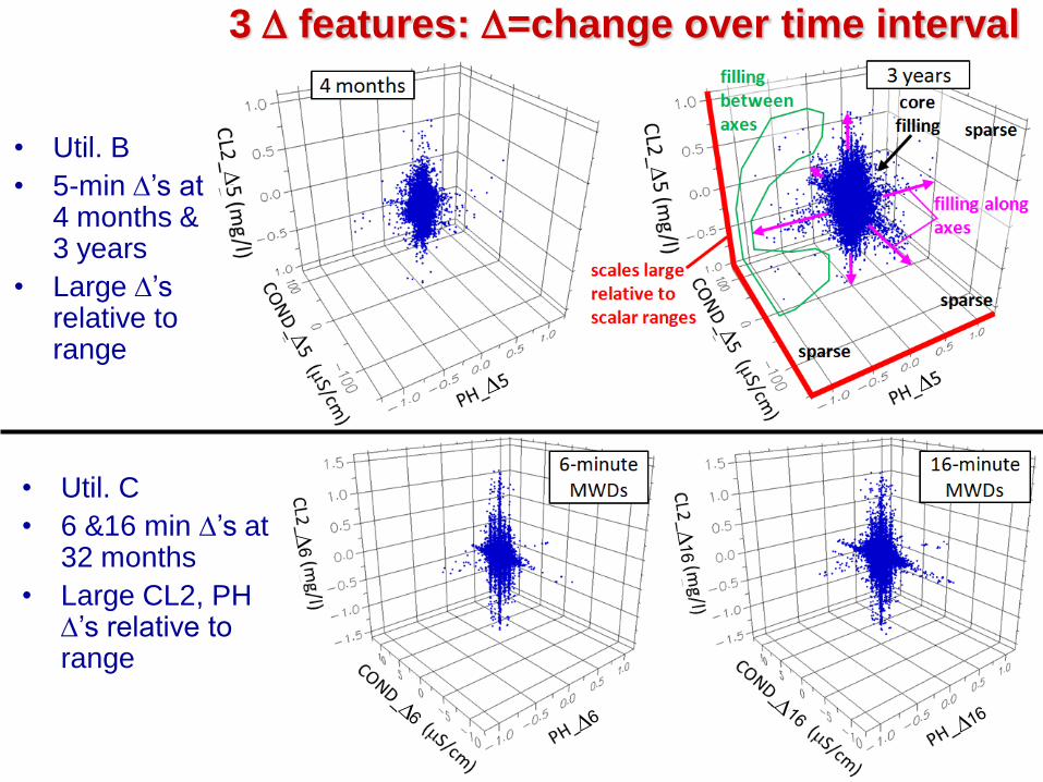
3 D features: D=change over time interval
• Util. C
• 6 &16 min D’s at 32 months
• Large CL2, PH D’s relative to range
• Util. B
• 5-min D’s at 4 months & 3 years
• Large D’s relative to range
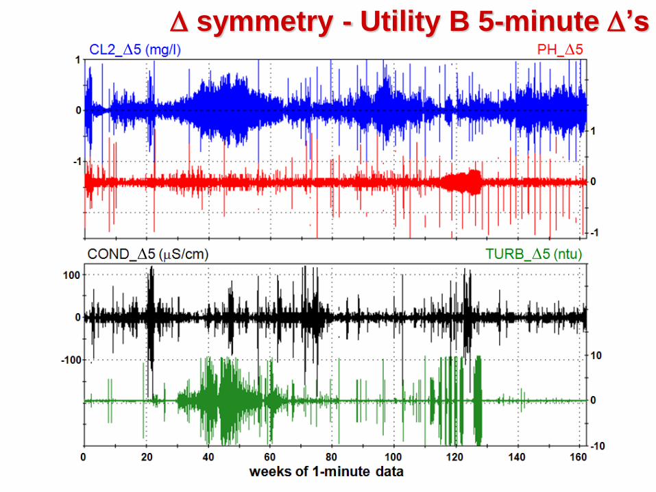
D symmetry - Utility B 5-minute D’s D D
D D
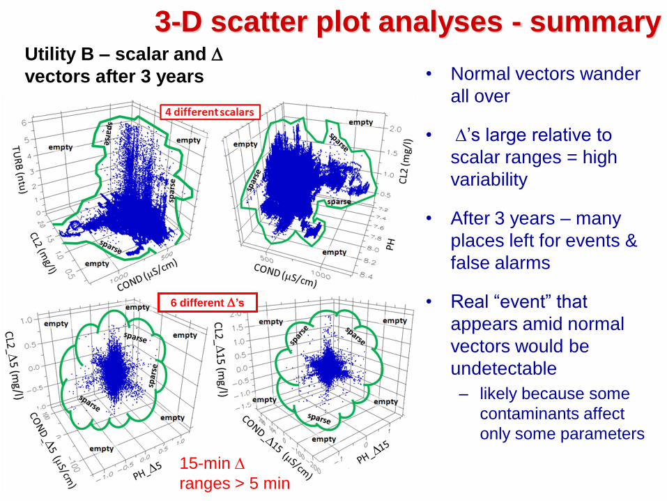
3-D scatter plot analyses - summary
• Normal vectors wander
all over
• D’s large relative to
scalar ranges = high
variability
• After 3 years – many
places left for events &
false alarms
• Real “event” that
appears amid normal
vectors would be
undetectable
– likely because some
contaminants affect
only some parameters
Utility B – scalar and D
vectors after 3 years
6 different D’s
15-min D
ranges > 5 min
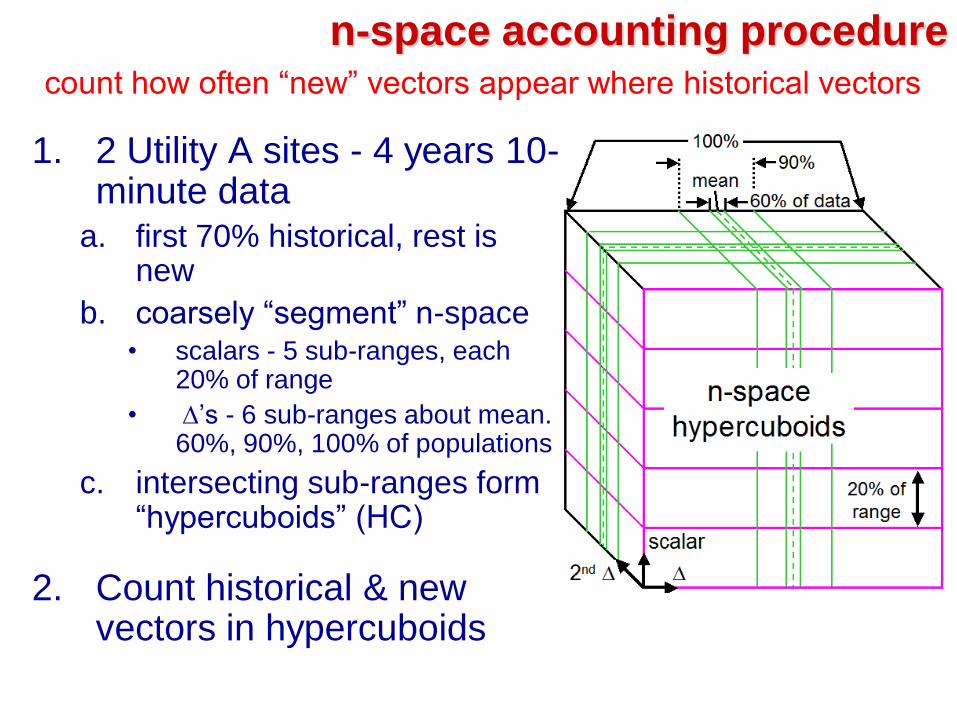
n-space accounting procedure
1. 2 Utility A sites - 4 years 10-minute data
a. first 70% historical, rest is new
b. coarsely “segment” n-space • scalars - 5 sub-ranges, each
20% of range
• D’s - 6 sub-ranges about mean. 60%, 90%, 100% of populations
c. intersecting sub-ranges form “hypercuboids” (HC)
2. Count historical & new vectors in hypercuboids
count how often “new” vectors appear where historical vectors
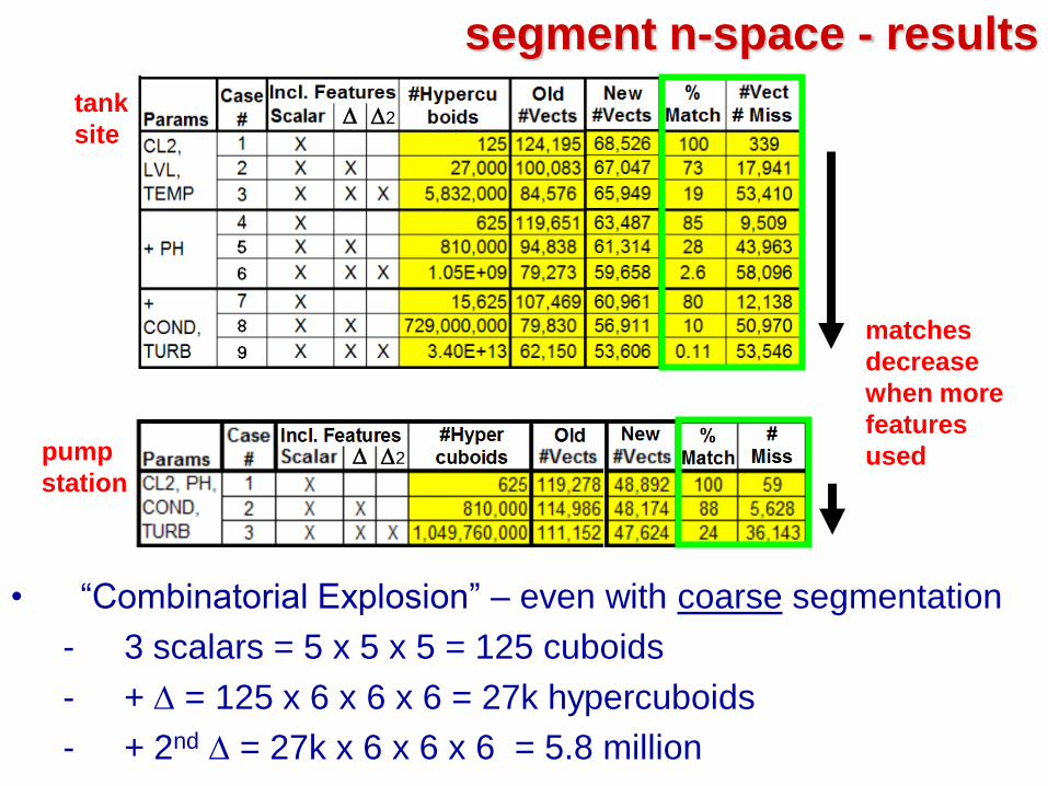
segment n-space - results
tank
site
• “Combinatorial Explosion” – even with coarse segmentation
- 3 scalars = 5 x 5 x 5 = 125 cuboids
- + D = 125 x 6 x 6 x 6 = 27k hypercuboids
- + 2nd D = 27k x 6 x 6 x 6 = 5.8 million
pump
station
D D2
D D2
matches
decrease
when more
features
used
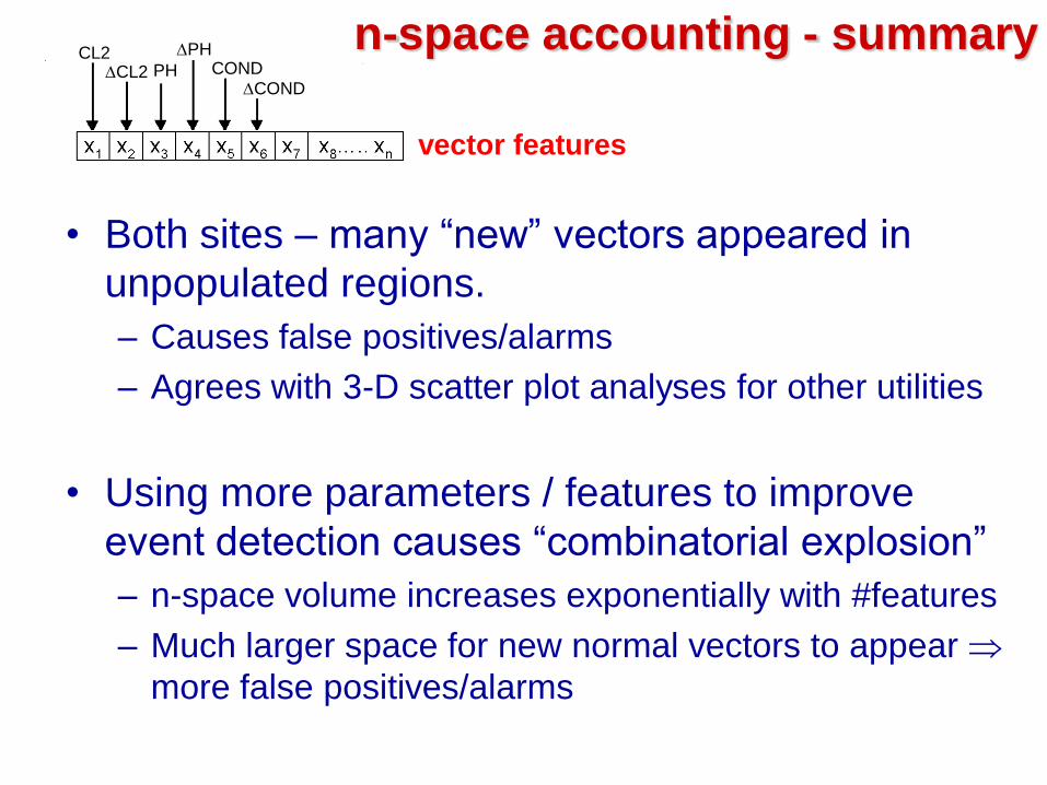
n-space accounting - summary
• Both sites – many “new” vectors appeared in
unpopulated regions.
– Causes false positives/alarms
– Agrees with 3-D scatter plot analyses for other utilities
• Using more parameters / features to improve
event detection causes “combinatorial explosion”
– n-space volume increases exponentially with #features
– Much larger space for new normal vectors to appear
more false positives/alarms
PH
DCOND
COND DCL2
CL2 DPH
vector features
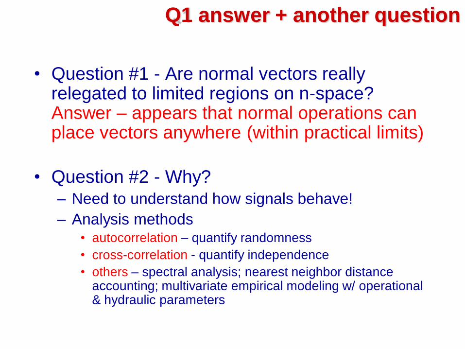
Q1 answer + another question
• Question #1 - Are normal vectors really relegated to limited regions on n-space? Answer – appears that normal operations can place vectors anywhere (within practical limits)
• Question #2 - Why? – Need to understand how signals behave!
– Analysis methods • autocorrelation – quantify randomness
• cross-correlation - quantify independence
• others – spectral analysis; nearest neighbor distance accounting; multivariate empirical modeling w/ operational & hydraulic parameters
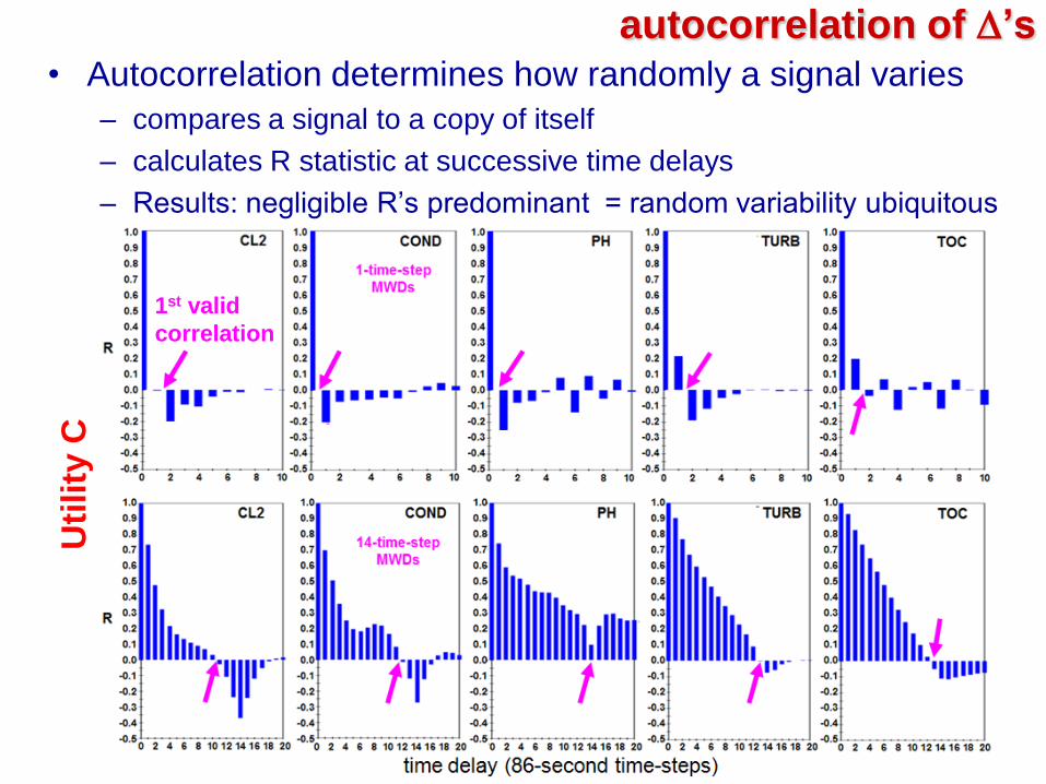
autocorrelation of D’s
• Autocorrelation determines how randomly a signal varies
– compares a signal to a copy of itself
– calculates R statistic at successive time delays
– Results: negligible R’s predominant = random variability ubiquitous
Uti
lity
C
1st valid
correlation
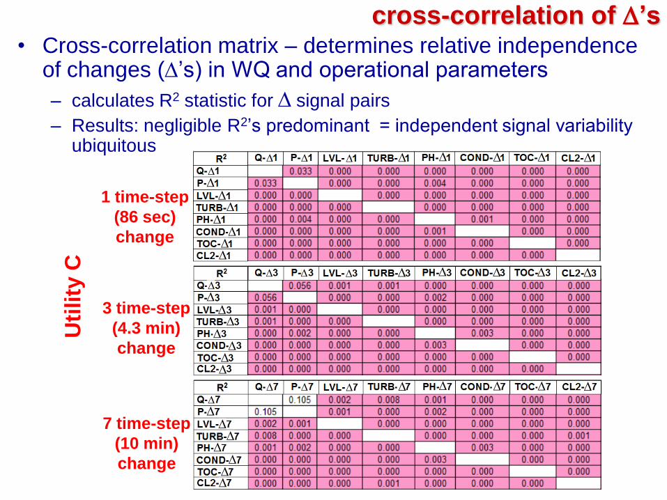
cross-correlation of D’s • Cross-correlation matrix – determines relative independence
of changes (D’s) in WQ and operational parameters
– calculates R2 statistic for D signal pairs
– Results: negligible R2’s predominant = independent signal variability ubiquitous
1 time-step
(86 sec)
change
3 time-step
(4.3 min)
change
7 time-step
(10 min)
change
Uti
lity
C
D D
D D
D D D D D D
D D
D D
D D
D D D D D D D D
D D D D D D D D
D D
D D
D D
D D
D D
D D
D D D
D
Q2 answer
• Question #1 - Are normal vectors really relegated to limited regions on n-space? Answer – appears that normal operations can place vectors anywhere
• Question #2 - Why? Answer – on a time scale 20
min, WQ signals vary with “apparent” randomness – random – because WQ trends are frequently interrupted
• random upstream mixing of waters having very different WQ’s
• randomly fluctuating flows, some propagated from afar
– “apparent” – because variability is due to “Laws of Physics”, but causes are unknown / unaccounted for by single-site approach
– conventional “lab chemistry” suppressed by ongoing mixing
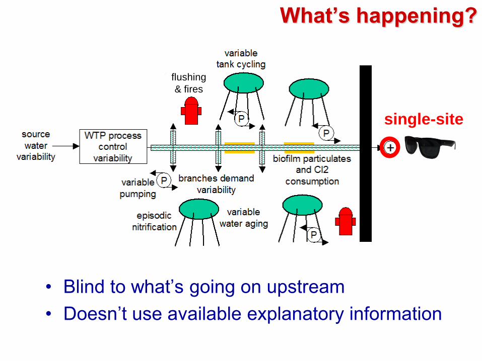
• Blind to what’s going on upstream
• Doesn’t use available explanatory information
flushing
& fires
single-site
What’s happening?
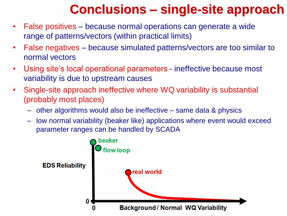
Conclusions – single-site approach
• False positives – because normal operations can generate a wide
range of patterns/vectors (within practical limits)
• False negatives – because simulated patterns/vectors are too similar to
normal vectors
• Using site’s local operational parameters - ineffective because most
variability is due to upstream causes
• Single-site approach ineffective where WQ variability is substantial
(probably most places)
– other algorithms would also be ineffective – same data & physics
– low normal variability (beaker like) applications where event would exceed
parameter ranges can be handled by SCADA

Multi-Site
Approach
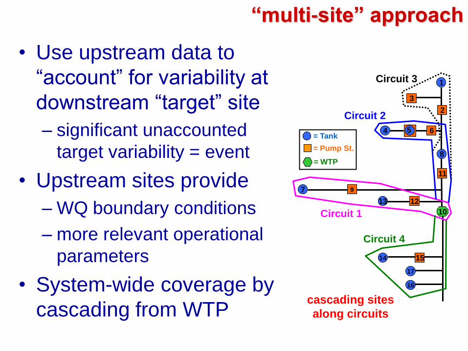
“multi-site” approach
• Use upstream data to
“account” for variability at
downstream “target” site
– significant unaccounted
target variability = event
• Upstream sites provide
– WQ boundary conditions
– more relevant operational
parameters
• System-wide coverage by
cascading from WTP
= Tank
= Pump St.
= WTP
17
7
14
1
9
2
5
8
3
16
15
11
6 4
13 12
Circuit 3
Circuit 1
Circuit 2
Circuit 4
10
cascading sites
along circuits
COND (mS/cm) TEMP (deg. F)
1-hour time steps (220 days, August to March)
CL2 (mg/l)
PH
CL2
PH
COND
TEMP
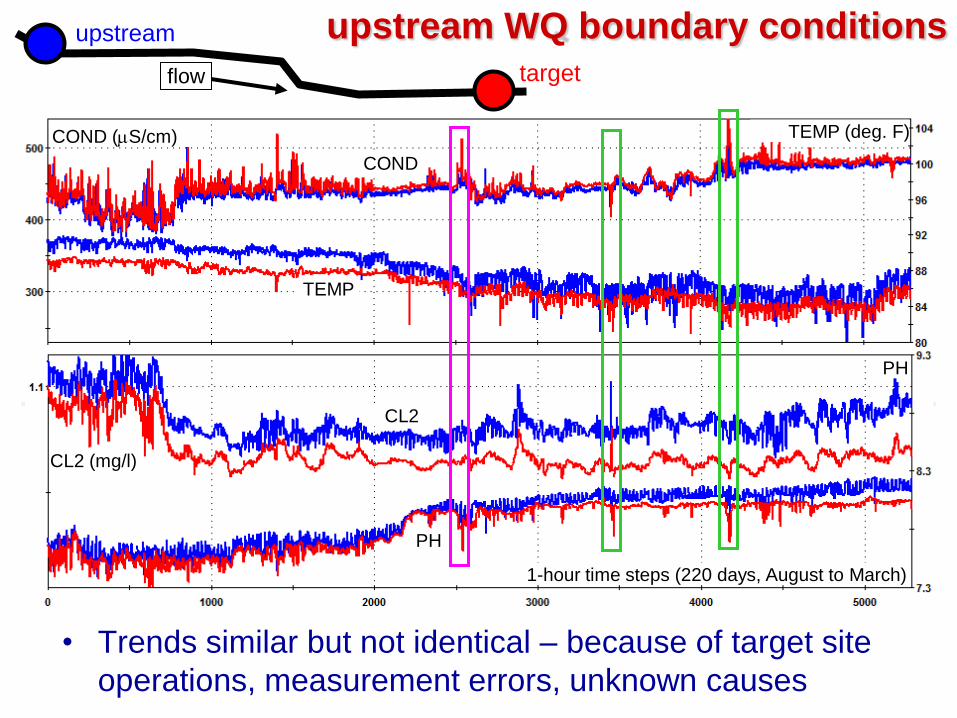
upstream WQ boundary conditions
• Trends similar but not identical – because of target site
operations, measurement errors, unknown causes
upstream
flow target
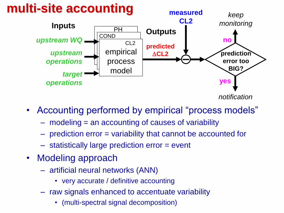
multi-site accounting
• Accounting performed by empirical “process models”
– modeling = an accounting of causes of variability
– prediction error = variability that cannot be accounted for
– statistically large prediction error = event
• Modeling approach
– artificial neural networks (ANN)
• very accurate / definitive accounting
– raw signals enhanced to accentuate variability
• (multi-spectral signal decomposition)
Inputs
predicted
DCL2
PH
measured
CL2
yes
keep
monitoring
COND
empirical
process
model
CL2 upstream WQ
upstream
operations
target
operations
Outputs
prediction
error too
BIG?
no
notification
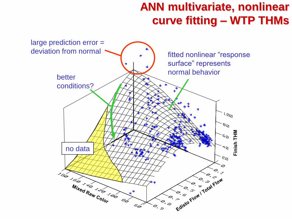
ANN multivariate, nonlinear
curve fitting – WTP THMs
no data
fitted nonlinear “response
surface” represents
normal behavior
large prediction error =
deviation from normal
better
conditions?
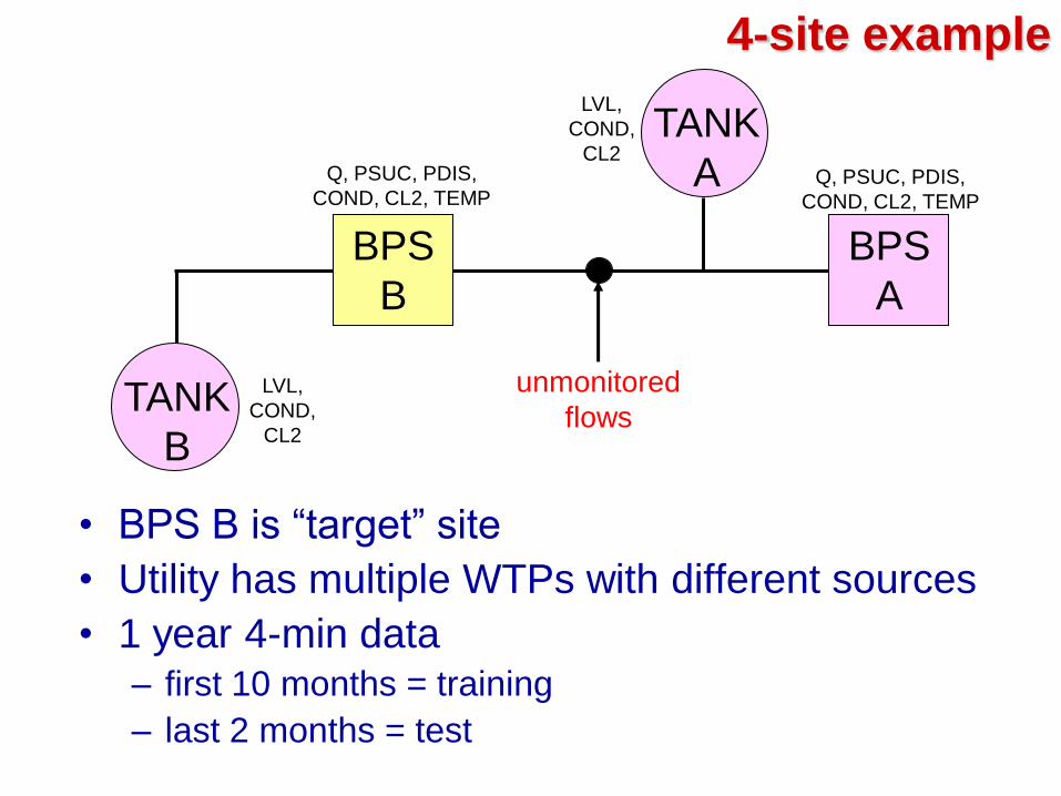
4-site example
• BPS B is “target” site
• Utility has multiple WTPs with different sources
• 1 year 4-min data – first 10 months = training
– last 2 months = test
BPS
A
TANK
A
unmonitored
flows
Q, PSUC, PDIS,
COND, CL2, TEMP
LVL,
COND,
CL2
TANK
B
BPS
B
Q, PSUC, PDIS,
COND, CL2, TEMP
LVL,
COND,
CL2
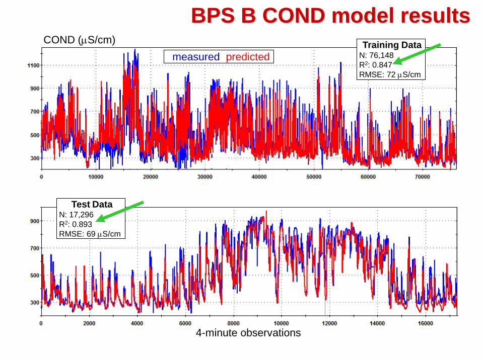
BPS B COND model results
4-minute observations
measured predicted
COND (mS/cm) Training Data
N: 76,148
R2: 0.847
RMSE: 72 mS/cm
Test Data N: 17,296
R2: 0.893
RMSE: 69 mS/cm

BPS B CL2 Process Model – training data CL2 (mg/l)
4-minute observations
measured predicted
Test Data N: 11,715
R2: 0.912
RMSE: 0.085 mg/l
Training Data N: 41,894
R2: 0.837
RMSE: 0.085 mg/l nitrification?
drop outs?
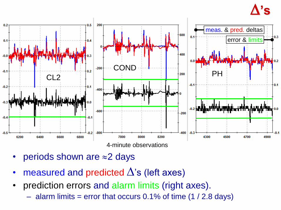
D’s
• periods shown are 2 days
• measured and predicted D’s (left axes)
• prediction errors and alarm limits (right axes). – alarm limits = error that occurs 0.1% of time (1 / 2.8 days)
CL2
COND PH
error & limits
meas. & pred. deltas
4-minute observations

ARMADA
Experimental
Multi-Site EDS
ARMADA testbed
• Experimental
• Does both single-site “nearest
neighbor” and multi-site event
detection
• Advanced data visualization for
monitoring processes
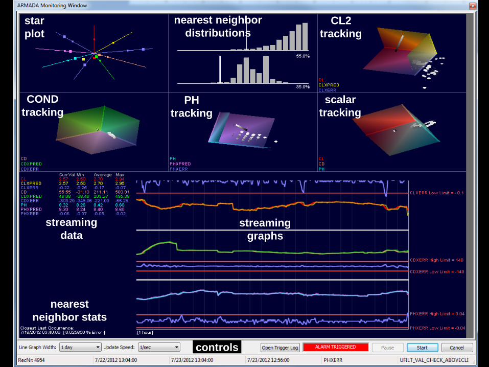
controls
streaming
data
star
plot
streaming
graphs
nearest
neighbor stats
COND
tracking PH
tracking
CL2
tracking
scalar
tracking
nearest neighbor
distributions
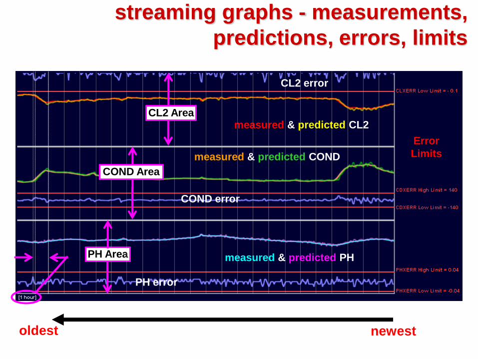
streaming graphs - measurements,
predictions, errors, limits
PH Area
CL2 error
measured & predicted CL2
Error
Limits
COND error
CL2 Area
COND Area
PH error
measured & predicted PH
measured & predicted COND
newest oldest
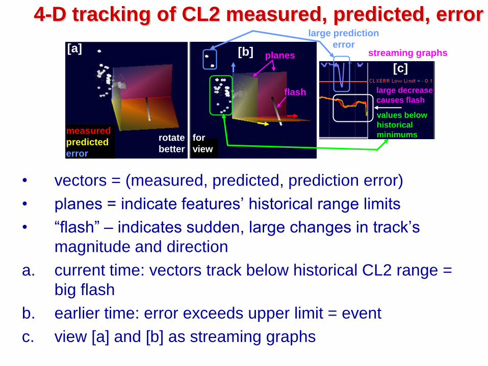
4-D tracking of CL2 measured, predicted, error
• vectors = (measured, predicted, prediction error)
• planes = indicate features’ historical range limits
• “flash” – indicates sudden, large changes in track’s
magnitude and direction
a. current time: vectors track below historical CL2 range =
big flash
b. earlier time: error exceeds upper limit = event
c. view [a] and [b] as streaming graphs
planes
large decrease
causes flash
large prediction
error
values below
historical
minimums
[a] [b]
[c]
flash
streaming graphs
measured
predicted
error
rotate for
better view
Conclusions – multi-site approach
• Potential big improvement over single-site – understands each site’s process physics
– uses known causes of WQ variability to reduce false positives & negatives
– cases indicate 80-90%+ of target WQ variability can be accounted for
• In research phase - ARMADA “demo” available
• Multi-site’s process models – predict cause-effect – can also use to control WQ in distribution system
• Other reasons to monitor distribution system – control processes to improve WQ at points of delivery
– detect common problems - low CL2, nitrification, line integrity, DBPs

Series of Tanks and Pump Stations – Util. A
• CL2 decreases downstream and in tanks
CL2 (
mg/l)
1-minute time steps 1/1/05 – 11/16/09
Pump-A
Tank-A
Pump-B
Tank-B
9 months

Thanks for your
attention!
Ed Roehl or John Cook
Advanced Data Mining Intl
864.201.8679
This slide shows the difference between
test results and reality
Recommended