Wireless Sensor Network (CSE 6812)
Dr. Mahmuda Naznin
Department of Computer Science Engineering
Date: May 10, 2015

Grading Policy
15%-Presentation
15%-Critic writing/Survey
30%-Mid Term Exam
40%-Final Exam

Challenges and Issues Deployment Coverage and Connectivity Tracking Sensing and Transmission Routing Minimizing Range of Communication Faster Routing, switching How to communicate with standard internet protocols Sensor database Data aggregation and transmission Query processing Security issues

4
Introduction to WSN

5
Background Sensors
Enabled by recent advances in MEMS technology
Integrated Wireless Transceiver
Limited in Energy Computation Storage Transmission range Bandwidth
Battery
Memory
CPU
Sensing Hardware
Wireless Transceiver

6
Background
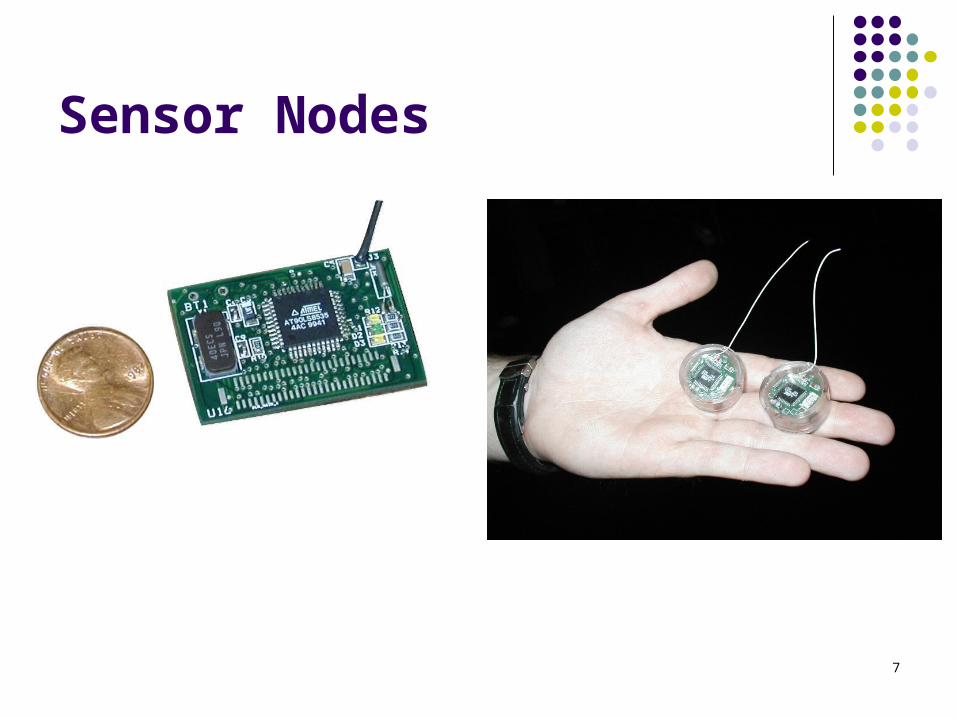
7
Sensor Nodes

8
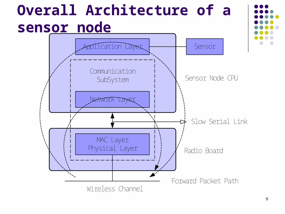
Sensors (contd.) The overall architecture of a sensor
node consists of: The sensor node processing
subsystem running on sensor node main CPU
The sensor subsystem and The communication subsystem
The processor and radio board includes: TI MSP430 microcontroller with
10kB RAM 16-bit RISC with 48K Program
Flash IEEE 802.15.4 compliant radio
at 250 Mbps 1MB external data flash Runs TinyOS 1.1.10 or higher Two AA batteries or USB 1.8 mA (active); 5.1uA (sleep)
Crossbow MoteTPR2400CA-TelosB
9
Overall Architecture of a sensor node
Appl i cati on Layer
Network Layer
MAC LayerPhysi cal Layer
Communi cati onSubSystem
Wi rel ess Channel
Sl ow Seri al Li nk
Sensor
Sensor Node CPU
Radi o Board
Forward Packet Path

10
Wireless Sensor Networks collection of networked sensors
11
Networked vs. individual sensors Extended range of sensing:
Cover a wider area of operation Redundancy:
Multiple nodes close to each other increase fault tolerance
Improved accuracy: Sensor nodes collaborate and combine their data
to increase the accuracy of sensed data Extended functionality:
Sensor nodes can not only perform sensing functionality, but also provide forwarding service.
12
Applications of sensor networks
Physical security for military operations Indoor/Outdoor Environmental monitoring Seismic and structural monitoring Industrial automation Bio-medical applications Health and Wellness Monitoring Inventory Location Awareness Future consumer applications, including
smart homes.
13
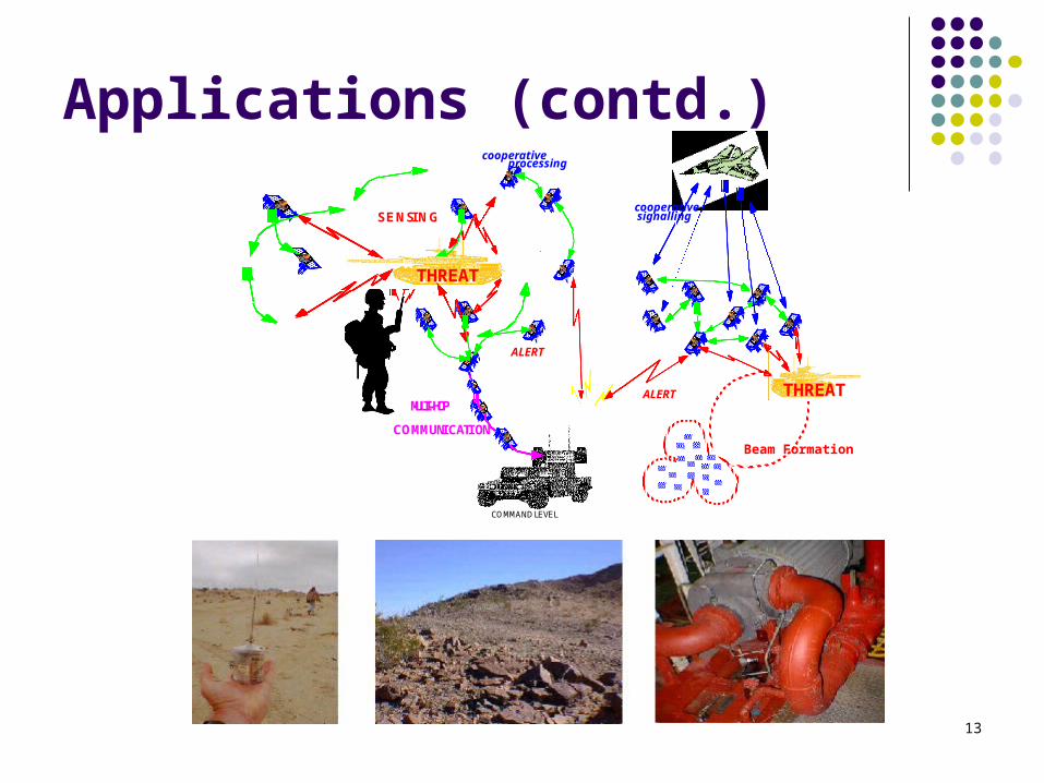
Applications (contd.)
ALERT
Beam Formation
cooperative
ALERT
COMMAND LEVEL
SENSING
COMMUNICATION
THREAT
processing
MULTI-HOP
cooperativesignalling
THREAT
14
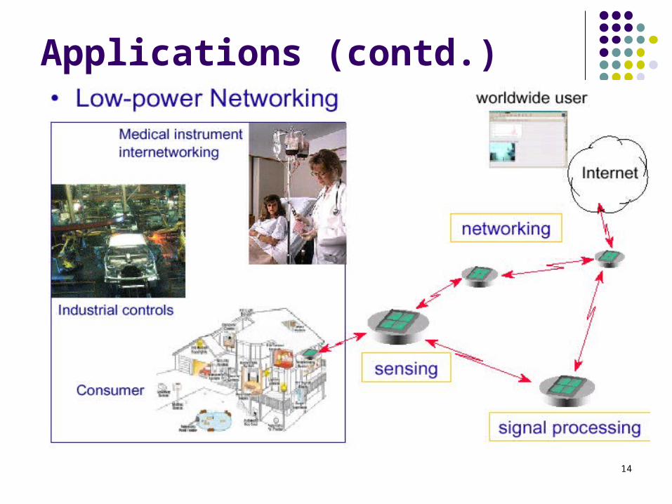
Applications (contd.)
15
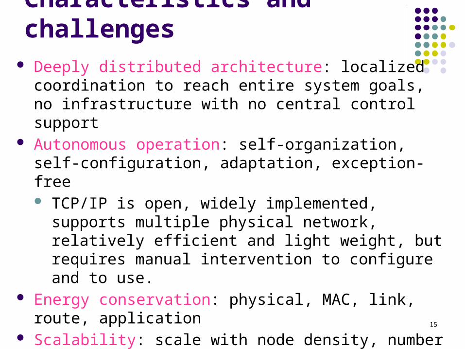
Characteristics and challenges Deeply distributed architecture: localized coordination to
reach entire system goals, no infrastructure with no central control support
Autonomous operation: self-organization, self-configuration, adaptation, exception-free TCP/IP is open, widely implemented, supports multiple
physical network, relatively efficient and light weight, but requires manual intervention to configure and to use.
Energy conservation: physical, MAC, link, route, application Scalability: scale with node density, number and kinds of
networks Data centric network: address free route, named data,
reinforcement-based adaptation, in-network data aggregation

16
Challenges (contd. ) Challenges
Limited battery power Limited storage and computation Lower bandwidth and high error rates Scalability to 1000s of nodes
Network Protocol Design Goals Operate in self-configured mode (no infrastructure
network support) Limit memory footprint of protocols Limit computation needs of protocols -> simple,
yet efficient protocols Conserve battery power in all ways possible

17
Why not Traditional Network Protocols? Traditional networks require significant
amount of routing data storage and computation Sensor nodes are limited in memory and CPU
Topology changes due to node mobility are infrequent as in most applications sensor nodes are stationary Topology changes when nodes die in the network
due to energy dissipation Scalability with several hundred to a few
thousand nodes not well established
18
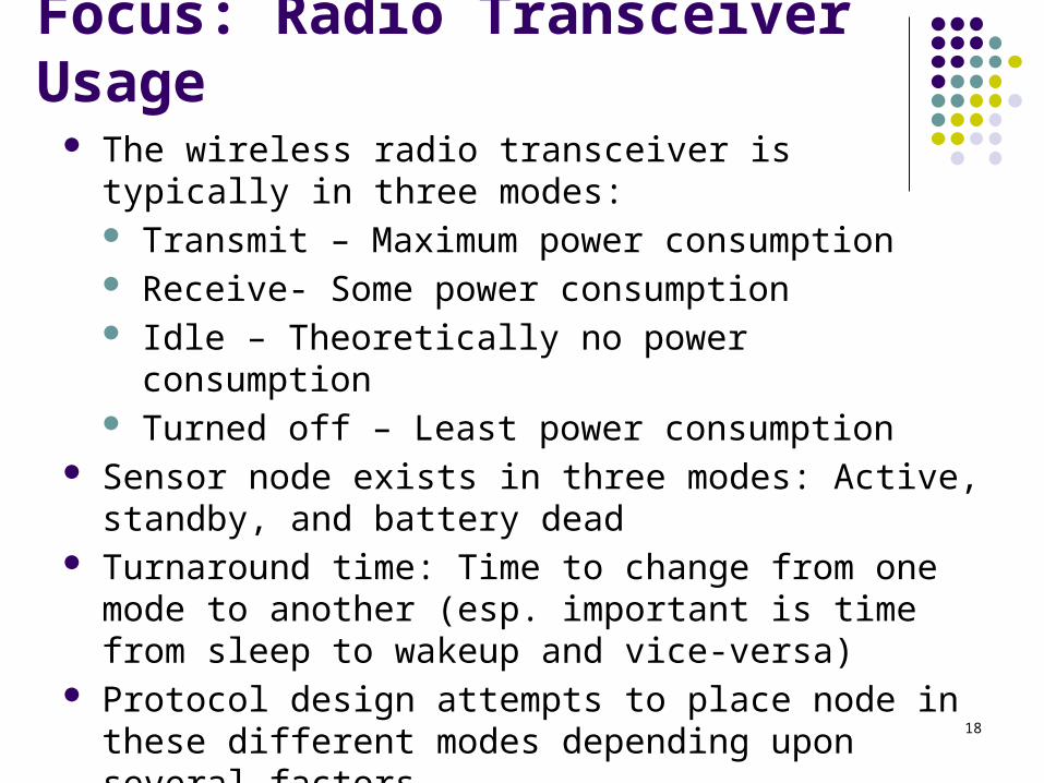
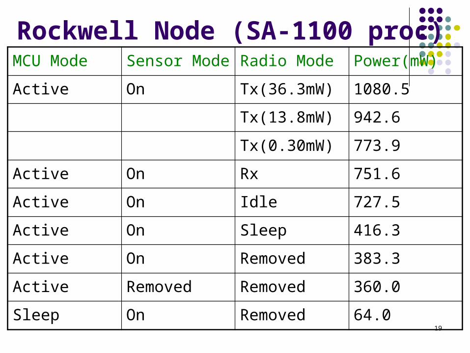
Focus: Radio Transceiver Usage The wireless radio transceiver is typically in three
modes: Transmit – Maximum power consumption Receive- Some power consumption Idle – Theoretically no power consumption Turned off – Least power consumption
Sensor node exists in three modes: Active, standby, and battery dead
Turnaround time: Time to change from one mode to another (esp. important is time from sleep to wakeup and vice-versa)
Protocol design attempts to place node in these different modes depending upon several factors
19
Rockwell Node (SA-1100 proc)MCU Mode Sensor Mode Radio Mode Power(mW)
Active On Tx(36.3mW) 1080.5
Tx(13.8mW) 942.6
Tx(0.30mW) 773.9
Active On Rx 751.6
Active On Idle 727.5
Active On Sleep 416.3
Active On Removed 383.3
Active Removed Removed 360.0
Sleep On Removed 64.0

20
UCLA Medusa node (ATMEL CPU)MCU Mode Sensor Radio(mW) Data rate Power(mW)
Active On Tx(0.74,OOK) 2.4Kbps 24.58
Tx(0.74,OOK) 19.2Kbps 25.37
Tx(0.10,OOK) 2.4Kbps 19.24
Tx(0.74,OOK) 19.2Kbps 20.05
Tx(0.74,ASK) 19.2Kbps 27.46
Tx(0.10,ASK) 2.4Kbps 21.26
Active On Rx - 22.20
Active On Idle - 22.06
Active On Off - 9.72
Idle On Off - 5.92
Sleep Off Off - 0.02

21
Energy conservationPhysical layer
• Low power circuit(CMOS, ASIC) design
• Optimum hardware/software function division
• Energy effective waveform/code design
• Adaptive RF power control
MAC sub-layer • Energy effective MAC protocol
• Collision free, reduce retransmission and transceiver on-times
• Intermittent, synchronized operation
• Rendezvous protocols
Link layer
Network layer
Application layer
• FEC versus ARQ schemes; Link packet length adapt.
• Multi-hop route determination
• Energy aware route algorithm
• Route cache, directed diffusion
• Video applications: compression and frame-dropping
• In-network data aggregation and fusion
See Jones, Sivalingam, Agrawal, and Chen survey article in ACM WINET, July 2001;See Lindsey, Sivalingam, and Raghavendra book chapter in Wiley Handbook of Mobile Computing, Ivan Stojmenovic, Editor, 2002.

22
Coverage, Exposure and Deployment
23
Coverage Problems
Coverage: is a measure of the Quality of service of a sensor network
How well can the network observe (or cover) a given event? For example, intruder detection; animal or fire
detection Coverage depends upon:
Range and sensitivity of sensing nodes Location and density of sensing nodes in given
region

24
Coverage, contd.
Worst-Case Coverage: Areas of breach (lowest coverage) Can be used to determine if additional sensors
needed Best-Case Coverage: Areas of best coverage
Can be used by a friendly user to navigate in those areas

25
Coverage, contd. Given: A field A with sensors S, where for each sensor $s_i
its location (x, y) is known (How? Based on the Localization Techniques described earlier). Areas I and F are initial and final locations of an agent traversing the field.
Problem: Identify the maximal breach path in S, starting in I and ending in F P is defined as the locus of points p in the region, where p
is in P if the distance from p to the closest sensor is maximized.
I and F are arbitrarily specified inputs. Solution: Determine the Voronoi diagram corresponding to
the sensor graph. The path P will be composed of line segments that belong to the Voronoi diagram.
26
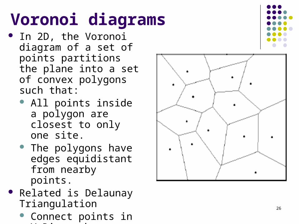
Voronoi diagrams In 2D, the Voronoi diagram
of a set of points partitions the plane into a set of convex polygons such that: All points inside a
polygon are closest to only one site.
The polygons have edges equidistant from nearby points.
Related is Delaunay Triangulation Connect points in V-Diag.
whose polygons share a common edge.

27
Worst-Case Coverage: Alg.
1. Generate the bounded Voronoi diagrama. Let U and L denote vertex set and links of diag.
2. Create a graph with vertices from set U and links from L
a. Weight of link in graph = minimum distance from all sensors in S
3. Do a breadth-first search to determine a path from I to F in the graph, such that the path has maximum edge cost
4. Multiple such paths possible

28
Best-Case Coverage
Problem: Identify P_S, the path with maximum support in S, starting at I and ending in F.
Solution: Use Delaunay triangulation The best path will be one connecting some of the
sensor nodes Similar approach to Max. Breach Path
Use Delaunay instead of Voronoi The edge cost in the graph G, will be the length of
the Delaunay triangle line segment.

DAWN Lab / UMBC 29
Examples
Fig. on left shows the bounded Voronoi diagram and the maximal breach path
Fig. on right shows the Delaunay Triangulation and the maximal support path
Question: Once these are determined, how to use these?

30
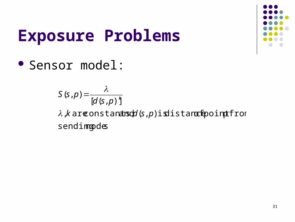
Exposure Problems
Exposure is related to the coverage Exposure may be defined as the expected
ability of observing a target in the sensor field Formally defined as the integral of the
sensing function (depends on distance from sensors) on a path from P_s to P_d
Sensing function depends on nature of sensors
31
Exposure Problems
Sensor model:
s node sending
from ppoint of distance is ),( and constants; are ,
)],([),(
psdk
psdpsS
k

32
Exposure at a point
All-Sensor Field Intensity at Point p in field with n sensors denoted by
Closest-Sensor Field Intensity at Point p:
),(),(1
psSpFIn
iiA
},...,,{ 21 nsss
),(),(
),(),(|
min
min
pSSpFI
SspsdpsdSsS
C
iimm

33
Exposure along a path Suppose object O is traveling from point p(t1)
to p(t2) along path p(t). Exposure for object O during interval t1 to t2
along p(t) is defined as:
22
)or (21
)()()(
then y(t))(x(t), p(t) If
length arc ofelement theis )(
)())(,(],),([
2
1
dt
tdy
dt
tdx
dt
tdp
dt
tdp
dtdt
tdptpFItttpE
t
t
CA

34
Exposure: Properties
Consider only 1 sensor at location (0,0). Let
Determine the path from a=(1,0) to point b=(X,Y) with minimum exposure Determine x(t), y(t) such that x(0) = 1; y(0) = 0;
x(1) = X; y(1) = Y and the exposure function is minimized.
22),(1 1
)],(),0,0([yx
yxpsS psd
2E and
2sin,
2cos
tt

DAWN Lab / UMBC 35
Exposure: Properties Given a sensor s and two points a and b, such d(s,a)=d(s,b),
then the minimum exposure path between a and b is that part of the circle centered as s and passing through a and b.
Theorem: Let the sensor be located at (0,0) in a unit field. The minimum exposure path from (1,-1) to (-1,1) is as below:
S=(0,0)

DAWN Lab / UMBC 36
Exposure: Properties Let s be a sensor in a polygonal field with
vertices v1,…,vn. For the inscribed circle of the polygon, let
edge v_i,v_{i+1} be tangent at point u_i The minimum exposure path from vertex v_i
to vertex v_j consists of: Line segment from v_i to u_i Part of inscribed circle from u_i to u_j Line segment from u_j to v_j (OR) in the opposite direction (from v_i to u_j etc)
Problem of MEP between 2 points in same corner or between 2 points inside the inscribed circle is open
DAWN Lab / UMBC 37
Generic Exposure Problem
Given a network with randomly placed sensor nodes, how to determine minimum exp. Path
Solution: Tessellate the network into a set of equidistant
grid points (with varying degree of precision) For each edge in the grid network, assign an
edge equal to the exposure along the edge (integrated from the sensor function)
Using Dijkstra’s algorithm, determine the shortest path from a source (based on edge weights)
This is the min. exposure path
Recommended