Wind Driven Circulation I:Planetary boundary Layer
near the sea surface

Monin-Obukhoff Similarity TheorySurface layer (several tens of meters above surface, 10-15% of
the planetary boundary layer) in nearly steady condition 1. Vertical turbulent flux is nearly constant2. horizontal homogeneity (the scale of vertical variation is
much smaller than horizontal) 3. The turbulent mixing length l=z
=0.4±0.01 is von Karman constantMomentum flux
() is a universal function of€ ς=zL
L is the Monin-Obukhoff length€ zu*∂u∂z=φς() € τ=′ u ′ w =ρu*2
u* is frictional velocity
At altitudes below L, shear production of turbulent kinetic energy
dominates over buoyant production of turbulence. € L=−Tvu*3gκ′ w ′ T v

In neutral condition, ()=1
€ ∂u∂z=u*κz
von Karman logarithmic law of wall
€ u=u*κlnzzo
€ τ=ρu*2=ρκ2lnzzou2The surface momentum flux is
If we choose wind measurement at a certain height, e.g., 10m above the sea surface, the bulk formula is
€ τ=ρC10Du102€
C10D=κ2lnz10zois 10m neutral drag coefficient
zo is aerodynamic roughness length

Surface wind stress• Approaching sea surface, the geostrophic
balance is broken, even for large scales. • The major reason is the influences of the winds
blowing over the sea surface, which causes the transfer of momentum (and energy) into the ocean through turbulent processes.
• The surface momentum flux into ocean is called the surface wind stress ( ), which is the tangential force (in the direction of the wind) exerting on the ocean per unit area (Unit: Newton per square meter)
• The wind stress effect can be constructed as a boundary condition to the equation of motion as
τr
τρ rr
==
∂∂
0zz
VA Hz

Wind stress Calculation• Direct measurement of wind stress is difficult.• Wind stress is mostly derived from meteorological
observations near the sea surface using the bulk formula with empirical parameters.
• The bulk formula for wind stress has the form
VVC ad
rr ρτ =
aρWhere is air density (about 1.2 kg/m3 at mid-latitudes), V (m/s), the wind speed at 10 meters above the sea surface, Cd, the empirical determined drag coefficient
Drag Coefficient Cd
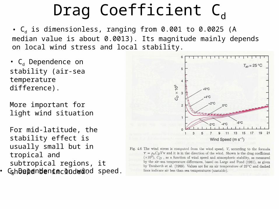
• Cd is dimensionless, ranging from 0.001 to 0.0025 (A median value is about 0.0013). Its magnitude mainly depends on local wind stress and local stability.
• Cd Dependence on wind speed.
• Cd Dependence on stability (air-sea temperature difference).
More important for light wind situation For mid-latitude, the stability effect is usually small but in tropical and subtropical regions, it should be included.

Cd dependence on wind speed in neutral
condition
Large uncertainty between estimates(especially in low wind speed).
Lack data in high wind

Annual Mean surface wind stress
Unit: N/m2, from Surface Marine Data (NODC)

December-January-February mean wind stress
Unit: N/m2, from Surface Marine Data (NODC)

December-January-February mean wind stress
Unit: N/m2, from Scatterometer data from ERS1 and 2

June-July-August mean wind stress
Unit: N/m2, from Surface Marine Data (NODC)

Unit: N/m2, Scatterometers from ERS1 and 2
June-July-August mean wind stress

The primitive equation
gzp ρ−=∂∂
xuAxxx ∂∂=ρτ y
uAyxy ∂∂=ρτ
2
2
2
2
2
21zuA
yuA
xuAfv
xp
zuw
yuv
xuu
tu
zyx ∂∂+∂
∂+∂∂++∂
∂−=∂∂+∂
∂+∂∂+∂
∂ρ
2
2
2
2
2
21zvA
yvA
xvAfu
yp
zvw
yvv
xvu
tv
zyx ∂∂+∂
∂+∂∂+−∂
∂−=∂∂+∂
∂+∂∂+∂
∂ρ
0=∂∂+∂
∂+∂∂
zw
yv
xu
Since the turbulent momentum transports are
(1)
(2)
(3)
(4)
zuAzxz ∂∂=ρτ, , etc
⎟⎟⎠
⎞⎜⎜⎝
⎛
∂∂
+∂
∂+
∂∂
++∂∂
−=∂∂
+∂∂
+∂∂
+∂∂
yyxfv
x
p
z
uw
y
uv
x
uu
t
u xzxyxx τττ
ρρ
11
⎟⎟⎠
⎞⎜⎜⎝
⎛
∂
∂+
∂
∂+
∂
∂+−
∂∂
−=∂∂
+∂∂
+∂∂
+∂∂
yyxfu
y
p
z
vw
y
vv
x
vu
t
v yzyyyx τττ
ρρ
11
We can also write the momentum equations in more general forms
zuAzxz ∂∂=ρτ 0
zvAzyz ∂∂=ρτ 0At the sea surface (z=0),
turbulent transport is wind stress. ,

Assumption for the Ekman layer near the surface
• Az=const• Steady state (steady wind forcing for long time)• Small Rossby number
• Large vertical Ekman Number
• Homogeneous water (ρ=const)• f-plane (f=const)• no lateral boundaries (1-d problem)• infinitely deep water below the sea surface
€ Ro=Ou∂u∂x ⎛ ⎝ ⎜ ⎞ ⎠ ⎟Ofv()=U2LfoU=UfoL<<1€
Ez=OAz∂2u∂z2 ⎛ ⎝ ⎜ ⎞ ⎠ ⎟Ofv()=AzUH2foU=AzfoH2

Ekman layer
• Near the surface, there is a three-way force balance
Coriolis force+vertical dissipation+pressure gradient force=0
011 =∂∂−
∂∂+
xp
zfv x
ρτ
ρ
011 =∂∂−
∂∂+−
yp
zfu y
ρτ
ρ
zuAzx ∂∂=ρτ
Take
zvAzy ∂∂=ρτ
and let
(note that VE is not small in comparison to Vg in this region)
02
2
2
2
≈∂∂
−=∂∂
+zu
AzuAfv g
zE
zE
02
2
2
2
≈∂∂
−=∂∂− +
zv
AzvAfu g
zE
zE
then € u,v()=ug,vg()+uE,vE()Geostrophic current
Ageostrophic (Ekman) current

The Ekman problem0
2
2
=∂∂
+zuAfv E
zE
02
2
=∂∂− +
zvAfu E
zE
Boundary conditionsAt z=0,
xE
z zuA τρ =∂∂
yE
z zvA τρ =∂∂
As z -0→Eu,
.0→Ev
Let EEE ivuV += (complex variable), take (1) + i(2), we have
02
2=−
∂∂
EE
z ifVzVA
,.
(1)
(2)
(3)
(4)
(5)
(6)
€ fvE+Az∂2uE∂z2+i−fuE+Az∂2vE∂z2 ⎛ ⎝ ⎜ ⎞ ⎠ ⎟=0€
Az∂2uE+ivE( )∂z2−ifuE−vEi ⎛ ⎝ ⎜ ⎞ ⎠ ⎟=0€ i2=i⋅i=−1Since
€ i=−1i
€ Az∂2uE+ivE( )∂z2−ifuE+ivE( )=0 (7)

z=0,x
Ez z
uA τρ =∂∂
yE
z zvA τρ =∂∂
As z - ,0→Eu
0→Ev
Group equations (7), (8), and (9) together, we have
At z=0,
As z - 0→EV
(3)
(4)
(5)
(6)
Take (3) + i (4), we have
€ ρAz∂uE+ivE( )∂z=τx+iτy
€ τ=τx+iτyDefine
€ ρAz∂VE∂z=τ
Take (5) + i (6), we have
€ uE+ivE=VE→0(8)
(9)
€ ∂2VE∂z2−ifAzVE=0€ ∂VE∂z=τρAz (7)
(8)
(9)

Assume the solution for (7) has the following form
€ ∂2VE∂z2−ifAzVE=0€ VE=eαzTake into
€ α2eαz−ifAzeαz=0We have
€ α2=ifAz
If f > 0,
€ i=eiπ2=eiπ4=cosπ4 ⎛ ⎝ ⎜ ⎞ ⎠ ⎟+isinπ4 ⎛ ⎝ ⎜ ⎞ ⎠ ⎟=12+i12=1+i2€ α=±ifAz=±1+i2fAz
If f < 0,
€ α=±ifAz=±1+i2−fAz=±1+i2ifAz=±1−i2fAz
In above derivations, we have used the following equality:
For f > 0, the general solution of (7) can be written as
⎟⎟⎟⎟
⎠
⎞
⎜⎜⎜⎜
⎝
⎛
⎟⎠⎞⎜
⎝⎛
⎟⎟⎟⎟
⎠
⎞
⎜⎜⎜⎜
⎝
⎛
⎟⎠⎞⎜
⎝⎛
⎟⎟⎟
⎠
⎞
⎜⎜⎜
⎝
⎛
⎟⎟⎟
⎠
⎞
⎜⎜⎜
⎝
⎛
+−++=−+= ziA
fBziA
fAzAifBz
AifAV
zzzz
E 12
exp12
expexpexp
⎟⎟⎟
⎠
⎞
⎜⎜⎜
⎝
⎛
⎟⎠⎞⎜
⎝⎛
⎟⎠⎞⎜
⎝⎛
+−
−= ziAf
fA
iV
zzE 1
2exp
2
1
ρ
τ
At z=0,
€ ∂VE∂z=τρAz
(8)As z - 0→EV
(9)
⎟⎟⎟⎟
⎠
⎞
⎜⎜⎜⎜
⎝
⎛
⎟⎠⎞⎜
⎝⎛
⎟⎟⎟⎟
⎠
⎞
⎜⎜⎜⎜
⎝
⎛
⎟⎠⎞⎜
⎝⎛
⎟⎟⎟
⎠
⎞
⎜⎜⎜
⎝
⎛
⎟⎟⎟
⎠
⎞
⎜⎜⎜
⎝
⎛
+−++=−+= ziA
fBziA
fAzAifBz
AifAV
zzzz
E 12
exp12
expexpexp
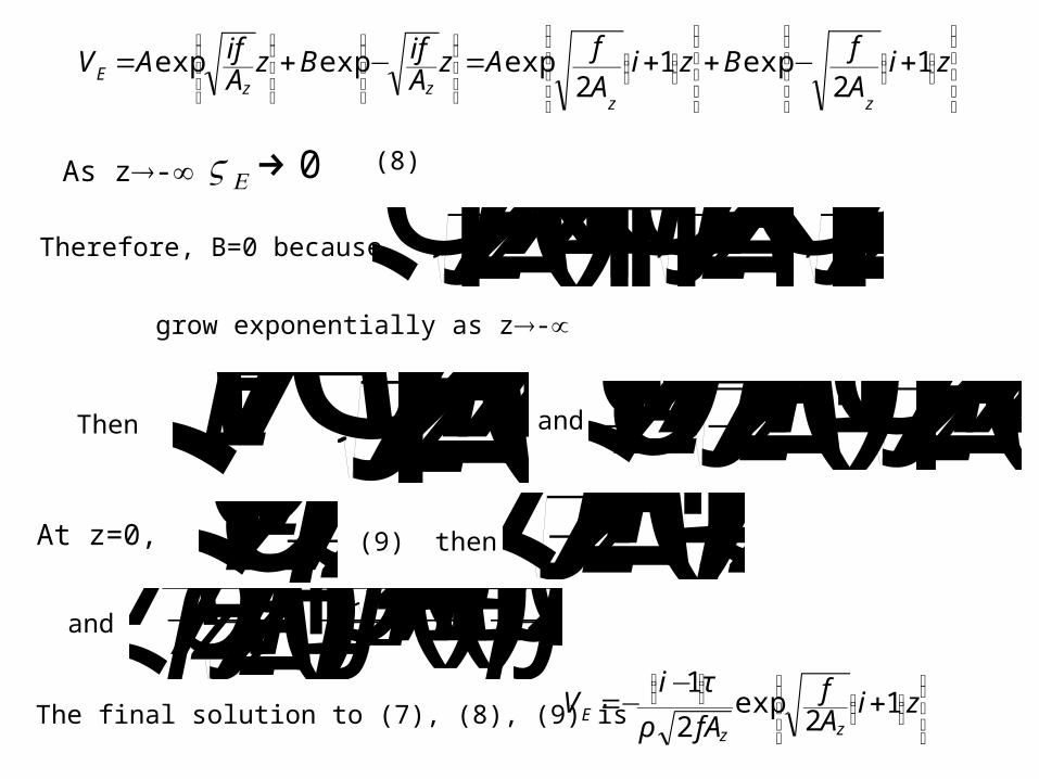
Therefore, B=0 because
€ exp−f2Azi+1()z ⎡ ⎣ ⎢ ⎤ ⎦ ⎥=exp−if2Azz ⎡ ⎣ ⎢ ⎤ ⎦ ⎥⋅exp−f2Azz ⎡ ⎣ ⎢ ⎤ ⎦ ⎥
grow exponentially as z-
€ VE=Aexpf2Azi+1()z ⎡ ⎣ ⎢ ⎤ ⎦ ⎥Then and
€ ∂VE∂z=Af2Azi+1()expf2Azi+1()z ⎡ ⎣ ⎢ ⎤ ⎦ ⎥
€ Af2Azi+1()=τρAzthen
€ A=τρAzf2Azi+1()=2τi−1()ρfAzi+1()i−1()=i−1()τρ2fAzand
The final solution to (7), (8), (9) is

Set , where Si
eφττ = and ⎟
⎟⎠
⎞⎜⎜⎝
⎛−=x
yS τ
τφ 1tan
⎟⎟⎟⎟
⎠
⎞
⎜⎜⎜⎜
⎝
⎛
−+= 42
2 πφ
ρτ Sz
zAfi
z
zzA
f
E efA
eV
Also note that iei 4
21 π−=−−
⎟⎟⎟
⎠
⎞
⎜⎜⎜
⎝
⎛
⎟⎠⎞⎜
⎝⎛
⎟⎠⎞⎜
⎝⎛
+−
−= ziAf
fA
iV
zzE 1
2exp
2
1
ρ
τGiven
€ τ=τx2+τy2We have
€ VE=τef2AzzρfAzCurrent Speed:
Phase (direction):€ φ=f2Azz+φS−π4(=0, eastward)

€ VE=τef2AzzρfAzeif2Azz+φS−π4 ⎛ ⎝ ⎜ ⎜ ⎞ ⎠ ⎟ ⎟=τef2AzzρfAzcosf2Azz+φS−π4 ⎛ ⎝ ⎜ ⎜ ⎞ ⎠ ⎟ ⎟+isinf2Azz+φS−π4 ⎛ ⎝ ⎜ ⎜ ⎞ ⎠ ⎟ ⎟ ⎡ ⎣ ⎢ ⎢ ⎤ ⎦ ⎥ ⎥
€ uE=τef2AzzρfAzcosf2Azz+φS−π4 ⎛ ⎝ ⎜ ⎜ ⎞ ⎠ ⎟ ⎟
€ vE=τef2AzzρfAzsinf2Azz+φS−π4 ⎛ ⎝ ⎜ ⎜ ⎞ ⎠ ⎟ ⎟€
uE=τef2AzzρfAzcos−f2Azz+φS+π4 ⎛ ⎝ ⎜ ⎜ ⎞ ⎠ ⎟ ⎟€
vE=τef2AzzρfAzsin−f2Azz+φS+π4 ⎛ ⎝ ⎜ ⎜ ⎞ ⎠ ⎟ ⎟If f < 0,
Recommended