What Makes a Patch Distinct?
CVPR2013 POSTER

Outline
IntroductionMethodResultsDiscussion
Most previous work assert that distinctness is the dominating factor.
Some focus on the patterns, others on the colors, and several add high-level cues and priors.
Introduction
Introduction
Our key idea is that the analysis of the inner statistics of patches in the image provides acute insight on the distinctness of regions.
use PCA to represent the set of patches of an image and use this representation to determine distinctness.
Introduction
Pattern Distinctness Color Distinctness Putting it all together
Method
Pattern Distinctness
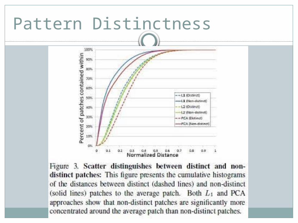
Our first observation is that the non-distinct patches of a natural image are mostly concentrated in the high-dimensional space, while distinct patches are more scattered.
Pattern Distinctness
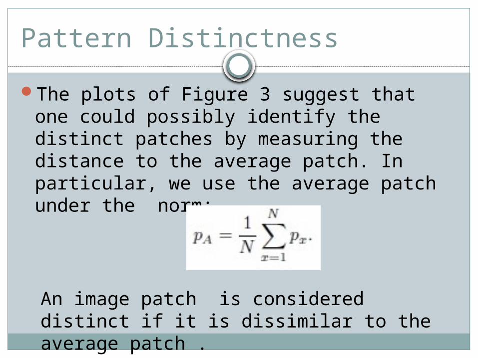
The plots of Figure 3 suggest that one could possibly identify the distinct patches by measuring the distance to the average patch. In particular, we use the average patch under the norm:
Pattern Distinctness
An image patch is considered distinct if it is dissimilar to the average patch .
Pattern Distinctness
Suppose that a certain patch appears in two different images.
These two images could have the same average patch, thus the distance of the patch to the average would be equal.
Pattern Distinctness
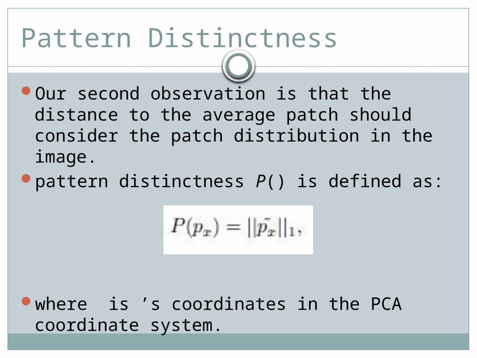
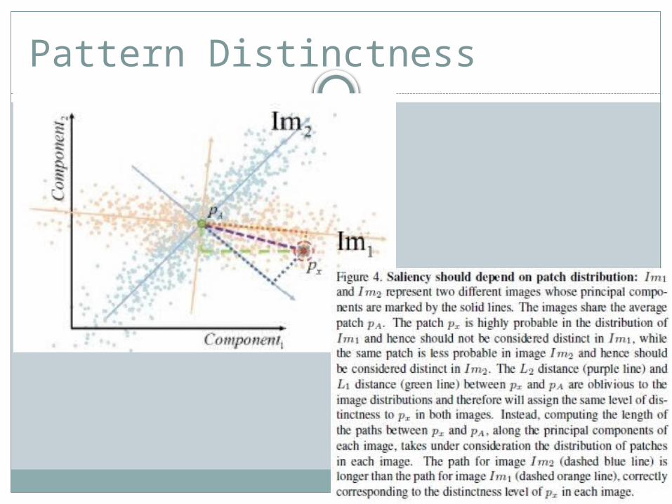
Our second observation is that the distance to the average patch should consider the patch distribution in the image.
pattern distinctness P() is defined as:
where is ’s coordinates in the PCA coordinate system.
Pattern Distinctness
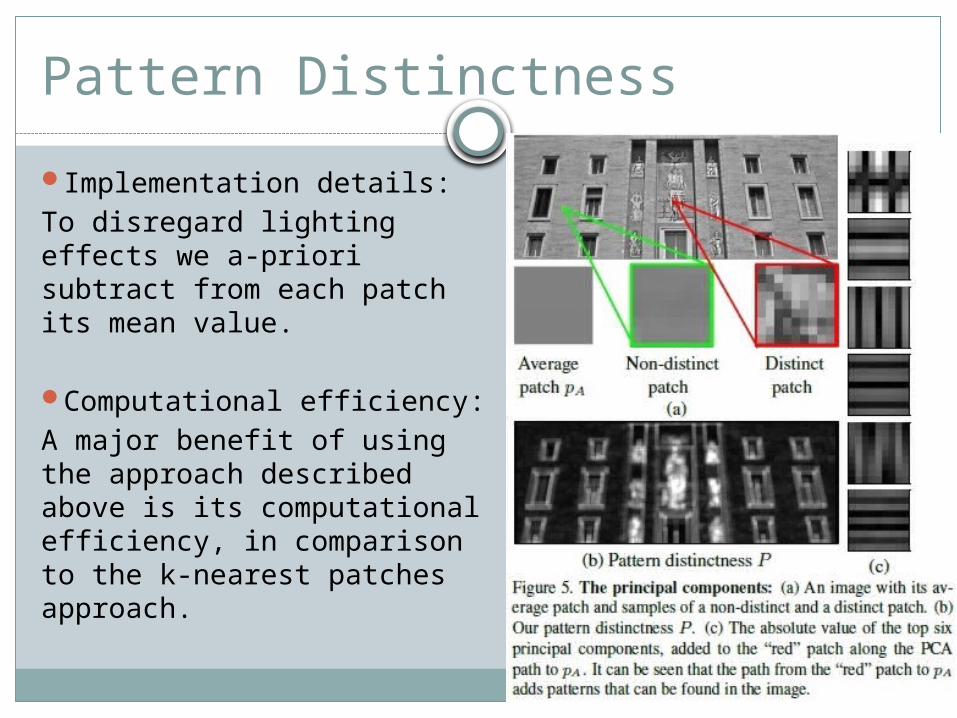
Implementation details:To disregard lighting effects we a-priori subtract from each patch its mean value.
Computational efficiency:A major benefit of using the approach described above is its computational efficiency, in comparison to the k-nearest patches approach.
Pattern Distinctness
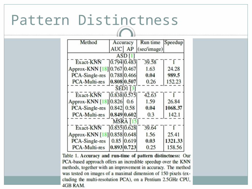
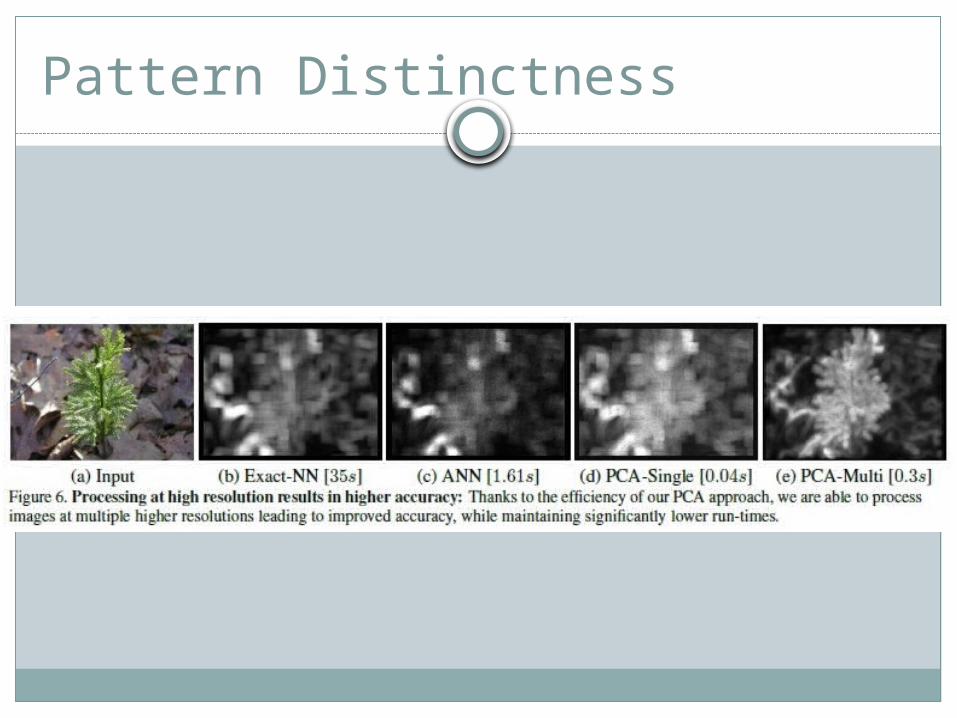
To measure accuracy, we report the Area-Under-the-Curve (AUC) and Average Precision (AP)(the higher the better).
Our approach is more accurate than both Exact-KNN and Approximate-KNN, while being significantly faster than both.
Pattern Distinctness
Pattern Distinctness
Pattern Distinctness
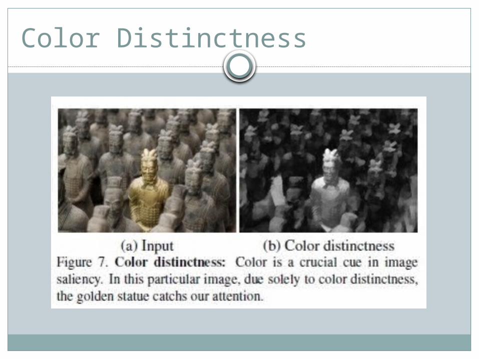
Color Distinctness
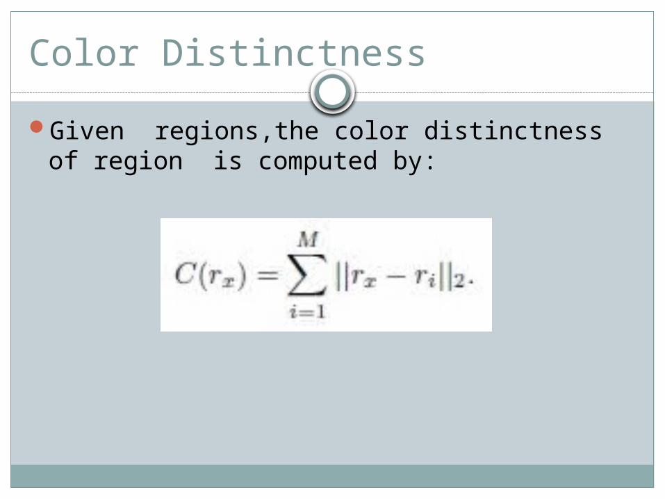
Given regions,the color distinctness of region is computed by:
Color Distinctness
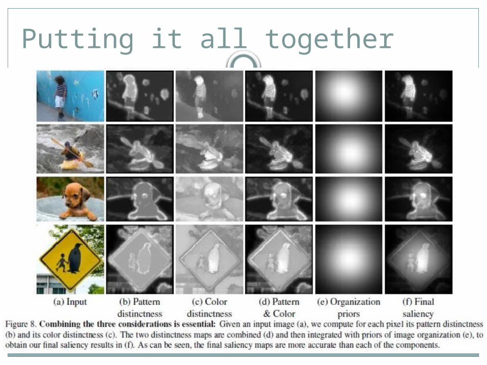
Putting it all together
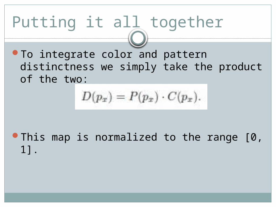
To integrate color and pattern distinctness we simply take the product of the two:
This map is normalized to the range [0, 1].
Putting it all together
We start by detecting the clusters of distinct pixels by iteratively thresholding the distinctness map using 10 regularly spaced thresholds between 0 and 1.
We compute the center-of-mass of each threshold result and place a Gaussian with = 10000 at its location.
We associate with each of these Gaussians an importance weight, corresponding to its threshold value.
In addition, to accommodate for the center prior, we further add a Gaussian at the center of the image with an associated weight of 5.
We then generate a weight map that is the weighted sum of all the Gaussians.
Putting it all together
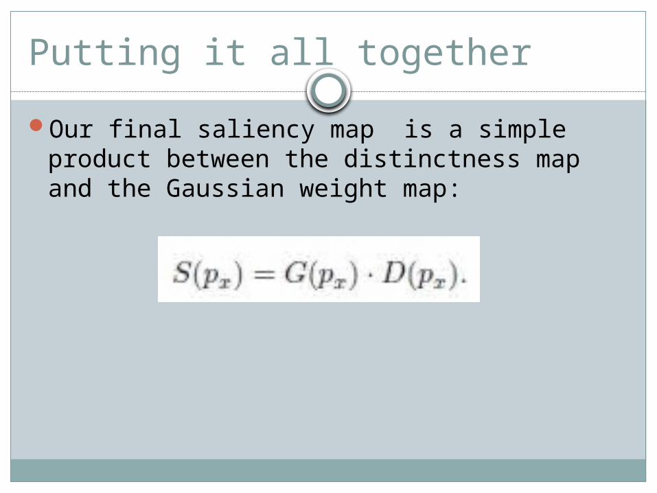
Our final saliency map is a simple product between the distinctness map and the Gaussian weight map:
Putting it all together
1. Accuracy2. Run-time3. Qualitative evaluation
Results
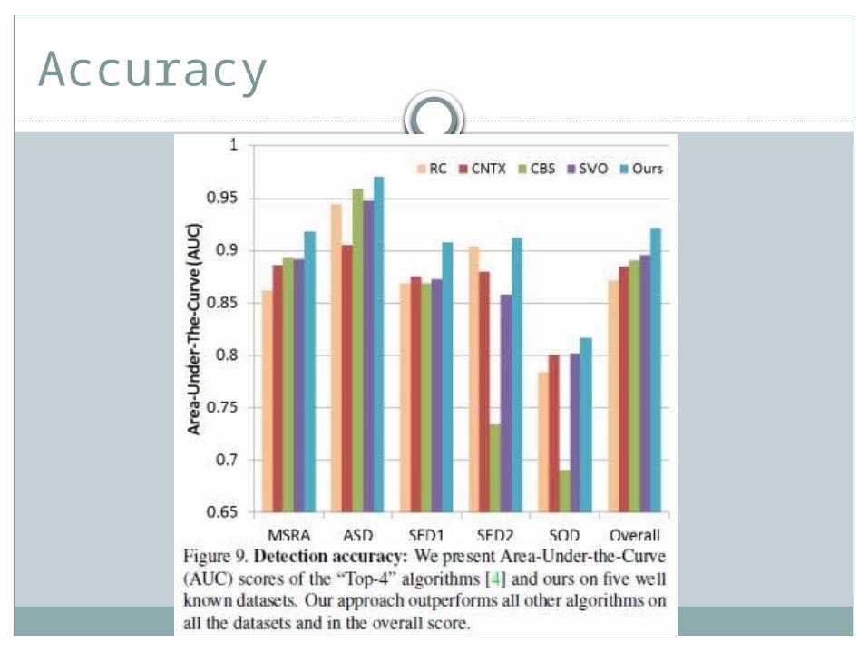
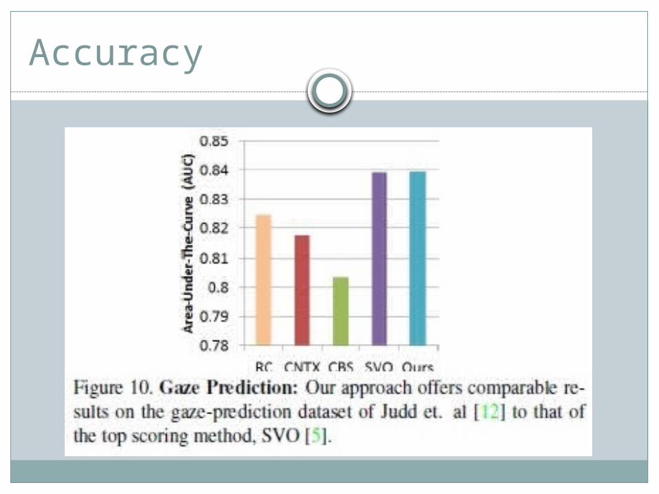
Accuracy
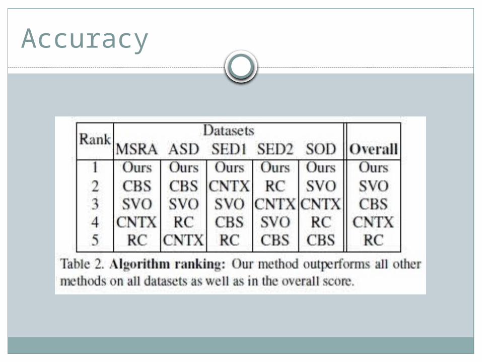
Accuracy
Accuracy
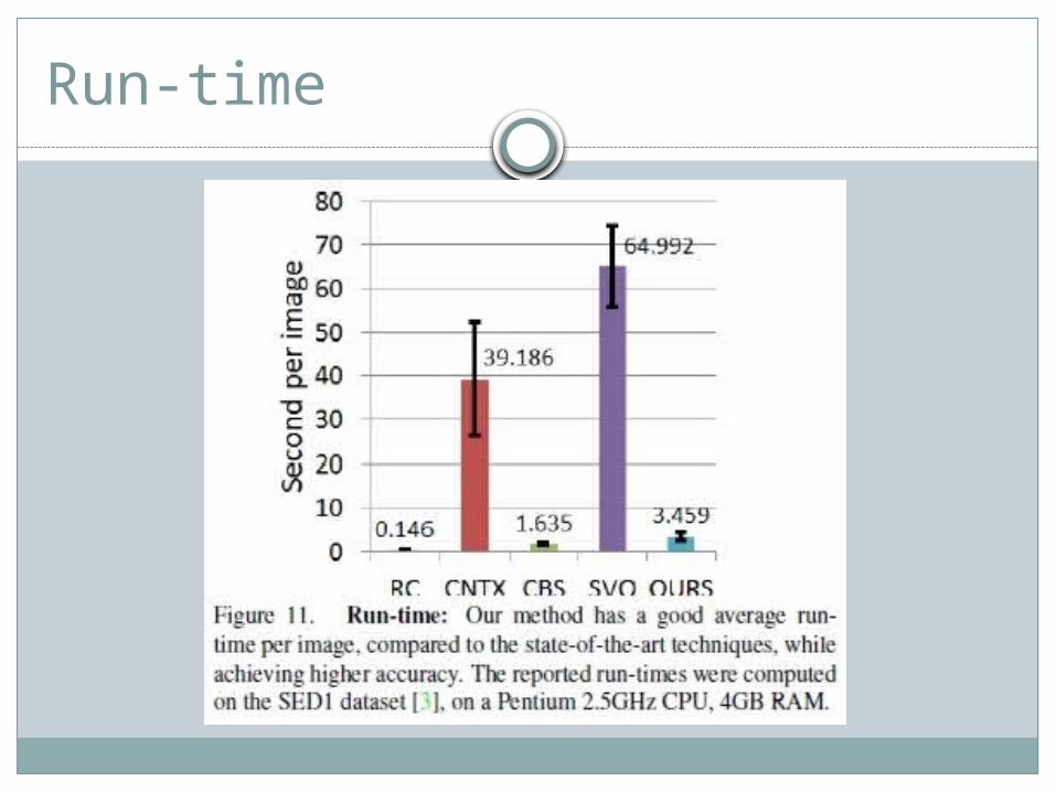
Run-time
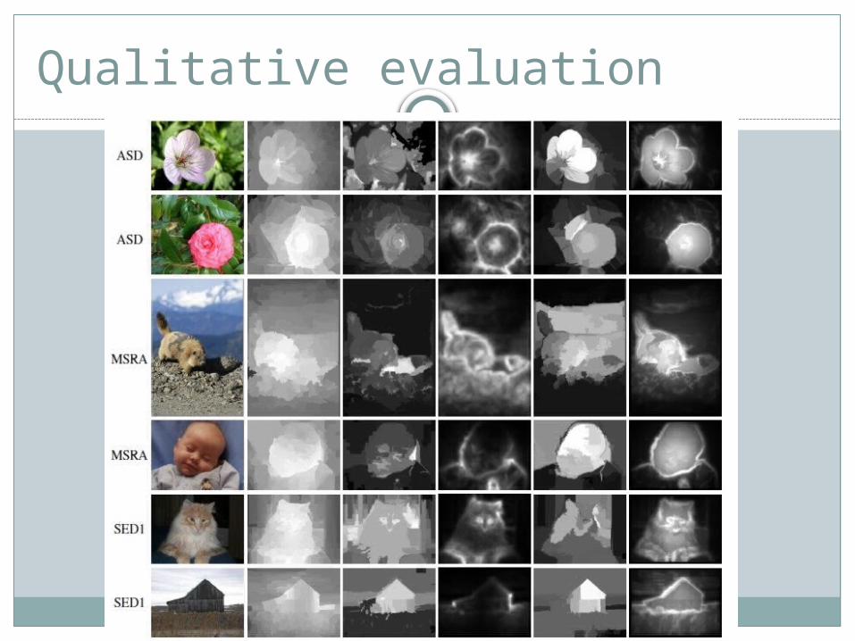
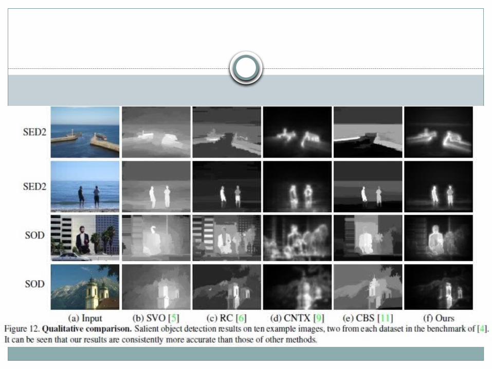
Qualitative evaluation
A drawback of our algorithm is not using hight-level cues, such as face detection or object recognition.
This can be easily addressed, by adding off-the-shelf recognition tools.
Discussion
Recommended