Wealth Effects on Consumption

in a Modified Life-Cycle Model'2 A. S. DEATON

Department of Applied Economics, Cambridge

I. INTRODUCTION In their original contributions [3] and [4], Modigliani and Brumberg showed that the maximization of an homogeneous inter-temporal utility function subject to a life-span budget constraint leads to a proportional relationship between consumption and permanent income. The exclusion of wealth from the utility function, justifiable in the absence of uncertainty, implies that the life time asset/liability plan is generated by divergences between the time profiles of human income and optimal consumption, the former being assumed outside the consumer's control. Given the standard " hill-shaped " time profile of human earnings, this will tend to lead to borrowing in the early years of productive activity, the repayment of these debts and further asset accumulation in middle age, succeeded by gradual dissaving through retirement until death. The close correspondence to reality of this aspect of the model is one of the grounds on which Modigliani and Brumberg justify their neglect of the problems associated with uncertainty.

It is the purpose of this paper to suggest that the role of wealth has been underestimated by ignoring uncertainty and to propose and test empirically a model which allows the wealth decision an independent part in the determination of consumption behaviour. In the next section, the model is presented as it concerns the individual; an analysis is made of wealth effects under perfect certainty and the considerable modifications needed in order to deal with uncertainty are discussed. In Section III, a macroeconomic version of the model is derived and tested against UK quarterly data. This section concludes with a discussion of the results and a numerical example designed to illustrate the magnitude of reactions to a change in stock market prices. Finally, in Section IV, the behaviour of the model in a steady growth environment is demonstrated and the steady growth savings ratio is tabu- lated as a function of the rate of growth of real income, the rate of inflation, and the rate of revaluation of wealth.

II. THE MICRO-MODEL

The instantaneous budget constraint facing the consumer may be written

wi(t) = rw(t)+yh(t)-c(t), ... (1) where w(t) is the market value of wealth at time t,

yh(t) is human earnings at time t, c(t) is consumption expenditure at time t.

A superimposed dot indicates the rate of change with respect to time t. r is the rate of reproduction of wealth and includes not only interest payments but also upward or down- ward revaluations in the market value of wealth. If we let t = 0 represent the present and

1 First version received September 1970; final version received October 1971 (Eds.). 2 The author is indebted to Professors J. R. N. Stone and D. G. Champernowne, Dr M. R. Fisher

and members of the Cambridge Growth Project for useful help and discussion. This paper has been improved greatly as a result of the comments of the anonymous referees of this journal.

443

444 REVIEW OF ECONOMIC STUDIES

t = L represent the time of death, we may multiply both sides of (1) by r exp (-rt) and integrate over the range t = 0 to t = L to derive a life time budget constraint. This yields,

L rL

r exp (-rt)c(t)dt = r exp (- rt)yh(t)dt + r{w(O) - exp (-rL)w(L)}. ...(2) o Jo

Taking the terms on the right hand side in order, the first is the return from human capital, or permanent human income; the second is the return from the difference between human capital owned in the present and discounted bequests, and can be called permanent non- human income. We shall call the sum of these terms permanent income, yP, and write

rL r { exp (-rt)c(t)dt = yP(O). ... (3)

0

Now in order to derive a consumption function from a budget constraint we need inform- ation on the consumer's preferences. We may proceed directly from (3), as do Modigliani and Brumberg, and assume that the time profile of consumption is independent of the level of permanent income (though not of the rate of reproduction of wealth). Thus, dropping the time suffix, which we may do as plans are being constantly remade, we have the propor- tional relationship

c = k(r)yP. _ *(4)

Unfortunately, under this formulation, it is not clear exactly how the constant of proportion- ality is determined and in order to analyse wealth effects, we need to know how it responds to changes in the rate of interest. In a regrettably unpublished article (but see [8, p. 79] for a brief exposition), Champernowne has shown that in a model where the consumer plans forward for all time, the assumption of a constant elasticity of marginal utility with respect to consumption leads to a precise algebraic formulation of the type we desire. We may relax the assumption of an infinite time horizon but preserve the main features of the model by assuming that the consumer maximizes

rL

u = { x exp (-6t)u{c(t)}dt ... (5)

subject to the constraint (1), where u is a time invariant utility function which is homo- geneous of degree j, where il is less than unity.' For maximization it is necessary that

au/ac = yo/'o exp {(3 - r)t}

where yo is an undetermined multiplier. Now au/ac is some function of c, say f(c), and we may suppose this function to have an inverse,

C = f - I[yo/do exp {(3-r)t}]

where f is homogeneous of degree (-0) with

0 = (I -1.

Applying Euler's theorem on homogeneous functions we reach

c(t) = 0(r - 6)c(t). ... (6)

Evidently, consumption grows steadily at a growth rate g which is positive or negative as r is greater than or less than 3. If we interpret 3 as the consumer's internal rate of discount, we have growth which is proportional to the difference between the internal and external rates of interest.

1 q, < 1 is necessary if a2U/ac2 is to be negative and au/sc positive. If 7 < 0, u is bounded above or in the terminology of Robertson and Champernowne, bliss is finite; this assumption can be used to rule out awkward cases if L is allowed to be infinite. It is not used here.

DEATON WEALTH EFFECTS 445

If we substitute (6) back into the budget constraint the proportionality relationship (4) follows immediately and we now have

with k = x{(exp x-1)rL}1 (7)

x = (g-r)L = (qr-3)OL. It is clear that we have sacrificed a considerable amount of the generality of the Modigliani/ Brumberg approach in order to get this far. However, one may perhaps hope that the dependence of k on r in this formulation is not untypical.

Since x is always at least as small as (exp x- 1), and since both are zero when x is zero, k is always positive for positive r and L. Furthermore, k is greater than or less than the reciprocal of rL as x is less than or greater than zero, i.e. as consumption grows slower or faster than the rate of interest. The meaning of this is clear; if g is equal to r, the con- sumer with L years to live will consume the Lth part of his total (discounted) resources in the current period. This may be thought of as the " neutral " situation; if g is less than r there is a bias towards greater present consumption, if g is greater than r, the opposite is true. But from (7), the inequality relationship between g and r is equivalent to that between ilr and 6. This is reasonable; the product of i and r is a measure, in terms of utility, of the benefits of postponing consumption whereas 3 is a measure of the cost.

The effects of changes in the rate of interest on consumption may now be studied directly, first via their effects on k and second via their effects on yP. Differentiating (7), with respect to r, we have

aklar = r-'[a/ax{x(exp x-1)- 11}0 - x{rL(exp x-1)}1]. Performing the internal differentiation and rearranging, we have'

ak/ar = O(r exp x-1)- 1 [bl/r-x{1-exp (-x)}], so if x iS positive,

exp(x)-1>0, x{1-exp(-x)}1>'1, ii>6/r,

and if x is negative the opposite inequalities hold. In either case the derivative is given by the product of a positive and a negative quantity and is thus negative for all x. This is the normal intertemporal substitution effect caused by shifts in the rate of interest changing the relative price of present vis-'a-vis future consumption. The analysis of the income effect is more complex and no definite result can be achieved without specifying the exact times at which the consumer expects his receipts and payments to occur. If we regard permanent income as the return on a capital sum formed by discounting income streams (i.e. non- human wealth is the title to specified future receipts and payments), then

L

yP = r exp (-rt)y(t)dt, 0

and rL

ayP/ar f (1- rt) exp (-rt)y(t)dt. ...(8)

This expression can clearly be either positive or negative depending on the size of r, L and the time profile of y(t). However, it can be seen that if r is less than the reciprocal of L and if y(t) is positive the integrand is always positive; given the normal range of values of r, the average remaining life span of the population and the considerable oversufficiency of this condition, it would be surprising if an increase in r did not have a positive income effect overall. Individuals for whom (8) is negative are almost certainly atypical; con- sumers who expect considerable receipts at a date far distant in the future or who inherit the commitment to pay off large debts are not the usual paradigms.

1 If x = 0, i.e. if 'qr = 8, neither this equation, nor equation (7) are defined. The corresponding formulae are k = (rL)-l and ck/9r = -r-2 [L-11+08]. Note that the latter is negative.

446 REVIEW OF ECONOMIC STUDIES

Thus, though in specific cases we may predict the net effects, in general, changes in the rate of reproduction of wealth (and hence in the value of wealth) give rise to two conflicting forces on current consumption, the relative size of which is not uniformly predictable.

It is possible to go on to discuss further the implications of this model but unless we admit uncertainty great demands will be made of the reader's credulity. But without the perfect certainty assumptions the model is not a viable framework for analysing wealth effects on consumption. Nevertheless, much of the model can be modified to meet our purpose.

While we admit that knowledge of income streams over the remainder of the life-span is normally unavailable, we accept that consumption plans are made some distance into the future. Permanent income is thus still an operative concept though it loses much of its exactness; this is no great disadvantage in empirical work as neither of the theoretical formulations above has a directly available equivalent. All we shall require below is that permanent income responds partially to current measured income and this is consistent with any length of planning horizon. We may further redefine the rate of reproduction of wealth as a long term expectational variable; we let it be that rate at which the consumer expects his assets to accumulate due to interest, dividends, and capital gains over his planning period. This rate will not now correspond to any observable rate, though once again we should expect it to be responsive to currently observed changes in events. Even so, if the planning period is long, it will probably vary little and then but slowly.

Having made these reservations, we might then be tempted to put the proportionality hypothesis to the test, either with k fixed or with k dependent on some interest rate variable. However, this would be to ignore one major modification yet needed; it is necessary to take account of the effects of uncertainty on the need to hold assets.

It is not at all obvious how this should be done. One possibility is to introduce a priori probability distributions of income and revaluations and allow the consumer to maximize the expected value of his utility function, now modified so as to include the consumer's attitude towards risk. This method, while of value in situations involving pure risk (i.e. portfolio selection), is of little use for dealing with the more general uncertainty which is involved here. This is too intangible to be characterized by a known set of probabilities attached to the various possible events; the probabilities themselves are subject to as much uncertainty as are the events.

A second possibility is to introduce the market value of wealth into the utility function and this has the advantage of making direct acknowledgement of the fact that consumers derive present utility from the possession of assets. Nevertheless, the difficulty of speci- fication remains extreme. The optimal level of wealth will depend not only upon consump- tion preferences and the degree of uncertainty, but also on age, marital status, number of children, and many other factors. Permanent income will also enter this formulation, as once again the budget constraint must be satisfied. We may thus write

w* = m(a, b)yP ...(9)

where an asterisk denotes a " desired " or optimal level and m is a function (with the dimension of time) of age a, and other relevant variables b.

We thus hypothesize that, under uncertainty, the consumer will attempt to reconcile the two possibly conflicting consumption plans

C* = k(a, r)yP ...(10.1)

W* = m(a, b)yP ... (10.2)

within his current budget constraint. Note first that this way of stating the problem is consistent with our second possibility, that of including wealth in the utility function. One can perhaps imagine a hierarchic system of utility maximization; the consumer derives his optimal consumption plan, ignoring wealth and uncertainty, and his optimal asset plan,

DEATON WEALTH EFFECTS 447

ignoring all but the most insistent needs of present consumption. He then uses some trade- off function to determine his actual behaviour. In this situation one would expect to find the value of k greater than the observed consumption/income ratio and the value of m greater than the observed wealth/income ratio.

Second, note that the formulation (10) includes the Modigliani-Brumberg perfect certainty model as a special case. This is when the consumer is either perfectly certain about the future or chooses to ignore uncertainty altogether. Here any wealth plan will be as good as any other wealth plan as far as (10.2) is concerned and (10.1), i.e. consumption plans alone, will determine his behaviour. In this case the value of m is derivable directly from k and the time profile of actual income receipts; this derivation is actually done by Modigliani and Brumberg. In the above formulation, however, the consumer is allowed more general behaviour and his need to optimize consumption over time can be modified by his need to protect himself by holding assets.

We cannot now develop the micro-model further without specifying the function m. It is neither practical nor useful to do this-any formulation general enough to be credible would almost certainly be unmanageable-and we shall instead continue by postulating a possible aggregation of equations (10) and from there developing a complete and empiric- ally testable model.

III. THE AGGREGATE MODEL AND EMPIRICAL RESULTS We postulate the aggregate relationships

C* =kyp ..(11

W* = mYP ... (11.2)

where capitals denote aggregates over all consumer units. In order to derive (11) from (10) we have assumed first, that all consumers face the same r and that for any given age group, the distributions of k and m about the group means are independent of the distribution of permanent income. The above equations then follow with,

k = E ki(ygp/Yp)

and m = Z

fi(yF/YP),

where the suffix refers to a particular age group and superimposed bars denote arithmetic means. Since we shall be estimating the model over quarterly data with a relatively short time span in all, it seems reasonable to assume that the age group shares in total permanent income are relatively constant. In any case, given the nature of the indices involved, this is unlikely to be a major source of error. Equally we should still expect the relationship between k and r to exist in a modified but similar form between E and r.

Permanent income is assumed to be generated in the usual way, i.e.

YP = AY+ (1 - A)E -1YP ...(12.1) where E` is the backward shift operator and A is the aggregate elasticity of income expectations. Note that no single consumer is assumed to conform to this relationship; no matter how each unit arrives at its estimate of permanent income, in aggregate (12.1) is assumed to hold. We are also here assuming constancy of r; more will be said of this below.

Furthermore, following Stone [9], we define permanent wealth, WP.

WP = yW+(1-1t)E-1WP ...(12.2) This variable will be used to replace wealth on the left hand side of (11.2). Because the micro-model specifies long term desired levels, the consumer will only be concerned with

448 REVIEW OF ECONOMIC STUDIES

wealth which is not regarded as transient. In other words, temporary revaluations are not regarded as contributing to the desired stock. Note that the original model is not excluded; u = 1 is a perfectly acceptable limiting case of (12.2).

It now only remains to specify how we expect the conflicting plans (11) to be reconciled within the budget constraint. We shall again do this at a global level and make no attempt to ascertain how each unit solves his problem as posed by (10). The economy is assumed to solve the problem as if its members acted in such a way as to minimize the global loss function,

F = a(C_kyp)2+P(EWP_myp)2 ...(13) subject to the budget constraint, thus reconciling as far as possible, discrepancies between the not necessarily consistent plans for consumption and wealth additions. We define the parameter oa as the ratio of ,B to a; it may be thought of as the relative marginal disutility of an extra unit of wealth relative to an extra unit of consumption when each is equally out of equilibrium. This parameter plays an important role in the subsequent analysis; if uncertainty is completely unimportant, we should expect oa to be zero; if, on the contrary, we can establish that oa is significantly positive then we have evidence that uncertainty has sufficient impact to allow wealth a modifying effect on consumption plans.

Since wealth is defined in constant price terms, the budget constraint may be written EW = (1 +r)-'(Y+ W+R-C) ...(14.1)

where t is rate of inflation from one period to the next and R are revaluations to wealth expected in the current period. In terms of the variables in the loss function, using (12.2) we have

(1 +2t)EWP+/tC = M(Y+R+ W)+(1 +2t)(1 - p)WP. ...(14.2)

We may now set up the Lagrangean in the usual way and after some manipulation the first order conditions give us a consumption function,

C = aC1YP+0C2WP+0C3(R + W+ Y), .. .(15) where

al= k-h)(1 + x)~

a'2 = Ci(l - ){(l + X)(1 + 7)}-

a'3 = X(1 +X)-1

x = o,I2(1 + )- 2.

Note that income is only an incidental determinant of consumption; the important deter- mining variables are permanent income, permanent wealth and total available resources. The relative importance of permanent income and permanent wealth is determined by the size of the parameter a, which, as we have seen, may be regarded as a measure of the importance of uncertainty. The function (15) is not dissimilar to that proposed by Stone [9] where consumption was postulated to be a function of the permanent and transient components of both wealth and income. This gave rise to six independent parameters as opposed to four in (15), i.e. (al, a2, a3 and A); this reduction is due to the " tighter " specification of our model and is of great value in avoiding problems of multicollinearity in estimation.

In order to fit equation (15) it was assumed that the parameters al, a2 and a3 remained constant throughout the data period. The level of 7, the rate of inflation, was held fixed at the average quarterly rate over the relevant period. The equation was estimated over a relatively short span of eleven years, 1955 to 1966, and over such a period we feel justified in ignoring changes in population, population structure, and tastes. Though rates of interest were not constant, when dividends and capital gains are taken into account along with the probability of long planning horizons and slowly changing expectations, the

DEATON WEALTH EFFECTS 449

effects on k are probably small enough to ignore. Similarly an ingrained expectation of price rises at just over 3 per cent. per year seems reasonable. One further assumption was made; since the model is being fitted quarterly, there is probably less error involved in letting actual revaluations stand proxy for the expected revaluations of (15) than in attempt- ing to estimate some much more complex (and largely arbitrary) expectational process.

Quarterly, seasonally adjusted, data on consumption, excluding purchases of consumer durables, on prices and on personal disposable income were taken from [2]; quarterly estimates of depreciation were made based on the annual data from [1], and these were deducted from the income series to give incomes net of depreciation. Allowance was also made for depreciation to consumer durables which themselves were included in the wealth stock. Data on quarterly personal wealth were taken from Roe [7], the series being based on the pioneering work of Revell [6], a work without which this sort of analysis would be impossible. Revaluations were calculated by deducting savings from the observed changes in the market value of wealth after allowing for depreciation. No attempt was made to seasonally adjust either this or the wealth series. Both sets of data are dominated by revaluations in stock and bond market assets and given the possibilities for arbitrage in both markets, it would be surprising were a true seasonal pattern allowed to persist. Any pattern detected by a mechanical adjustment mechanism would thus be almost certainly spurious.

To generate a fittable equation, (15) was multiplied by the double transform

{1 -(1 - A)E- '}{ -(1 -)E- 1} to remove the unobservable terms. This leaves us the equation

C = fl,E-'C+fl2E-2C+133Y+134E-lY+fl5E-2Y+16W

+fl7E'-W+fl8E-2W+flgR+l,OE-'R+fl,,E-2R ... (16) where the f, parameters are non-linear functions of the original variables. The regression was carried out by non-linear minimization of the residual sum of squares with respect to

2= k -- , -, i, and ,u. The method is a constrained version of the Gauss-Newton iterative procedure and is due to Marquardt [5]. Though we may seem to have lost much due to the complexity of such a fitting procedure and its attendant statistical uncertainties, we have gained a great deal in being able to test a complex hypothesis involving eleven 'independent' variables without the usual problems of collinearity.

In this case convergence was obtained after nine iterations and the parameter values with corresponding asymptotic standard errors were as follows

vk -i/= 0f91669 (0-03716) a = 0-00391 (0-00165) A = 0-07903 (0-03173)

,u = 1-16126 (0.14752)

R' = 0-99694 7t was fixed at 0 00766.

Several features of these results ought to be commented upon. First, note that the estimate of a is positive and is significantly greater than zero at the two per cent level of significance. We would thus seem justified in concluding that the evidence is consistent with there being a significant effect of uncertainty on aggregate consumption. This is perhaps the most important of the empirical conclusions.'

It is not possible to estimate k and mfi separately; however we can find pairs of values 1 A more powerful test of the model would clearly be an F or likelihood ratio test between the model as

estimated and the OLS free estimation of (16). Unfortunately the correlations between the variables in (16) are so strong that this cannot be done; some restrictions are necessary a priori in order to estimate the model at all. Experiments comparing the model to (16) estimated with various subgroups of the variables included failed to yield any F ratios significant at the 5 per cent level, to this extent the implied restrictions of the model would seem acceptable.

2F

450 REVIEW OF ECONOMIC STUDIES

consistent with the empirical estimates of il and a. One such pair is k = 1 and m = 21 quarters or five and a quarter years. Since the product of r and L is, on average, of the order of unity, this value of k would represent for an individual consumer, the " neutral " consumption case discussed above. This would be a very appealing simplification of the perfect certainty model. Furthermore, the observed ratio of wealth to income over the period was on average slightly less than four years; thus these two values satisfy exactly the theoretical properties required of them above.

The values of ) and ,u are perhaps less satisfactory. The very low estimate of ) implies a somewhat longer planning horizon than introspection would lead one to expect, and permanent income adjusts very slowly to measured income. On the other hand, the estimate of ,t is high; one is reluctant to believe that the destabilizing behaviour implied actually exists. More plausibly, either wealth has been incorrectly aggregated, or, since , is not significantly different from unity, permanent wealth is not distinguishable from actual wealth. This latter possibility was tested by re-estimating the model with ,I constrained to be unity. This gave new values of the other parameters as follows,

09 = 09O356 (0.03900) = 0 00503 (0-00195)

A = 0'08562 (0.03568) with R2 = 099685. The F-test associated with the imposition of the constraint takes the value 1-18 which is highly favourable for the constraint. We conclude then that the intro- duction of the concept of permanent wealth does not lead to any significant increase in our ability to explain aggregate consumption.

At this point it is necessary to insert a number of important statistical caveats. Even when ,u is constrained to take the value unity, the parameter estimate of ) is largely deter- mined by the relationship between the dependent variable and lagged values of itself. In the presence of serial correlation, the estimates (particularly that of A) could be subject to considerable bias even in OLS regression and though it is difficult to assess the properties of the estimates when non-linear techniques are used we are probably safe in assuming that matters are worse, not better. That autocorrelation exists is incontestable; the lag trans- forms used will generate a first or second order moving average error term, depending on whether or not it is constrained. But this assumes that the initial error is non-autocorrelated and in work on consumption functions this is unlikely to be so. This is not because of behavioural considerations but rather because of the possibility of consistent underestimation of personal income in the national income statistics. This would add a further dimension to the serial correlation problem. Finally, it is clear that the wealth series is probably subject to considerable errors of measurement which would not only cause trouble on their own account but would be echoed in the revaluation series.

The proper inclusion of all these possibilities into the structure of the model is clearly a major task, and its successful completion is beyond the scope of this paper. Equally it is not clear that minor corrections of the estimating equations or of the estimating procedure will substantially improve the parameter estimates. It would seem best therefore to accept the values tabulated as provisional and to accept modifications when more work has been done on the specific sources of error enumerated above.

We can use the estimates to derive the parameters of equations (16). This becomes, with ,u = 1,

C = 0 91438E -'C + 0-08191 Y - 0-00450E -'Y (0 03568) (0'03019) (9-00177)

+ 0 00493W - 000450E-'W + 0*00493R (0.00190) (0*00177) (0.00190)

- 0-00450E-'R. (0.00177)

DEATON WEALTH EFFECTS 451

(Standard errors are quoted for reference only; they are based on those of the structural coefficients and are not independent tests of the significance of the f coefficients.)

Orders of magnitude can be gauged from the following example. At the beginning of 1969 the Financial Times ordinary share index stood at over 500; over the next quarter there was a drop of approximately 6 per cent. followed by a further fall of 19 per cent. in the second quarter. At present, our quarterly data on wealth ceases at the end of 1966, and we can only estimate the impact of this on personal net worth. Likely figures are capital losses of ?115 billion and ?3043 billion in real terms in the two quarters. As a hypothetical example we shall compare the case of constant real wealth with the above depreciations, wealth being assumed to remain constant after the second fall. Income is the same in both cases. Substitution of these values in the above equation gives the follow- ing shortfalls in consumption (at 1958 prices) for the first four quarters; ?5-7 million, ?22-6 million, ?22-5 million and ?22-4 million. Thereafter the shortfall diminishes at 0*4 per cent. per quarter. Thus though the effect is small, it is long lasting, though in practice rapidly swamped by other factors. Perhaps we can conclude that in normal circumstances ignoring wealth effects causes little error; in times when stock market values change very rapidly, especially in financial crises, there is a significant impact. It is worth noting that wealth effects are certainly not large enough for any significant effect on employment via consumption due to a fall in the price of consumer goods; furthermore, periods of insuffi- cient effective demand are often characterized by low stock market prices and this would act in a manner to exacerbate rather than ameliorate the situation. This is not to say that a change in the long term expected rate of inflation could not have a more powerful impact, at least in the longer run, but this effect works not as a real balance effect, but through changing the parameters of the model. It is these long term considerations with which this paper concludes.

IV. STEADY GROWTH SOLUTIONS

We may rewrite (15) as an aggregate saving equation S = O-c1Yp- x3(R+ W)+(1-x3)Y-cc2Wp. ... (17)

We already have p = (1 + r)E-lp ... (18.1)

where p is the price level, to this we add Y= (1 +g)E-1Y ...(18.2)

R=pW ... (18.3)

i.e. income grows at a constant rate 9, and revaluations are a constant proportion of wealth. Note that p # r as the latter includes interest payments. From (12)

{1-(l-A)E-}YP AY= ... (19.1)

{1-(1-p)E-1}WP =PW ... (19.2) and the budget constraint can be written, substituting (18.3) in (14.1)

{(1l+n)-(1 +p)E-1}W = E-ls. ... (19.3)

Thus, substituting for R in (21) and multipjying both sides by the factor

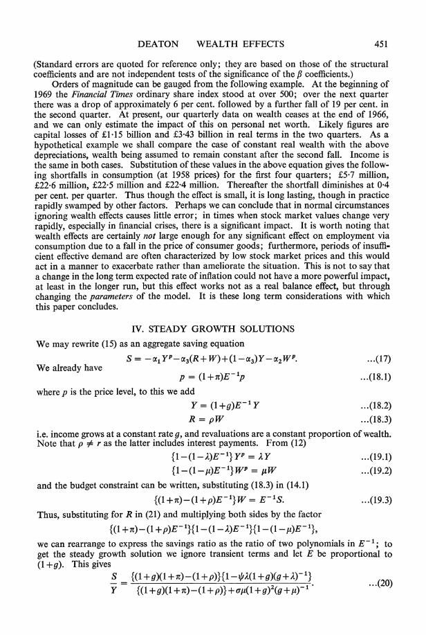
{(I +n)-(l +p)E- 1}{l -(I -A)E- 1}11-(I 1,t)E- 1b, we can rearrange to express the savings ratio as the ratio of two polynomials in E-1; to get the steady growth solution we ignore transient terms and let E be proportional to (1 +g). This gives

S ..{( +g)(l+r2)0(l+p)}{l 4 l+g)(g+i}(20)

Y {(l + g)(I + )-(1 + p)} + a(l + g)2(g + py 1**20)

452 REVIEW OF ECONOMIC STUDIES

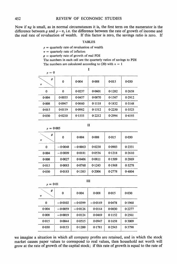
Now if rg is small, as in normal circumstances it is, the first term on the numerator is the difference between g and p - i, i.e. the difference between the rate of growth of income and the real rate of revaluation of wealth. If this factor is zero, the savings ratio is zero. If

TABLES

p = quarterly rate of revaluation of wealth r = quarterly rate of inflation

g = quarterly rate of growth of real PDI The numbers in each cell are the quarterly ratios of savings to PDI The numbers are calculated according to (20) with a = 1

I p = 0

X \ 0 0004 0008 0-015 0030

0 0 0-0237 0-0601 0-1282 0-2658

0 004 0 0035 0 0457 0-0870 0-1567 0*2912

0-008 0 0967 0-0660 0-1118 0-1832 0-3148

0.015 0 0119 0-0982 0-1512 0-2250 0*3523

0 030 0 0210 0-1555 0 2212 0 2994 0-4193

II p = 0 005

0 0 004 0-008 0 015 0 030

0 - 0-0048 -0-0063 0-0238 0 0903 0-2331

0 004 -0 0009 0-0181 0-0536 0-1218 0'2610

0-008 0-0027 0-0406 0-0811 0 1509 0 2869

0 015 0 0083 0-0760 0-1243 0-1968 0-3278

0 030 0-0183 0-1385 0-2006 0-2778 0 4004

III p = 0-01

g 0 0004 0008 0 015 0030

0 -0-0102 -0-0399 -0-0169 0-0478 0 1968

0 004 -0 0059 -0-0126 0 0164 0-0830 0-2277

0 008 -0 0019 0-0124 0-0469 0 1152 0-2561

0015 0*0044 00515 00947 01658 03009

0 030 0 0153 0 1200 0-1781 0 2543 0 3798

we imagine a situation in which all company profits are retained, and in which the stock market causes paper values to correspond to real values, then household net worth will grow at the rate of growth of the capital stock; if this rate of growth is equal to the rate of

DEATON WEALTH EFFECTS 453

growth of real disposable income households will not save. In this case saving and invest- ment are equilibriated within the company sector.

Even when this is not so, (20) leaves plenty of scope for the savings ratio to adapt to whatever ratio of growth is taking place. It is clear that there is a role for both the rate of interest and the rate of inflation in this mechanism and the equation highlights part of the contribution of these variables towards the growth process. A full analysis would require specification of corporate saving and investment functions and there is no wish to trespass so far afield in this paper.

In the tables which follow some values calculated from (20) are presented. The function seems well behaved and note that values within the normal range of experience are very close to those actually observed. It is important to note how very responsive the savings ratio is to the growth rate; for example, with p = 0 005 and 7t = 0-008, a 12-6 per cent. annum growth rate in real personal disposable income will induce a savings ratio of over 28 per cent. compared with just over 8 per cent. at a growth rate of 3 2 per cent. The higher figures, though calculated on UK data, show a remarkable resemblance to recent Japanese experience. In the light of these results it would seem very unlikely that growth, in this or any other similar country is being or has been retarded by an inadequate household savings ratio.

REFERENCES

[1] Central Statistical Office. National lncome and Expenditure (1968).

[2] Central Statistical Office. Economic Trends (October 1968).

[3] Modigliani, F. and Brumberg, R. " Utility Analysis and the Consumption Function: An Interpretation of Cross Section Data ", in K. K. Kurihara (ed.) Post Keynesian Economics (Allen and Unwin, 1955).

[4] Modigliani, F. and Brumberg, R. "Utility Analysis and Aggregate Consumption Functions: An Attempt at Integration" (unpublished).

[5] Marquardt, D. W. " An Algorithm for Least-Squares Estimation of Non-Linear Parameters ", Journal of the Society of Industrial and Applied Mathematics, 2, No. 2 (1963).

[6] Revell, J. R. S. The Wealth of the Nation (Cambridge University Press, 1967).

[7] Roe, A. R. " A Quarterly Series of Personal Sector Assets and Liabilities ", Depart- ment of Applied Economics, Cambridge, internal paper.

[8] Robertson, Sir D. H. Lectures on Economic Principles Vol. II (Staples Press, London, 1958).

[9] Stone, J. R. N. " Spending and Saving in Relation to Income and Wealth ", L'industria No. 4 (1966).