CWP-784October 2013
Wavefield tomography using image-warping
Advisor: Prof. Paul Sava Committee Members: Prof. Dave Hale Prof. André Revil Prof. John Scales Prof. Luis Tenorio
- Doctoral Thesis - Geophysics
Center for Wave PhenomenaColorado School of MinesGolden, Colorado 80401
303.384.2178 http://cwp.mines.edu
Francesco Perrone
Defended on October 16, 2013


WAVEFIELD TOMOGRAPHY USING
IMAGE-WARPING
by
Francesco Perrone


ABSTRACT
The main objective of this thesis is to study new methods for estimating the macro
velocity model, which controls the wave kinematics, in the context of reflection seismology.
Migration velocity analysis evaluates the quality of the velocity model used for imaging
seismic data by comparing images of the subsurface structures as a function of extension
parameters, such as offset, reflection angle, or shot-index. The angle domain has proved to be
a suitable domain for velocity analysis because of its robustness against the noise introduced
by the migration operator and against the ambiguities due to complex wave propagation in
the subsurface. Nonetheless, angle gathers require an extra computational effort especially in
full azimuth 3D scenarios. On the other hand, most migration algorithms naturally process
the reflection data and output images in the shot-domain, which is usually regarded as a poor
option for velocity analysis. The ability to extract reliable information about the velocity
model from single-experiment images has value not only for the construction of macro velocity
models for imaging but also for the regularization of high-resolution data-fitting techniques
in a way that is compliant with the physics of wave propagation.
In this thesis, I investigate how to make shot-domain velocity analysis algorithms more
robust by exploiting the coherency of the structural features in the migrated domain and
using the concept of image-warping. I link the difference between two migrated images
with the concept of image-warping and show that with image-warping, one can obtain an
approximation of the image difference that is less sensitive to the distance between the shot
points. I use the image-warping approximation of the standard image difference as the input
of a linearized inversion scheme to reconstruct the velocity anomaly in the migration model.
The linearized inversion is based on one-way migration algorithms and relies on a series of
assumptions about the strength of the perturbation in the wavefields and in the model. In
order to remove these assumptions, I use the insight gained about the relationship between
iii
the orientation of the structural features in the image and the warping vector field to design
an optimization problem that does not involve any up-front linearization of the propagation
operator. Using adjoint-state techniques, I was able to compute the gradient of the objective
function and thus implement a two-way wavefield tomography scheme. The basic building
block of my tomography algorithm is the measure of the apparent displacement between
two nearby shot gathers along the normal direction to the imaged reflector. Because no
stacking of partial images is needed to obtain the measure of velocity error, my approach
is intrinsically shot-based. This feature of the error measure and inversion scheme allows
one to reconstruct errors in the migration velocity from a minimum number of experiments.
I show how this approach can reconstruct, using a single experiment, the anomaly in a
hydrocarbon reservoir that undergoes depletion because of production. The measure of local
apparent displacements with penalized local correlations proves to be effective in scenarios
where the geometry of the reflectors is simple and the orientation of the structural features
can be unambiguously computed. Moreover, penalized local correlations are particularly
sensitive to the shot distance for shallow interfaces and may suffer from crosstalk due to other
reflectors falling in the same correlation window. Following these considerations and using
the relationship between image difference and image-warping, I show that image-warping can
be used to modify the expression of the adjoint sources for standard differential semblance
optimization to make the method robust against cycle skipping in the image domain even
with strong errors in the velocity model.
iv

TABLE OF CONTENTS
ABSTRACT . . . . . . . . . . . . . . . . . . . . . . . . . . . . . . . . . . . . . . . . . iii
LIST OF FIGURES . . . . . . . . . . . . . . . . . . . . . . . . . . . . . . . . . . . . . ix
ACKNOWLEDGMENTS . . . . . . . . . . . . . . . . . . . . . . . . . . . . . . . . . xvii
DEDICATION . . . . . . . . . . . . . . . . . . . . . . . . . . . . . . . . . . . . . . . . xx
CHAPTER 1 INTRODUCTION . . . . . . . . . . . . . . . . . . . . . . . . . . . . . . . 1
1.1 Velocity Model Building Techniques . . . . . . . . . . . . . . . . . . . . . . . . . 2
1.2 Thesis Organization . . . . . . . . . . . . . . . . . . . . . . . . . . . . . . . . . . 8
CHAPTER 2 LINEARIZED WAVE-EQUATION MIGRATION VELOCITYANALYSIS BY IMAGE-WARPING . . . . . . . . . . . . . . . . . . . . 12
2.1 Summary . . . . . . . . . . . . . . . . . . . . . . . . . . . . . . . . . . . . . . 12
2.2 Introduction . . . . . . . . . . . . . . . . . . . . . . . . . . . . . . . . . . . . . 13
2.3 Image Similarity, Warping, and Velocity Errors . . . . . . . . . . . . . . . . . 14
2.3.1 The Semblance Principle . . . . . . . . . . . . . . . . . . . . . . . . . . 15
2.3.2 Image Difference, Image Warping, and Image Perturbation . . . . . . . 17
2.3.3 Wave-Equation Migration Velocity Analysis . . . . . . . . . . . . . . . 20
2.3.4 Workflow . . . . . . . . . . . . . . . . . . . . . . . . . . . . . . . . . . 23
2.4 Numerical Examples . . . . . . . . . . . . . . . . . . . . . . . . . . . . . . . . 24
2.4.1 Sensitivity to Cycle-Skipping and Backprojections . . . . . . . . . . . . 27
2.4.2 Inversion Test . . . . . . . . . . . . . . . . . . . . . . . . . . . . . . . . 29
2.4.3 Local Marmousi Inversion . . . . . . . . . . . . . . . . . . . . . . . . . 32
v

2.5 Discussion . . . . . . . . . . . . . . . . . . . . . . . . . . . . . . . . . . . . . . 36
2.6 Conclusions . . . . . . . . . . . . . . . . . . . . . . . . . . . . . . . . . . . . . 39
2.7 Acknowledgments . . . . . . . . . . . . . . . . . . . . . . . . . . . . . . . . . . 40
CHAPTER 3 WAVEFIELD TOMOGRAPHY BASED ON LOCAL IMAGECORRELATIONS . . . . . . . . . . . . . . . . . . . . . . . . . . . . . . 41
3.1 Summary . . . . . . . . . . . . . . . . . . . . . . . . . . . . . . . . . . . . . . 41
3.2 Introduction . . . . . . . . . . . . . . . . . . . . . . . . . . . . . . . . . . . . . 42
3.3 Theory . . . . . . . . . . . . . . . . . . . . . . . . . . . . . . . . . . . . . . . . 45
3.3.1 Image Correlation Objective Function . . . . . . . . . . . . . . . . . . . 45
3.3.2 Computation of the Gradient with the Adjoint-State Method . . . . . . 51
3.3.3 Adjoint Sources . . . . . . . . . . . . . . . . . . . . . . . . . . . . . . . 53
3.3.4 Flat Reflector in a Constant Velocity Medium . . . . . . . . . . . . . . 55
3.4 Examples . . . . . . . . . . . . . . . . . . . . . . . . . . . . . . . . . . . . . . 58
3.4.1 Synthetic Laterally Heterogeneous Model . . . . . . . . . . . . . . . . . 58
3.4.2 Real Data . . . . . . . . . . . . . . . . . . . . . . . . . . . . . . . . . . 61
3.5 Discussion . . . . . . . . . . . . . . . . . . . . . . . . . . . . . . . . . . . . . . 63
3.6 Conclusions . . . . . . . . . . . . . . . . . . . . . . . . . . . . . . . . . . . . . 71
3.7 Acknowledgments . . . . . . . . . . . . . . . . . . . . . . . . . . . . . . . . . . 72
CHAPTER 4 SHOT-DOMAIN 4D TIME-LAPSE SEISMIC VELOCITYANALYSIS USING APPARENT IMAGE DISPLACEMENTS . . . . . 73
4.1 Summary . . . . . . . . . . . . . . . . . . . . . . . . . . . . . . . . . . . . . . 73
4.2 Introduction . . . . . . . . . . . . . . . . . . . . . . . . . . . . . . . . . . . . . 74
4.3 Theory . . . . . . . . . . . . . . . . . . . . . . . . . . . . . . . . . . . . . . . . 75
4.4 Synthetic Depletion Model . . . . . . . . . . . . . . . . . . . . . . . . . . . . . 77
vi

4.4.1 Full-Aperture, Repeatable Survey . . . . . . . . . . . . . . . . . . . . . 82
4.4.2 Limited-Aperture, Repeatable Survey . . . . . . . . . . . . . . . . . . . 86
4.4.3 Limited-Aperture, Non-repeatable Survey . . . . . . . . . . . . . . . . 90
4.5 Discussion . . . . . . . . . . . . . . . . . . . . . . . . . . . . . . . . . . . . . . 90
4.6 Conclusions . . . . . . . . . . . . . . . . . . . . . . . . . . . . . . . . . . . . . 95
4.7 Acknowledgment . . . . . . . . . . . . . . . . . . . . . . . . . . . . . . . . . . 96
CHAPTER 5 IMAGE-WARPING WAVEFORM TOMOGRAPHY . . . . . . . . . . . 97
5.1 Summary . . . . . . . . . . . . . . . . . . . . . . . . . . . . . . . . . . . . . . 97
5.2 Introduction . . . . . . . . . . . . . . . . . . . . . . . . . . . . . . . . . . . . . 98
5.3 Theory . . . . . . . . . . . . . . . . . . . . . . . . . . . . . . . . . . . . . . . 102
5.3.1 Adjoint-State Method, Demigration, and Iterative NonlinearInversion . . . . . . . . . . . . . . . . . . . . . . . . . . . . . . . . . . 104
5.4 Numerical Examples . . . . . . . . . . . . . . . . . . . . . . . . . . . . . . . 106
5.4.1 Horizontal Reflector . . . . . . . . . . . . . . . . . . . . . . . . . . . 106
5.4.2 Highly Refractive Model and Migration Failure . . . . . . . . . . . . 111
5.4.3 Marmousi Model . . . . . . . . . . . . . . . . . . . . . . . . . . . . . 113
5.5 Discussion . . . . . . . . . . . . . . . . . . . . . . . . . . . . . . . . . . . . . 125
5.6 Conclusions . . . . . . . . . . . . . . . . . . . . . . . . . . . . . . . . . . . . 128
5.7 Acknowledgments . . . . . . . . . . . . . . . . . . . . . . . . . . . . . . . . . 129
CHAPTER 6 CONCLUSIONS AND SUGGESTIONS . . . . . . . . . . . . . . . . . 130
6.1 Main Conclusions . . . . . . . . . . . . . . . . . . . . . . . . . . . . . . . . . 130
6.1.1 Image-Warping and Differential Semblance . . . . . . . . . . . . . . . 130
6.1.2 Geometrical Relationship between Structural Information andWarping . . . . . . . . . . . . . . . . . . . . . . . . . . . . . . . . . . 130
vii
6.1.3 Inversion of Apparent Displacements in the Image Domain . . . . . . 131
6.1.4 Superiority of Warping Vectors over Penalized Correlations . . . . . . 131
6.2 Future Research and Suggestions . . . . . . . . . . . . . . . . . . . . . . . . 132
6.2.1 Artifact-free Migration Algorithm . . . . . . . . . . . . . . . . . . . . 132
6.2.2 Warping Vector Field Calculation . . . . . . . . . . . . . . . . . . . . 132
6.2.3 Bi-objective FWI/MVA Optimization . . . . . . . . . . . . . . . . . . 133
REFERENCES CITED . . . . . . . . . . . . . . . . . . . . . . . . . . . . . . . . . . 134
APPENDIX A - COMPUTATION OF THE SOURCE AND RECEIVER ADJOINTSOURCE . . . . . . . . . . . . . . . . . . . . . . . . . . . . . . . . . 142
APPENDIX B - DIRECT ADJOINT-STATE CALCULATIONS FOR VECTORDISPLACEMENTS . . . . . . . . . . . . . . . . . . . . . . . . . . . 146
APPENDIX C - PERMISSION TO INCLUDE CO-AUTHORED MATERIAL . . . . 150
C.1 Request of Permission . . . . . . . . . . . . . . . . . . . . . . . . . . . . . . 150
C.2 Permission by Nicola Bienati, Eni E&P . . . . . . . . . . . . . . . . . . . . . 151
C.3 Permission by Clara Andreoletti, Eni E&P . . . . . . . . . . . . . . . . . . . 151
C.4 Permission by Jacopo Panizzardi, Eni E&P . . . . . . . . . . . . . . . . . . . 152
viii

LIST OF FIGURES
Figure 2.1 Migrated images can in principle be ordered in a hypercube andindexed by spatial location x, experiment number e, and extensionparameter α. By staking along one of the axes we reduce thedimensionality of the data and are able to analyze them. For example,we can stack along the extension parameter axis (e.g., reflection angle)and evaluate model accuracy by measuring the semblance at discretepositions in space between images corresponding to all experimentindices (a). Alternatively, by slicing together images from allexperiments, we obtain common-image gathers (e.g., angle-domaincommon-image gathers), which we usually analyze at fixed spatiallocations (b). A third option is to stack over the extension parameterand to analyze all points in the image for two (or a small number of)images obtained from nearby experiments (c). This last solution iswhat we propose in this paper. . . . . . . . . . . . . . . . . . . . . . . . . 15
Figure 2.2 Horizontal density interface imaged using a single shot at x = 2 km and800 receivers spaced 10 m at every grid point at the surface. The anglebetween the dip (solid arrows) and displacement vector field (dashedarrow) indicates a velocity error: (a) velocity too low, (b) correctvelocity, and (c) velocity too high. The displacement vector field iscomputed using a second image obtained from a shot located atx = 2.05 km. . . . . . . . . . . . . . . . . . . . . . . . . . . . . . . . . . . 19
Figure 2.3 Vertical section of a 3D model with azimuthal symmetry. (a) Densitymodel, (b) background slowness model, and (c) slowness anomaly. . . . . 25
Figure 2.4 (a), (c), and (e) show the backprojection of image perturbations for apositive value of the anomaly in Figure 2.3(c). The image perturbationsare obtained by forward WEMVA operator, image-warping, and imagedifference respectively. (b), (d), and (f) show the backprojectionsobtained for a negative anomaly. Image-warping consistently producessmoother backprojections that better approximate the ideal cases in (a)and (b). The oscillations in the backprojections of image differences areconnected with cycle-skipping problems. . . . . . . . . . . . . . . . . . . . 26
Figure 2.5 Model for the inversion test: (a) stack of layers with alternating valuesof density (b) correct slowness model. . . . . . . . . . . . . . . . . . . . . 28
Figure 2.6 Slowness model: (a) initial and (b) inverted after 13 nonlinear iterations. . 28
ix
Figure 2.7 Migrated images: (a) image obtained with the initial velocity modeland (b) after 13 velocity updates. The image in (b) is obtained after 13nonlinear iterations; every linearized problem involves five iterations ofconjugate gradient. Note the better focusing of the image. . . . . . . . . . 30
Figure 2.8 Comparison of the initial (dotted line), inverted (dashed line), andexact (solid line) slowness model at (a) x = 2.5 km and (b) x = 5.5 km.The inversion reduces the anomaly but does not eliminate it.Nonetheless, the reflectors in Figure 2.7(b) are flattened. . . . . . . . . . 31
Figure 2.9 The decrease of the energy of the image perturbation indicates that weare approaching the correct model. We stopped the inversion after 13iterations because the objective function starts oscillating, whichindicates that we reached a minimum of the objective function. . . . . . . 31
Figure 2.10 Macro slowness model (a) for the Marmousi dataset and (b) slownessperturbation for the model in (a). . . . . . . . . . . . . . . . . . . . . . . 32
Figure 2.11 Image obtained using the correct slowness model (a), initial migratedimage (b), migrated image after 20 nonlinear iterations (c). Weconsider 12 shots, evenly spaced by 0.04 km at the surface; the firstshot is positioned at x = 0.96 km. The receivers are are spaced 0.008km on the surface and they are located at every grid point. Observe theimproved continuity of the bottom reflector and the correction of thedistortion of the middle dipping interfaces at a lateral position aboutx = 2 km. . . . . . . . . . . . . . . . . . . . . . . . . . . . . . . . . . . . 33
Figure 2.12 (a) Exact slowness perturbation and (b) inverted anomaly after 20iterations of linearized migration velocity analysis. We correctly recoverthe location and magnitude of the perturbation. . . . . . . . . . . . . . . 34
Figure 2.13 Comparison of the initial (dotted line), inverted (dashed line), andexact (solid line) slowness model at x = 2.5 km. Observe that inversioncorrects the large discrepancy between the initial and correct model. . . . 35
Figure 2.14 The energy of the image perturbation decreases rapidly and reachesconvergence. . . . . . . . . . . . . . . . . . . . . . . . . . . . . . . . . . . 36
Figure 3.1 Relationship between the dip field and the apparent displacement: dip(solid) and displacement (dashed) vector fields for different values ofslowness error for a single horizontal reflectors: (a) ∆m
m= 10%, ∆m
m= 0,
and (c) ∆mm
= 10%. The correct slowness value is 0.5 s/km. . . . . . . . . 47
x

Figure 3.2 Measure of the relative displacement between two images usingpenalized local correlations. We consider 2 images from nearbyexperiments of the reflector in Figure 3.1; each row (from top tobottom) represents a different model: too high, correct, and too low;the columns show (from left to right) the local correlation panel, thepenalty operator used, and the penalized local correlation. For eachmodel, we pick a point on the reflector with lateral coordinatex = 3.5 km. The vertical coordinate changes as a function of modelparameters because the depth of the reflector changes. Observe theasymmetry of the penalized local correlations for the wrong models: themean value (i.e., the stack over the correlation lags) of the penalizedcorrelations gives us a measure of the relative shift between two images. . 49
Figure 3.3 Values of the objective function for different errors in the slownessmodel. We consider constant perturbations ranging from −10% to 10%of the exact value (0.5 s/km). . . . . . . . . . . . . . . . . . . . . . . . . 51
Figure 3.4 For the three cases in Figure 3.1, we compute the shifts r (x) accordingto equation 3.4. The sign of the shifts indicates the relativedisplacement of one image with respect to the other. . . . . . . . . . . . . 56
Figure 3.5 Gradient of the correlation objective function for a slowness model thatis too low (a), correct (b), and too high (c). The slowness squared erroris constant everywhere and equal to 10% of the background. Thedistance between the two shots is 60 m. We consider three shots andcomputed the gradient using the wavefields of the central experiment. . . 57
Figure 3.6 Velocity model used to generate the full-acoustic data. Absorbingboundary conditions have been applied at all sides of the model. Thelighter shades of grey indicate faster layers. The top layer has velocityof water (1.5 km/s). . . . . . . . . . . . . . . . . . . . . . . . . . . . . . . 58
Figure 3.7 Initial velocity model (a), associated migrated image (b), andshot-domain common-image gathers. The reflectors are severelydefocused and mispositioned. Observe the curvature of thecommon-image gathers that shows how different experiments image thereflectors at different depths. . . . . . . . . . . . . . . . . . . . . . . . . . 59
Figure 3.8 Velocity model after 15 iterations of waveform inversion (a), migratedimage (b), and shot-domain common-image gathers (c). Observe theimproved focusing and positioning of the reflectors. The common-imagegathers show that the images are invariant in the shot direction and themodel is thus kinematically correct. Observe the profile of the variouslayers in the reconstructed model. . . . . . . . . . . . . . . . . . . . . . . 62
xi

Figure 3.9 Evolution of the objective function with iterations. Observe the sharpdecrease of the objective function and the rapid convergence to akinematically accurate model. . . . . . . . . . . . . . . . . . . . . . . . . 63
Figure 3.10 Initial migration model and migrated image. . . . . . . . . . . . . . . . . 64
Figure 3.11 Final migration model and migrated image. The sections inFigure 3.10(b) and Figure 3.11(b) are displayed on the same color scale.Observe the increased amplitude of the reflectors due to better focusing. . 65
Figure 3.12 Shot-domain CIGs computed for the incorrect model at (a) x = 12 km,(b) x = 13 km, (c) x = 14 km, and (d) x = 15 km, and gatherscomputed after inversion at the same locations ((e), (f), (g), and (h)).The gathers are flattened by the inversion procedure, i.e. the reflectorsare invariant with respect to shot index. . . . . . . . . . . . . . . . . . . . 66
Figure 3.13 Angle-domain common-image gathers (ADCIGs) computed at severallateral positions (a) before, and (b) after inversion. After inversion thegathers are flatter, which indicates a more kinematically accuratemigration model. . . . . . . . . . . . . . . . . . . . . . . . . . . . . . . . 67
Figure 3.14 The evolution of the objective function shows that the algorithmconverges after about 80 iterations. . . . . . . . . . . . . . . . . . . . . . 68
Figure 4.1 Reservoir geometry after . Pore-pressure (PP = Pfluid) reduction occursonly within the reservoir, resulting in an anisotropic velocity field dueto the excess stress and strain. The reservoir is comprised of andembedded in homogeneous Berea sandstone (VP = 2300 ms−1,VS = 1456 ms−1, ρ = 2140 kgm−3). The Biot coefficient (α) for thereservoir is 0.85. Velocities in the model are reduced by 10% from thelaboratory values to account for the difference between static anddynamic stiffnesses in low-porosity rocks. The change in pore pressure∆Pfluid is expressed as a percentage ξ of the confining pressure Pcon. . . . 79
Figure 4.2 (a) Density model used to simulate the reflecting interfaces. (b) Velocitymodel of the depleted reservoir. The original model is homogenous with2.07 km/s velocity. Observe the characteristic shape of the anomalywith increasing velocity inside the reservoir (because of compaction)and decreasing velocity outside the reservoir (because of tensile strain). . 80
Figure 4.3 Sensitivity of the penalized local correlation objective function todifferent depletions of the reservoir. Observe the lost of sensitivity whenthe reservoir is strongly depleted. For this sensitivity study, we use afull and perfectly repeatable acquisition. . . . . . . . . . . . . . . . . . . . 81
xii

Figure 4.4 (a) Baseline data and (b) difference between monitor data simulated inthe depleted reservoir and baseline. The acquisition is perfectlyrepeatable, the source location is x = 1.5 km at the surface, andreceivers are at every grid point at z = 0 km. The change in polarityfor the shallowest events is due to the different sign of the velocityperturbation. . . . . . . . . . . . . . . . . . . . . . . . . . . . . . . . . . . 83
Figure 4.5 (a) Migrated monitor image obtained using the baseline model and (b)migrated monitor image after inversion with full receiver coverage atthe surface. The central and deeper reflectors are moved downward,which the shallowest interface is pulled up. The migration artifacts aredue to truncation of the acquisition and critical reflections (headwaves)from the anomaly in the depleted reservoir. . . . . . . . . . . . . . . . . 84
Figure 4.6 (a) Actual time-lapse model perturbation and (b) inverted perturbationafter 60 iterations of wavefield tomography with full receiver coverageat the surface. Notice that we are able to correctly image the anomalyand also constrain its lateral extent at about x = 2 km. . . . . . . . . . . 85
Figure 4.7 (a) Initial estimated shifts and (b) estimated shifts after 60 iterations ofwavefield tomography. Black indicates positive (downward) shifts andwhite represents negative (upward) shifts. Inversion matches thebaseline and monitor images and reduces the shifts between them. Thestrong residual after inversion at about x = 2.7 km for the shallowestreflectors is due to the conflicting orientation of the reflectors andmigration artifacts in the image. . . . . . . . . . . . . . . . . . . . . . . . 87
Figure 4.8 (a) Baseline data and (b) difference between monitor data simulated inthe depleted reservoir and baseline. We reduced the receiver coverage tosimulate a marine-streamer acquisition. Observe the polarity change ofthe shallowest reflection events in the differential dataset due to thesign change of the velocity anomaly. . . . . . . . . . . . . . . . . . . . . . 88
Figure 4.9 (a) migrated monitor image obtained using the baseline model and (b)migrated monitor image after inversion with reduced receiver coverage.The central and deeper reflectors are moved downward, which theshallowest interface is pulled up. Observe the migration artifacts whichrepresent the main source of noise for inversion. The limited acquisitionmutes the close-to-critical reflections from the reservoir and reduces themigration artifacts in the migrated image. . . . . . . . . . . . . . . . . . . 89
xiii

Figure 4.10 (a) Actual time-lapse model perturbation and (b) inverted perturbationafter 60 iterations of wavefield tomography. Notice that we are able tocorrectly image the anomaly and also constrain its lateral extent atabout x = 2 km. The reduced receiver coverage reduces the extent ofthe reconstructed anomaly compared to Figure 4.6(b). . . . . . . . . . . . 91
Figure 4.11 (a) migrated monitor image obtained using the baseline model and (b)migrated monitor image after inversion in the case of a non-repeatablesurvey. The monitor data are acquired using source and receivers atdifferent positions with respect to the baseline survey, but the imagedreflectors are weakly sensitive to small perturbations of the acquisition. . 92
Figure 4.12 (a) Actual time-lapse model perturbation and (b) inverted perturbationafter 60 iterations of wavefield tomography. Notice that we are able tocorrectly image the anomaly and also constrain its lateral extent atabout x = 2 km. Despite the error in the source and receiver location,the inversion result is indistinguishable from the repeatable case inFigure 4.10(b). . . . . . . . . . . . . . . . . . . . . . . . . . . . . . . . . . 93
Figure 5.1 Sensitivity kernels obtained from a deep interface using image-warpingwavefield tomography for (a) high, (c) correct, and (e) low velocities,and using differential semblance wavefield tomography for (b) high, (d)correct, and (f) low velocities. . . . . . . . . . . . . . . . . . . . . . . . 107
Figure 5.2 Objective functions for (a) image-warping wavefield tomography and(b) differential semblance evaluated for a set of model perturbationsand the deep interface. The minimum of the objective functionindicates the correct model. Differential semblance shows a slightly lessresolute objective function for positive slowness anomalies. . . . . . . . 108
Figure 5.3 Sensitivity kernels obtained from a shallow interface usingimage-warping wavefield tomography for (a) high, (c) correct, and (e)low velocities, and using penalized local correlations wavefieldtomography for (b) high, (d) correct, and (f) low velocities. Penalizedlocal correlation are strongly biased at the edges of the subsurfaceaperture. . . . . . . . . . . . . . . . . . . . . . . . . . . . . . . . . . . . 109
Figure 5.4 Objective functions for (a) image-warping wavefield tomography and(b) penalized local correlations evaluated for a set of modelperturbations and the shallow interface. Penalized local correlation failto identify the correct model. . . . . . . . . . . . . . . . . . . . . . . . . 110
xiv

Figure 5.5 (a) Velocity model used to study the behavior of the inversion in highlyrefracting media. The low velocity anomaly is Gaussian-shaped and itsminimum value is 40% lower than the 2 km/s background. (b) Densitymodel used to generate reflections. . . . . . . . . . . . . . . . . . . . . . 112
Figure 5.6 Shot-gather for a source at x = 3 km. Notice the complicated responseof the medium due to the triplications of the wavefield passing throughthe low velocity anomaly. . . . . . . . . . . . . . . . . . . . . . . . . . . 113
Figure 5.7 Migrated image obtained from the shot-gather in Figure 5.6 with thecorrect velocity model. Observe the distorted image of the reflectorsand the artifacts introduced by the migration operator. (b) Sensitivitykernel obtained using image-warping wavefield tomography for thecorrect velocity model. The kernel should be very small and incoherentbecause the model is actually correct; the spurious kernel is thuscompletely due to the artifacts in the image. . . . . . . . . . . . . . . . 114
Figure 5.8 The objective function obtained by perturbing the model with aGaussian anomaly having the same extent of the one in the correctmodel but with different amplitudes. Notice that the objective functioncorrectly measures errors in the velocity model. . . . . . . . . . . . . . . 115
Figure 5.9 (a) Exact Marmousi model and (b) ray-tracing through a mildlysmoothed version of the model in (a). Observe the complex ray paths,which highlight the refractive behaviour of the model. . . . . . . . . . . 117
Figure 5.10 Shot-gather with source at x = 1.6 km; (a) the reflection data after theremoval of the direct arrival and (b) after applying amplitudeequalization and smooth tapering of the refracted energy. Theamplitude equalization is implemented by scaling each trace by asmooth local estimate of the rms of the trace itself. . . . . . . . . . . . 118
Figure 5.11 (a) The initial model represented by an incorrect too slow v (z) velocity.(b) The migrated image is distorted and not interpretable in the centralpart of the model. Observe the general upward shift of the image dueto the bias in the velocity model. . . . . . . . . . . . . . . . . . . . . . . 119
Figure 5.12 (a) The gradient of the standard DSO objective function and (b) thegradient obtained by modifying the adjoint sources usingimage-warping. In both cases, the gradient is with respect to slownesssquared; blue indicates that slowness shall be decreased and redindicates that slowness shall be increased. For this particular initialmodel, DSO does not provide a useful gradient for wavefieldtomography. . . . . . . . . . . . . . . . . . . . . . . . . . . . . . . . . . 121
xv

Figure 5.13 (a) Recovered velocity model and (b) migrated image using the resultof the inversion. To reduce the influence of the migration artifacts, wefocus on the long wavelength of the velocity field by smoothing thecomputed gradients and correct the bulk shift of the main reflectors. . . 123
Figure 5.14 The value of the objective function decreases smoothly with iterations.Convergence slows down after 50 iterations because the residualsmeasured on migration artifacts becomes significant with respect to theresidual measured on actual reflectors. . . . . . . . . . . . . . . . . . . . 124
Figure 5.15 Full-waveform inversion result obtained using the image-warpingwavefield tomography inverted model in Figure 5.13(a) as initial guess.The data are low-passed filtered with cut-ff frequency of 3 Hz. Theimproved kinematics of the model obtained by image-warping wavefieldtomography removes the cycle-skipping problem in the data domainand allows one to reconstruct a high-resolution model. . . . . . . . . . . 124
xvi

ACKNOWLEDGMENTS
When I arrived in Colorado about 5 years ago, I did not know exactly what would
have happened. Everything was new: the language, the people, and the challenges of a
PhD program like Geophysics, which was something I approached from a quite different
background. Ivan is one of the first people I met in Golden and one of the first things he said
was to Cecilia; he told her to support me because I would have needed it. At that time, I
thought he was exaggerating but he turned out he was very right. Fortunately for me Cecilia
has always been close and supportive, even when I was angry, frustrated, and discouraged
and I was the furthest away from her.
I am very thankful for all the wonderful people I met in Golden; Ivan, Gabi, Matt,
Farnoush, and Jyoti have since then being close friends and immediately they made me feel
home. I could not ask for better roommates than Bharath and Filippo. Cucha deserves a
special place in these acknowledgments. She has been a great friend from the very first day
and her happiness and brightness was always able to cheer me up when my mood was really
gloomy.
I am glad I had the chance to work interact with Clement, whose keen intelligence and
curiosity are and will remain a true source of inspiration. Steve Smith has been probably the
best fellow student anyone would wish to have. He has been always ready to help despite
the time that help would have taken to his own work.
I will miss all the Italian people that I met in Golden. Sarah, Elisabetta, Samuele,
Francesca, Silvia, Eleonora, Luigi, and Luca. They have been a family thousands of kilome-
ters away from Italy.
CWP is being an extraordinary working environment, I learnt a lot the students form a
great group, where everybody is always ready to help each other, thus learning and growing
together. I would like to thank my advisor Paul Sava that trusted me and gave me complete
xvii

independence in my research; Ilya Tsvankin has been a great teacher and I think it is fair to
say that if I know anything about seismology it is because of him. Dave Hale is a tremendous
scientist, one of a kind, and I am really thankful to having had him as a teacher and in my
committee. I will miss the long conversations with John Stockwell and his stories about the
history of geophysics, exploration seismology, and computer science. Diane Witters deserves
a honoris causa degree in exploration geophysics but also in psychology and many other
disciplines because of the fantastic work she does with the students and in particular with
international students in CWP. She has always been the friendly and kind person you needed
to talk to when down and discouraged.
Pam deserves a special thank for her fantastic work for the students. Without her, life
would be simply much more complicated. She takes good care of all the students and protects
them from the pain and sweat of the boring and frustrating part of every job: bureaucracy!
The last years would have been certainly more boring without Shingo, I will miss the random
conversations over lunch on the grass outside the Green Center. I will also miss Barbara
(actually I miss her every day since she retired); I will miss her happiness and kindness,
which made human an otherwise very intense and sometimes really stressful environment
like CWP.
The Geophysics Department has been like a second home, a place where you learn and
grow together with other people that share the same interests. But this is not something
that simply happens, it is the result of the vision of the Head of the Department, Dr. Terry
Young, and the daily work of the staff. I am very thankful to have met Terry and his wife,
who immediately, for the very first day, made me feel welcome. I would also thank Michelle
for helping the students out, first as CWP program assistant and then as program assistant
of the Geophysics Department. Despite the gigantic amount of work on her, she has always
been ready to help all the students with a big smile and pure positive thinking.
I would like to thank my committee members. Great scientist with very different research
interests that taught me by example how to do research and what being a scientist means.
xviii

Most of what I know about non-seismic exploration geophysics comes from Andre and his
course. The discussions with John and Andre about inverse problems and the meaning
of solving an inverse problem will remain amongst the most inspiring conversations I had
during the PhD program. It is difficult to quantify how much I learnt from Dave’s classes
and comments during seminars. He definitely made me become a better programmer and
his way of analyzing a problem and his attention to the important details will always remain
a tremendous example. Last but not least, I would like to thank Luis for his support when I
was confused in my research, for the attention he always paid when I was trying to explain
the problems I was facing, and for remembering me that I actually know how to do things
right.
xix

To my teachers.
“All happiness or unhappiness solely depends upon the quality of the object
to which we are attached by love. ” B. Spinoza
xx
CHAPTER 1
INTRODUCTION
The main goal of seismic imaging is to supply a reliable image of the changes in material
parameters that correspond to different geologic structures in the subsurface. The image is
obtained by remapping the seismic data recorded at the acquisition surface in a model of
the subsurface. A model is a set of material parameters that govern wave propagation in the
Earth (P -wave propagation velocity, slowness, stiffness coefficients, etc.) and the functions
that describe how these parameters vary spatially. An accurate estimation of the values
of the material parameters is fundamental for reconstructing the Green’s function from the
source (and receiver) position to every point in the medium and thus for precisely locating
the changes in material parameters in the subsurface. Once the physical model (elastic vs.
acoustic, isotropic vs. anisotropic) is assumed, the values of the material parameters must be
estimated from the acquired data. An accurate model of the subsurface is key for achieving
accurate structural images, and the correct characterization of the geometry of reflectors is
utterly important for interpreting the geology, identifying possible hydrocarbon traps, and
thus planning drilling operations and correctly positioning the wells.
The material parameters also carry information about the mechanical conditions in the
subsurface (Carcione, 2007). For example, the propagation velocity is directly linked to the
stiffness coefficients of the medium, and thus we can infer the stress conditions in the medium
by analyzing the trends and spatial variations of the propagation velocity. This information is
crucial for identifying overpressures in the subsurface, which could represent hazards during
drilling operations. The velocity model is also used to calibrate the geomechanical models
to assess the risk of fracturing formations or re-activating faults, which may lead to damage
to the production infrastructure and loss of the wells (Lumley, 2001). The quantification
of the stress conditions in the subsurface is strategic information for risk evaluation, hazard
1
mitigation, and safe and efficient management in the field.
Despite the elastic nature of wave propagation in the subsurface, most of the processing
for seismic structural imaging is based on acoustic assumptions and involves only compres-
sional P -waves; the acoustic assumption reduces the number of parameters of the medium,
simplifies the mathematical formulation of the problem, and greatly reduces the computa-
tional cost. In this thesis, I work under the assumption of acoustic propagation for compres-
sional waves.
1.1 Velocity Model Building Techniques
The enormous importance of velocity analysis and the objective challenge it represents
both from a theoretical and practical point of view have produced a plethora of methods and
strategies. Nonetheless, no one method has become the standard. The intrinsic difficulty of
the task, the regularization necessary to constrain a severely underdetermined problem, and
the wide complexity of the geology in the subsurface are factors that make a single standard
approach unlikely to be effective in every scenario.
Inversion methodologies can be classified into two families: direct and indirect methods.
Both methods start from the formulation of the forward problem that links the model we
want to invert for to the data that we acquire. Direct methods construct an inverse operator
that directly transforms the input data into the model. Methods based on the Inverse Scat-
tering Series fall into this category (Weglein et al., 2003). Although in principle the inverse
scattering series allows one to accomplish a number of important tasks (from surface-related
multiple removal to inversion for material properties), the construction of the inverse oper-
ator(s) is a non-trivial task because of the spectral properties of the forward wave operator
(Colton and Kress, 1998).
As the name suggests, indirect methods do not construct an inverse scattering operator;
instead they rely on the definition of an error measure, e.g., the mismatch between the
acquired and a synthetic dataset generated in an initial guess of the physical model. Indirect
methods define a metric by means of an objective function, i.e., a functional of the error
2
measure, and iteratively search the model space to find the set of model parameters that
minimizes the error between acquired and synthetic data. By restating the inverse problem
as an optimization problem, we never actually need to invert the forward operator. The main
challenge becomes the definition of the objective function, which ideally should have a single
global optimum, i.e., a global maximum or minimum, which identifies the “correct” model.
Notice that “correct” does not mean “exact”; it simply means that the model is optimum
according to the chosen metric. In this thesis, I present a new optimization approach for the
estimation of the velocity model necessary for seismic imaging.
A number of inversion methods based on optimization theory have been proposed in
the last 30 years. For the sake of discussion, these methods are usually divided into data-
space and image-space methods, depending on the domain in which the objective function
is defined, although the distinction is, in some cases, arbitrary.
Data-domain methods construct the objective function by measuring the mismatch be-
tween attributes (traveltimes, phases, full waveform) of the actual observed data and syn-
thetic wavefields modeled in a trial model (Bishop et al., 1985; Dickens, 1994; Green et al.,
1998; Krebs et al., 2009; Lambare et al., 2004; Pratt, 1999; Sirgue and Pratt, 2004; Stork and
Clayton, 1991; Tarantola, 1984). The recorded data are redundant indirect measurements of
the subsurface structures; image-space methods exploit this redundancy by remapping the
observed waveforms in a trial model of the subsurface and constructing a set of images of the
contrasts in material parameters that generated the data. This set of redundant images is
then analyzed for coherency and similarity. Since the Earth is assumed to be time-invariant
on the time-scale of the seismic experiment, the imaged reflectors should be invariant with
respect to the seismic experiment. This assumption is usually referred to as the semblance
principle (Al-Yahya, 1989; Albertin et al., 2006; Biondi and Sava, 1999; Chavent and Jace-
witz, 1995; Faye and Jeannot, 1986; Fowler, 1985; Sattlegger, 1975; Sava et al., 2005; Shen
and Symes, 2008).
3

Ray methods model wave propagation along the bi-characteristic lines (rays) of the wave-
equation and construct the objective function using only the kinematic information (travel-
time) of the wave travelling between each source and receiver (Bishop et al., 1985; Dickens,
1994; Green et al., 1998; Stork and Clayton, 1991). Traveltime tomography uses the dif-
ference in traveltime between recorded data and computed rays to assess the quality of the
current velocity model. The objective function is defined in the data space (l2 norm of
the traveltime differences). The carriers of information are the geometric rays traced in
the reference medium; the traveltime error is backprojected along the ray according to the
value of velocity/slowness in each pixel that is crossed by the ray. In traveltime migration
velocity analysis, the indicator of velocity errors is the residual moveout in postmigrated
common-image gathers (CIGs) (Biondi and Symes, 2004; Stork, 1992; Xie and Yang, 2008).
The semblance principle imposes flat common-image gathers (usually in the scattering angle
domain) and deviation from flatness is converted into traveltime errors and backprojected us-
ing either rays (Stork, 1992) or finite bandwidth signals, i.e. extrapolated wavefields (Biondi
and Symes, 2004). Xie and Yang (2008) convert the residual moveout in the migrated shot
common-image gathers into phase differences and then into traveltime errors, which are even-
tually backprojected using sensitivity kernels. Ray methods are based on geometric seismic,
and they are vulnerable to multipathing and kinematic artifacts (Stolk and Symes, 2004).
As Stolk and Symes (2004) show, these kinematic artifacts are independent of the extension
parameter for Kirchhoff-type migrations since they are related to the inability of conven-
tional ray-tracing methods to correctly handle multipathing between the source (or receiver)
position and the image point. Wave-equation migration, such as downward continuation
(Claerbout, 1985) or reverse-time migration (Baysal et al., 1983), and wave-equation tomog-
raphy automatically take into account multipathing and represent a more robust alternative
for moveout analysis.
Wave-equation tomography (Biondi and Sava, 1999; Tarantola, 1984; Woodward, 1992)
is a family of techniques that estimate the velocity model parameters from finite-bandwidth
4
signals recorded at the surface. The inversion is formulated as an optimization problem where
the correct velocity model minimizes an objective function that measures the inconsistency
between a trial model and the observations. When the objective function is defined in the
data-space, it is called full-waveform inversion (FWI) while image-domain wave-equation
tomography is commonly referred to as migration velocity analysis (MVA).
Full-waveform inversion (FWI) (Pratt, 1999; Sirgue and Pratt, 2004; Tarantola, 1984)
measures the mismatch between the observations and simulated data. Full-waveform inver-
sion aims to reconstruct a model that explains the recorded data. By matching both travel-
times and amplitudes, full-waveform inversion allows one to achieve high-resolution (Sirgue
et al., 2010). Nonetheless, a source estimate is needed, the physics of wave propagation (for
example, isotropic vs. anisotropic, acoustic vs. elastic, etc.) must be correctly modeled,
and a good parametrization (for example, impedance vs. velocity contrasts) is crucial (Kelly
et al., 2010). Amplitudes of seismic waves are sensitive to complex phenomena (reflection co-
efficients, anisotropy, elastic interactions) which are second order with respect to traveltime
and for this reason can supply additional resolution when modelled correctly (Warner et al.,
2012). However, most of the information required to correctly model these phenomena is
not accessible from the available data and the errors related to the incorrect modelling can
easily overcome the potential advantages; for this reason most of the FWI implementation
focus on phase and traveltime information for reconstructing the model (Warner et al., 2012;
Xu et al., 2012a). Because of the nonlinearity of the wavefields with respect to the velocity
model, the objective function in the data domain is highly multimodal (Santosa and Symes,
1989), and local optimization methods can easily converge to a local minimum and fail to
retrieve the correct model. This is particularly true for reflection full-waveform inversion.
Refraction full-waveform inversion focuses on diving waves, retaining only the transmission
energy (Pratt, 1999). This leads to a better-behaved objective function but requires very
long offsets to record the refracted energy. Moreover, this approach limits the depth at which
a robust inversion result can be expected.
5

Migration velocity analysis (MVA) (Al-Yahya, 1989; Albertin et al., 2006; Biondi and
Sava, 1999; Chavent and Jacewitz, 1995; Faye and Jeannot, 1986; Fowler, 1985; Sava et al.,
2005) operates in the image space, is based on the semblance principle (Al-Yahya, 1989), and
focuses on the reflected part of the data. If the velocity model is correct, images from different
experiments must be consistent with each other because a single Earth model generates the
recorded data. A measure of consistency is usually computed through conventional semblance
(Taner and Koehler, 1969) or differential semblance (Symes, 1993; Symes and Carazzone,
1991). These two functionals analyze a set of migrated images at fixed locations in space;
they consider all the shots that illuminate the points under investigation. Migration velocity
analysis leads to smooth objective functions and well-behaved optimization problems (Symes,
1991; Symes and Carazzone, 1991), and it is less sensitive than full-waveform inversion to
the initial model. On the other hand, because we do not use amplitudes in the imaging step,
the estimated model has lower resolution than the ideal full-waveform inversion result (Uwe
Albertin, personal communication).
Migration velocity analysis measures either the invariance of the migrated images in
an auxiliary dimension (reflection angle, shot, etc.) (Al-Yahya, 1989; Rickett and Sava,
2002; Sava and Fomel, 2003; Xie and Yang, 2008) or focusing in an extended space (Rickett
and Sava, 2002; Sava and Vasconcelos, 2009; Symes, 2008; Yang and Sava, 2011b). All
these approaches require the migration of the entire survey in order to analyze the moveout
curve in common-image gathers or to measure focusing at a specific spatial location. The
dimensionality of the (extended) image space and computational complexity of the velocity
analysis step rapidly explodes for realistic case scenarios. Moreover, because of the high
memory requirement for storing the partial information from each experiment, only a subset
of the image points can be considered in the evaluation of the objective function. Illumination
holes and/or irregular acquisition geometries can also impact the quality of the common-
image gathers but no systematic study of this problem is reported in the literature to my
knowledge.
6

Reverse-time migration (RTM) (Baysal et al., 1983; McMechan, 1983) is a migration al-
gorithm based on the solution of a two-way wave-equation. The increase in computational
cost compared to one-way algorithms is counter-balanced by the capability to image all pos-
sible dips and higher-quality amplitudes because the extrapolation engine naturally models
the “correct” physics; with minor modifications, RTM can produce “true-amplitude” images
that can then be used for Amplitude-Versus-Angle analysis (Zhang and Sun, 2009; Zhang
et al., 2007, 2010). Furthermore, a full-wave propagation engine models more complex wave
phenomena (e.g., overturning reflection, prismatic waves, and multiples) and increases the
amount of information in the data that can be used for both imaging and velocity estimation
(Farmer et al., 2006).
In order to perform the estimation of the model parameters, we need to evaluate the sem-
blance of the migrated image function of an extension parameter (shot-index, surface-offset,
subsurface-offset, reflection angle, etc.). RTM operates in common-shot or common-receiver
configurations and produces shot-index common-image gathers without any additional cost.
Unfortunately, shot-index CIGs are not suitable for parameter estimation because of the
migration artifacts that contaminate the single-shot images, especially when the medium is
strongly refractive (Stolk and Symes, 2004). Even when the velocity model used for migra-
tion is kinematically accurate, the shot-domain CIGs are extremely noisy and both difficult
to interpret and unsuitable for measuring semblance (Zhang et al., 2010). The migration
velocity analysis state-of-the-art uses angle-domain CIGs, which are free from migration ar-
tifacts, to measure semblance and assess the quality of the velocity model. The angle-domain
CIGs are a powerful tool but require the migration of the entire survey before being able to
pick moveout or measure semblance. Although efficient 2D algorithms have been developed
to produce angle-gathers (Sava and Fomel, 2003), the problem of computing angle-gathers
(in particular, in 3D) from migrated images remains the subject of active research (Fomel,
2011; Xu et al., 2011; Yoon et al., 2011).
7
In this thesis, I present an alternative approach to parameter estimation that does not
rely on the semblance principle using CIGs. Semblance in CIGs neglects the local coherence
of the imaged reflector in the (x, y, z)-space. Although they may contain migration artifacts,
single-shot migrated images allow us to evaluate the similarity and coherency of the structural
features in the image. I use the concept of image-warping to measure the similarity between
the locally coherent events in the migrated image and develop a series of possible solutions
to measure velocity errors using image-warping techniques. These measures are then used to
define an optimization problem that can be used for migration velocity analysis and model
building.
1.2 Thesis Organization
In Chapter 2 I show the link between image difference and image-warping. image-
warping can be used to approximate the difference of migrated images obtained from seismic
experiments that illuminate the same portion of the model but differ in some acquisition
parameters (source position, ray parameter, etc.). By measuring the apparent displacement
between migrated images, I can define a vector fields that maps each point in one image
to the correspondent point in the second image. I use the image-warping approximation
of the image difference to implement an inversion scheme based on a linearization of the
one-way wavefield continuation operator that links perturbations in the model parameters
to perturbations in the migrated image. The method is fast because the cost of computing
the warping field is negligible when compared to wavefield extrapolation. Moreover, image-
warping makes the estimated image perturbation robust against cycle-skipping compared to
the conventional image difference. However, the method relies on several approximations of
the physics of the problem: mainly the one-way assumption about wave propagation that
used to construct the WEMVA operator.
In Chapter 3 I remove the one-way wave propagation assumption by developing a
wavefield tomography algorithm based on the full two-way acoustic wave equation. I define an
optimization problem based on the minimization of the energy of the apparent shift between
8

migrated images obtained from nearby experiments. In order to perform the adjoint-state
calculation for the gradient of the objective function, I measure the apparent shifts by means
of penalized local correlations. Penalized local correlations allows one to correct strong low
wavenumber errors in the velocity model; the convergence of the algorithm is fast but the final
model is lower resolution compared to other velocity analysis techniques based on metrics
that involve stacking of partial images.
In Chapter 4 I use the wavefield tomography technique based on penalized local correla-
tions to reconstruct the time-lapse anomaly caused by the depletion of a reservoir. Apparent
shifts in the image domain are weakly sensitive to repeatability parameters such as the
source and receiver positions. Using a limited number of experiments, this approach is able
to reconstruct the change in model parameters due to production of the reservoir.
In Chapter 5 I restate the conventional Differential Semblance Optimization procedure
in the image domain using image-warping. The adjoint sources computed for the DSO objec-
tive function depend on the second derivative of the migrated images along the experiment
axis. The relationship between image-warping and image difference (i.e., DSO) can be used
to make the adjoint-sources robust against cycle skipping. The image-warping version of
DSO can recover strong errors in the velocity model and avoid cycle skipping. From a com-
putational point of view, image-warping makes DSO more expensive because the estimation
of the warping vectors requires more floating point operations than the direct difference of
the images. However, the in both cases, the most computationally intensive part is the
wavefield extrapolation and not the construction of the adjoint sources.
I summarize the results presented in the thesis and indicate possible research directions
in Chapter 6.
Chapter 2-5 have been either submitted in, or will be submitted, for publication on peer
reviewed journals:
• Perrone, F., P. Sava, C. Andreoletti, and N. Bienati, Linearized wave-equation mi-
gration velocity analysis by image-warping: submitted to Geophysics (Chapter 2)
9
• Perrone, F., P. Sava, and J. Panizzardi, Wavefield Tomography based on Local Image
Correlations: submitted to Geophysical Prospecting (Chapter 3)
• Perrone, F., P. Sava, Shot-domain 4D time-lapse seismic velocity analysis using ap-
parent image displacements: to be submitted toGeophysics (Chapter 4)
• Perrone, F., P. Sava, image-warping waveform tomography: to be submitted to Geo-
physical Prospecting (Chapter 5)
Chapter 2 and 3 are the result of a collaboration with Eni E & P, which fully sponsored
the projects. In addition to the submitted papers, my work contributed to the following
granted patent:
• P. Sava, F. Perrone, C. Andreoletti, and N. Bienati, WAVE-EQUATION MIGRA-
TION VELOCITY ANALYSIS USING IMAGE WARPING: WO Patent 2,013,009,944
During my PhD study, I also contributed to the following publications in journals and
conferences:
• Perrone, F. and P. Sava, 2013, Shot-domain 4D time-lapse velocity analysis using
apparent image displacements, 83rd Annual International Meeting, SEG, Expanded
Abstracts
• C. Fleury, F. Perrone, 2012, Bi-objective optimization for the inversion of seismic
reflection data: Combined FWI and MVA, SEG, Expanded Abstracts
• Perrone, F. and P. Sava, 2012, Wave-equation migration with dithered plane waves:
Geophysical Prospecting, 60, 444-465
• Perrone, F. and P. Sava, 2012, Waveform tomography based on local image correla-
tions: 82th Annual International Meeting, SEG, Expanded Abstracts
• Perrone, F. and P. Sava, 2012, Waveform tomography based on local image correla-
tions: 74th Conference and Exhibition, EAGE, Extended Abstracts
10

• Perrone, F. and P. Sava, 2010, Wave-equation migration with dithered plane waves,
72nd Annual International Meeting, EAGE, Extended Abstracts
• Perrone, F. and P. Sava, 2009, Comparison of shot encoding functions for reverse-time
migration, 79th Annual International Meeting, SEG, Expanded Abstracts
11
CHAPTER 2
LINEARIZED WAVE-EQUATION MIGRATION VELOCITY ANALYSIS BY
IMAGE-WARPING
A paper submitted to Geophysics
F. Perrone1, P. Sava1, C. Andreoletti2, and N. Bienati2
2.1 Summary
Seismic imaging produces images of contrasts in physical parameters in the subsurface,
e.g., velocity or impedance. To build such images, a background model describing the wave
kinematics in the Earth is necessary. In practice, both the structural image and background
velocity model are unknown and have to be estimated from the acquired data. Migration
velocity analysis deals with estimation of the background model in the framework of seismic
migration and relies on two main elements: data redundancy and invariance of the structures
with respect to different seismic experiments. Since all the experiments probe the same
model, the reflectors must be invariant in suitable domains (e.g., shots or reflection angle); the
semblance principle is the tool used to measure the invariance of a set of multiple images. We
measure the similarity of the structural features between pairs of single-shot migrated images
obtained from adjacent experiments. By using the estimated warping vector field between
two migrated images, we construct an image perturbation which describes the difference in
reflectivity observed by two shots. We derive an expression for the image perturbation that
drives a migration velocity analysis procedure based on a linearization of the wave-equation
with respect to the model parameters. Synthetic 2D examples show promising results in
retrieving errors in the velocity model. This methodology can be directly applied to 3D.
1Center for Wave Phenomena, Colorado School of Mines2Eni E & P
12
2.2 Introduction
Seismic imaging aims to construct an image of geologic structures in the subsurface
from reflection data recorded at the surface of the Earth. For constructing such an image,
one needs a model for computing the Green’s functions that describe the wave propagation
from source and receiver positions to every point in the subsurface. If we assume a linear,
acoustic, and constant-density model, the velocity is the only parameter that governs the
wave propagation. The correct velocity model is unknown and must be estimated from the
data to obtain an accurate image of the reflectors in the subsurface, especially for highly
heterogeneous geologic configurations.
Estimating the velocity model from the recorded data is referred to as velocity analysis.
The problem is intrinsically nonlinear (because the wave-equation is a nonlinear function of
its coefficients) and it is usually formulated as an optimization problem in which the cor-
rect velocity model minimizes an objective function, that is a measure of the model error.
Two different classes of methods for estimating the wave propagation velocity have been
discussed in the literature: data-domain methods, which we refer to as waveform inversion
(WI) (Pratt, 1999; Tarantola, 1984; Woodward, 1992) and image-domain methods, usually
referred to as migration velocity analysis (MVA) (Sava and Biondi, 2004; Shen and Symes,
2008; Symes, 2008; Yilmaz, 2001). WI operates in the data domain and iteratively updates
the model parameters until the energy of the residual between simulated and recorded data
is minimized. The WI objective function is characterized by numerous local minima (Bunks
et al., 1995) and a good initial guess of the velocity model is necessary in order to converge to
the correct solution. Migration velocity analysis relies on the assumption that the reflectors
in the subsurface must be imaged at the same locations by different experiments. When the
correct velocity model is used, the similarity between the images constructed for different
experiments must be maximum. The similarity of the migrated images (i.e., the semblance
principle (Al-Yahya, 1989; Sattlegger, 1975; Symes, 2008)) constitutes the criterion for de-
signing an objective function that measures the quality of the velocity model.
13

Evaluating the semblance of a set of images requires constructing common-image gathers,
i.e., new images indexed in spatial position and an extension parameter, e.g., incidence angle,
space/time lags (Rickett and Sava, 2002; Sava and Fomel, 2006; Yang and Sava, 2010) or
experiments (Soubaras and Gratacos, 2007; Xie and Yang, 2008). In this paper, we present
a measure based on the differential semblance criterion (Symes and Carazzone, 1991) for
evaluating the correctness of the velocity model in the framework of migration velocity anal-
ysis. Our method operates in the image-domain and computes the displacement vector field
between two images. The displacement vector field is defined by a warping transformation
of one image into the other and is pointwise measured by local crosscorrelations of the two
images. The displacement vector field measures the apparent movement of an image with
respect to its neighbor and can be used to extract the relative perturbation in reflectivity
observed as a function of the shot position.
CIGs constructed at fixed lateral positions are unable to capture the full multidimensional
apparent movement of the image point as a function of the extension parameter (Xie and
Yang, 2008), for example, vertical and horizontal subsurface offset gathers must be combined
together to completely estimate the movement of the image point in the subsurface when
the structures are not mildly dipping (Biondi and Symes, 2004). Our technique measures
the full vectorial shift of the image point and restates the semblance principle in terms of the
consistency between the structural information in the image and the apparent displacement
of image points as a function of experiments.
In the following sections, we describe the semblance principle, we review the wave-
equation migration velocity analysis (WEMVA) procedure, and then we introduce our ap-
proach for measuring the consistency of the velocity model based on the apparent shift
between two images from adjacent shots.
2.3 Image Similarity, Warping, and Velocity Errors
In inverse problems, the goal is the reconstruction of the distribution of the model param-
eters from indirect measurements. Using the measurements and synthetic data generated in
14

a trial model, one can define different measures of fit, which indirectly measures the quality
of that particular model. These measures are based on specific criteria, which mathemati-
cally describe either our expectations in the ideal case, i.e., the simulation of synthetic data
in the exact model, or the a priori information about intermediate quantities, e.g., the time
invariance of the interfaces in the subsurface. In migration velocity analysis, we use the sem-
blance principle (Al-Yahya, 1989; Sattlegger, 1975) to encode the a priori information we
have about the structures in the subsurface (e.g. their time-invariance). We show that image
warping allows us to measure similarity between images, thus implementing the semblance
principle, and supplies a measure of image perturbation that can be linked to errors in the
model parameters.
2.3.1 The Semblance Principle
STACK
e
x
α
(a)
ST
AC
K
e
x
α
(b)
e
x
α
STACK
(c)
Figure 2.1: Migrated images can in principle be ordered in a hypercube and indexed byspatial location x, experiment number e, and extension parameter α. By staking alongone of the axes we reduce the dimensionality of the data and are able to analyze them. Forexample, we can stack along the extension parameter axis (e.g., reflection angle) and evaluatemodel accuracy by measuring the semblance at discrete positions in space between imagescorresponding to all experiment indices (a). Alternatively, by slicing together images from allexperiments, we obtain common-image gathers (e.g., angle-domain common-image gathers),which we usually analyze at fixed spatial locations (b). A third option is to stack over theextension parameter and to analyze all points in the image for two (or a small number of)images obtained from nearby experiments (c). This last solution is what we propose in thispaper.
15

In seismic migration, the velocity model is assumed to be known but in reality it represents
the main unknown and has to be estimated from the data. Migration velocity analysis
measures the similarity of the different migrated images (which are obtained by exploiting
the redundancy of the data) using the semblance principle (Al-Yahya, 1989; Sattlegger,
1975). The semblance principle relies on the invariance of the subsurface with respect to the
seismic experiments: since the model that generates the data is unique and time-invariant,
different experiments must image the same structures. The quality of the migration result is
assessed by constructing an image cube that collects the images as a function of the spatial
coordinates x and experiment R(x, e) or extension parameter R(x, α). The variable e indexes
the experiments and can represent the shot number or the ray-parameter in plane-wave
migration; the extension parameter α can represent the reflection angle or the subsurface
offset. The current practice consists in analyzing fixed spatial locations and considers all
the experiments (Figure 2.1(a)) or all the values of the extension parameter (Figure 2.1(b)).
If the velocity model is correct, the images show invariance along these dimensions in the
image cube. This property is true in a kinematic sense: the reflection coefficients (Aki and
Richards, 2002), which depend nonlinearly on the incidence angle, are neglected by this
methodology. Several choices of domain are available for analyzing the invariance in the
image cube, for example the extended image domain (Rickett and Sava, 2002; Symes, 2008;
Vasconcelos et al., 2010), the reflection angle domain (Biondi and Symes, 2004; Sava and
Fomel, 2006), and the experiment domain (Chavent and Jacewitz, 1995; Mulder and Kroode,
2002; Soubaras and Gratacos, 2007; Xie and Yang, 2008).
The semblance principle can be implemented in different fashions:
1. In conventional semblance (Taner and Koehler, 1969), the energy of the stack of the
migrated images measures the quality of the velocity model; the correct velocity model
maximizes that energy;
2. In differential semblance (Symes and Carazzone, 1991), the energy of the first derivative
along the extension axis measures the correctness of the velocity model; the correct
16

model minimizes the energy.
Both conventional and differential semblance are customarily implemented using gathers,
e.g., common-reflection angle, in order to analyze the consistency between different results.
Inconsistency in the migrated images appears as moveout in the gathers; the moveout is
used for estimating the velocity error and for computing the velocity update for the current
model. If we consider common-image gathers, we have the situation depicted in Figure 2.1(a)
and Figure 2.1(b). Since differential semblance considers similarities between adjacent ex-
periments, in principle we can work without gathers in an iterative fashion by considering
pairs of experiments (Figure 2.1(c)). This approach allows one to analyze all the points in
the aperture of the two experiments at the same time, instead of constraining the appraisal
of the velocity model at specific spatial locations where the CIGs have been constructed.
2.3.2 Image Difference, Image Warping, and Image Perturbation
In this work, we explore a method for measuring similarity in the experiment domain.
The experiment index may represent the shot number or the plane-wave ray-parameter, and
we consider all points in the aperture shared by adjacent shot-gathers. By “adjacent” we
mean shot-gathers that illuminate the same portion of the subsurface and whose images
show the same structures. The semblance principle is implemented in a differential sense by
measuring the constructive interference of two images.
The easiest way to measure similarity between two migrated images Ri and Rj is to
compute the difference
∆R(x) = Rj(x)−Ri(x), (2.1)
where the subscripts i and j denote the shot-index and x = (x, y, z) is the position vector
in the image domain. The signal ∆R represents the perturbation in the imaged reflectivity
observed because of the change in shot position. If the velocity model is accurate, ∆R must
be minimum because of the invariance of the reflector positions with respect to the shot
location.
17

Image difference is a straightforward measure of similarity but, analogously to difference
in the data domain, it is prone to cycle skipping. If the model is inaccurate, the difference in
the position of the imaged reflectors can exceed half a cycle of the dominant wavelength and
produce cycle skipping in the image domain. We address this problem using image-warping.
Image-warping estimates a vector field u(x) that describes the apparent shift between two
images by assuming the following relationship between the signals:
Rj(x) = Ri(x + u(x)). (2.2)
Warping vectors for multidimensional signals are estimated through an iterative search of the
maximum of local correlations (Hale, 2009). Hale et al. (2008) show an application of this
method for estimating subsample shifts in time-migrated images for time-lapse monitoring.
If we assume that the warping field u(x) is small, we can rewrite equation 2.2 using a
Taylor series expansion as
Rj(x) ≈ Ri(x) +∇Ri(x) · u(x), (2.3)
where ∇ = ( ∂∂x, ∂∂y, ∂∂z
)T represents the gradient operator. Equation 2.3 allows us to rewrite
equation 2.1 as
∆R(x) ≈ ∇Ri(x, s) · u(x). (2.4)
Notice that equation 2.4 depends on a single image and it is thus intrinsically more robust
against the cycle skipping problem. The accuracy of the approximation depends on the
estimation of the warping field.
The image gradient ∇Ri(x) is a vector that points in the direction of maximum increase
in the image, and thus it is normal to the imaged reflector. By inspection, we observe
that Equation 2.4 is zero when the displacement vector field and the image gradient are
orthogonal or, in terms of accuracy of the velocity model, the structural features (imaged
reflectors) in migrated images obtained from adjacent experiments constructively interfere
along the slope of the imaged reflector. Figure 2.2 shows the orientation of the dip and
warping vector field for a horizontal interface and different perturbations of the velocity
18

(a)
(b)
(c)
Figure 2.2: Horizontal density interface imaged using a single shot at x = 2 km and 800receivers spaced 10 m at every grid point at the surface. The angle between the dip (solidarrows) and displacement vector field (dashed arrow) indicates a velocity error: (a) velocitytoo low, (b) correct velocity, and (c) velocity too high. The displacement vector field iscomputed using a second image obtained from a shot located at x = 2.05 km.
19

model. The dip field can be estimated using, for example, plane-wave destruction (PWD)
filters (Fomel, 2002) or gradient-squared tensors (van Vliet and Verbeek, 1995) whereas the
warping field is computed by maximizing spatial local crosscorrelation of the input images
at every spatial location (Hale, 2009). For this example, we measure the dip field by means
of gradient-squared tensors, which estimate the orientation of features in multidimensional
images by calculating the eigenvalues of the tensor obtained from the outer product of the
gradient of the image at every point (van Vliet and Verbeek, 1995). Figure 2.2 shows the dip
(solid arrows) and displacement vector field (dashed arrows) computed from the migrated
images of a horizontal reflector; the velocity error is constant across the model. Note that
only when the velocity model is correct, are the two vector fields orthogonal at every image
point. In order to obtain the image and the vector fields, we migrated two shots located at
x = 2 km and x = 2.05 km, the horizontal interface is due to a density contrast and the
velocity model is constant. The same reasoning applies to 3D images, where at every image
point the image gradient is normal to the tangent plane of the reflector.
In order to design an inversion procedure, we need to link the image perturbations in
equation 2.1 and 2.4 to an associated perturbation in the model. We use linearized wave-
equation migration velocity analysis (WEMVA) (Biondi and Sava, 1999; Sava and Biondi,
2004) to establish this link. Because of its simplicity, the image difference in equation 2.1
is suitable to derive the expression of the WEMVA operator for inversion. However, image
difference is vulnerable to cycle skipping. The image-warping approximation in equation 2.4
of the image difference perturbation represents a more robust alternative for inversion.
2.3.3 Wave-Equation Migration Velocity Analysis
We briefly review the theory of the linearized wave-equation migration velocity analysis
(WEMVA) approach (Biondi and Sava, 1999; Sava and Biondi, 2004) and then derive the
linear operator that links the perturbation in the model ∆s to the image perturbation ∆R
that we defined in the previous sections. A detailed presentation of the WEMVA procedure
can be found in Sava and Biondi (2004); implementation aspects are described by Sava and
20

Vlad (2008).
Let us consider a reference model s and the associated wavefield W (s, ω), where ω rep-
resents temporal frequency. In the following, we drop the dependence on ω and s for the
sake of readability. By introducing a perturbation ∆s in the model, we perturb W with a
scattered wavefield δW . The mathematical expression for the scattered wavefield δW can be
obtained once we define the form of the extrapolation operator E and scattering operator S.
Under the assumption that the perturbation is “small”, we can use the linear Born scatter-
ing assumption to link the background and scattered wavefield. Following Sava and Biondi
(2004), we denote by E the one-way downward continuation extrapolation operator and by
S the associated Born scattering operator. We can then express the wavefield perturbation
in terms of a linear operator applied to the model perturbation:
δW = G∆s, (2.5)
where G = (1− E)−1 ES and 1 represents the identity operator (Sava and Biondi, 2004).
The image R depends on the slowness model s through the source and receiver wavefields
WS and WR
R =∑ω
W SWR, (2.6)
where the overline indicates the complex conjugate operator. The image R is linear in both
wavefields WS and WR; the imaging operator multiplies the two wavefields and stacks over
the frequency axis, formally we can rewrite equation 2.6 as
R = I (WS,WR) , (2.7)
where I is the bilinear imaging operator. Despite the linearity of the image with respect
to the wavefields, the image R depends nonlinearly on the model s; the nonlinearity comes
from the nonlinear dependence on the parameters of the wave-equation, which we have
to solve for computing the source and receiver wavefields WS and WR. To linearize the
relationship between the image and model, we assume a “small” perturbation ∆s that would
produce small perturbations in the wavefields. By perturbing equation 2.7 with respect to
21
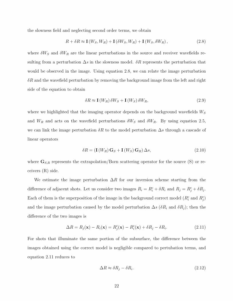
the slowness field and neglecting second order terms, we obtain
R + δR ≈ I (WS,WR) + I (δWS,WR) + I (WS, δWR) , (2.8)
where δWS and δWR are the linear perturbations in the source and receiver wavefields re-
sulting from a perturbation ∆s in the slowness model. δR represents the perturbation that
would be observed in the image. Using equation 2.8, we can relate the image perturbation
δR and the wavefield perturbation by removing the background image from the left and right
side of the equation to obtain
δR ≈ I (WR) δWS + I (WS) δWR, (2.9)
where we highlighted that the imaging operator depends on the background wavefields WS
and WR and acts on the wavefield perturbations δWS and δWR. By using equation 2.5,
we can link the image perturbation δR to the model perturbation ∆s through a cascade of
linear operators
δR = (I (WR) GS + I (WS) GR) ∆s, (2.10)
where GS,R represents the extrapolation/Born scattering operator for the source (S) or re-
ceivers (R) side.
We estimate the image perturbation ∆R for our inversion scheme starting from the
difference of adjacent shots. Let us consider two images Ri = Rci + δRi and Rj = Rc
j + δRj.
Each of them is the superposition of the image in the background correct model (Rci and Rc
j)
and the image perturbation caused by the model perturbation ∆s (δRi and δRj); then the
difference of the two images is
∆R = Rj(x)−Ri(x) = Rcj(x)−Rc
i (x) + δRj − δRi. (2.11)
For shots that illuminate the same portion of the subsurface, the difference between the
images obtained using the correct model is negligible compared to pertubation terms, and
equation 2.11 reduces to
∆R ≈ δRj − δRi. (2.12)
22

Equation 2.12 shows that under the assumption of small separation between the shots, the
image difference Rj(x) − Ri(x) gives us an approximation of the image perturbation we
need for the WEMVA operator. In operator notation, the estimated image perturbation is
obtained by applying the linear difference operator D to the migrated images
∆R ≈ D (Ri, Rj) . (2.13)
Finally, by combining equation 2.10, 2.12, and 2.13 we can link the image perturbation ∆R
to the model perturbation ∆s through a linear operator
∆R = L∆s, (2.14)
where L = D (I (WR) GS + I (WS) GR) is the cascade of the scattering operator GS,R that
relates the perturbation in the model ∆s to the perturbation in the wavefields δWS,R, the
imaging operator I that extracts the image from the wavefields, and the difference operator
in the shot domain D.
2.3.4 Workflow
We implement a nonlinear inversion scheme based on the solution of a sequence of lin-
earized problems. Each linearized problem is solved using a standard conjugate gradient
algorithm. Given a initial velocity model, we compute the associated migrated images for
a pair of adjacent shot-gathers. From the migrated images, we compute the displacement
vector field that warps one image into the image obtained from the adjacent shot. We
also compute the smooth image gradient for each migrated image. The smooth gradient
is the cascade of the ∇ operator and a low pass Gaussian filter to avoid the amplification
of high-frequency random noise. The dot product between the image gradient and the dis-
placement field associated with the relative shot gives the image perturbation that drives the
linearized migration velocity analysis algorithm. The linearized migration velocity analysis
procedure (Sava and Biondi, 2004) links the perturbation in the slowness model to the image
perturbation via a linear operator. The goal is to solve the system:
23

L∆s = ∆R, (2.15)
where the operator L and the image perturbation ∆R are defined in the previous sections.
We solve the linear problem using the conjugate gradient method. The solution of linear
problem is an estimate of the model perturbation. This perturbation is added to the current
model and we iterate the steps above until the stopping criterion is satisfied. The inter-
mediate model update modifies the operator L and thus allows us to solve the nonlinear
problem through a series of linearized approximations. For each linearized step, we perform
5 conjugate gradient iterations. The nonlinear inversion is performed by iterating until a
certain criterion is met: either the energy of the image perturbation ∆R falls below a certain
threshold or a maximum number of iterations is reached; in this paper, we fix the maximum
number of iterations.
2.4 Numerical Examples
Equation 2.3 shows that image-warping is an approximation of the image difference if we
assume that the warping vector field u is able to track the apparent displacement between
the two images. Nonetheless, the image perturbation obtained from image-warping depends
on only one image and is thus intrinsically more robust against cycle-skipping. We show
a comparison between the sensitivity kernels obtained by backprojecting the image pertur-
bation obtained from the forward WEMVA operator, from image-warping, and from image
difference, and demonstrate the superiority of image-warping. We apply our methodology
to two inversion tests. In the first one, we consider a simple model with a stack of horizontal
density interfaces in a vertical velocity gradient; the correct model is perturbed by two Gaus-
sian anomalies with opposite sign. We conclude the section showing the inversion results
obtained on the Marmousi dataset using a limited number of shot-gathers. Our methodology
is able to correct the model and obtain a more geologically plausible image.
24
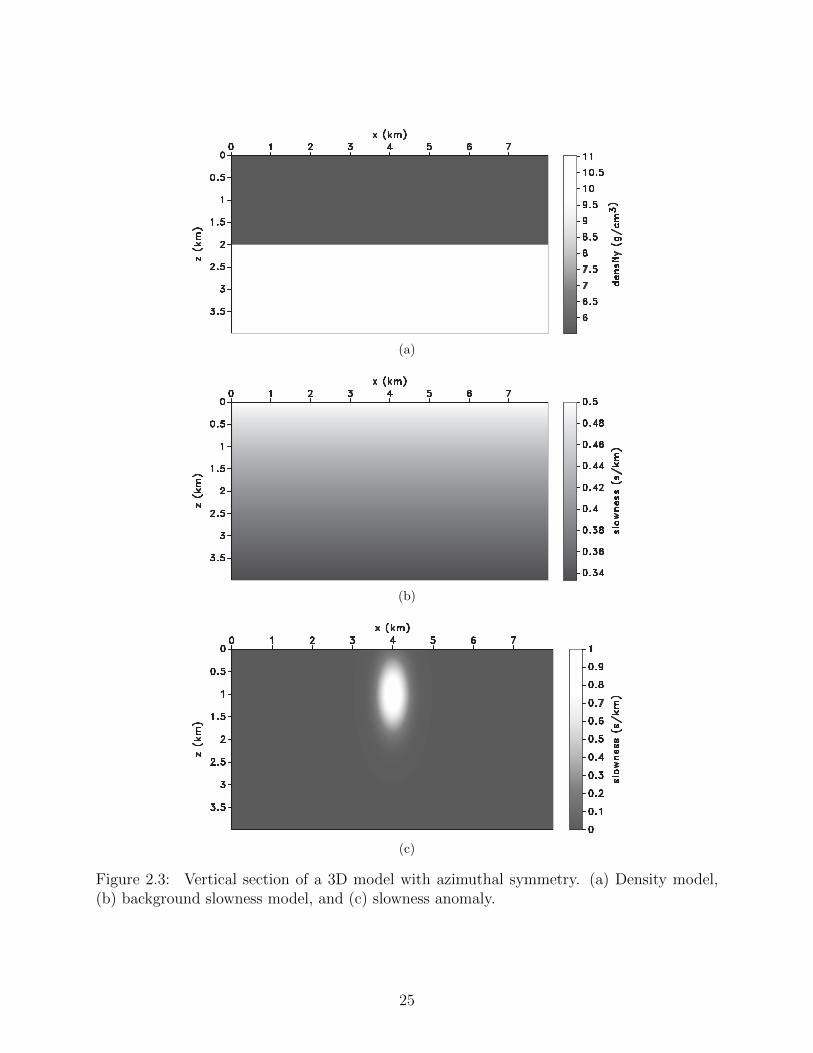
(a)
(b)
(c)
Figure 2.3: Vertical section of a 3D model with azimuthal symmetry. (a) Density model,(b) background slowness model, and (c) slowness anomaly.
25

(a) (b)
(c) (d)
(e) (f)
Figure 2.4: (a), (c), and (e) show the backprojection of image perturbations for a positivevalue of the anomaly in Figure 2.3(c). The image perturbations are obtained by forwardWEMVA operator, image-warping, and image difference respectively. (b), (d), and (f) showthe backprojections obtained for a negative anomaly. Image-warping consistently producessmoother backprojections that better approximate the ideal cases in (a) and (b). The oscilla-tions in the backprojections of image differences are connected with cycle-skipping problems.
26

2.4.1 Sensitivity to Cycle-Skipping and Backprojections
Let us consider the model in Figure 2.3. The reflecting interface in Figure 2.3(a) is
due to a density contrast. We model the data with a two-way finite-difference algorithm in
the vertical gradient of slowness in Figure 2.3(b). We migrate the data with a downward
continuation operator (Stoffa et al., 1990) and different amplitudes of the velocity anomaly
in Figure 2.3(c). We migrate two shots located at x = 2 km and x = 2.05 km for each
perturbation, compute the image perturbations using image difference and image-warping,
and compute the backprojections using the adjoint of the WEMVA operator. The columns of
Figure 2.4 show backprojection for different signs of the Gaussian anomaly; the left column
is the case of a fast anomaly, the left column is the case of a slow anomaly. The peak
value of the anomaly is ±0.5 km/s. The rows of Figure 2.4, from top to bottom, show the
backprojection in the ideal case, where the image perturbation is obtained from the forward
WEMVA operator, the backprojection obtained using the image perturbation computed
using image-warping, and finally the backprojection obtained using the image difference.
Observe that image-warping leads to smoother backprojections that better approximate the
ideal results. The highly oscillatory behavior of the backprojections obtained from image
difference is due to cycle skipping in the image domain. The warping vector field encodes the
shift between the two images, the image perturbation obtained by image-warping depends
on a single image and is thus immune from cycle skipping problems as long as the warping
vector field is accurately estimated.
The backprojections of the estimated image perturbations contain sidelobes, which have
been observed in other migration velocity analysis algorithms (Fei and Williamson, 2010);
we conjecture that these artifacts are attributable to the actual nonlinearity of the estimated
image perturbation with respect to the model parameters.
27

(a) (b)
Figure 2.5: Model for the inversion test: (a) stack of layers with alternating values of density(b) correct slowness model.
(a) (b)
Figure 2.6: Slowness model: (a) initial and (b) inverted after 13 nonlinear iterations.
28

2.4.2 Inversion Test
As mentioned before, the estimation of model parameters for wave phenomena is a non-
linear problem because the wave-equation is nonlinear in the model parameters (slowness,
density, etc.). In order to test our inversion methodology, we use custom implementation of a
nonlinear scheme based on the conjugate gradient algorithm (Vogel, 2002), in which the non-
linear problem is first linearized and an approximate solution is obtained. The approximate
solution is then used to obtain a new linearization and then a new approximate solution,
and so on. For every nonlinear iteration, we recompute the images and solve a linearized
problem assuming the new background medium. The model for the inversion is shown in
Figure 2.5: in Figure 2.5(a), the reflectors arise from density contrasts and, in Figure 2.5(b),
the correct slowness model is a simple vertical gradient. We consider 24 pairs of shots at the
surface; the receiver are evenly spaced by 20 m at each grid point at the surface. The shots
in each pair are 50 apart and the spacing between the pairs is 250 meters; the shot pairs do
not overlap.
The initial and updated velocity model are shown inFigure 2.6. The data for the inversion
test are computed through full-acoustic time-domain finite-difference modeling and Gaussian
random noise is added to each shot-gather separately. The signal-to-noise ratio is equal to
10. Absorbing boundary conditions are implemented to avoid surface-related multiples;
the internal multiples generated by the reflectors in the model are not subtracted from
the data and constitute additional source of noise. In the examples, the absolute value of
the peak of the velocity anomaly is 200 m/s, which is 10% of the minimum value of the
background velocity gradient. Nonetheless, the shape of the velocity anomaly causes severe
focusing/defocusing of the wavefield (depending on the sign of the anomaly), which makes
migration velocity analysis challenging, especially in the initial steps.
We run a nonlinear inversion involving five conjugate-gradient iterations for each lin-
earized step. We stop after 13 iterations, when the objective function starts oscillating,
which indicates we reached a minimum of the objective function. Figure 2.6 shows that
29
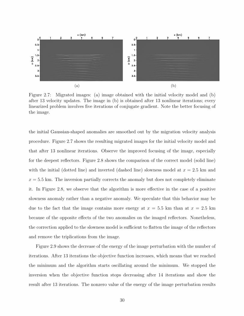
(a) (b)
Figure 2.7: Migrated images: (a) image obtained with the initial velocity model and (b)after 13 velocity updates. The image in (b) is obtained after 13 nonlinear iterations; everylinearized problem involves five iterations of conjugate gradient. Note the better focusing ofthe image.
the initial Gaussian-shaped anomalies are smoothed out by the migration velocity analysis
procedure. Figure 2.7 shows the resulting migrated images for the initial velocity model and
that after 13 nonlinear iterations. Observe the improved focusing of the image, especially
for the deepest reflectors. Figure 2.8 shows the comparison of the correct model (solid line)
with the initial (dotted line) and inverted (dashed line) slowness model at x = 2.5 km and
x = 5.5 km. The inversion partially corrects the anomaly but does not completely eliminate
it. In Figure 2.8, we observe that the algorithm is more effective in the case of a positive
slowness anomaly rather than a negative anomaly. We speculate that this behavior may be
due to the fact that the image contains more energy at x = 5.5 km than at x = 2.5 km
because of the opposite effects of the two anomalies on the imaged reflectors. Nonetheless,
the correction applied to the slowness model is sufficient to flatten the image of the reflectors
and remove the triplications from the image.
Figure 2.9 shows the decrease of the energy of the image perturbation with the number of
iterations. After 13 iterations the objective function increases, which means that we reached
the minimum and the algorithm starts oscillating around the minimum. We stopped the
inversion when the objective function stops decreasing after 14 iterations and show the
result after 13 iterations. The nonzero value of the energy of the image perturbation results
30

(a) (b)
Figure 2.8: Comparison of the initial (dotted line), inverted (dashed line), and exact (solidline) slowness model at (a) x = 2.5 km and (b) x = 5.5 km. The inversion reduces theanomaly but does not eliminate it. Nonetheless, the reflectors in Figure 2.7(b) are flattened.
Figure 2.9: The decrease of the energy of the image perturbation indicates that we areapproaching the correct model. We stopped the inversion after 13 iterations because theobjective function starts oscillating, which indicates that we reached a minimum of theobjective function.
31
from a number of factors: the random noise in the data, internal multiples, and the size
of the local window used to compute the dip and displacement field; all of them constrain
the accuracy, resolution, and sensitivity we can achieve. No regularization is implemented;
the footprint of the acquisition geometry is clearly visible in the inversion result, and it
represents an additional source of noise.
2.4.3 Local Marmousi Inversion
(a) (b)
Figure 2.10: Macro slowness model (a) for the Marmousi dataset and (b) slowness pertur-bation for the model in (a).
In this section, we consider a more complex synthetic example. Figure 2.10 shows the
correct macro velocity model for the Marmousi dataset and the anomaly used in the inversion
test. The model in Figure 2.10(a) is obtained by smoothing the exact Marmousi with a 15-
sample vertical and 30-sample horizontal triangular filter. We generate the data by single-
scattering Born finite-difference modeling; the reflectivity profile is the vertical derivative
of the exact Marmousi model. We want to show the ability of our method of recovering
model perturbation using a limited number of experiments (shots in this case); we consider
12 shots, evenly spaced by 0.04 km at the surface; the first shot is positioned at x = 0.96
km. The receivers are are spaced 0.008 km on the surface and they are located at every grid
point.
The anomaly is Gaussian-shaped with peak velocity 0.2 km/s and is subtracted from the
correct velocity field. The perturbation in slowness is obtained by converting to slowness
the correct and perturbed model and taking the difference of the former from the second.
32
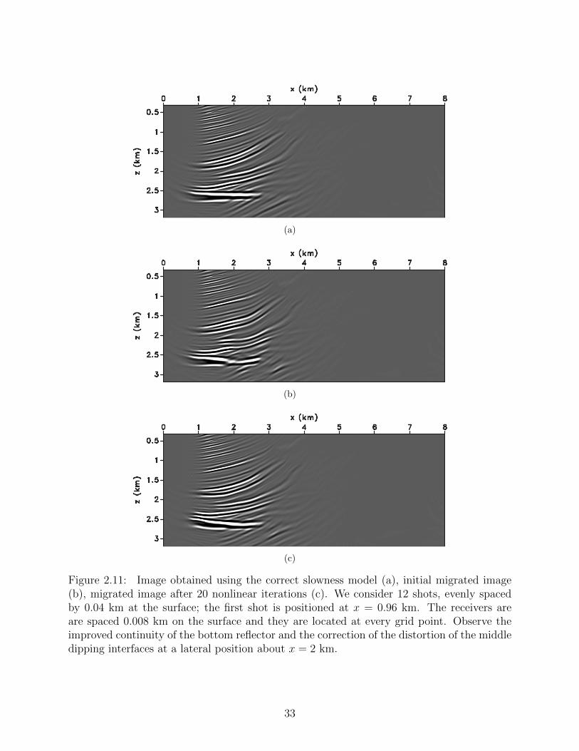
(a)
(b)
(c)
Figure 2.11: Image obtained using the correct slowness model (a), initial migrated image(b), migrated image after 20 nonlinear iterations (c). We consider 12 shots, evenly spacedby 0.04 km at the surface; the first shot is positioned at x = 0.96 km. The receivers areare spaced 0.008 km on the surface and they are located at every grid point. Observe theimproved continuity of the bottom reflector and the correction of the distortion of the middledipping interfaces at a lateral position about x = 2 km.
33
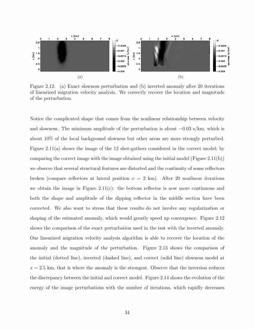
(a) (b)
Figure 2.12: (a) Exact slowness perturbation and (b) inverted anomaly after 20 iterationsof linearized migration velocity analysis. We correctly recover the location and magnitudeof the perturbation.
Notice the complicated shape that comes from the nonlinear relationship between velocity
and slowness. The minimum amplitude of the perturbation is about −0.03 s/km, which is
about 10% of the local background slowness but other areas are more strongly perturbed.
Figure 2.11(a) shows the image of the 12 shot-gathers considered in the correct model; by
comparing the correct image with the image obtained using the initial model (Figure 2.11(b))
we observe that several structural features are distorted and the continuity of some reflectors
broken (compare reflectors at lateral position x = 2 km). After 20 nonlinear iterations
we obtain the image in Figure 2.11(c): the bottom reflector is now more continuous and
both the shape and amplitude of the dipping reflector in the middle section have been
corrected. We also want to stress that these results do not involve any regularization or
shaping of the estimated anomaly, which would greatly speed up convergence. Figure 2.12
shows the comparison of the exact perturbation used in the test with the inverted anomaly.
Our linearized migration velocity analysis algorithm is able to recover the location of the
anomaly and the magnitude of the perturbation. Figure 2.13 shows the comparison of
the initial (dotted line), inverted (dashed line), and correct (solid line) slowness model at
x = 2.5 km, that is where the anomaly is the strongest. Observe that the inversion reduces
the discrepancy between the initial and correct model. Figure 2.14 shows the evolution of the
energy of the image perturbations with the number of iterations, which rapidly decreases
34

to 10% of the initial value and then flattens. We want to emphasize that we are able to
correct the anomaly in the model using a small number of shots despite the lack of full
illumination whereas methods based on focusing measures (i.e. migration velocity analysis
based on extended images) need complete angular coverage to evaluate focusing in the image
domain.
Figure 2.13: Comparison of the initial (dotted line), inverted (dashed line), and exact (solidline) slowness model at x = 2.5 km. Observe that inversion corrects the large discrepancybetween the initial and correct model.
35
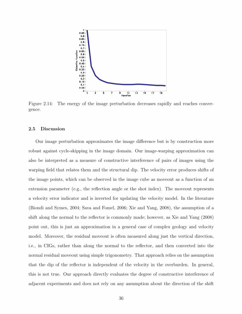
Figure 2.14: The energy of the image perturbation decreases rapidly and reaches conver-gence.
2.5 Discussion
Our image perturbation approximates the image difference but is by construction more
robust against cycle-skipping in the image domain. Our image-warping approximation can
also be interpreted as a measure of constructive interference of pairs of images using the
warping field that relates them and the structural dip. The velocity error produces shifts of
the image points, which can be observed in the image cube as moveout as a function of an
extension parameter (e.g., the reflection angle or the shot index). The moveout represents
a velocity error indicator and is inverted for updating the velocity model. In the literature
(Biondi and Symes, 2004; Sava and Fomel, 2006; Xie and Yang, 2008), the assumption of a
shift along the normal to the reflector is commonly made; however, as Xie and Yang (2008)
point out, this is just an approximation in a general case of complex geology and velocity
model. Moreover, the residual moveout is often measured along just the vertical direction,
i.e., in CIGs, rather than along the normal to the reflector, and then converted into the
normal residual moveout using simple trigonometry. That approach relies on the assumption
that the dip of the reflector is independent of the velocity in the overburden. In general,
this is not true. Our approach directly evaluates the degree of constructive interference of
adjacent experiments and does not rely on any assumption about the direction of the shift
36

of the image point in the migrated domain. Moreover, we are able to measure the 3D shift
of the image point between the two experiments and then capture the complete kinematic
information.
Migration velocity analysis is based on kinematic assumptions: the correct velocity model
returns a prestack image cube characterized by horizontal events along the experiment axis.
Note that we say horizontal and not constant in amplitude, highlighting the kinematic nature
of the conventional semblance principle. As already discussed by Mulder and Kroode (2002),
the amplitudes of images from nearby experiments are likely to be similar but not equal.
Reflection coefficients should be taken into account, and the velocity model itself, if it is
highly heterogeneous, can lead to important differences in the amplitudes.
The measure of velocity error is independent of the migration algorithm and in principle
either a one-way or a two-way velocity update engine can be used. The current implemen-
tation of the our WEMVA procedure relies on a one-way operator; the extension to two-way
operators is subject of ongoing research.
Compared to the data domain, the image domain is more robust but not immune from
cycle-skipping. If the current velocity model is reasonably close to the true model, a cy-
cle skip of the two images is unlikely. The chance of cycle skipping depends not only on
the velocity model but also on other factors such as the shot positions and the frequency
bandwidth of the signals. By increasing the distance between the shots, we violate the as-
sumption of sharing the same aperture and the potential for cycle skipping grows. Increasing
the bandwidth of the signals reduces the wavelength, thus further constraining the maxi-
mum distance between adjacent experiments. The shot distance enhances the the difference
between the apertures of the shots, thus the perturbation computed by image difference can
experience both cycle skipping and incomplete event cancellation, especially for strong and
shallow reflectors. The construction of the image perturbation as the first order term of a
Taylor series expansion removes the sensitivity to this source of cycle-skipping. Since the
warping vector field captures the information about the shift between the two images, our ap-
37
proach is intrinsically more robust against cycle-skipping. The correlation of two signals has
lower bandwidth than both the input signals: the spectrum of the correlation is equal to the
product of the spectra of the input signals. Image warping is based on local correlations; the
warping vector field is extracted by picking the maximum of the local correlations between
the input images. The shift information has by construction lower resolution with respect
to direct image difference. This lack of resolution gives our inversion algorithm robustness
against cycle-skipping away from the optimal solution but limits the amount of spatial de-
tails we can recover. The quick convergence in the both inversion tests and the inability to
perfectly flatten the horizontal reflectors in the first example describe the resolution limita-
tions of the method. Moreover, as Larner and Celis (2007) point out, the resolution power of
conventional semblance method comes from stacking over many experiments. Our approach
considers only two experiments at the time and is derived from differential semblance. Thus,
we observe the expected trade-off between robustness against cycle-skipping and resolution.
Finally, the shot-by-shot approach allows one to potentially bootstrap the MVA procedure
without first migrating the whole dataset; thus we can update the velocity model in an
iterative fashion with respect to shots. An iterative shot-based inversion has been already
proposed in the context of waveform inversion in the data-domain (see (Chauris and Plessix,
2012)); in this paper, we do not iteratively update the model for each consecutive pair of
experiments, we instead opt for a more traditional inversion procedure and combine the
partial updates from different pairs of shots into a global model update.
Several critical points must be carefully handled. First, since we are using only pairs of
experiments, the signal-to-noise ratio (SNR) can be low and the effectiveness of the algo-
rithm may be hampered by the quality of the data. The sensitivity to the signal-to-noise
ratio can be addressed using shot-encoding techniques (Morton and Ober, 1998; Perrone
and Sava, 2012a; Soubaras, 2006; Whitmore, 1995; Zhang et al., 2005) under the assumption
that the different experiments are contaminated by uncorrelated noise. Second, because of
cycle skipping between images, our approach can be ineffective if the shots are too far from
38

each other, the velocity model is very inaccurate, or the reflector geometry is complex (e.g.
around fault zones or in areas with conflicting dips). The similarity of nearby experiments is
an assumption of every DSO-like optimization scheme; if the particular acquisition geometry
or the complex wavepaths create shadow zones or illumination holes, DSO is likely to under
perform. Discrepancies in the images are due not only to velocity errors but also to the dif-
ferent set up of the two experiments; if the experiment sampling is coarse (e.g. distant shots
or plane waves that have very different ray-parameters), we need to guarantee that adjacent
experiments share the same aperture. The size of the local window used for computing the
image displacements should increase with decreasing depth to capture the apparent larger
separation closer to the shot positions. Two shots can be considered adjacent for a deep
reflector and not so for a shallow one, since the aperture of the image changes with depth. A
further remark is about the difference between 2D and 3D data: in 2D we can clearly specify
an order for the shots along a line, in 3D we cannot define a unique ordering since the shots
can be placed over a two-dimensional surface, and we do not address the possible strategies
to compare shots in a 3D acquisition in this paper. In the shot-domain, diving waves cre-
ate images that do not correspond to reflection events and that do not satisfy the warping
relationship assumed in this paper. Analogous considerations apply to multiply scattered
wave and converted waves, which are not correctly handled by migration algorithms based
on the Born approximation. Apparent reflectors associated with multiples and converted
waves do not satisfy the warping relationship we assumed for the definition of the image
perturbation and thus introduce a systematic bias in the inversion scheme. Also, in case of
highly refractive velocity models (Stolk and Symes, 2004), the kinematic artifacts created by
the imaging operator can severely affect the inversion, since they do not satisfy the criteria
we assume for defining our velocity error measure.
2.6 Conclusions
We introduce a new measure of velocity errors for migration velocity analysis in the
shot-domain. Our measure is based on an approximation of the difference between the
39
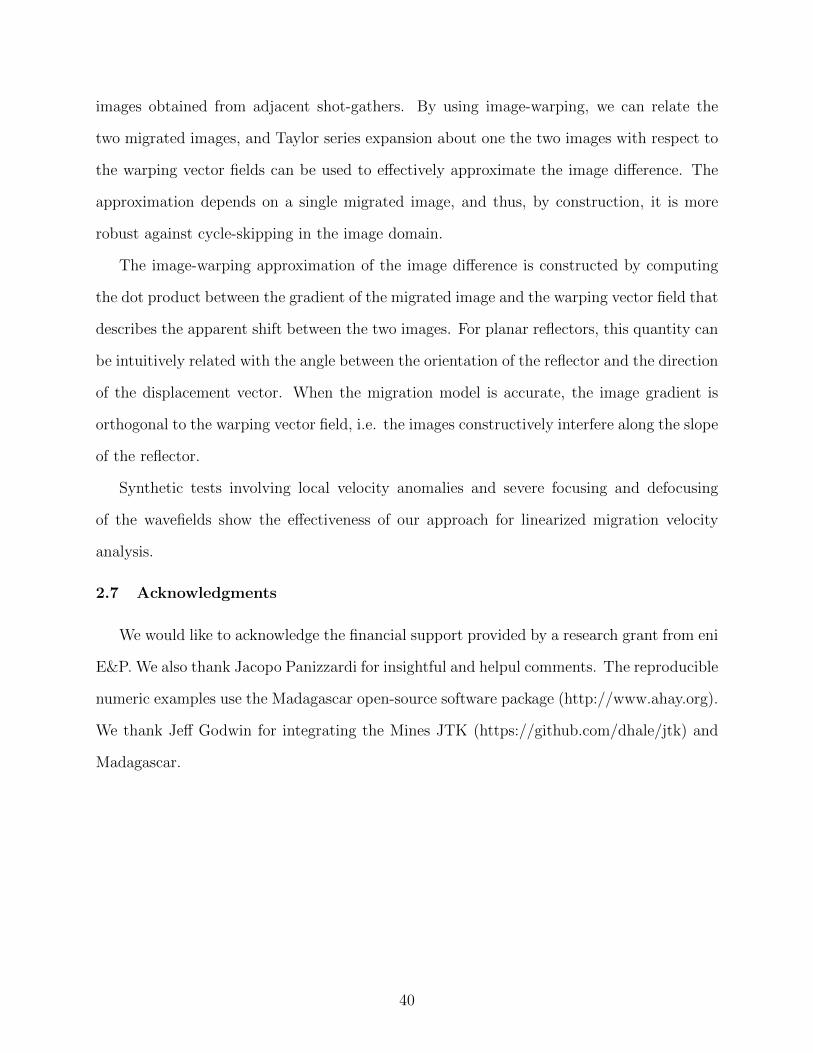
images obtained from adjacent shot-gathers. By using image-warping, we can relate the
two migrated images, and Taylor series expansion about one the two images with respect to
the warping vector fields can be used to effectively approximate the image difference. The
approximation depends on a single migrated image, and thus, by construction, it is more
robust against cycle-skipping in the image domain.
The image-warping approximation of the image difference is constructed by computing
the dot product between the gradient of the migrated image and the warping vector field that
describes the apparent shift between the two images. For planar reflectors, this quantity can
be intuitively related with the angle between the orientation of the reflector and the direction
of the displacement vector. When the migration model is accurate, the image gradient is
orthogonal to the warping vector field, i.e. the images constructively interfere along the slope
of the reflector.
Synthetic tests involving local velocity anomalies and severe focusing and defocusing
of the wavefields show the effectiveness of our approach for linearized migration velocity
analysis.
2.7 Acknowledgments
We would like to acknowledge the financial support provided by a research grant from eni
E&P. We also thank Jacopo Panizzardi for insightful and helpul comments. The reproducible
numeric examples use the Madagascar open-source software package (http://www.ahay.org).
We thank Jeff Godwin for integrating the Mines JTK (https://github.com/dhale/jtk) and
Madagascar.
40

CHAPTER 3
WAVEFIELD TOMOGRAPHY BASED ON LOCAL IMAGE CORRELATIONS
A paper submitted to Geophysical Prospecting
F. Perrone1, P. Sava1, and J. Panizzardi2
3.1 Summary
The estimation of a velocity model from seismic data is a crucial step for obtaining a high-
quality image of the subsurface. Velocity estimation is usually formulated as an optimization
problem where an objective function measures the mismatch between synthetic and recorded
wavefields and its gradient is used to update the model. The objective function can be defined
in the data-space (as in full-waveform inversion) or in the image-space (as in migration
velocity analysis). In general, the latter leads to smooth objective functions, which are
monomodal in a wider basin about the global minimum compared to the objective functions
defined in the data space. Nonetheless, migration velocity analysis requires construction of
common-image gathers at fixed spatial locations and subsampling of the image in order to
assess the consistency between the trial velocity model and the observed data. We present an
objective function that extracts the velocity error information directly in the image domain
without analyzing the information in common-image gathers. In order to include the full
complexity of the wavefield in the velocity estimation algorithm, we consider a two-way (as
opposed to one-way) wave operator, we do not linearize the imaging operator with respect
to the model parameters (as in linearized wave-equation migration velocity analysis), and
compute the gradient of the objective function using the adjoint-state method. We illustrate
our methodology with a few synthetic examples and test it on a real 2D marine streamer
dataset.
1Center for Wave Phenomena, Colorado School of Mines2Eni E & P
41

3.2 Introduction
Seismic imaging involves the estimation of wave propagation velocities in the subsurface
from seismic data recorded at the surface. Seismic velocities are related to other physical
parameters (for example, density and compressibility, which characterize the lithology of the
Earth), and rock-mechanics parameters (for example, porosity and fluid overpressure, which
are crucial in reservoir engineering) (Carcione, 2007).
Wave-equation tomography (Biondi and Sava, 1999; Tarantola, 1984; Woodward, 1992)
is a family of techniques that estimate the velocity model parameters from finite bandwidth
signals recorded at the surface. The inversion is usually formulated as an optimization
problem where the correct velocity model minimizes an objective function that measures the
inconsistency between a trial model and the observations. The objective function can be
defined either in the data-space (full-waveform inversion) or in the image-space (migration
velocity analysis).
Full-waveform inversion (FWI) (Pratt, 1999; Sirgue and Pratt, 2004; Tarantola, 1984)
addresses the estimation problem in the data-space and measures the mismatch between
the observations and simulated data. Full-waveform inversion reconstructs a model that
explains the data in the sense that the mismatch between acquired and simulated waveforms
is minimized. By matching both traveltimes and amplitudes, full-waveform inversion allows
one to achieve high-resolution (Sirgue et al., 2010). Nonetheless, a source estimate is needed,
the physics of wave propagation (for example, isotropic vs. anisotropic, acoustic vs. elastic,
etc.) must be correctly modelled, and a good parametrization (for example, impedance vs.
velocity contrasts) is crucial (Kelly et al., 2010). Moreover, an accurate initial model is key
to avoid cycle skipping and converge to the global minimum (instead of a local minimum)
of the objective function.
Because of the nonlinearity of the wavefields with respect to the velocity model, the
objective function in the data domain is highly multimodal (Santosa and Symes, 1989), and
local optimization methods can easily get trapped into local minima and fail to converge to
42

the correct model. This is particularly true for reflection full-waveform inversion. Refraction
full-waveform inversion focuses on diving waves and mutes the data, retaining only the diving
energy (Pratt, 1999). This leads to a better-behaved objective function but requires very
long offsets in order to record the refracted energy. Moreover, this approach limits the depth
at which a robust inversion result can be expected.
Migration velocity analysis (MVA) (Al-Yahya, 1989; Albertin et al., 2006; Biondi and
Sava, 1999; Chavent and Jacewitz, 1995; Faye and Jeannot, 1986; Fowler, 1985; Sava et al.,
2005) defines the objective function in the image space and is based on the semblance princi-
ple (Al-Yahya, 1989; Sattlegger, 1975). If the velocity model is correct, images from different
experiments must be consistent with each other because a single Earth model generates the
recorded data. A measure of consistency is usually computed through conventional semblance
(Taner and Koehler, 1969) or differential semblance (Symes, 1993; Symes and Carazzone,
1991). These two functionals analyze a set of migrated images at fixed locations in space;
they consider all the shots that illuminate the points under investigation. Migration ve-
locity analysis leads to smooth objective functions and well-behaved optimization problems
(Symes, 1991; Symes and Carazzone, 1991) and is less sensitive than full-waveform inversion
to the initial model. On the other hand, because we do not use amplitudes in the imaging
step, the estimated model has lower resolution than the ideal full-waveform inversion result
(Uwe Albertin, personal communication).
Migration velocity analysis measures either the invariance of the migrated images in
an auxiliary dimension (reflection angle, shot, etc.) (Al-Yahya, 1989; Rickett and Sava,
2002; Sava and Fomel, 2003; Xie and Yang, 2008) or focusing in an extended space (Rickett
and Sava, 2002; Sava and Vasconcelos, 2009; Symes, 2008; Yang and Sava, 2011b). All
these approaches require the migration of the entire survey in order to analyze the moveout
curve in common-image gathers or measure focusing at a specific spatial location. The
dimensionality of the (extended) image space and computational complexity of the velocity
analysis step rapidly explodes for realistic case scenarios. Moreover, because of the high
43
memory requirement for storing the partial information from each experiment, only a subset
of the image points can be considered in the evaluation of the objective function. Illumination
holes and/or irregular acquisition geometries can also impact the quality of the common-
image gathers but no systematic study of this problem is reported in the literature to our
knowledge.
Reverse-time migration (Baysal et al., 1983; McMechan, 1983) is routinely used in explo-
ration geophysics because of its ability to correctly handle the full complexity of the wave
propagation phenomena (under the assumption that the physics of wave propagation in the
subsurface is correctly modeled). Its computational cost is nevertheless still prohibitive and
limits its integration into a migration velocity analysis loop that requires the extraction of
common-image gathers for moveout analysis. A migration velocity analysis procedure based
on a full-wave propagation engine allows exploitation of more complex wave phenomena
(e.g. overturning reflection, prismatic waves, and multiples) and increases the amount of
information in the data that can be used (Farmer et al., 2006).
Reverse-time migration works only in common-shot and common-receiver configurations,
so the choice of the shot-domain for performing migration velocity analysis with a two-way en-
gine may be preferable. Here, we use the word “shot” in its broader sense to include synthetic
shot-gathers like plane-wave sources (Liu et al., 2006; Stoffa et al., 2006; Whitmore, 1995;
Zhang et al., 2005), random shot-encoded sources (Morton and Ober, 1998; Romero et al.,
2000) or any other phase-/amplitude-encoded source (Perrone and Sava, 2012a; Soubaras,
2006) in the range of shot-profile migration. Reverse-time migration automatically and
without additional costs outputs shot-domain common-image gathers; unfortunately, the
migrated-shot domain is notoriously not optimal for velocity estimation because of migra-
tion artifacts (Stolk and Symes, 2004) and noisy common-image gathers (Zhang et al., 2010).
Even when the velocity model is correct, the reflection events in shot-domain image gathers
are very noisy and semblance is challenging to evaluate. Previously proposed techniques in
the shot-domain consider all shots in the survey, thus exploiting the power of stacking to
44

attenuate the effects of noise and artifacts in the common-image gathers (Al-Yahya, 1989;
Chavent and Jacewitz, 1995; de Vries and Berkhout, 1984; Xie and Yang, 2008; Yilmaz and
Chambers, 1984).
We propose an objective function that evaluates the degree of semblance between images
through local correlations in the image space and does not require to pick moveout or evaluate
focusing in common-image gathers (CIGs). We use the morphologic relationship between
images from nearby experiments to define an objective function that measures shifts in the
image space (Perrone and Sava, 2012c). The methodology described in this work takes
advantage of the local coherency of the migrated reflectors in the image domain to overcome
the limitations of shot-domain CIGs. We compute the gradient of the objective function
with the adjoint-state method (Plessix, 2006). Our approach does not require to store
partial information about common-image gathers and avoids the need to pick moveout on
gathers, and allows us to include all points illuminated by the seismic experiments in the
velocity model building.
3.3 Theory
We define a measure of velocity error, r (x), where x = (z, x), in the image domain using
penalized local correlation that measure the apparent shifts between single shots migrated
images. We define the objective function of the optimization problem as the energy (l2
norm) of r (x). Other norms (l1, Huber norm, hybrid, etc.) can be used to promote sparsity
and gain robustness against non-Gaussian noise in the data (Brossier et al., 2010). We use
adjoint-state calculations to compute the gradient of the objective function.
3.3.1 Image Correlation Objective Function
There are at least two options for measuring similarity between two images. We can
compute the point-wise difference function is
r (x) = Ri+1 (x)−Ri (x) , (3.1)
45

where Ri (x) and Ri+1 (x) are the migrated images for ith and (i + 1)th shot, respectively.
The two shots are assumed to be close and to image the same area in the subsurface. Plessix
(2006) and Symes (1993) use the energy of the image difference as a regularization term
for full-waveform inversion and not as a stand-alone objective function. Notice that if the
velocity model used in migration is severely inaccurate, we can have cycle skipping in the
image space or, in other words, the difference between the two images can produce two
events if the position of the same reflector in the two images changes more than a quarter
of a wavelength. This problem is analogous to what happens in full-waveform inversion in
the data space.
An alternative solution is to restate the semblance principle as follows: if the velocity
model is correct, two images from nearby experiments construct the final image along the
direction of the reflectors (Perrone and Sava, 2012c). This is equivalent to the standard
assumption that, if the model is correct, the prestack image-cube is invariant with respect
to the shot position, i.e., no moveout in the shot-domain common-image gathers (Xie and
Yang, 2008).
The structural dip is an attribute that is commonly extracted in seismic processing
(Fomel, 2002; van Vliet and Verbeek, 1995). The similarity of two images perpendicular
to the structural dip can be measured by means of penalized local correlations (Perrone and
Sava, 2012c). We illustrate this idea on a simple model with a single horizontal density
interface; the correct velocity model is constant and equal to 2.0 km/s. Figure 3.1 shows
the dip and apparent displacement vector field (solid and dashed arrows, respectively) at
particular spatial locations. Observe that the two vectors are orthogonal when the velocity
model is correct.
The computation of the displacement field requires a highly nonlinear procedure, which
extracts the maximum of the local correlations at every image point (Hale et al., 2008). We
reformulate the problem of evaluating the orthogonality between dip and displacement using
local correlations between images Ri (x) and Ri+1 (x) (Hale, 2006)
46
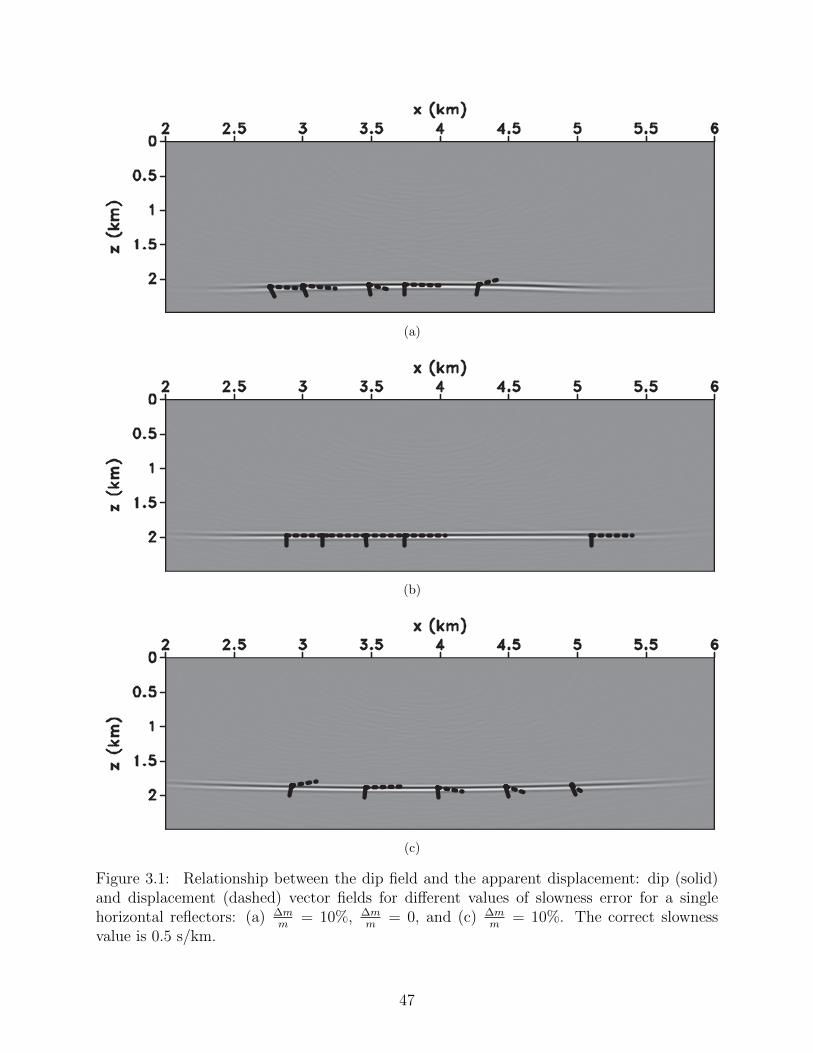
(a)
(b)
(c)
Figure 3.1: Relationship between the dip field and the apparent displacement: dip (solid)and displacement (dashed) vector fields for different values of slowness error for a singlehorizontal reflectors: (a) ∆m
m= 10%, ∆m
m= 0, and (c) ∆m
m= 10%. The correct slowness
value is 0.5 s/km.
47
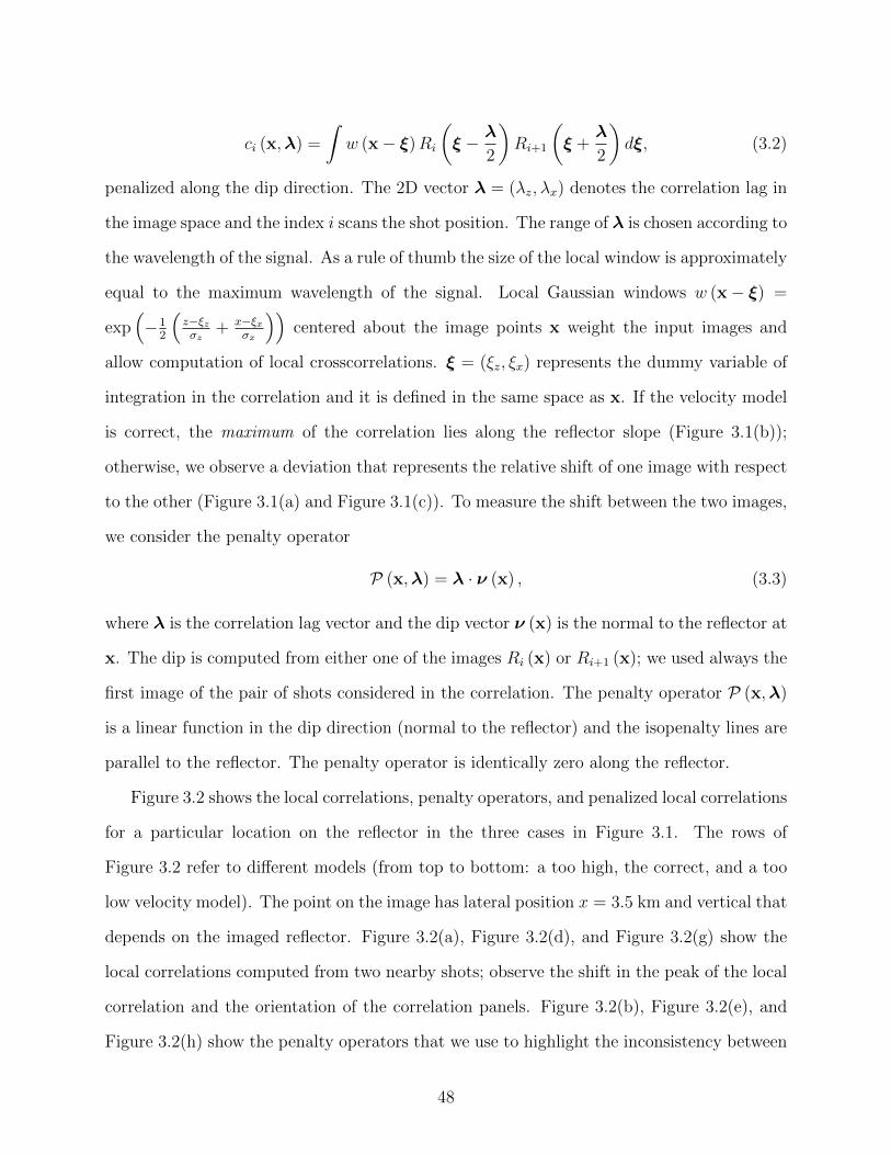
ci (x,λ) =
∫w (x− ξ)Ri
(ξ − λ
2
)Ri+1
(ξ +
λ
2
)dξ, (3.2)
penalized along the dip direction. The 2D vector λ = (λz, λx) denotes the correlation lag in
the image space and the index i scans the shot position. The range of λ is chosen according to
the wavelength of the signal. As a rule of thumb the size of the local window is approximately
equal to the maximum wavelength of the signal. Local Gaussian windows w (x− ξ) =
exp(−1
2
(z−ξzσz
+ x−ξxσx
))centered about the image points x weight the input images and
allow computation of local crosscorrelations. ξ = (ξz, ξx) represents the dummy variable of
integration in the correlation and it is defined in the same space as x. If the velocity model
is correct, the maximum of the correlation lies along the reflector slope (Figure 3.1(b));
otherwise, we observe a deviation that represents the relative shift of one image with respect
to the other (Figure 3.1(a) and Figure 3.1(c)). To measure the shift between the two images,
we consider the penalty operator
P (x,λ) = λ · ν (x) , (3.3)
where λ is the correlation lag vector and the dip vector ν (x) is the normal to the reflector at
x. The dip is computed from either one of the images Ri (x) or Ri+1 (x); we used always the
first image of the pair of shots considered in the correlation. The penalty operator P (x,λ)
is a linear function in the dip direction (normal to the reflector) and the isopenalty lines are
parallel to the reflector. The penalty operator is identically zero along the reflector.
Figure 3.2 shows the local correlations, penalty operators, and penalized local correlations
for a particular location on the reflector in the three cases in Figure 3.1. The rows of
Figure 3.2 refer to different models (from top to bottom: a too high, the correct, and a too
low velocity model). The point on the image has lateral position x = 3.5 km and vertical that
depends on the imaged reflector. Figure 3.2(a), Figure 3.2(d), and Figure 3.2(g) show the
local correlations computed from two nearby shots; observe the shift in the peak of the local
correlation and the orientation of the correlation panels. Figure 3.2(b), Figure 3.2(e), and
Figure 3.2(h) show the penalty operators that we use to highlight the inconsistency between
48

(a) (b) (c)
(d) (e) (f)
(g) (h) (i)
Figure 3.2: Measure of the relative displacement between two images using penalized localcorrelations. We consider 2 images from nearby experiments of the reflector in Figure 3.1;each row (from top to bottom) represents a different model: too high, correct, and too low;the columns show (from left to right) the local correlation panel, the penalty operator used,and the penalized local correlation. For each model, we pick a point on the reflector withlateral coordinate x = 3.5 km. The vertical coordinate changes as a function of model pa-rameters because the depth of the reflector changes. Observe the asymmetry of the penalizedlocal correlations for the wrong models: the mean value (i.e., the stack over the correlationlags) of the penalized correlations gives us a measure of the relative shift between two images.
49

the dip measured on the image and the local correlations. The orientation of the penalty
operators does indeed depend on the measured dip. We applied a Gaussian taper to the
penalty operator in order to have a smooth transition to zero along the sides of the penalty
operator panel and thus remove possible artifacts due to abrupt truncations. Figure 3.2(c),
Figure 3.2(f), and Figure 3.2(i) show the penalized correlations. The apparent shift is now
clear as a sign unbalance in the panels. When the velocity model is correct, the penalized
correlation is an odd function (i.e., zero mean value) (Figure 3.2(f)); on the other hand,
the panels lose their symmetry when the model is incorrect (Figure 3.2(c)and Figure 3.2(i)).
The sign of the mean value of the penalized panels measures the apparent shift between the
two images.
We define the velocity error measure as the average value of the local correlations ci (x,λ)
penalized by the penalty operator P (x,λ):
ri (x) =
∫P (x,λ) ci (x,λ) dλ. (3.4)
This quantity measures the relative shift of one image with respect to the other directly in
the image space and can be used for velocity analysis.
The shifts r (x) in equation 3.4 are computed from the migrated images Ri (x) and
Ri+1 (x). The dependency on the source and receiver wavefields, and then the velocity
model, is hidden in the imaging condition we use to construct the migrated image. An
image of the subsurface R (x) is conventionally computed as the zero-lag time correlation of
the source and receiver wavefields (Claerbout, 1985):
R (x) =
∫T
us (x, t)ur (x, t) dτ, (3.5)
where T is the recording time interval in the data.
We define the objective function
J (m) =1
2
∑i
∥∥∥∥∫ P (x,λ) ci (x,λ) dλ
∥∥∥∥2
x
, (3.6)
50

where m represents the model parameters. Figure 3.3 shows the values of the objective
function for different constant perturbations of the model used for the simple example shown
in Figure 3.1. The objective function is smooth and convex in the range of errors considered.
Figure 3.3: Values of the objective function for different errors in the slowness model. Weconsider constant perturbations ranging from −10% to 10% of the exact value (0.5 s/km).
3.3.2 Computation of the Gradient with the Adjoint-State Method
Because of the dimensionality of the model, the optimization problem is addressed using a
local gradient-based method (steepest descent, conjugate gradient, etc.) (Vogel, 2002). The
computation of the derivative of the state variables with respect to the model parameters
(Frechet derivatives) is not practical (or even possible) because of the large number of dimen-
sions of the model space. The adjoint-state method (Lions, 1972; Plessix, 2006) is an efficient
algorithm that computes the gradient of an objective function, which depends on some vari-
ables that describe the state of the physical system under analysis (state variables), without
computing the Frechet derivatives of these variables with respect to the model parameters.
The adjoint-state method consists of four steps: the computation of the state variables,
the computation of the adjoint sources, the computation of the adjoint-state variables, and
finally the computation of the gradient of the objective function. The first and third step (the
evaluation of the state and adjoint-state variables) require the solution of the wave-equation
51
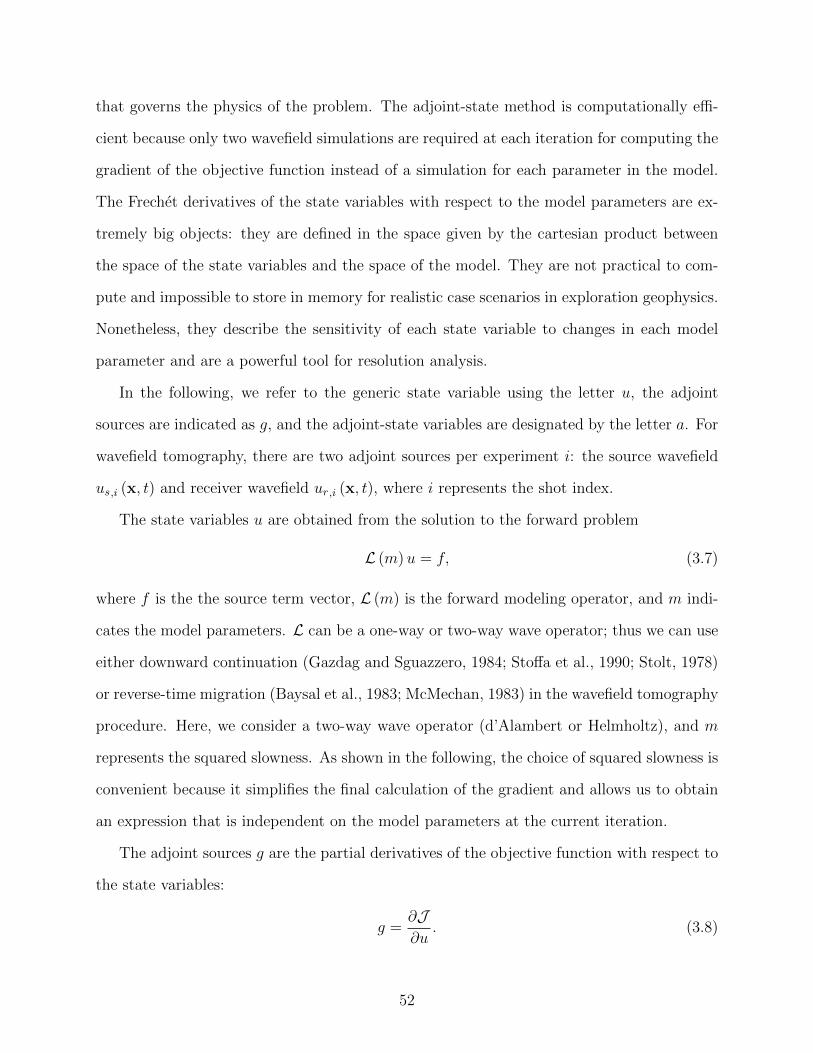
that governs the physics of the problem. The adjoint-state method is computationally effi-
cient because only two wavefield simulations are required at each iteration for computing the
gradient of the objective function instead of a simulation for each parameter in the model.
The Frechet derivatives of the state variables with respect to the model parameters are ex-
tremely big objects: they are defined in the space given by the cartesian product between
the space of the state variables and the space of the model. They are not practical to com-
pute and impossible to store in memory for realistic case scenarios in exploration geophysics.
Nonetheless, they describe the sensitivity of each state variable to changes in each model
parameter and are a powerful tool for resolution analysis.
In the following, we refer to the generic state variable using the letter u, the adjoint
sources are indicated as g, and the adjoint-state variables are designated by the letter a. For
wavefield tomography, there are two adjoint sources per experiment i: the source wavefield
us,i (x, t) and receiver wavefield ur,i (x, t), where i represents the shot index.
The state variables u are obtained from the solution to the forward problem
L (m)u = f, (3.7)
where f is the the source term vector, L (m) is the forward modeling operator, and m indi-
cates the model parameters. L can be a one-way or two-way wave operator; thus we can use
either downward continuation (Gazdag and Sguazzero, 1984; Stoffa et al., 1990; Stolt, 1978)
or reverse-time migration (Baysal et al., 1983; McMechan, 1983) in the wavefield tomography
procedure. Here, we consider a two-way wave operator (d’Alambert or Helmholtz), and m
represents the squared slowness. As shown in the following, the choice of squared slowness is
convenient because it simplifies the final calculation of the gradient and allows us to obtain
an expression that is independent on the model parameters at the current iteration.
The adjoint sources g are the partial derivatives of the objective function with respect to
the state variables:
g =∂J∂u
. (3.8)
52

The actual expression of the adjoint sources depends on the objective function. The par-
ticular design of the objective function impacts the adjoint sources and characterizes the
particular wavefield tomography strategy proposed. In the following sections, we derive the
expressions for the adjoint sources for an objective function based on local image correlations
(equation 3.6).
We solve the adjoint problem and compute the adjoint variables a using the adjoint
sources g as the force term:
L∗ (m) a = g, (3.9)
where L∗ (m) is the operator adjoint to L (m). Finally, the gradient is given by the inner
product
∂J∂m
= −⟨a,∂L∂m
⟩. (3.10)
For example, for the Helmholz operator parametrized in terms of slowness squared, L =
−∇2 − mω2, the partial derivative ∂L∂m
returns a simple scaling factor −ω2, and the inner
product 〈a, ∂L∂m〉 = −ω2〈a, u〉 can also be seen as the scaled zero-lag correlation of u and a,
similar to the procedure employed in conventional FWI.
3.3.3 Adjoint Sources
As described in the previous section, the adjoint sources g = ∂J∂u
are the derivatives of the
objective function with respect to the state variables. In our objective function, we consider
the dip field a slowly varying function of state variables and neglect the derivative of the
penalty operator with respect to u. The details of the derivation of the expressions for the
adjoint sources are in appendix A; here, we report the final result:
gs,i = ur,i (η, t)
[ri−1
∫P (x,λ)w
(x− η +
λ
2
)Ri−1 (η − λ) dλ
+ ri
∫P (x,λ)w
(x− η − λ
2
)Ri+1 (η + λ) dλ
], (3.11)
53
and
gr,i = us,i (η, t)
[ri−1
∫P (x,λ)w
(x− η +
λ
2
)Ri−1 (η − λ) dλ
+ ri
∫P (x,λ)w
(x− η − λ
2
)Ri+1 (η + λ) dλ
], (3.12)
where gs,i = gs,i (x,η, t) and gr,i = gr,i (x,η, t) indicate the adjoint sources for the source and
receiver wavefield of the ith shot, respectively, and ri = ri (x) is defined as in equation 3.4.
Notice that the adjoint sources depend on 3 variables (x,η, t). The vector x represents
the physical space, where model and image are defined; the variable t identifies the time axis;
η is an auxiliary vector defined in the physical space that spans the local window around
every image point. The adjoint source is obtained by spreading the value of the shift at each
point in a window around the image point and by weighting it by the the integral over λ,
which represents a local convolution of the image and the penalty operator. The value of
r (x) in equation 3.4 measures the relative displacement of one image with respect to the
other; the adjoint source thus estimates the curvature of the moveout in the shot-domain
common-image gathers at each image point and scales the background wavefields by this
value.
In 3D, Equations 3.11 and 3.12 remain valid but all the quantites involved are defined
in a 3D space. The main difference between the two- and three-dimensional case is the
computation of the r (x) and the ordering of the shots. In 2D there exists a clear ordering
(along the line) for the seismic experiments, whereas in 3D every shot can have a number of
neighboring experiments.
The dependence of the penalty operator P (x,λ) on the state variables u passes through
the definition of the dip vector ν (x), which is normal to the reflectors at every point in the
image. The dip field defines the wavefront set of the function that represents the reflection
events in the image (Chang et al., 1987); the link between the image (and the wavefields)
and the dip field can be written exploiting the concept of gradient-squared tensor (van Vliet
54

and Verbeek, 1995): the dip vector is the eigenvector associated with the largest eigenvalues.
There is no simple linear relationship between the dip vector and the wavefields, i.e. the state
variables. Neglecting this term in the computation of the adjoint sources may introduce an
error of the same order of magnitude of the term considered. A thorough study of ∂P/∂u and
its impact on the computation of both the adjoint sources and the gradient of the objective
function is subject for future research.
3.3.4 Flat Reflector in a Constant Velocity Medium
Figure 3.1 shows the migrated images of a horizontal interface obtained from a shot
located at x = 4 km. The data are computed in a constant 2.0 km/s velocity medium
using a two-way finite-difference scheme. We migrate the data with three different slowness
models and perform sensitivity analysis for our methodology. Observe that with a single
shot, the image of a horizontal reflector curves up or down depending on the sign of the
velocity error. The relative displacement between different images is measured by the value
of r (x) defined in equation 3.4. Figure 3.4 shows the shifts calculated using two images from
adjacent shots. Observe the change in sign across the zero-offset reflection point and how
the sign changes with the velocity error. Note also the effect of limited aperture on the shift
estimation: the abrupt change in the estimated shift at the edges of the reflector is due to
uneven illumination from the three experiments.
In Figure 3.5, we show the gradient computed from the correlation objective function.
We consider three shots to compute r (x) and use only the wavefields of the central exper-
iment to compute the gradient. We also focus our attention in the portion of the reflector
that is illuminated by all three shots in order to avoid artifacts due to the erroneous shift
estimation at the edge of the reflector. The gradient of the objective function represents
the direction of maximum increase of the function itself and its sign depends on the chosen
parametrization. We compute the gradient with respect to slowness squared; this means that
a positive gradient points toward slower models whereas a negative gradient points toward
faster models.
55

(a)
(b)
(c)
Figure 3.4: For the three cases in Figure 3.1, we compute the shifts r (x) according toequation 3.4. The sign of the shifts indicates the relative displacement of one image withrespect to the other.
56
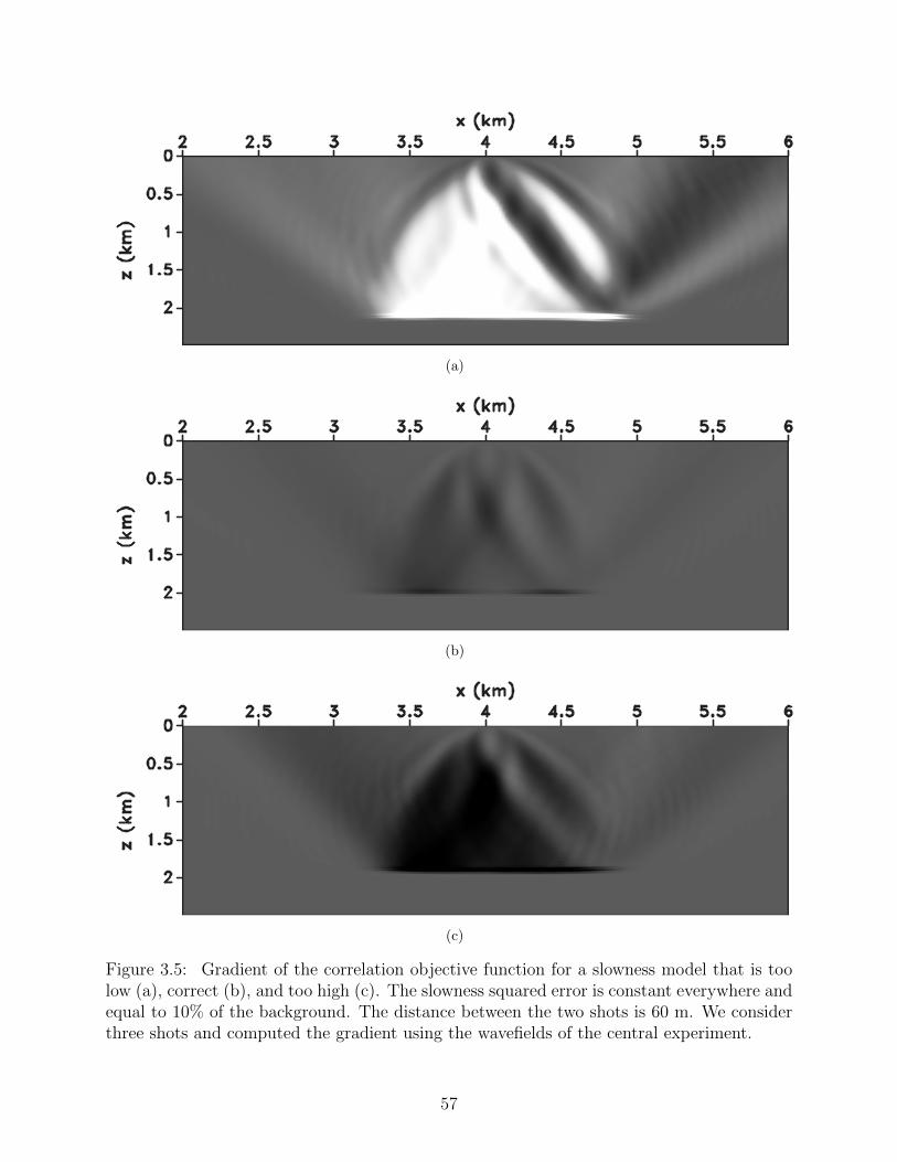
(a)
(b)
(c)
Figure 3.5: Gradient of the correlation objective function for a slowness model that is toolow (a), correct (b), and too high (c). The slowness squared error is constant everywhere andequal to 10% of the background. The distance between the two shots is 60 m. We considerthree shots and computed the gradient using the wavefields of the central experiment.
57

3.4 Examples
We show the results of our inversion methodology using two datasets. First, we run
an inversion test on a simple synthetic heterogeneous model with different layers using 40
shots evenly spaced 200 m apart and receivers at every grid point on the surface. We use
shot-domain common-image gathers to assess the quality of the result and to show that our
methodology is able to obtain a set of images that is invariant with respect to the experiment
position. Second, we apply our methodology to a real 2D marine dataset. We invert 200
shot-gathers acquired with a streamer cable. Each shot includes 99 receivers. The shot and
receiver sampling is 12.5 meters and the maximum offset is 1.225 km.
3.4.1 Synthetic Laterally Heterogeneous Model
Figure 3.6: Velocity model used to generate the full-acoustic data. Absorbing boundaryconditions have been applied at all sides of the model. The lighter shades of grey indicatefaster layers. The top layer has velocity of water (1.5 km/s).
We use the synthetic heterogeneous model in Figure 3.6 to test our inversion algorithm.
The model has a few layers with different dips and a syncline structure with an inversion in
the otherwise decreasing slowness trend. We generate full-acoustic (i.e., non-Born) data with
absorbing boundary conditions (no free-surface multiples) and random Gaussian noise with
58

(a)
(b)
(c)
Figure 3.7: Initial velocity model (a), associated migrated image (b), and shot-domaincommon-image gathers. The reflectors are severely defocused and mispositioned. Observethe curvature of the common-image gathers that shows how different experiments image thereflectors at different depths.
59

a signal-to-noise ratio of 10. We model 40 shots evenly spaced 200 m apart with receivers
at every grid point on the surface. We heavily smooth the initial model in Figure 3.6 and
obtain the initial velocity model for migration (Figure 3.7(a)). The source signal is a Ricker
wavelet with peak frequency 15 Hz. The modelled data are then bandpass filtered in order
to limit the maximum frequency to 25 Hz. Figure 3.7(b) shows the stack of the migrated
images obtained from the initial model; if we compare the correct model in Figure 3.6 and the
migrated image we can observe the mispositioning of the reflecting interfaces. We construct
10 shot-domain common image gathers to assess the overall focusing of the image. These
gathers are simply the juxtaposition of the migrated images at fixed lateral positions (from
x = 0 km to x = 9 km every 1 km). Figure 3.7(c) shows such gathers for the initial
model: the position of the reflectors changes as a function of experiment (the images do
not satisfy the semblance principle) and the model is thus not accurate. After 13 waveform
tomography steps, we recover the model in Figure 3.8(a). The model is still quite smooth,
but the migrated image shows a noticeable improvement in the position of the reflectors
(Figure 3.8(b)), and the shot-domain common-image gathers in Figure 3.8(c) clearly indicate
better focusing. Moreover, the imaged reflectivity is now consistent with the actual slowness
contrasts in the exact model; observe the change in polarity of the reflector at z = 3 km
between the initial and final image, that corresponds to a decrease in velocity. We impose
conformity between the model update and the layers in the image by means of a structure-
oriented smoothing operator, which steers the gradient of the objective function by smoothing
along the reflector slope. We used the complete stacked image to guide the smoothing of
the gradient. This approach is conceptually similar to the sparse inversion proposed by Ma
et al. (2010). Figure 3.9 shows the evolution of the objective function with iterations. Notice
the monotonic decrease in the value of the residual and the flattening when the algorithm
converges. The algorithm stops when the objective function changes less than 1% of the
initial value over three consecutive iterations. The inversion shows a rapid convergence
in the very first iterations of steepest-descent: the structure-oriented smoothing forces the
60
gradient to conform to the geometry of the layers and speeds up convergence to an acceptable
model.
3.4.2 Real Data
We test our inversion algorithm on a real dataset supplied by eni E&P. The data consists
of a single 2D line, the total number of shots is 3661, the streamer has 99 receivers, and the
maximum offset is 1.225 km. The data have been regularized and demultipled. Source and
receiver spacing is equal to 12.5 m. We show a subset of the entire dataset; we downsample
the shots 2 : 1 and analyze 200 shots. The first shot location is x = 11.25 km. The frequency
content of the data ranges between 3 and 75 Hz.
We fix the water velocity to 1.51 km/s and start inversion from a slowness vertical
gradient (Figure 3.10(a)). The migrated image using the initial velocity model is shown in
Figure 3.10(b).
Observe the partial overlap between different events because of the moveout in the image-
gathers. The interference between moveout curves that are relative to different reflection
events would cause a naive MVA approach, as the total stack power maximization, to cycle
skip and not converge.
The inversion converges after 90 iterations of steepest descent and returns the model in
Figure 3.11(a); the associated migrated image is shown in Figure 3.10(b). The migrated
images reconstructed with the initial and final model are displayed using the same scale.
In order to better understand the error in the velocity model, we show the shot-domain
CIGs at 4 different locations (Figure 3.12(a)-Figure 3.12(d)). The CIGs are extracted every
kilometer from x = 12 km. The stong moveout function of the shot position indicates error
in the velocity model. Observe the increased strength of the reflectors after inversion. The
common-image gathers in Figure 3.12(e)-Figure 3.12(h) show that the single migrated images
locate reflectors at consistent depths (in agreement with the semblance principle) and thus
the velocity model is kinematically accurate.
61

(a)
(b)
(c)
Figure 3.8: Velocity model after 15 iterations of waveform inversion (a), migrated image (b),and shot-domain common-image gathers (c). Observe the improved focusing and positioningof the reflectors. The common-image gathers show that the images are invariant in the shotdirection and the model is thus kinematically correct. Observe the profile of the variouslayers in the reconstructed model.
62
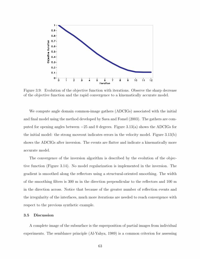
Figure 3.9: Evolution of the objective function with iterations. Observe the sharp decreaseof the objective function and the rapid convergence to a kinematically accurate model.
We compute angle domain common-image gathers (ADCIGs) associated with the initial
and final model using the method developed by Sava and Fomel (2003). The gathers are com-
puted for opening angles between −25 and 0 degrees. Figure 3.13(a) shows the ADCIGs for
the initial model: the strong moveout indicates errors in the velocity model. Figure 3.13(b)
shows the ADCIGs after inversion. The events are flatter and indicate a kinematically more
accurate model.
The convergence of the inversion algorithm is described by the evolution of the objec-
tive function (Figure 3.14). No model regularization is implemented in the inversion. The
gradient is smoothed along the reflectors using a structural-oriented smoothing. The width
of the smoothing filters is 300 m in the direction perpendicular to the reflectors and 100 m
in the direction across. Notice that because of the greater number of reflection events and
the irregularity of the interfaces, much more iterations are needed to reach convergence with
respect to the previous synthetic example.
3.5 Discussion
A complete image of the subsurface is the superposition of partial images from individual
experiments. The semblance principle (Al-Yahya, 1989) is a common criterion for assessing
63

(a)
(b)
Figure 3.10: Initial migration model and migrated image.
64
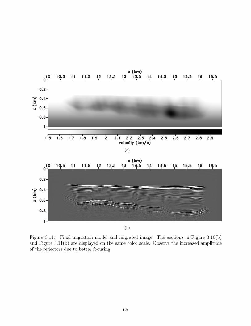
(a)
(b)
Figure 3.11: Final migration model and migrated image. The sections in Figure 3.10(b)and Figure 3.11(b) are displayed on the same color scale. Observe the increased amplitudeof the reflectors due to better focusing.
65

(a) (b) (c) (d)
(e) (f) (g) (h)
Figure 3.12: Shot-domain CIGs computed for the incorrect model at (a) x = 12 km, (b)x = 13 km, (c) x = 14 km, and (d) x = 15 km, and gathers computed after inversion at thesame locations ((e), (f), (g), and (h)). The gathers are flattened by the inversion procedure,i.e. the reflectors are invariant with respect to shot index.
66
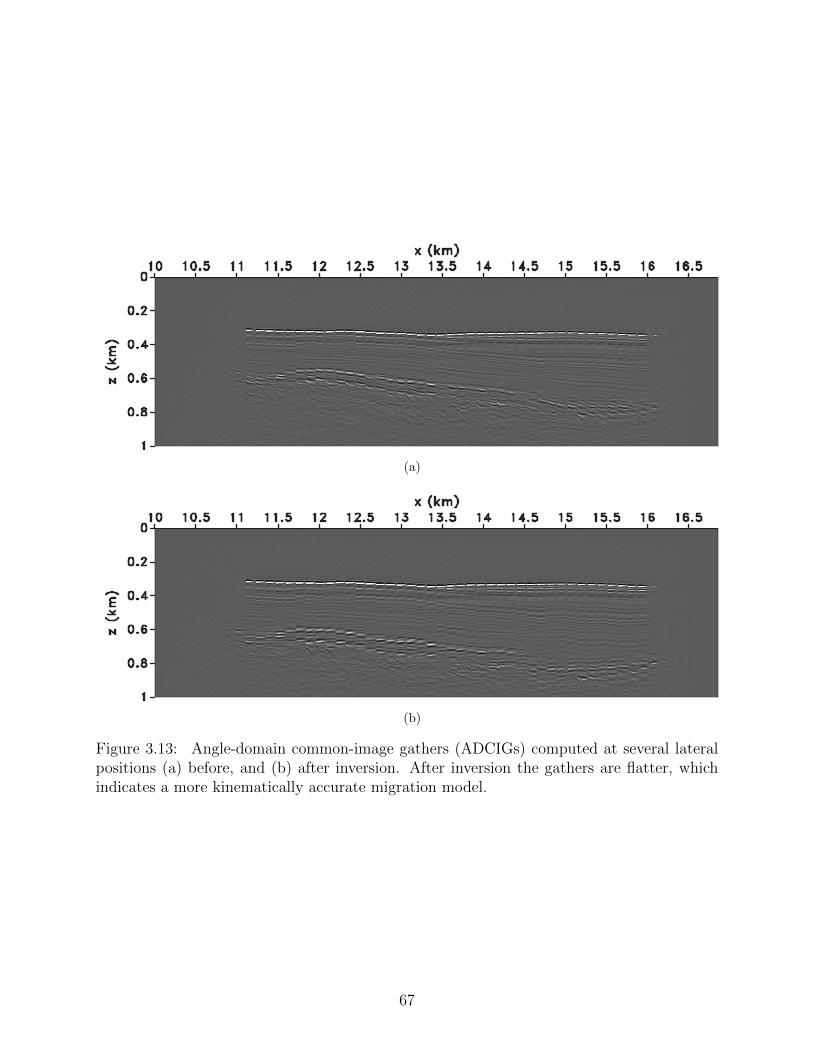
(a)
(b)
Figure 3.13: Angle-domain common-image gathers (ADCIGs) computed at several lateralpositions (a) before, and (b) after inversion. After inversion the gathers are flatter, whichindicates a more kinematically accurate migration model.
67

Figure 3.14: The evolution of the objective function shows that the algorithm convergesafter about 80 iterations.
the correctness of the velocity model used for imaging the survey: when the velocity model
is correct, all shots locate reflectors at the same position, i.e., the image is invariant along
the experiment axis. Several shots are needed to evaluate a velocity error at a single point
in space.
We can evaluate the invariance along the experiment axis by computing the energy of
the first derivative in that dimension. The first derivative acts as a penalty operator by
highlighting and enhancing deviations from the horizontal direction along the shot axis.
The stack of the energy of the first derivative is the differential semblance operator applied
directly in the shot domain (Plessix, 2006; Symes, 1991).
Here, we explore an alternative statement of the semblance principle: when the velocity
model is correct, images from different shots constructively interfere and build up the im-
age perpendicular to the structural dip or parallel to the reflector slope, at every point in
the image space. The structural dip is a commonly extracted attribute and can be linked
to the image itself by means of the gradient-squared tensors (van Vliet and Verbeek, 1995).
Unfortunately, the relationship between wavefields and the dip field is nonlinear: the dip vec-
tor represents the eigenvector associated with the largest eigenvalue of the gradient-squared
tensor. Including the dip variation with respect to model perturbation in the inversion proce-
68

dure is not straightforward, and further research is needed to develop an efficient method to
exploit this information for velocity analysis purposes. Nonetheless, we are able to measure
the semblance of two images through appropriately penalized local correlations of pairs of
images. If the velocity model is correct, the maximum of the local correlation is along the
reflector at every point in the image; if the model is incorrect, the maximum deviates from
the reflector slope. The penalty operator is space-dependent and annihilates the correlation
panels orthogonal to the reflector dip. Because of the dependency on the velocity model,
we measure the dip field at each tomographic iteration; the estimation can be carried out
efficiently using gradient-squared tensors (van Vliet and Verbeek, 1995).
The correlation objective function is superior to the image difference in many respects.
First, the difference between two images depends on image amplitudes that change as a
function of the shot position and cannot be matched point-wise as in the standard imple-
mentation of full-waveform inversion in the data space. The amplitude patterns affect the
residual in the image space and effectively contribute to the adjoint source calculation, even
if the velocity model is correct and the gradient of the objective function is zero (Mulder
and Kroode, 2002). By penalizing local correlations, we reduce the dependence of the ob-
jective function on amplitudes, thus increasing the robustness and reducing the systematic
bias caused by the amplitude differences between the images. A downside of the correlation
operator is the loss of spatial resolution. Correlation in the spatial domain is equivalent
to multiplication in the dual frequency/wavenumber domain; for signals with both finite
spatial support and bandwidth, the multiplication of the spectra decreases the bandwidth,
i.e., increases the width of the signal in the spatial domain. To increase the resolution and
accuracy of the evaluation of the relative shifts between images, deconvolution is a viable
improvement over correlation. If we assume that two images from nearby experiments are
linked by a simple spatial shift, a local deconvolution approach would ideally produce a
bandlimited spatial delta function indicating the direction of apparent displacement. On the
other hand, since deconvolution amplifies the noise in the data (because of the division in
69

the frequency domain), additional care is necessary to stabilize the result.
A thorough study of the effect of the shot distance on the computed gradient would
be beneficial in relation to phenomena such as cycle skipping, which hinders many velocity
analysis strategies (especially but not exclusively in the data domain). The image domain is
intrinsically less prone to cycle skipping problems; nevertheless the question remains about
what happens when two images illuminate rather different areas of the subsurface and the
local correlations cannot be used to estimate a reliable and meaningful shift between the two
images. From our current knowledge and understanding, the shots must be close enough to
provide comparable images of the subsurface and avoid cycle skipping in the image domain.
The sampling of the shot position and the illumination pattern in the subsurface can also
create a scenario in which the two images do not overlap in certain local windows.
Our method is based on locally coherent events, such as locally smooth reflectors. Con-
flicting dips, fault planes, and areas where the definition of a reflection plane is ambiguous
represent open problems because in these areas we cannot define penalty operators. In this
respect, plane-wave migration may represent a valid solution because of the implicit spatial
filtering of the image: each plane-wave reconstructs a particular subset of the dips in the
model, thus reducing the ambiguity in defining the penalty operators. Alternatively, for
complex areas with conflicting dips and complicated geologic features (where there is no
clear definition of the dip field), a more sophisticated design of the penalty operator may be
key to obtaining meaningful residuals and a reliable gradient. The eigenvalues and eigen-
vectors of the gradient-squared tensors (van Vliet and Verbeek, 1995) can be used to define
ellipses that, in turn, may offer a structure-oriented criterion for the definition of the penalty
operators.
In contrast with other techniques in the image space (Biondi and Symes, 2004; Bishop
et al., 1985; Lambare et al., 2004; Xie and Yang, 2008; Yang and Sava, 2010, 2011b), our
approach does not need to explicitly construct and analyse image gathers (or extended
images). A further cost-saving factor is given by the selection of points on the imaged
70

reflectors (Yang and Sava, 2010) and away from complex areas (pinch-outs or areas with
conflicting dips). The computation of the local correlation is carried out at every image
point using the efficient method developed by Hale (2006).
The ability to extract velocity information from pairs of experiments adds a new degree
of freedom for implementing a model update procedure. Here, we indicate two possible
strategies. We can simultaneously include all the shots in the survey in the definition of
the objective function or we can proceed iteratively and update the velocity model using
the information obtained from a single pair of experiments before moving to the next pair.
Nearby shots probe similar portions of the model and provide comparable images; we can
use the information extracted from an initial group to update the model used for imaging
a second group of experiments. Since in any migration velocity analysis scheme we have to
image the entire survey at least once, the iterative update of the model over shots becomes
cost-effective if we actually reduce the number of global migrations of the entire dataset.
In 2D, we can easily define an order for the experiments; in the general 3D scenario, we
have an extra degree of freedom. The definition of the objective function remains the same
but a given shot can have more than 2 neighboring experiments (the acquisition is defined on
a two-dimensional grid). We can generalize the concept of correlation using the semblance
functional (Taner and Koehler, 1969), which is nonlinear in the input signals and makes
the computation of the gradient more involved. We can also separately analyze each pair
of experiments given a reference model. Further research and numerical tests are needed to
assess efficiency and robustness of one strategy over the other.
3.6 Conclusions
We develop an objective function for migration velocity analysis in the shot-image do-
main. Our methodology is based on local image correlations and a reformulation of the
semblance principle involving only small groups of migrated images. The optimization cri-
terion is the minimization of the apparent shift between the migrated images and naturally
leads to a differential semblance optimization problem, which is iteratively solved using a
71

gradient-based method. The linearity of the operators in the objective function makes the
computation of the gradient practical using the adjoint-state method. Our approach is full-
wave because we do not rely on the linearization of the wave extrapolation procedure with
respect to the model parameters to construct a migration velocity analysis operator. We
iteratively solve a nonlinear problem with a gradient-based algorithm and the simulation of
the wavefields is fully nonlinear with respect to the model parameters.
The structural features in the migrated image and the variation of these features as
function of experiment supply valuable information about the model parameters. Here, we
show that it is possible, without constructing common-image gathers , to extract information
about the model from a very limited number of experiments using a warping relationship
between migrated images. We use a few synthetic tests to describe the algorithm and the
behavior of the inversion procedure; we inverted a real 2D marine dataset to demonstrate
the effectiveness of our method.
3.7 Acknowledgments
We would like to thank eni E&P for permission to publish this work and Nicola Bienati
for the valuable conversations on tomography and inversion. The reproducible numerical
examples in this paper use the Madagascar open-source software package freely available
from http://www.reproducibility.org. This research was supported in part by the Golden
Energy Computing Organization at the Colorado School of Mines using resources acquired
with financial assistance from the National Science Foundation and the National Renewable
Energy Laboratory. FP would also like to thank Thomas Cullison for developing the auto-
matic picking algorithm used in this research, Jeff Godwin for developing the interfaces for
the cluster, and Prof. Luis Tenorio for his help and mathematical support.
72
CHAPTER 4
SHOT-DOMAIN 4D TIME-LAPSE SEISMIC VELOCITY ANALYSIS USING
APPARENT IMAGE DISPLACEMENTS
A paper to be submitted to Geophysics
F. Perrone1 and P. Sava1
4.1 Summary
Hydrocarbon production modifies the stress conditions in the subsurface and changes
the model parameters previously estimated from the prospect. The capability to remotely
monitor the changes in the reservoir using seismic data has strategic importance since it
allows us to infer fluid movement and evolution of stress conditions, which are key factors
to enhance recovery and reduce uncertainty and risk during production. A model of the
subsurface parameters is necessary to reconstruct the seismic waves traveling through the
medium and thus correctly image reflectors in the subsurface. Geomechanical changes in the
subsurface can be measured by changes of seismic images obtained from the recorded data of
multiple time-lapse surveys. In this work, we estimate changes of subsurface model param-
eters using the apparent shifts between migrated images obtained by 4D time-lapse seismic
surveys. We assume that the shift between the time-lapse images of the same reflectors is
completely due to the perturbation of the model parameters, and we use the image from
the first (baseline) survey as a reference to estimate this perturbation. The apparent shifts
are measured using penalized local correlations in the image domain, which take advantage
of the local coherency of the reflectors in the image domain and do not explicitly rely on
semblance in common-image gathers. The energy of the estimated displacements defines the
objective function of our optimization scheme. We implement a wavefield tomography algo-
rithm using the adjoint-state method for computing the gradient of the objective function.
1Center for Wave Phenomena, Colorado School of Mines
73
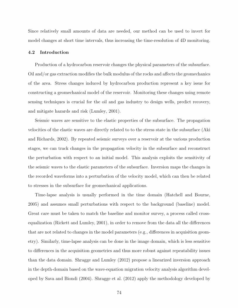
Since relatively small amounts of data are needed, our method can be used to invert for
model changes at short time intervals, thus increasing the time-resolution of 4D monitoring.
4.2 Introduction
Production of a hydrocarbon reservoir changes the physical parameters of the subsurface.
Oil and/or gas extraction modifies the bulk modulus of the rocks and affects the geomechanics
of the area. Stress changes induced by hydrocarbon production represent a key issue for
constructing a geomechanical model of the reservoir. Monitoring these changes using remote
sensing techniques is crucial for the oil and gas industry to design wells, predict recovery,
and mitigate hazards and risk (Lumley, 2001).
Seismic waves are sensitive to the elastic properties of the subsurface. The propagation
velocities of the elastic waves are directly related to to the stress state in the subsurface (Aki
and Richards, 2002). By repeated seismic surveys over a reservoir at the various production
stages, we can track changes in the propagation velocity in the subsurface and reconstruct
the perturbation with respect to an initial model. This analysis exploits the sensitivity of
the seismic waves to the elastic parameters of the subsurface. Inversion maps the changes in
the recorded waveforms into a perturbation of the velocity model, which can then be related
to stresses in the subsurface for geomechanical applications.
Time-lapse analysis is usually performed in the time domain (Hatchell and Bourne,
2005) and assumes small perturbations with respect to the background (baseline) model.
Great care must be taken to match the baseline and monitor survey, a process called cross-
equalization (Rickett and Lumley, 2001), in order to remove from the data all the differences
that are not related to changes in the model parameters (e.g., differences in acquisition geom-
etry). Similarly, time-lapse analysis can be done in the image domain, which is less sensitive
to differences in the acquisition geometries and thus more robust against repeatability issues
than the data domain. Shragge and Lumley (2012) propose a linearized inversion approach
in the depth-domain based on the wave-equation migration velocity analysis algorithm devel-
oped by Sava and Biondi (2004). Shragge et al. (2012) apply the methodology developed by
74

Yang and Sava (2011a) to 4D seismic monitoring and uses the adjoint-state method (Fichtner
et al., 2006), which removes the linearity assumptions. By operating directly in the depth
domain without linearity assumptions, this inversion can handle strong errors in the velocity
model.
Wave-equation migration velocity analysis (MVA) (Sava and Biondi, 2004) and image-
domain waveform tomography (Yang and Sava, 2011a) require complete aperture to correctly
construct the image perturbation that drives the tomographic procedure and to evaluate
focusing in the subsurface, respectively. The requirements for the acquisition geometry can be
relaxed using the approach proposed by Yang and Sava (2012); nonetheless, a large aperture
is necessary for resolution purposes. We advocate the use of local image correlations (Hale,
2006) and dip-dependent penalty operators to measure the relative displacement between
shot-migrated images and then use the inversion technique of Perrone and Sava (2012c) to
evaluate a model update following production. Penalized ocal image correlations allow us
to estimate the velocity model errors shot by shot. The image-domain approach is robust
against repeatability issues, such as errors in the shot and receiver positions, and the adjoint-
state method allows us to implement a nonlinear inversion procedure, which is effective for
large and complex model updates.
4.3 Theory
Perrone and Sava (2012c) restate the semblance principle considering locally coherent
events in the image domain: the velocity model is correct when the images from different
neighboring experiments show conformal features, that is, when the dips of the reflectors in
the two images are point-wise consistent. This criterium can be applied to migration velocity
analysis using local image correlations to evaluate the relative movement of the two images
with respect to their structural dips. We can use the same idea for 4D time-lapse seismic and
compare the images obtained from the baseline and monitor survey. In this case, we measure
shifts of the monitor image with respect to the baseline, which represents the reference. The
shift is measured along the normal to the reflector (in the dip direction).
75

We set an optimization problem by defining the objective function (Perrone and Sava,
2012c)
J (m) =1
2‖∑λ
P (x,λ) c (x,λ) ‖2x, (4.1)
where c (x,λ) =∫w (x− ξ)Rbsl
(ξ − λ
2
)Rmon
(ξ + λ
2
)dξ is the local correlation of the base-
line image Rbsl (x) and the monitor image Rmon (x), and P (x,λ) is a penalty operator that
highlights features which are related to velocity errors. The correlations are computed in
local seamlessly overlapping windows w (x), and the variable m (x) denotes the model (slow-
ness squared, slowness, velocity, etc.). When the velocity model is correct, the two images are
perfectly aligned and the residual∑λ
P (x,λ) c (x,λ), a proxy for the relative displacement,
is at minimum.
While we assume that the shifts between the migrated baseline and monitor survey are
related to the errors in the velocity model, this is not necessarily true since changes in the
stress conditions can cause compaction of the reservoir and lead to subsidence, that is physical
movement of all the reflectors above the reservoir. Although subsidence up to 12 m due to
hydrocarbon production has been observed and reported in the literature (for example, in
the Ekofisk field in the North Sea), shifts in the subsurface are usually negligible compared
to the wavelength of the seismic signal (typically these movements can be in the order of a
meter between the top and bottom of the reservoir (Hatchell and Bourne, 2005)); it is thus
safe to assume that the estimated shifts in the reflector positions are due to changes in the
migration model and not to changes of the positions of the interfaces. This is especially true
when monitor surveys are performed at relatively short time intervals.
We compute the gradient of the objective function in equation 4.1 using the adjoint-state
method (Fichtner et al., 2006). The migrated images are defined as the zero-lag time-
correlation of the source and receiver wavefield us (x, t) and ur (x, t), which are extrapolated
in a model m (x) of the subsurface. The wavefields are computed by solving the wave-
equations
76
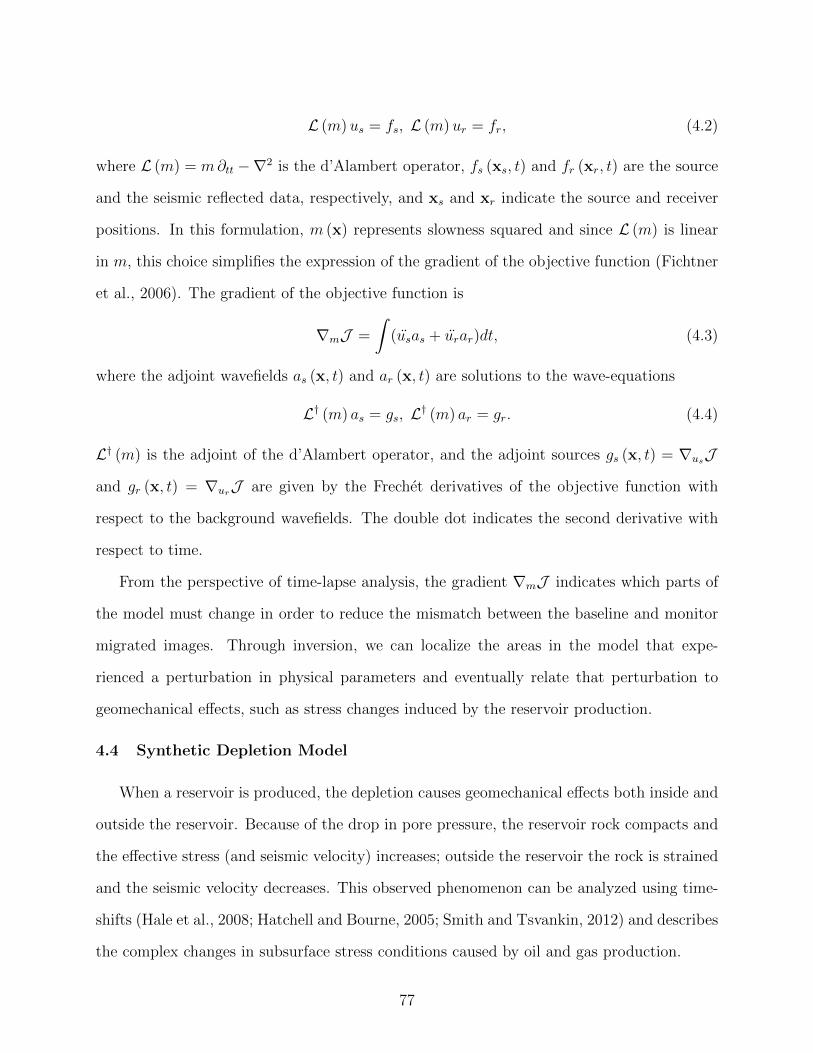
L (m)us = fs, L (m)ur = fr, (4.2)
where L (m) = m∂tt −∇2 is the d’Alambert operator, fs (xs, t) and fr (xr, t) are the source
and the seismic reflected data, respectively, and xs and xr indicate the source and receiver
positions. In this formulation, m (x) represents slowness squared and since L (m) is linear
in m, this choice simplifies the expression of the gradient of the objective function (Fichtner
et al., 2006). The gradient of the objective function is
∇mJ =
∫(usas + urar)dt, (4.3)
where the adjoint wavefields as (x, t) and ar (x, t) are solutions to the wave-equations
L† (m) as = gs, L† (m) ar = gr. (4.4)
L† (m) is the adjoint of the d’Alambert operator, and the adjoint sources gs (x, t) = ∇usJ
and gr (x, t) = ∇urJ are given by the Frechet derivatives of the objective function with
respect to the background wavefields. The double dot indicates the second derivative with
respect to time.
From the perspective of time-lapse analysis, the gradient ∇mJ indicates which parts of
the model must change in order to reduce the mismatch between the baseline and monitor
migrated images. Through inversion, we can localize the areas in the model that expe-
rienced a perturbation in physical parameters and eventually relate that perturbation to
geomechanical effects, such as stress changes induced by the reservoir production.
4.4 Synthetic Depletion Model
When a reservoir is produced, the depletion causes geomechanical effects both inside and
outside the reservoir. Because of the drop in pore pressure, the reservoir rock compacts and
the effective stress (and seismic velocity) increases; outside the reservoir the rock is strained
and the seismic velocity decreases. This observed phenomenon can be analyzed using time-
shifts (Hale et al., 2008; Hatchell and Bourne, 2005; Smith and Tsvankin, 2012) and describes
the complex changes in subsurface stress conditions caused by oil and gas production.
77

In order to test our velocity estimation procedure, we use a geomechanical model used
by Fuck et al. (2009) and Smith and Tsvankin (2012) to obtain the model parameters for
a reservoir under depletion. The geomechanical model simulates the response of a single-
compartment rectangular reservoir comprised of and embedded in homogeneous Berea sand-
stone (Figure 4.1). The depth of the reservoir is z = 1.5 km, the thickness is 0.1 km, and the
width is 2.0 km. The parameters of wave propagation obtained from laboratory measure-
ments are Vp = 2300 m/s, Vp = 1456, and ρ = 2140 kg/m3. The details of the geomechanical
simulation can be found in Smith and Tsvankin (2012).
We generate data with acoustic finite-differences using density reflectors at various depths
and with absorbing boundary conditions on each side of the model (Figure 4.2(a)).
The initial velocity model is homogenous and equal to 2.07 km/s velocity. The value
is obtained by reducing the laboratory values for Berea sandstone by 10% to account for
the difference between static and dynamic stiffnesses. Figure 4.2(b) shows a model of the
reservoir undergoing a 20% depletion, that is the change in pore pressure is equal to 20%
of the confining pressure Smith and Tsvankin (2012). Observe the complex pattern of the
velocity anomaly outside the reservoir. The velocity model perturbation inside the reservoir
is about +15% with respect to the baseline model. The sensitivity of our velocity error
measure as a function of depletion of the reservoir is shown in Figure 4.3. As depletion
increases the monitor image becomes more and more distorted and strong headwaves are
generated, which represent an additional source of noise. As a consequence, the objective
function loses sensitivity at elevated depletion percentages.
We place a single shot at x = 1.5 km at the surface and perform 3 inversion tests.
The first experiment represents an “ideal” scenario in which we have a full (at the surface)
repeatable survey. We invert the velocity anomaly and use it to study the sensitivity of
our algorithm when the acquisition is limited, as a marine-streamer case, and when the
acquisition is both limited and not perfectly repeatable, e.g., because of errors in source and
receivers positioning.
78

ReservoirPfluidPeff = Pcon-αPfluid
Pcon
2.0 km
0.1 km
1.5 km
ΔPfluid = - ξPcon
x
z
Figure 4.1: Reservoir geometry after Smith and Tsvankin (2012). Pore-pressure (PP =Pfluid) reduction occurs only within the reservoir, resulting in an anisotropic velocity field dueto the excess stress and strain. The reservoir is comprised of and embedded in homogeneousBerea sandstone (VP = 2300 ms−1, VS = 1456 ms−1, ρ = 2140 kgm−3). The Biot coefficient(α) for the reservoir is 0.85. Velocities in the model are reduced by 10% from the laboratoryvalues to account for the difference between static and dynamic stiffnesses in low-porosityrocks. The change in pore pressure ∆Pfluid is expressed as a percentage ξ of the confiningpressure Pcon.
79
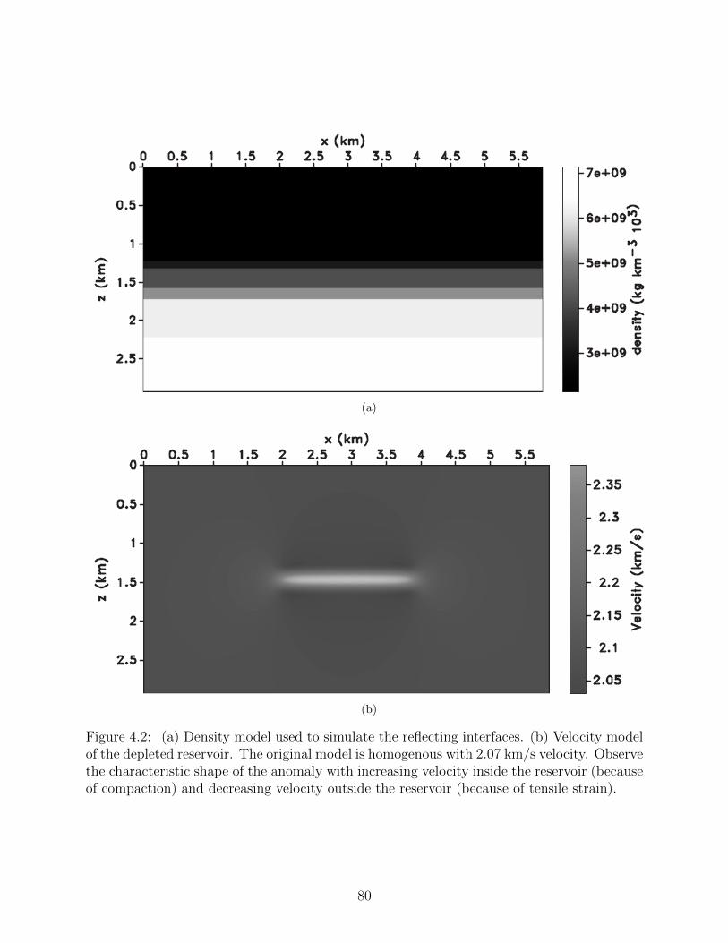
(a)
(b)
Figure 4.2: (a) Density model used to simulate the reflecting interfaces. (b) Velocity modelof the depleted reservoir. The original model is homogenous with 2.07 km/s velocity. Observethe characteristic shape of the anomaly with increasing velocity inside the reservoir (becauseof compaction) and decreasing velocity outside the reservoir (because of tensile strain).
80
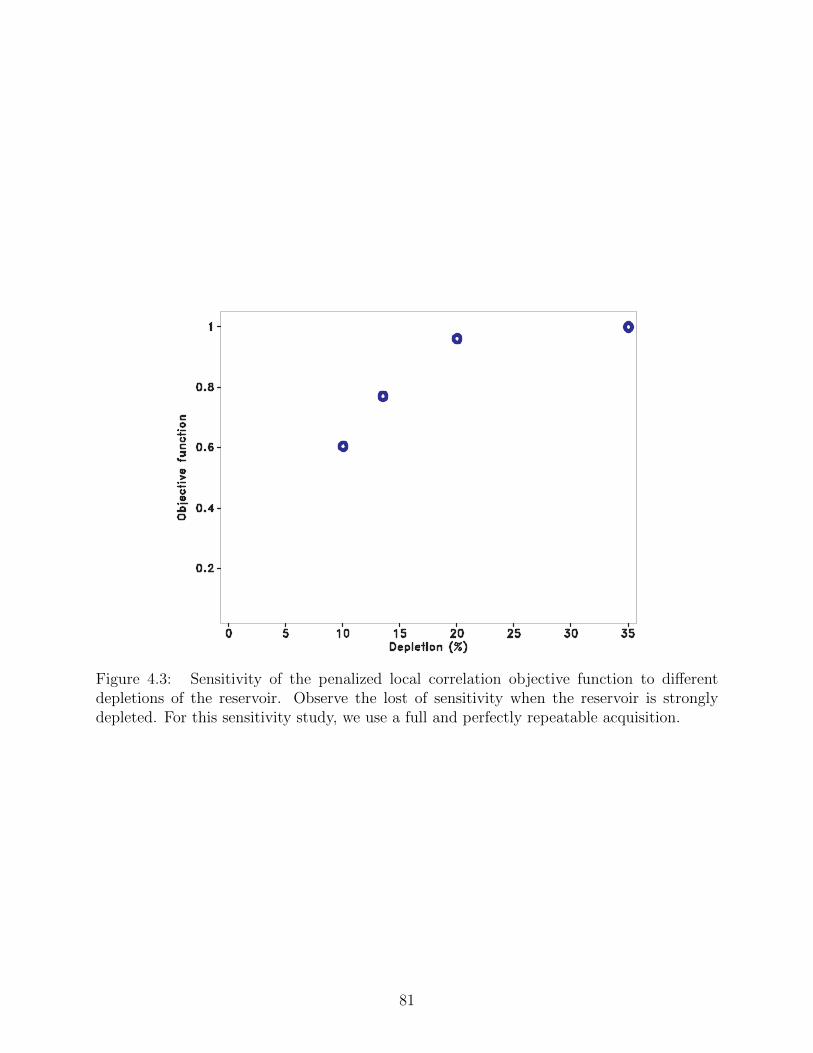
Figure 4.3: Sensitivity of the penalized local correlation objective function to differentdepletions of the reservoir. Observe the lost of sensitivity when the reservoir is stronglydepleted. For this sensitivity study, we use a full and perfectly repeatable acquisition.
81
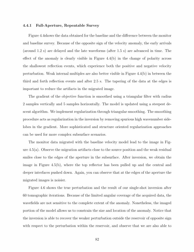
4.4.1 Full-Aperture, Repeatable Survey
Figure 4.4shows the data obtained for the baseline and the difference between the monitor
and baseline survey. Because of the opposite sign of the velocity anomaly, the early arrivals
(around 1.2 s) are delayed and the late waveforms (after 1.5 s) are advanced in time. The
effect of the anomaly is clearly visible in Figure 4.4(b) in the change of polarity across
the shallowest reflection events, which experience both the positive and negative velocity
perturbation. Weak internal multiples are also better visible in Figure 4.4(b) in between the
third and forth reflection events and after 2.5 s. The tapering of the data at the edges is
important to reduce the artifacts in the migrated image.
The gradient of the objective function is smoothed using a triangular filter with radius
2 samples vertically and 5 samples horizontally. The model is updated using a steepest de-
scent algorithm. We implement regularization through triangular smoothing. The smoothing
procedure acts as regularization in the inversion by removing spurious high wavenumber side-
lobes in the gradient. More sophisticated and structure oriented regularization approaches
can be used for more complex subsurface scenarios.
The monitor data migrated with the baseline velocity model lead to the image in Fig-
ure 4.5(a). Observe the migration artifacts close to the source position and the weak residual
smiles close to the edges of the aperture in the subsurface. After inversion, we obtain the
image in Figure 4.5(b), where the top reflector has been pulled up and the central and
deeper interfaces pushed down. Again, you can observe that at the edges of the aperture the
migrated images is noisier.
Figure 4.6 shows the true perturbation and the result of our single-shot inversion after
60 tomographic iterations. Because of the limited angular coverage of the acquired data, the
wavefields are not sensitive to the complete extent of the anomaly. Nonetheless, the imaged
portion of the model allows us to constrain the size and location of the anomaly. Notice that
the inversion is able to recover the weaker perturbation outside the reservoir of opposite sign
with respect to the perturbation within the reservoir, and observe that we are also able to
82
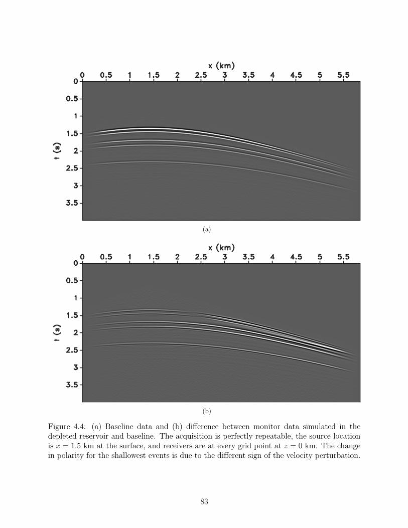
(a)
(b)
Figure 4.4: (a) Baseline data and (b) difference between monitor data simulated in thedepleted reservoir and baseline. The acquisition is perfectly repeatable, the source locationis x = 1.5 km at the surface, and receivers are at every grid point at z = 0 km. The changein polarity for the shallowest events is due to the different sign of the velocity perturbation.
83

(a)
(b)
Figure 4.5: (a) Migrated monitor image obtained using the baseline model and (b) migratedmonitor image after inversion with full receiver coverage at the surface. The central anddeeper reflectors are moved downward, which the shallowest interface is pulled up. The mi-gration artifacts are due to truncation of the acquisition and critical reflections (headwaves)from the anomaly in the depleted reservoir.
84

(a)
(b)
Figure 4.6: (a) Actual time-lapse model perturbation and (b) inverted perturbation after60 iterations of wavefield tomography with full receiver coverage at the surface. Notice thatwe are able to correctly image the anomaly and also constrain its lateral extent at aboutx = 2 km.
85

correctly image the left side of the anomaly thus correctly constraining its lateral extent.
Figure 4.7 shows the shifts between the baseline and monitor migrated images before and
after inversion. Black indicated a downward shift whereas white indicate an upward shift.
Before inversion the shallower and deeper reflectors are shifted in opposite direction because
of the different sign of the anomaly inside and outside the reservoir (see Figure 4.6(a)). After
inversion the reflectors are better aligned; inversion warps the monitor image into the baseline
image and returns the velocity anomaly that corrects the shifts of the imaged interfaces. We
can observe some spurious strong residual shifts at the edges of the illumination in the
migrated domain, which are due to residual migration artifacts that contaminate the image.
The migration artifacts are the principal source of noise in this example: observe the shifts
that are measured close to the source position (x = 1.0 km), which are completely spurious
because they are measured along migration smiles due to truncation at the edges of the
acquisition. The fewer data close to the edges of the acquisition do not allow us to produce
a clean image and thus to constrain the geometry of the reflectors. As a consequence, the
gradient of the objective function and the model update are less reliable than in the central
part of aperture (from x = 1.0 km to x = 2.0 km).
4.4.2 Limited-Aperture, Repeatable Survey
In order to model a more realistic marine acquisition, we simulate a single-side, marine
streamer acquisition. Our experiment uses a single shot-gather with the source located at
x = 1.5 km and with a streamer 3.2 km long. The length of the cable is about the same as
the lateral extent of the reservoir. The streamer carries 200 evenly spaced receivers and the
receiver spacing is 8 m. The acquisition is perfectly repeatable, i.e., the position of source
and receiver is identical in the baseline and monitor survey.
Figure 4.8 shows the simulated data with limited aperture and the difference between the
monitor and baseline dataset. By reducing the angular coverage, we reduce the lateral extent
of the imaged reflectors, which affects the computed gradient of the objective function.
86
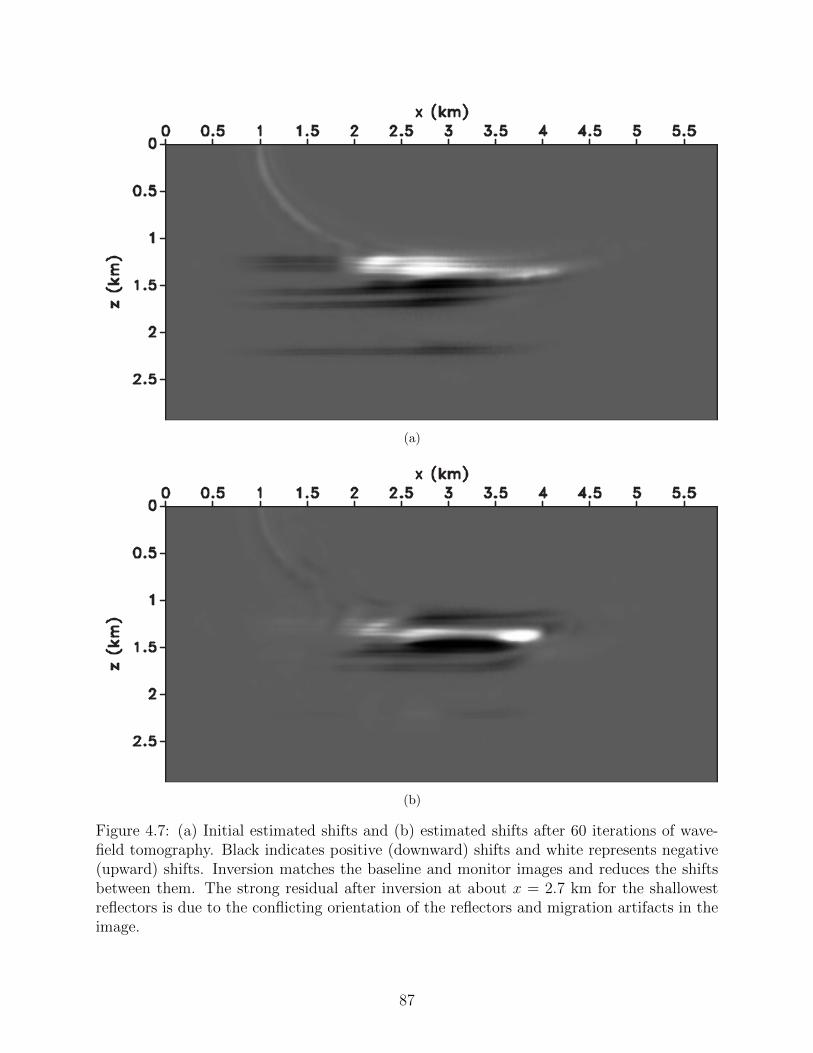
(a)
(b)
Figure 4.7: (a) Initial estimated shifts and (b) estimated shifts after 60 iterations of wave-field tomography. Black indicates positive (downward) shifts and white represents negative(upward) shifts. Inversion matches the baseline and monitor images and reduces the shiftsbetween them. The strong residual after inversion at about x = 2.7 km for the shallowestreflectors is due to the conflicting orientation of the reflectors and migration artifacts in theimage.
87
(a)
(b)
Figure 4.8: (a) Baseline data and (b) difference between monitor data simulated in thedepleted reservoir and baseline. We reduced the receiver coverage to simulate a marine-streamer acquisition. Observe the polarity change of the shallowest reflection events in thedifferential dataset due to the sign change of the velocity anomaly.
88

(a)
(b)
Figure 4.9: (a) migrated monitor image obtained using the baseline model and (b) migratedmonitor image after inversion with reduced receiver coverage. The central and deeper reflec-tors are moved downward, which the shallowest interface is pulled up. Observe the migrationartifacts which represent the main source of noise for inversion. The limited acquisition mutesthe close-to-critical reflections from the reservoir and reduces the migration artifacts in themigrated image.
89
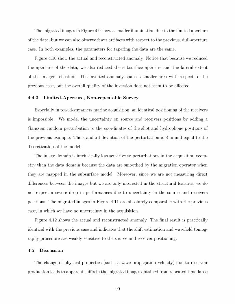
The migrated images in Figure 4.9 show a smaller illumination due to the limited aperture
of the data, but we can also observe fewer artifacts with respect to the previous, dull-aperture
case. In both examples, the parameters for tapering the data are the same.
Figure 4.10 show the actual and reconstructed anomaly. Notice that because we reduced
the aperture of the data, we also reduced the subsurface aperture and the lateral extent
of the imaged reflectors. The inverted anomaly spans a smaller area with respect to the
previous case, but the overall quality of the inversion does not seem to be affected.
4.4.3 Limited-Aperture, Non-repeatable Survey
Especially in towed-streamers marine acquisition, an identical positioning of the receivers
is impossible. We model the uncertainty on source and receivers positions by adding a
Gaussian random perturbation to the coordinates of the shot and hydrophone positions of
the previous example. The standard deviation of the perturbation is 8 m and equal to the
discretization of the model.
The image domain is intrinsically less sensitive to perturbations in the acquisition geom-
etry than the data domain because the data are smoothed by the migration operator when
they are mapped in the subsurface model. Moreover, since we are not measuring direct
differences between the images but we are only interested in the structural features, we do
not expect a severe drop in performances due to uncertainty in the source and receivers
positions. The migrated images in Figure 4.11 are absolutely comparable with the previous
case, in which we have no uncertainty in the acquisition.
Figure 4.12 shows the actual and reconstructed anomaly. The final result is practically
identical with the previous case and indicates that the shift estimation and wavefield tomog-
raphy procedure are weakly sensitive to the source and receiver positioning.
4.5 Discussion
The change of physical properties (such as wave propagation velocity) due to reservoir
production leads to apparent shifts in the migrated images obtained from repeated time-lapse
90

(a)
(b)
Figure 4.10: (a) Actual time-lapse model perturbation and (b) inverted perturbation after 60iterations of wavefield tomography. Notice that we are able to correctly image the anomalyand also constrain its lateral extent at about x = 2 km. The reduced receiver coveragereduces the extent of the reconstructed anomaly compared to Figure 4.6(b).
91
(a)
(b)
Figure 4.11: (a) migrated monitor image obtained using the baseline model and (b) migratedmonitor image after inversion in the case of a non-repeatable survey. The monitor data areacquired using source and receivers at different positions with respect to the baseline survey,but the imaged reflectors are weakly sensitive to small perturbations of the acquisition.
92

(a)
(b)
Figure 4.12: (a) Actual time-lapse model perturbation and (b) inverted perturbation after 60iterations of wavefield tomography. Notice that we are able to correctly image the anomalyand also constrain its lateral extent at about x = 2 km. Despite the error in the sourceand receiver location, the inversion result is indistinguishable from the repeatable case inFigure 4.10(b).
93

seismic surveys of the field. Because the velocity model used in migration is calibrated on
the baseline survey, the reflectors in the monitor survey are slightly mispositioned because
we are not accounting for the perturbation of the model due to the production of the field.
By matching the baseline and monitor migrated images for single shots, we can translate the
apparent image shift into a model perturbation. This approach is fully shot-based since the
basic building blocks of the inversion procedure are the single-shot migrated images. This
feature is advantageous in a real production scenario when it is difficult to repeat a complete
survey because of physical obstructions in the field (such as platforms) which can cause big
illumination holes in the images. Conducting a complete survey over a producing field is also
costly because production must be stopped during acquisition in order to reduce the noise in
the seismic data. Our technique addresses this practical problem and can potentially allow
for fast and frequent surveys over a producing reservoir.
The advantage of our technique over methods based on wavefield focusing (Girard and
Vasconcelos, 2010; Shragge et al., 2012) comes from the reduced implementation cost (no ex-
tended images are needed) and the robustness against poor illumination. By analyzing single-
shot migrated images, we are automatically taking into account the illumination pattern of
the experiments; on the contrary, focusing measures require full aperture or point-spread
function compensation to equalize the complex illumination patterns due to the geologic
structures and/or acquisition geometry. In this work, we recover a portion of the anomaly
from a single migrated shot, which would be impossible using any technique based on focus-
ing. However, a single shot illuminates the medium using a limited set of directions and, in
simple settings like the one in our synthetic experiments, every point on the imaged reflectors
is illuminated by a single ray. The local coherence of the reflectors allows us to constrain
the inversion, nonetheless, more shots are necessary to better reconstruct the spectrum of
the anomaly.
In general, velocity anomalies due to reservoir stimulation or production are small relative
to the velocity error in the initial stages of model building. Moreover, the baseline velocity
94
model should already be calibrated and thus be expected to produce a high-quality migrated
image. Therefore, our technique based on apparent image shifts is more robust for time-lapse
seismic monitoring than for the original migration velocity analysis, when we match a set of
inaccurate images.
The main source of noise for the algorthm is related to migration artifacts that may
contaminate the single shot migrated images. These artifacts can be due to truncation in
the acquisition or to the actual complexity of the velocity medium. In the first case, careful
tapering of the data can help reducing or eliminating the migration smiles; in the latter case,
nothing can be actually done in the migrated-shot domain. The migration operator is the
adjoint (not the inverse) of the forward Born operator, Stolk and Symes (2004) study and
explain the nature of these artifacts that appear in strongly refractive media and are related
to the inability of the migration operator to handle multipathing using only surface-related
coordinates.
4.6 Conclusions
Local correlations evaluated in the image domain allow us to assess the quality of the
velocity model from a limited number of migrated images. In 4D seismic applications,
we can quickly estimate a perturbation of the migration model by comparing shot images
from baseline and monitor surveys. In the image domain, we measure the consistency and
similarity of locally coherent events, like the local dip of the reflectors; these features are
weakly sensitive to differences in the acquisition geometry and make our approach more
robust against survey repeatability issues as compared to alternative strategies in the data
domain. The method is able to recover the relative error in the model and does not require
separate velocity analysis for baseline and monitor surveys in order to estimate the differences
between the models inverted independently.
95

4.7 Acknowledgment
We would like to thank Jyoti Behura for interesting discussions about 4D time-lapse
seismic and for encouraging FP to look into this problem. This work was supported by
the sponsors of the Consortium Project on Seismic Inverse Methods for Complex Structures.
The reproducible numerical examples in this paper use the Madagascar open-source software
package freely available from http://www.ahay.org and the Mines JTK freely available at
https://github.com/dhale/jtk.
96
CHAPTER 5
IMAGE-WARPING WAVEFORM TOMOGRAPHY
A paper to be submitted to Geophysical Prospecting
F. Perrone1 and P. Sava1
5.1 Summary
Imaging the change in physical parameters in the subsurface requires an estimate of the
long wavelength component of the same parameters in order to reconstruct the kinematics
of the waves propagating in the subsurface. The model is unknown and must be estimated
from the same data. One can try to reconstruct the method by matching the recorded data
with modeled waveforms extrapolated in a trial model of the medium. Alternatively, assum-
ing a trial model, one can obtain a set of images of the reflectors from a number of seismic
experiments and match the locations of the imaged interfaces. Apparent displacements be-
tween migrated images contain information about the velocity model and can be used for
velocity analysis. A number of methods are available to estimate the displacement between
images; in this paper, we compare shot-domain differential semblance (image difference),
penalized local correlations, and image-warping. We show that the image-warping vector
field is a more reliable tool for estimating displacements between migrated images and leads
to a more robust velocity analysis procedure. By using image-warping, we can redefine the
differential semblance optimization problem with a residual that is more robust against cycle-
skipping than the direct image difference. However, the adjoint-state calculations for this
new objective function are excessively complicated and hide the physical intuitions about the
tomographic problem. We propose a second approach that has straightforward implementa-
tion and reduced computational cost compared to the adjoint-state method calculations. We
1Center for Wave Phenomena, Colorado School of Mines
97

also discuss the weakness of migration velocity analysis in the migrated-shot domain in the
case of highly refractive media, when the Born modeling operator is far from being unitary
and thus its adjoint operator (the migration operator) poorly approximates the inverse.
5.2 Introduction
Determining accurate propagation velocities in the subsurface is crucial in seismic imag-
ing and exploration geophysics. A kinematically accurate velocity model allows us to cor-
rectly reconstruct Green’s functions and thus precisely image the subsurface discontinuities
responsible for the data acquired at the surface or in boreholes. An accurate image of the
geologic structure is key for planning drilling operations and for reducing hazards associated
with drilling through faults. Seismic propagation velocities are sensitive to the stress condi-
tions in the subsurface and carry information about the orientation of the principal stresses
and overpressures (Carcione, 2007), which are both important for mitigating hazards during
drilling operations and reducing risk in production.
In recent years, a main distinction has been drawn between methods that recover the
velocity model by matching the recorded data with simulated synthetic wavefields modeled
in a trial velocity model (Pratt, 1999; Sirgue and Pratt, 2004; Tarantola, 1984), and methods
that focus on optimizing properties of the migrated images (Al-Yahya, 1989; Albertin et al.,
2006; Biondi and Sava, 1999; Chavent and Jacewitz, 1995; Faye and Jeannot, 1986; Fowler,
1985; Sava et al., 2005). Full-waveform inversion is the name used to indicate techniques that
operate in the data domain and focus on the minimization of some functional of the data
residual. Migration velocity analysis, or image-domain tomography, identifies all methods
that reconstruct the velocity model by analyzing the similarity between migrated images.
Full-waveform inversion is simple to implement, but it is very sensitive to every incon-
sistency between the recorded and modeled data. It requires an accurate parametrization
of the physics of wave propagation, knowledge of the source signature, and a kinematically
reliable starting model in order to converge to the global minimum of the objective function
(Kelly et al., 2010; Santosa and Symes, 1989). Migration velocity analysis is not as sensitive
98

to errors in the source signature and it is more robust against errors in the initial veloc-
ity model; it is characterized by an objective function which is convex over a wide range
of model perturbations and thus intrinsically more suitable for gradient-based optimization
procedures. Nonetheless, as it ignores the amplitude information in the data for inversion
purposes, migration velocity analysis cannot achieve the high-resolution results that full-
waveform inversion promises in the ideal scenario (Warner et al., 2012). Migration velocity
analysis is conventionally used to produce a kinematically accurate model to initialize full-
waveform inversion for refining the velocity with high-resolution details. In this work, we are
interested in the reconstruction of the long wavelength component of the model parameters
and thus we focus on image-domain tomography.
Migration velocity analysis is based on the idea that the subsurface is time-invariant on
the time scale of the seismic experiment. The images obtained by seismic migration from a
series of experiments must agree on the position of the reflectors in the subsurface since the
structures that reflect the energy injected by our sources do not change over time. This is
the idea behind the semblance principle (Al-Yahya, 1989; Sattlegger, 1975).
Differential Semblance Optimization (DSO) is a popular solution for measuring the con-
sistency of a set of images and correcting the errors in the migration velocity model (Symes,
1993). Applications of DSO include both regularization for data domain inversion (Plessix,
2006; Symes and Carazzone, 1991) and stand-alone migration velocity analysis techniques
in an extended space (Shen and Symes, 2008; Symes, 2008).
Shot-domain migrated images are obtained by applying the adjoint single-scattering Born
operator to the acquired data. Because the migration operator is an adjoint and not an
inverse operator, in extremely refractive media, the individual migrated images can be con-
taminated by kinematic artifacts (Stolk and Symes, 2004). This problem is addressed by
stacking, which makes migration an approximation of the inverse operator up to a dip-
dependent scaling factor. For velocity analysis, we want to preserve the dimensionality or
the data and avoid stacking. Data can be mapped in the image domain as a function of
99
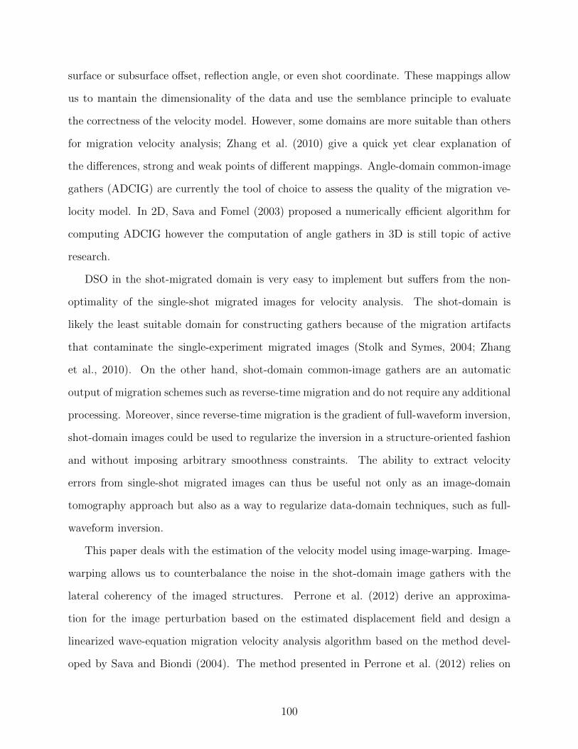
surface or subsurface offset, reflection angle, or even shot coordinate. These mappings allow
us to mantain the dimensionality of the data and use the semblance principle to evaluate
the correctness of the velocity model. However, some domains are more suitable than others
for migration velocity analysis; Zhang et al. (2010) give a quick yet clear explanation of
the differences, strong and weak points of different mappings. Angle-domain common-image
gathers (ADCIG) are currently the tool of choice to assess the quality of the migration ve-
locity model. In 2D, Sava and Fomel (2003) proposed a numerically efficient algorithm for
computing ADCIG however the computation of angle gathers in 3D is still topic of active
research.
DSO in the shot-migrated domain is very easy to implement but suffers from the non-
optimality of the single-shot migrated images for velocity analysis. The shot-domain is
likely the least suitable domain for constructing gathers because of the migration artifacts
that contaminate the single-experiment migrated images (Stolk and Symes, 2004; Zhang
et al., 2010). On the other hand, shot-domain common-image gathers are an automatic
output of migration schemes such as reverse-time migration and do not require any additional
processing. Moreover, since reverse-time migration is the gradient of full-waveform inversion,
shot-domain images could be used to regularize the inversion in a structure-oriented fashion
and without imposing arbitrary smoothness constraints. The ability to extract velocity
errors from single-shot migrated images can thus be useful not only as an image-domain
tomography approach but also as a way to regularize data-domain techniques, such as full-
waveform inversion.
This paper deals with the estimation of the velocity model using image-warping. Image-
warping allows us to counterbalance the noise in the shot-domain image gathers with the
lateral coherency of the imaged structures. Perrone et al. (2012) derive an approxima-
tion for the image perturbation based on the estimated displacement field and design a
linearized wave-equation migration velocity analysis algorithm based on the method devel-
oped by Sava and Biondi (2004). The method presented in Perrone et al. (2012) relies on
100

several approximations and linearizations: the wave-equation migration velocity analysis op-
erator is obtained from the phase-shift continuation operator. The entire inversion procedure
stems from the particular form of the extrapolation operator that allows one to derive a lin-
earized operator which links perturbation in the image space to perturbation in the model
(slowness) parameters. Because of the strong assumption of a phase-shift continuation wave-
extrapolator, this method cannot be applied to images obtained using different engines (for
example, with reverse-time migration). Moreover, events that are not correctly handled by
the extrapolation operator (for example, diving waves and overturning reflections) become
noise for the inversion scheme. In order to generalize the wave-equation migration velocity
analysis method for nonlinear inversion, Perrone and Sava (2012b) propose an image-domain
wavefield tomography approach where the residual is computed from estimates of local shifts
between migrated images. The method presented in Perrone and Sava (2012b) involves the
solution of the full two-way wave equation and thus integrates reverse-time migration into
the inversion procedure. The shifts are obtained from penalized local correlations of images
from nearby experiments, and the adjoint-state method allows us to compute the gradient
of the objective function for implementing a local gradient-based nonlinear inversion. The
method shows weak points when reflectors are located near the acquisition surface and when
several reflectors fall inside the same local window, thus biasing the computation of the local
correlations through the crosstalk between the closely spaced events.
We extend the linearized wave-equation migration velocity analysis algorithm of Perrone
et al. (2012) to incorporate a two-way extrapolation engine and to directly exploit the dis-
placement field. The displacement vector field is used to estimate an image perturbation;
then through single-scattering Born modeling, the wavefield perturbation is computed. The
correlation between the scattered and background wavefields represents the kernel for the
model update. We compare the objective functions based on DSO, local image correlations,
and image-warping, and show that the displacement field leads to a robust objective function
and model update.
101

5.3 Theory
Differential Semblance Optimization in the shot-image domain minimizes the energy of
the difference of neighboring images (Symes, 1993):
JDSO (m) =1
2
∑i
‖Ri+1 −Ri‖2 , (5.1)
where Ri (x) is the migrated image obtained from the ith shot, m (x) represents the model
parameter, and x = (x, y, z) is the position vector. Perrone et al. (2012) show that the
objective function in equation 5.1 can be approximated using the concept of image-warping
as
JWARP (m) =1
2
∑i
‖∇Ri · ui‖2 , (5.2)
where ui (x) is the displacement vector field that maps Ri into Ri+1 and ∇Ri is the gradient
of the migrated image. Image-warping is more robust against cycle skipping and leads to
smoother sensitivity kernels for image-domain tomography. Perrone et al. (2012) also show
that the quantity ∇Ri · ui can be related to the geometrical relations between displacement
and dip of the imaged structures; in particular, when the velocity model is accurate, the dip
and displacement vector field are point-wise orthogonal.
Perrone et al. (2012) use the approximation of the image difference in equation 5.2 in the
framework of the wave-equation migration velocity analysis algorithm developed by Sava
and Biondi (2004). Through a linear operator obtained from the phase-shift migration
operator, the image perturbation ∇Ri · ui is related to an associated slowness perturbation.
By solving a series of linear problems with the image perturbation as input data, one can
then reconstruct the slowness perturbation.
Displacement vectors u are obtained by an iterative search of the maximum of local
correlations and warping of the input images; the algorithm is the same used for measuring
the apparent shift between migrated images in 4D seismic processing (Hale et al., 2008).
The displacement vector field is such that
102

Ri (x + u) = Ri+1 (x) , (5.3)
and is obtained by computing the (possibly) fractional correlation lag that maximizes the
local correlation panels:
u (x) = arg maxλ
c (x,λ) , (5.4)
where c (x,λ) =∫w(x)
Ri
(ξ − λ
2
)Ri+1
(ξ + λ
2
)dξ is the local correlation of two images Ri (x)
and Ri+1 (x), and w (x) are seamlessly overlapping windows. The arg max operator is not
differentiable and thus one cannot compute the Frechet derivative with respect to the model
parameters directly. Because of this, the development of a fully nonlinear inversion scheme
is not straightforward. Perrone and Sava (2012b) use penalized local correlations between
migrated images to measure the shift normal to the structural dip. Their objective function
is the energy of the estimated normal shift. Penalized local correlations can be differentiated
with respect to the state variables and allow one to use the adjoint-state method to compute
the gradient of the objective function (Fichtner et al., 2006; Lions, 1972).
A rigorous adjoint-state calculation for the objective function in equation 5.2 can be
worked out using the idea of connective functions introduced by Luo and Schuster (1991) for
traveltime tomography. The major difference of using connective functions in the framework
of migration velocity analysis is the higher dimensionality of the image space compared to
the data domain. In the data domain, the shifts are one-dimensional (along the time axis,
between observed and synthetic traces); in the image domain, the displacement vectors are
multidimensional, which considerably increases the computation complexity and cost of the
gradient. In appendix A, we show the calculations of the gradient of the objective function
in equation 5.2 using connective funtions.
We can obtain a simpler tomographic algorithm by strengthening conventional DSO using
image-warping. The adjoint-state calculations for DSO (Plessix, 2006; Symes, 1993) show
that the adjoint sources depend on the second derivative of the migrated images along the
experiment direction. The migrated images can cycle-skip if the velocity error is such that
103
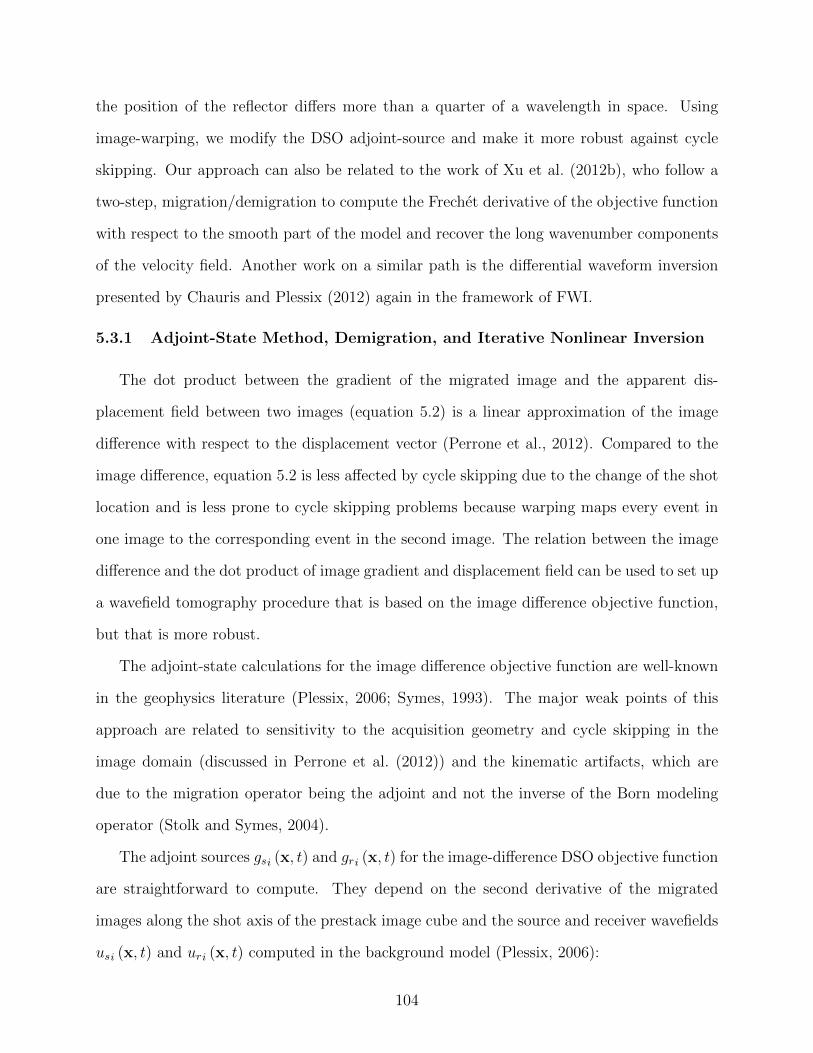
the position of the reflector differs more than a quarter of a wavelength in space. Using
image-warping, we modify the DSO adjoint-source and make it more robust against cycle
skipping. Our approach can also be related to the work of Xu et al. (2012b), who follow a
two-step, migration/demigration to compute the Frechet derivative of the objective function
with respect to the smooth part of the model and recover the long wavenumber components
of the velocity field. Another work on a similar path is the differential waveform inversion
presented by Chauris and Plessix (2012) again in the framework of FWI.
5.3.1 Adjoint-State Method, Demigration, and Iterative Nonlinear Inversion
The dot product between the gradient of the migrated image and the apparent dis-
placement field between two images (equation 5.2) is a linear approximation of the image
difference with respect to the displacement vector (Perrone et al., 2012). Compared to the
image difference, equation 5.2 is less affected by cycle skipping due to the change of the shot
location and is less prone to cycle skipping problems because warping maps every event in
one image to the corresponding event in the second image. The relation between the image
difference and the dot product of image gradient and displacement field can be used to set up
a wavefield tomography procedure that is based on the image difference objective function,
but that is more robust.
The adjoint-state calculations for the image difference objective function are well-known
in the geophysics literature (Plessix, 2006; Symes, 1993). The major weak points of this
approach are related to sensitivity to the acquisition geometry and cycle skipping in the
image domain (discussed in Perrone et al. (2012)) and the kinematic artifacts, which are
due to the migration operator being the adjoint and not the inverse of the Born modeling
operator (Stolk and Symes, 2004).
The adjoint sources gsi (x, t) and gri (x, t) for the image-difference DSO objective function
are straightforward to compute. They depend on the second derivative of the migrated
images along the shot axis of the prestack image cube and the source and receiver wavefields
usi (x, t) and uri (x, t) computed in the background model (Plessix, 2006):
104

gsi = (Ri−1 − 2Ri +Ri+1)uri (5.5)
gri = (Ri−1 − 2Ri +Ri+1)usi. (5.6)
The functions in equation 5.5 and 5.6 are the force terms for the adjoint wave-equations
L (m) asi = gsi (5.7)
L (m) ari = gri, (5.8)
where asi (x, t) and ari (x, t) are the adjoint wavefields and L (m) is the d’Alembert operator.
The adjoint sources generate the scattered fields due to the reflectivity perturbation repre-
sented by (Ri−1 − 2Ri +Ri+1). These wavefields can also be interpreted as the demigrated
reflectivity perturbation (Ri−1 − 2Ri +Ri+1). The gradient of the objective function is then
the zero-lag time correlation of the background and adjoint wavefields (Fichtner et al., 2006;
Plessix, 2006).
By inspecting equations 5.5 and 5.6, we can immediately see the practical issues of
implementing waveform tomography by minimizing the energy of the image difference. Cycle
skipping may arise when the velocity model is severely inaccurate because different images
map the same structures at inconsistent positions in the subsurface.
We propose to replace the term (Ri−1 − 2Ri +Ri+1) in the expression of the adjoint
sources with an approximation derived from image-warping. The apparent displacement field
removes the cycle skipping problem by warping one image into its neighbor. Let us indicate
with u−i and u+i the apparent displacement fields that warp Ri into Ri−1 and Ri into Ri+1,
respectively. Notice that the reference image Ri is the same for the two displacement vector
fields: this is important to obtain smooth sensitivity kernels and avoid cycle skipping. We
can construct approximations of the image differences by computing the dot product of the
image gradient with the displacement fields (Perrone et al., 2012). In order to guarantee
symmetry with respect to the ith shot, we use Ri to construct the image perturbations
105

∆R−i = Ri−1 −Ri ≈ ∇Ri · u−i (5.9)
∆R+i = Ri+1 −Ri ≈ ∇Ri · u+
i . (5.10)
Using the expressions in equations 5.9 and 5.10, we can approximate the second derivative
along the shot axis as follows:
Ri−1 − 2Ri +Ri+1 ≈ ∆R−i + ∆R+i , (5.11)
which is robust against cycle skipping because only one image Ri enters the expression of
the image perturbation.
5.4 Numerical Examples
We test image-warping wavefield tomography for different depths of the reflecting inter-
face and compare it with the direct image difference tomography approach (Plessix, 2006;
Symes, 1993) and local image correlation wavefield tomography (Perrone and Sava, 2012b).
We show that image-warping wavefield tomography is more robust with respect to the depth
of the reflector (i.e. the ratio between the source receiver offset and the depth of the reflector)
and leads to more stable gradients for a model update. We also show how the method fails
to produce sensible gradients in highly refractive media, despite the fact that the objective
function is able to identify the correct model. In this later case, the displacement estimation
is stable but the artifacts in the migrated image lead to spurious scattered wavefields and
artifacts in the sensitivity kernel. Finally, we test our method on the Marmousi model.
5.4.1 Horizontal Reflector
Let us consider a flat horizontal reflector in a homogeneous velocity model. In the
first case, the interface is at 2 km depth and it is due to a density contrast. In order
to measure errors in the velocity model, we analyze two nearby shots: the shot position
of the first shot is x = 3.8 km and the distance between the shots is 200 m. We apply
different homogeneous perturbations to the model and we compute sensitivity kernels using
106

using image-warping wavefield tomography and differential semblance. Figure 5.1 shows the
(a) (b)
(c) (d)
(e) (f)
Figure 5.1: Sensitivity kernels obtained from a deep interface using image-warping wavefieldtomography for (a) high, (c) correct, and (e) low velocities, and using differential semblancewavefield tomography for (b) high, (d) correct, and (f) low velocities.
comparison of the sensitivity kernels for 3 migration models. The rows of Figure 5.1 are, from
top to bottom, kernels for a high, the correct, and a low migration velocity; the columns,
from left to right, show the results using image-warping or standard differential semblance
based on image difference. Image-warping resolves the cycle skipping between the migrated
images that causes the strong sidelobes in differential semblance. Using image-warping to
modify the expression of the adjoint source of differential semblance, we obtain very smooth
sensitivity kernels that correctly represent the perturbation in the velocity model. Figure 5.2
compares the sensitivity analysis performed using the image-warping approximation of the
image difference and standard differential semblance. Notice that in Figure 5.2(a) we observe
107
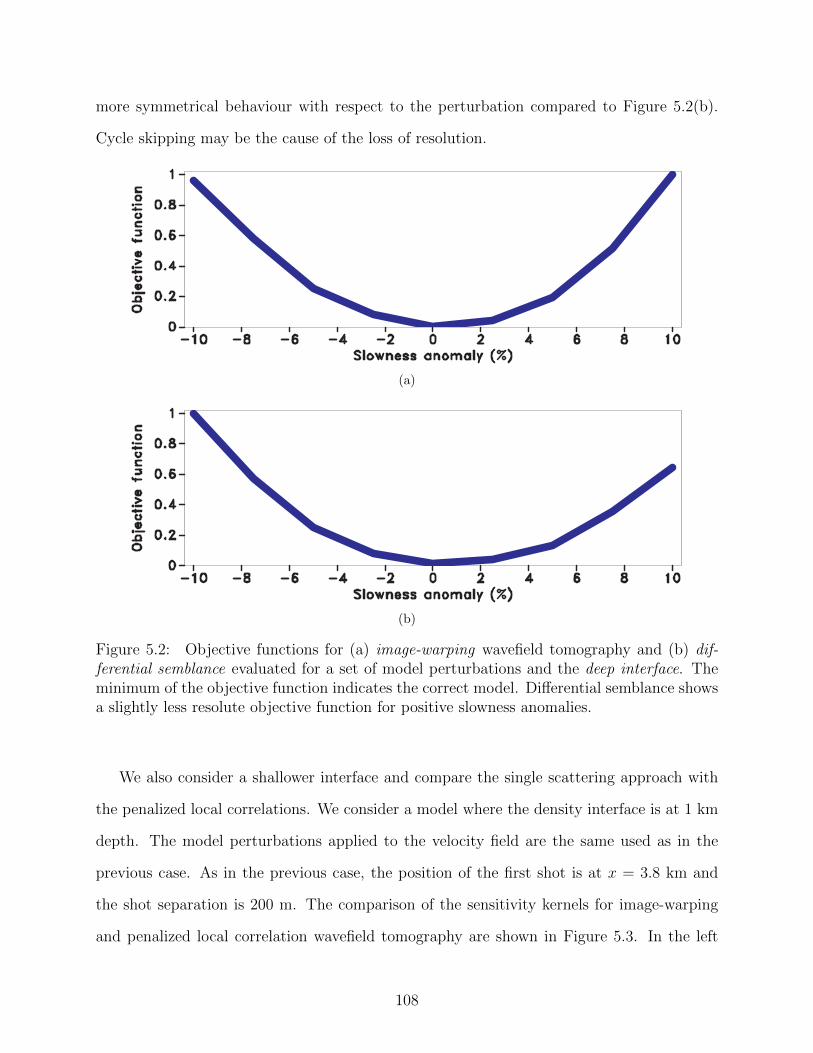
more symmetrical behaviour with respect to the perturbation compared to Figure 5.2(b).
Cycle skipping may be the cause of the loss of resolution.
(a)
(b)
Figure 5.2: Objective functions for (a) image-warping wavefield tomography and (b) dif-ferential semblance evaluated for a set of model perturbations and the deep interface. Theminimum of the objective function indicates the correct model. Differential semblance showsa slightly less resolute objective function for positive slowness anomalies.
We also consider a shallower interface and compare the single scattering approach with
the penalized local correlations. We consider a model where the density interface is at 1 km
depth. The model perturbations applied to the velocity field are the same used as in the
previous case. As in the previous case, the position of the first shot is at x = 3.8 km and
the shot separation is 200 m. The comparison of the sensitivity kernels for image-warping
and penalized local correlation wavefield tomography are shown in Figure 5.3. In the left
108

(a) (b)
(c) (d)
(e) (f)
Figure 5.3: Sensitivity kernels obtained from a shallow interface using image-warping wave-field tomography for (a) high, (c) correct, and (e) low velocities, and using penalized localcorrelations wavefield tomography for (b) high, (d) correct, and (f) low velocities. Penalizedlocal correlation are strongly biased at the edges of the subsurface aperture.
109

column, image-warping shows the ability to return kernels with the correct sign even when
the interface is close to the surface, and cycle skipping problems are enhanced because
the difference between the apertures of the two shots increases. Penalized local correlations
suffer from the strong bias at the edges of the aperture, where the two images do not overlap.
The comparison of the objective functions for different values of the model perturbation in
(a)
(b)
Figure 5.4: Objective functions for (a) image-warping wavefield tomography and (b) penal-ized local correlations evaluated for a set of model perturbations and the shallow interface.Penalized local correlation fail to identify the correct model.
Figure 5.4 highlights a strong bias for the penalized local correlations when the reflecting
interface is shallow and the ratio between the depth of the interface and the shot separation
is small. Nonetheless, the gradients obtained using image-warping for a deeper interface are
comparable with the results reported in Perrone and Sava (2012b) for the objective function
110
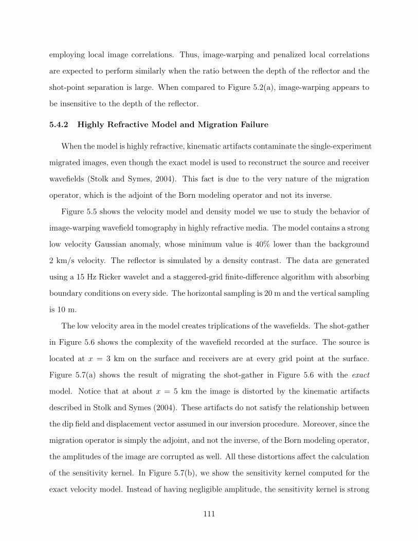
employing local image correlations. Thus, image-warping and penalized local correlations
are expected to perform similarly when the ratio between the depth of the reflector and the
shot-point separation is large. When compared to Figure 5.2(a), image-warping appears to
be insensitive to the depth of the reflector.
5.4.2 Highly Refractive Model and Migration Failure
When the model is highly refractive, kinematic artifacts contaminate the single-experiment
migrated images, even though the exact model is used to reconstruct the source and receiver
wavefields (Stolk and Symes, 2004). This fact is due to the very nature of the migration
operator, which is the adjoint of the Born modeling operator and not its inverse.
Figure 5.5 shows the velocity model and density model we use to study the behavior of
image-warping wavefield tomography in highly refractive media. The model contains a strong
low velocity Gaussian anomaly, whose minimum value is 40% lower than the background
2 km/s velocity. The reflector is simulated by a density contrast. The data are generated
using a 15 Hz Ricker wavelet and a staggered-grid finite-difference algorithm with absorbing
boundary conditions on every side. The horizontal sampling is 20 m and the vertical sampling
is 10 m.
The low velocity area in the model creates triplications of the wavefields. The shot-gather
in Figure 5.6 shows the complexity of the wavefield recorded at the surface. The source is
located at x = 3 km on the surface and receivers are at every grid point at the surface.
Figure 5.7(a) shows the result of migrating the shot-gather in Figure 5.6 with the exact
model. Notice that at about x = 5 km the image is distorted by the kinematic artifacts
described in Stolk and Symes (2004). These artifacts do not satisfy the relationship between
the dip field and displacement vector assumed in our inversion procedure. Moreover, since the
migration operator is simply the adjoint, and not the inverse, of the Born modeling operator,
the amplitudes of the image are corrupted as well. All these distortions affect the calculation
of the sensitivity kernel. In Figure 5.7(b), we show the sensitivity kernel computed for the
exact velocity model. Instead of having negligible amplitude, the sensitivity kernel is strong
111

(a)
(b)
Figure 5.5: (a) Velocity model used to study the behavior of the inversion in highly refractingmedia. The low velocity anomaly is Gaussian-shaped and its minimum value is 40% lowerthan the 2 km/s background. (b) Density model used to generate reflections.
112

Figure 5.6: Shot-gather for a source at x = 3 km. Notice the complicated response of themedium due to the triplications of the wavefield passing through the low velocity anomaly.
and totally spurious.
Figure 5.8 shows the objective function obtained by perturbing the correct model with
a Gaussian anomaly that progressively cancels out the low velocity zone. Interestingly,
although the sensitivity kernel is inaccurate, the objective function is still able to measure
the distance from the correct model. This indicates that although the velocity error measure
is efficient, the linearizations used for computing the sensitivity kernels and model update
can introduce strong errors.
5.4.3 Marmousi Model
We also test our approach on the Marmousi model (Figure 5.9(a)). We model 100 shots
separated by 80 m. The spatial sampling is 8 m in both the x and z direction. Receivers are
located at every grid point on the surface. The data are modeled without free-surface multi-
ples but internal multiples are present in the data. We assume that free-surface multiples can
be effectively removed from the data using SRME (Verschuur, 1991). The Marmousi model
represents a complex land-like scenario and is characterized by multipathing and strong re-
113

(a)
(b)
Figure 5.7: Migrated image obtained from the shot-gather in Figure 5.6 with the correctvelocity model. Observe the distorted image of the reflectors and the artifacts introducedby the migration operator. (b) Sensitivity kernel obtained using image-warping wavefieldtomography for the correct velocity model. The kernel should be very small and incoherentbecause the model is actually correct; the spurious kernel is thus completely due to theartifacts in the image.
114
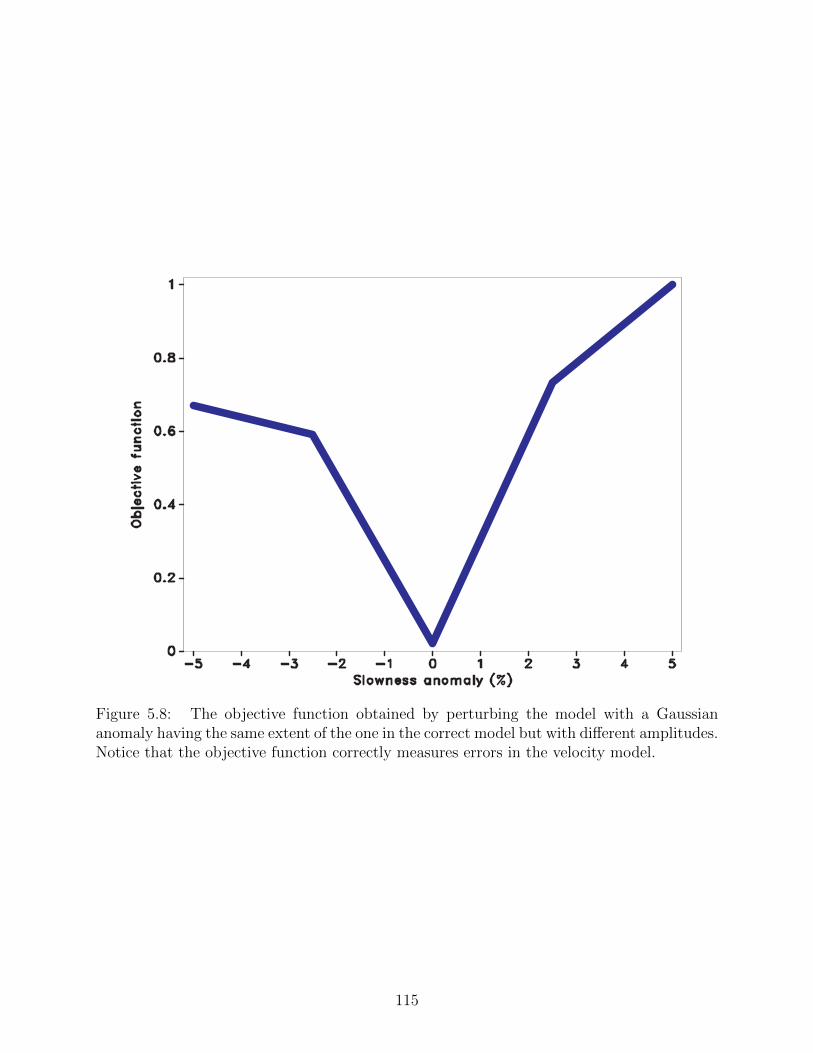
Figure 5.8: The objective function obtained by perturbing the model with a Gaussiananomaly having the same extent of the one in the correct model but with different amplitudes.Notice that the objective function correctly measures errors in the velocity model.
115

fractions. This complexity is exemplified by the raypaths calculated in a smoothed version
of the correct model (Figure 5.9(b)) for a shot at x = 4.8 km.
Figure 5.10 shows the preprocessing applied to the shot gathers before imaging and
inversion. In Figure 5.10(a), we display the shot-gather for a source located at x = 1.6 km
after removal of the direct arrival. In order to balance the amplitude of the reflection events
and of the reflectors in the image, we equalized each trace by scaling them by a smooth local
estimate of the rms value along the trace itself. Figure 5.10(b) shows the result of applying
the amplitude equalization to the shot-gather in Figure 5.10(a) and then smoothly muting
the refracted energy. Notice that the later arrival are much more visible after the amplitude
equalization.
The initial model is the vertical gradient of velocity in Figure 5.11(a). The velocity
increases 0.5 km/s with depth and is generally slower than in the correct model. The migrated
image obtained using this model is shown in Figure 5.11(b). The central part of the image
is non interpretable and all reflectors are mispositioned and defocused; the deep and strong
reflectors are shifted about 500 m upward. The noise in the image is due to the strong errors
in the migration model and the inconsistent imaging of the reflectors from different shots.
Also, the internal multiples in the data are not imaged correctly since migration is based on
single-scattering (Born) assumptions. The complex wave propagation, the strong refractions,
and the the internal multiples contribute noise and artifacts in the migrated image. For
example, at x = 1 km and z = 2.7 km ghost reflectors due to strong internal multiples can
be observed, and in the central part of the model, at x = 4.5 and z = 2 km, the unfocused
events do not combine constructively and lead to random noise rather than an image of the
geologic structures. In the latter case, the complexity of the faulted portion of the model
creates scattering that is not correctly remapped using the initial model in Figure 5.11(a).
These artifacts are the main source of noise for our wavefield tomography approach since they
do not carry information about specular reflections and since they decrease the reliability
of the estimated displacement vector field, and thus of the adjoint sources. By analyzing
116
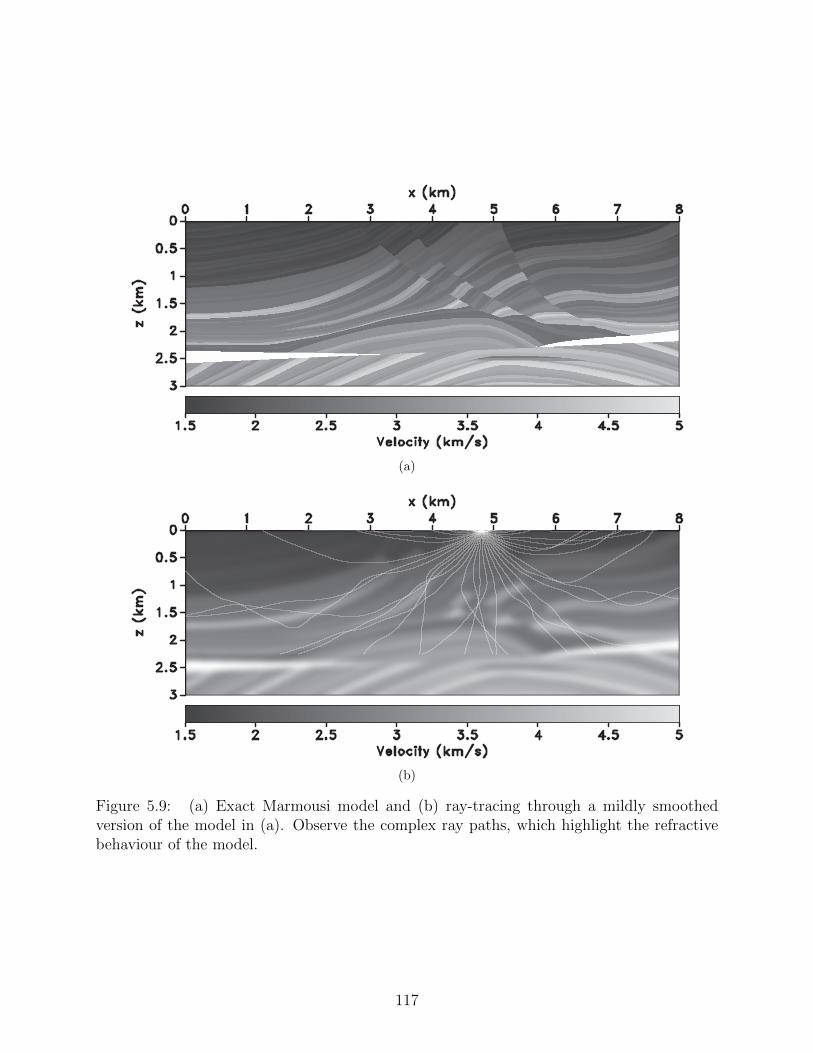
(a)
(b)
Figure 5.9: (a) Exact Marmousi model and (b) ray-tracing through a mildly smoothedversion of the model in (a). Observe the complex ray paths, which highlight the refractivebehaviour of the model.
117
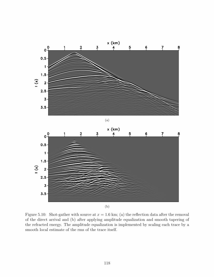
(a)
(b)
Figure 5.10: Shot-gather with source at x = 1.6 km; (a) the reflection data after the removalof the direct arrival and (b) after applying amplitude equalization and smooth tapering ofthe refracted energy. The amplitude equalization is implemented by scaling each trace by asmooth local estimate of the rms of the trace itself.
118
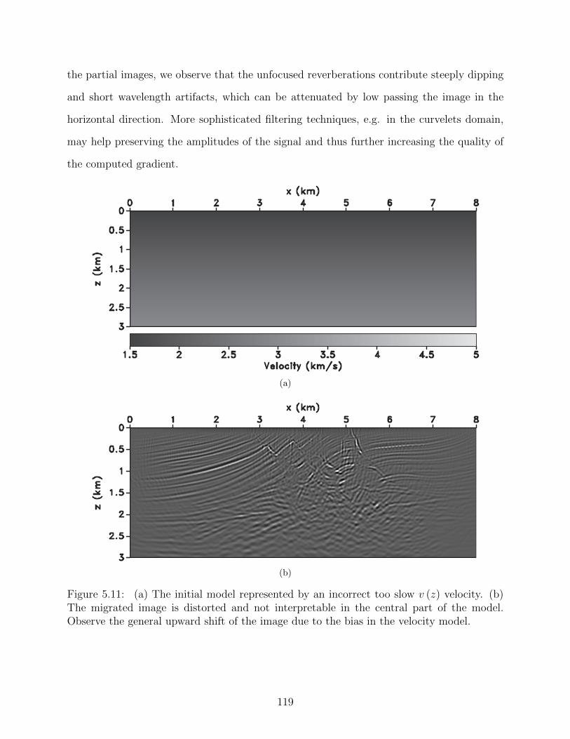
the partial images, we observe that the unfocused reverberations contribute steeply dipping
and short wavelength artifacts, which can be attenuated by low passing the image in the
horizontal direction. More sophisticated filtering techniques, e.g. in the curvelets domain,
may help preserving the amplitudes of the signal and thus further increasing the quality of
the computed gradient.
(a)
(b)
Figure 5.11: (a) The initial model represented by an incorrect too slow v (z) velocity. (b)The migrated image is distorted and not interpretable in the central part of the model.Observe the general upward shift of the image due to the bias in the velocity model.
119
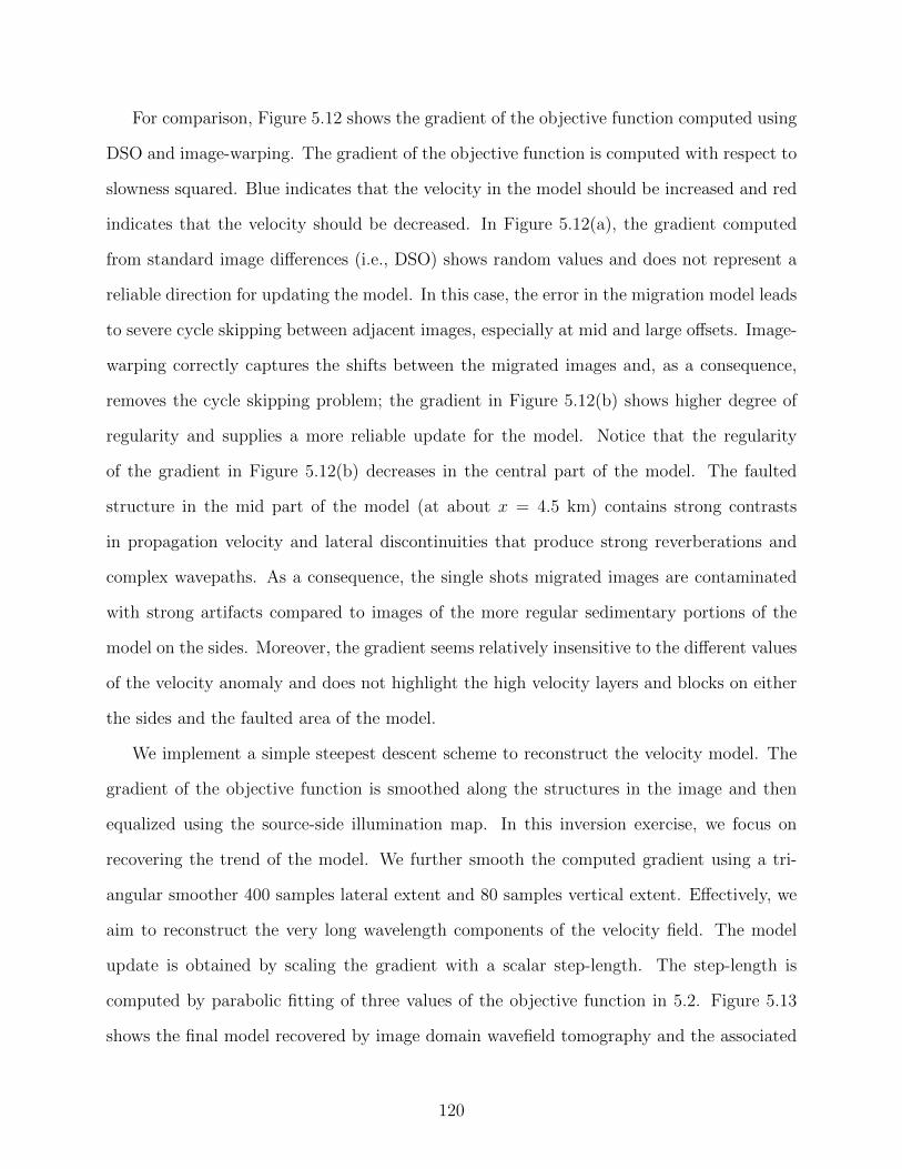
For comparison, Figure 5.12 shows the gradient of the objective function computed using
DSO and image-warping. The gradient of the objective function is computed with respect to
slowness squared. Blue indicates that the velocity in the model should be increased and red
indicates that the velocity should be decreased. In Figure 5.12(a), the gradient computed
from standard image differences (i.e., DSO) shows random values and does not represent a
reliable direction for updating the model. In this case, the error in the migration model leads
to severe cycle skipping between adjacent images, especially at mid and large offsets. Image-
warping correctly captures the shifts between the migrated images and, as a consequence,
removes the cycle skipping problem; the gradient in Figure 5.12(b) shows higher degree of
regularity and supplies a more reliable update for the model. Notice that the regularity
of the gradient in Figure 5.12(b) decreases in the central part of the model. The faulted
structure in the mid part of the model (at about x = 4.5 km) contains strong contrasts
in propagation velocity and lateral discontinuities that produce strong reverberations and
complex wavepaths. As a consequence, the single shots migrated images are contaminated
with strong artifacts compared to images of the more regular sedimentary portions of the
model on the sides. Moreover, the gradient seems relatively insensitive to the different values
of the velocity anomaly and does not highlight the high velocity layers and blocks on either
the sides and the faulted area of the model.
We implement a simple steepest descent scheme to reconstruct the velocity model. The
gradient of the objective function is smoothed along the structures in the image and then
equalized using the source-side illumination map. In this inversion exercise, we focus on
recovering the trend of the model. We further smooth the computed gradient using a tri-
angular smoother 400 samples lateral extent and 80 samples vertical extent. Effectively, we
aim to reconstruct the very long wavelength components of the velocity field. The model
update is obtained by scaling the gradient with a scalar step-length. The step-length is
computed by parabolic fitting of three values of the objective function in 5.2. Figure 5.13
shows the final model recovered by image domain wavefield tomography and the associated
120
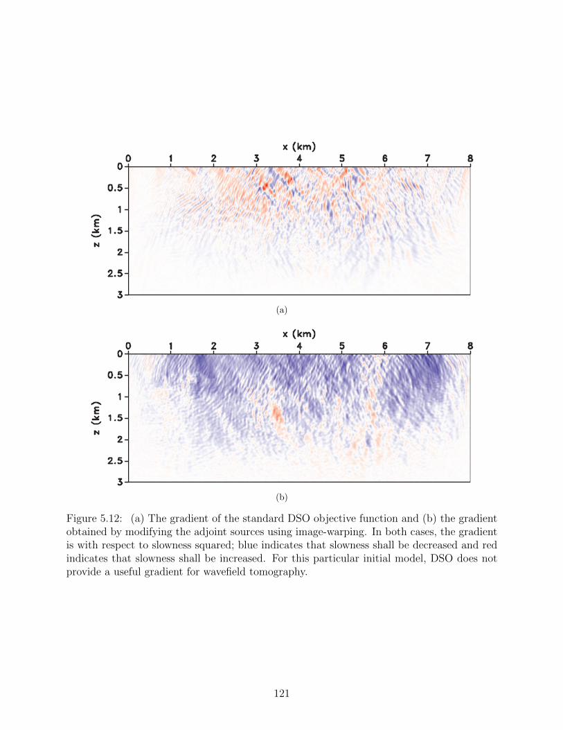
(a)
(b)
Figure 5.12: (a) The gradient of the standard DSO objective function and (b) the gradientobtained by modifying the adjoint sources using image-warping. In both cases, the gradientis with respect to slowness squared; blue indicates that slowness shall be decreased and redindicates that slowness shall be increased. For this particular initial model, DSO does notprovide a useful gradient for wavefield tomography.
121
migrated image. The inversion reconstructs the very smooth background velocity model in
Figure 5.13(a), which is characterized by a steeper velocity gradient than the initail model
in Figure 5.11(a). By comparing the exact model in Figure 5.9(a) and the final image in Fig-
ure 5.13(b), we can see that image-warping wavefield tomography is able to better position
reflectors where the geology is relatively simple and the geometrical features of the image
can be measured more precisely. In the shallower part of the model, the truncation of the
sediments against the faults is now better interpretable (e.g. x = 3.5 km and z = 1.0 km
and along the fault that reaches the surface at about x = 5.0 km). However, the quality of
the image in the central, faulted portion of the model, because of the high level of coherent
noise in the partial images, is quickly decreases.
Figure 5.14 shows that the objective function decreases smoothly and monotonically but
the convergence slows down after about 50 iterations. The nonzero value of the objective
function is mainly due to migration artifacts, whose contribution becomes significant with
respect to the shifts measured on actual reflectors.
Finally, we used the model reconstructed by image-warping wavefield tomography as
the initial guess for data-domain full-waveform inversion. Figure 5.15 shows the final re-
constructed model after 60 iterations of full-waveform inversion. The data used for the
data-domain inversion test are the low-passed filtered version of the data used for image-
domain tomography; the cut-off frequency is 3 Hz. Full-waveform inversion converges to a
high-resolution result and reconstructs high-wavenumber features of the model. Compared
to the actual Marmousi model in Figure 5.9(a), we were able to accurately reconstruct the
geology in the central part of the model and up to a depth of about 2.5 km. The quality
of the result comes from the correct kinematics of the wavefields in the sedimentary part
of the model, which was reconstructed by image-warping wavefield tomography and allows
one to correctly position the reflectors. Image-warping tomography recovers the very low
wavenumber components of the velocity model, which are crucial to avoid cycle-skipping in
data-domain inversion. The deeper part of the model, below 2.5 km, is poorly constrained
122
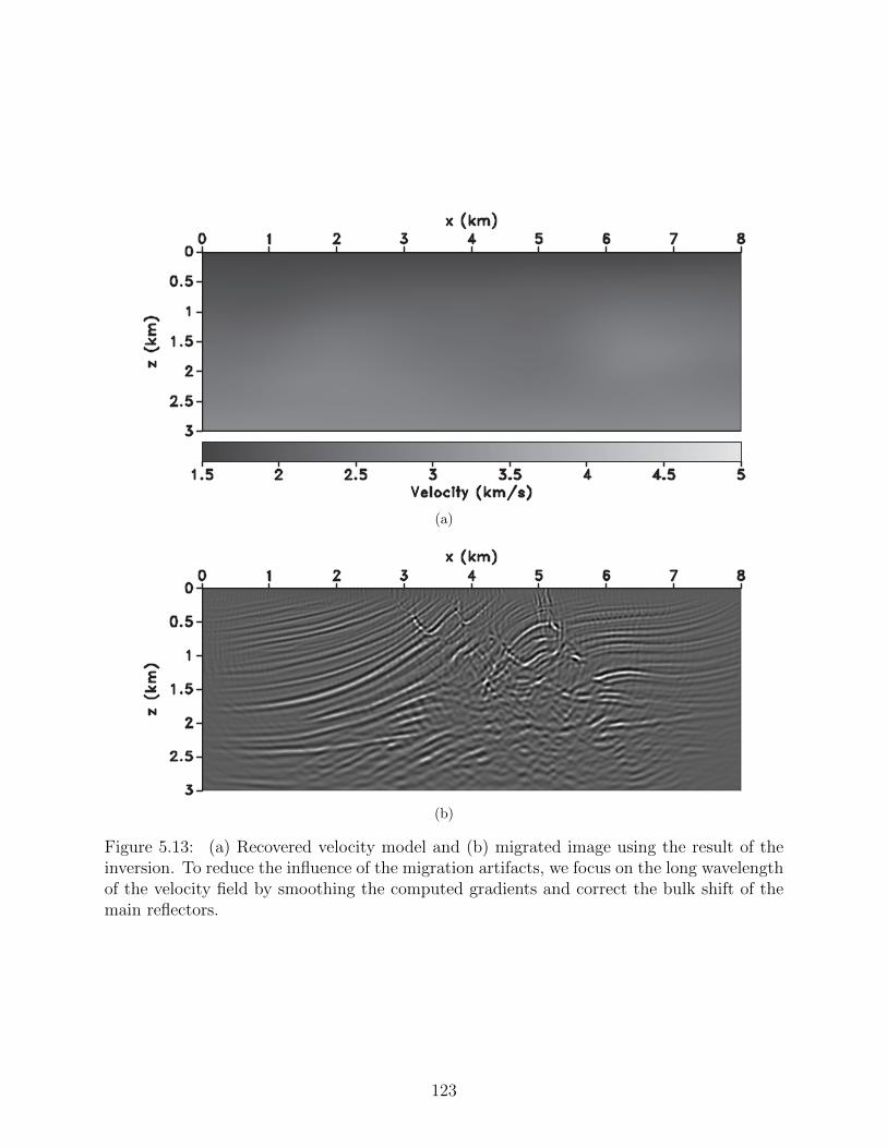
(a)
(b)
Figure 5.13: (a) Recovered velocity model and (b) migrated image using the result of theinversion. To reduce the influence of the migration artifacts, we focus on the long wavelengthof the velocity field by smoothing the computed gradients and correct the bulk shift of themain reflectors.
123

Figure 5.14: The value of the objective function decreases smoothly with iterations. Conver-gence slows down after 50 iterations because the residuals measured on migration artifactsbecomes significant with respect to the residual measured on actual reflectors.
Figure 5.15: Full-waveform inversion result obtained using the image-warping wavefieldtomography inverted model in Figure 5.13(a) as initial guess. The data are low-passedfiltered with cut-ff frequency of 3 Hz. The improved kinematics of the model obtained byimage-warping wavefield tomography removes the cycle-skipping problem in the data domainand allows one to reconstruct a high-resolution model.
124

by the data. Image-warping wavefield tomography is not able to correct the velocity gradient
and consequently the quality of the data-domain inversion is lower, as well.
5.5 Discussion
The image difference objective function proposed by Symes (1993) and Plessix (2006) as
a regularization term for full-waveform inversion is simple to implement and carries straight-
forward physical intuition about the action of the inversion. In media that are not strongly
refractive, cycle skipping can be effectively and efficiently avoided using the apparent dis-
placement field between migrated images and constructing robust approximations of image
differences. Estimating the displacement field and computing the image gradient have a
negligible computational cost compared to migration. Moreover, we preserve the physical
interpretation of the image perturbation that enters the expression of the adjoint sources
in equations 5.5 and 5.6, which is useful for quality control and for quickly assessing the
evolution of the inversion result. The residual evaluation is immediate and the calculation of
the adjoint sources is straightforward compared to local correlation waveform tomography,
where the computation of the adjoint-sources requires nonstationary convolutions between
the migrated images and the penalty operators followed by local scaling by the background
wavefields. When compared to methods that require image-gathers or extended images,
image-warping wavefield tomography appears easier to implement and less computation-
ally demanding. On the other hand, by stacking contributions from different experiments,
methods based on image-gathers are intrinsically less sensitive to random noise and can also
attenuate the migration operator noise.
The adjoint-state calculations for the objective function in equation 5.2 are computa-
tionally expensive and involved. In appendix A, we show that not only the background
wavefields but also their spatial derivatives are required. Moreover, the warping field re-
quires a dedicated procedure based on connective functions, which link the warping vectors
to the velocity model, and this more complicated procedure would not remove the sensitivity
to migration artifacts. From an inversion perspective, this step increases the dimensionality
125
of the problem; Luo and Schuster (1991) operate on scalar shifts whereas we manipulate
vectors defined at every point in the discretized space. A further difference between image
and data domain is the presence (or lack thereof) of artifacts. The data represent the ground
truth that we want to match, whereas the single migrated images are contaminated by the
migration operator noise. Because of this, the data domain appear to be more suitable
for measuring shifts between waveforms than the image domain. On the other hand, the
most reliable information about traveltimes comes from transmitted and refracted waves,
which can be missing depending on the model and/or acquisition design. In this second
case, measuring relative shifts in the image domain can still supply valuable information for
reconstructing the velocity field.
Computing the relative shift between two images in local seamlessly overlapping windows
requires some degree of overlapping of the two migrated images. The quantity of interest
to qualitatively characterize the distance between the two images in simple subsurface ge-
ometries is the ratio between the shot-point separation and the depth of the reflectors. The
smaller this ratio, the greater the overlap between migrated images. When we estimate the
shift between the migrated images using penalized local correlations, the extent of the local
window constrains the domain in which the maximum of the correlation must be. When the
separation between the shot is large and the local window is not wide enough to capture the
position of the maximum of the local correlation, we introduce an error in the evaluation
of the residuals. Notice that increasing the size of the local correlation window implies a
decrease in resolution. Moreover, if other events (more reflectors) enter the local window
and/or the reflector changes orientation in space, increasing the extent of the local window
implies a drop in the values of the estimated correlation coefficients and thus a decrease in
the quality of the estimated shifts. The displacement vector field is more robust than the
penalized local correlations because of the iterative search and warping procedure used (Hale
et al., 2008) and thus it allows us to obtain high-quality velocity updates at shallow depths
where the ratio between the shot distance and the depth of the reflector is relatively high.
126
The main drawback of performing inversion in the shot-migrated image domain is related
to the nature of the migration operator and to the associated migration artifacts. In highly
refractive media, triplications and multipathing between source and receiver produce artifacts
in the migrated image (Stolk and Symes, 2004). The artifacts are due to the migration
operator being the adjoint and not the inverse of the Born modeling operator; they have the
same frequency content of the signal and, although stacking over experiments removes them
from the final image, they severely contaminate the migrated images for individual shots.
These kinematic artifacts represent the principal source of noise for our method: they do not
satisfy the assumed relation between the directions of the image gradient and displacement
vector field; moreover they introduce events with conflicting dips in the image that make
the estimation of the displacement field noisier. Least-square migration (Nemeth et al.,
1999) may be a possible solution in the case of white Gaussian noise but would increase the
computational cost and time. Unfortunately, migration artifacts do not follow a Gaussian
distribution and thus least-squares migration is ineffective in removing migration artifacts
from single-shot images.
A substantial difference of image-warping wavefield tomography with respect to methods
based on extended images (Shen and Symes, 2008; Yang and Sava, 2011a), which involve all
shots in the construction of the adjoint sources, is the fundamentally different tomographic
behaviour. As described in Vasconcelos et al. (2010), extended images represent the reflec-
tion response for virtual sources constructed in the subsurface at specific locations through
interferometry. These sources illuminate a wide range of directions and thus the sensitivity
kernels obtained from each point have a wide spatial spectral content. On the contrary, our
method (and conventional differential semblance in the shot-domain) constructs the adjoint
sources from single images, each of which is illuminated from a very limited range of direc-
tion. The poor illumination of the model that individual images supply reflects in extremely
smooth sensitivity kernels that do not capture high wavenumber features in the model.
127

In complicated models, such as the Marmousi model, regularization plays an important
role in balancing the strength of the update and removing the natural bias that comes from
the uneven illumination and the complexity of the subsurface structures. The smoothness
and regularity of the estimated displacement vector field is also very important since it
controls the quality of the adjoint sources and the smoothness of the sensitivity kernels.
Nonetheless, image-warping wavefield tomography appears to be characterized by smooth
gradients that can be used to easily correct substantial errors in the velocity models and
then to bootstrap or regularize velocity analysis schemes that supply higher resolution.
5.6 Conclusions
The image-difference objective function for wavefield tomography in the migrated-shot
domain can be made more robust using image-warping. The displacement vector field that
warps a migrated image into the image obtained from a neighboring experiment removes
cycle-skipping because every reflector in one image is mapped into the corresponding event
in the second image.
Our method is more effective than local image correlation wavefield tomography for shal-
low reflectors, i.e., when the ratio between the source separation and the depth of the reflector
is high. However, kinematic artifacts contaminate the image in highly refractive media and
destabilize the computation of the sensitivity kernel. Nonetheless, in non-pathological cases,
the image-warping objective function can measure the distance between different models and
identify the most coherent images, thus enabling local gradient-based optimization.
An inversion test on the Marmousi model shows that image-warping wavefield tomogra-
phy is able to correct strong errors in the velocity model where the geometry of the reflectors
is relatively simple and regular. Although kinematic artifacts in the single shot migrated
images prevent a successful inversion in complex areas, the correct reconstruction of the
very low wavenumber components of the model makes it possible to use the result of image-
warping wavefield tomography as an initial model for higher-resolution techniques and to
avoid cycle-skipping in the data-domain.
128

5.7 Acknowledgments
This work was supported by the sponsors of the Consortium Project on Seismic Inverse
Methods for Complex Structures. The reproducible numerical examples in this paper use
the Madagascar open-source software package freely available from http://www.ahay.org and
the Mines JTK freely available at https://github.com/dhale/jtk.
129
CHAPTER 6
CONCLUSIONS AND SUGGESTIONS
6.1 Main Conclusions
Conventional shot-domain common-image gathers are not suitable for migration velocity
analysis because they are affected more than other gathers by the noise of the migration
operator, i.e. the migration artifacts that contaminate the single shot image. Even when
the model is not highly refractive, if the velocity error is strong, differential semblance
optimization produces low quality gradients due to cycle skipping between the migrated
images. Image-warping removes the problem of cycle skipping in a natural and intuitive way
with minimum computational cost.
6.1.1 Image-Warping and Differential Semblance
In Chapter 2, I show the connection between the image difference and image-warping
using a Taylor expansion of the image with respect to the estimated apparent displacement
vector field. The displacement vectors map each point in a reference image to the corre-
sponding point in a second image and describe the warping transformation that links the
two images. The warping vector field allows one to design an image perturbation that can
be linked to the perturbation in the migration model via a linearized operator obtained from
the one-way downward continuation operator used in migration.
6.1.2 Geometrical Relationship between Structural Information and Warping
The warping vector field encodes the apparent displacement between migrated images.
The approximation derived in Chapter 2 links the image difference, the gradient of the
migrated image, and the warping field. In particular, the approximation highlights the
geometrical relation that the warping vector and the dip of locally planar events must satisfy
when the migration model accurately describes the wave kinematics.
130

Errors in the velocity model introduce a component in the warping field that is aligned
with the dip of the reflector. In Chapter 3, I developed a measure of the normal component
of the apparent shift using penalized local correlations. This approach allows me to design
an optimization problem that does not rely on linearizations of the wave propagation and
migration operators. In particular, it allows me to include a two-way wave propagation
operator in the inversion and thus integrates reverse-time migration in the velocity estimation
procedure.
6.1.3 Inversion of Apparent Displacements in the Image Domain
In Chapters 3 and 4, I show how to measure and successfully invert apparent displace-
ments between neighboring shot-gathers in the image domain. I implemented a wavefiled
tomography algorithm that can be used for velocity model building, in the context of mi-
gration velocity analysis, and for monitoring changes in a reservoir under depletion, in the
context of 4D time-lapse seismic. This approach exploits the local coherency of the reflectors
in the image domain to balance either the poor quality of the gather or the lack of data in
the shot direction and allows one to reconstruct anomalies in the migration model from a
minimum number of shot gathers.
6.1.4 Superiority of Warping Vectors over Penalized Correlations
In Chapter 5, I point out the deficiencies of penalized local correlations and use the
warping relations between migrated images (Chapter 2) to make the conventional differential
semblance optimization in the shot-domain robust against cycle-skipping and differences in
the shot aperture. In contrast to the algorithm presented in Chapter 2, in Chapter 5 I
used a two-way wave propagation operator. Image-warping wavefield tomography produces
smooth sensitivity kernels that easily reconstruct the very long wavelength components of
the velocity model with negligible additional computational cost with respect to conventional
differential semblance optimization.
131
6.2 Future Research and Suggestions
In this thesis, I focused on 2D tomography and used crosscorrelation measures to estimate
displacements and vector fields. Here, I would like to suggest some direction for future
research and development.
6.2.1 Artifact-free Migration Algorithm
Seismic migration is mathematically defined as the adjoint of a foward single-scattering
Born modeling operator. If the complexity of the model is such that the forward operator
is not diagonal or diagonally dominant, the application of the adjoint operator to the data
introduces coherent noise in single experiment images. These artifacts are the main source of
noise for my approach since they do not satisfy the geometrical relations between the warping
and dip vector field. The development of an imaging algorithm capable of migrating single
experiments without introducing migration artifacts would greatly improve the quality of
the inversion.
6.2.2 Warping Vector Field Calculation
My inversion approach relies on the accurate estimation of the relative displacements
between migrated images. The vector displacements, which are a more robust measure of
shifts than penalized local correlations, are also based on local correlations and are subject
to the noise introduced by migration artifacts as well. Techniques based on the solution
of a global optimization problem, e.g. dynamic image-warping, are likely to produce higher
quality estimates of the displacement field. A more robust estimation of the warping field can
be beneficial for further improving the quality of the sensitivity kernels and for increasing
the resolution of the inversion. Although a direct multidimensional estimation of vector
displacements using dynamic image-warping would be computationally very expensive, one
can measure one-dimensional shifts along the coordinate axes, warp the input signal, and
thus iteratively build the total vector displacement field. This approach is analogous to the
procedure implemented for local image correlations and is computationally efficient.
132

6.2.3 Bi-objective FWI/MVA Optimization
Shot-domain gathers are naturally produced by many migration algorithms, in particular
reverse-time migration, without any extra computational cost. Reverse-time migration (up
to the appropriate scaling) is the gradient of full-waveform inversion. A velocity analysis
approach that effectively uses the information contained in the partial contributions coming
from each individual experiment represents an ideal regularization approach to control the
long wavenumber components of the model.
A natural development of this work would be to integrate my image-domain wavefield
tomography algorithm into conventional full-waveform inversion. The image-domain misfit
term represents more than just regularization because it introduces actual information about
the velocity model and not just a priori information about the smoothness of the macro
model.
133

REFERENCES CITED
Aki, K., and P. G. Richards, 2002, Quantitative seismology: University Science Books.
Al-Yahya, K., 1989, Velocity analysis by iterative profile migration: Geophysics, 54, P.718–729.
Albertin, U., P. Sava, J. Etgen, and M. Maharramov, 2006, Adjoint wave-equation velocityanalysis: Presented at the 74th Ann. Internat. Mtg., SEG.
Baysal, E., D. D. Kosloff, and J. W. C. Sherwood, 1983, Reverse time migration: Geophysics,48, 1514–1524.
Biondi, B., and P. Sava, 1999, Wave-equation migration velocity analysis: 69th AnnualInternational Meeting, SEG, Expanded Abstracts, 1723–1726.
Biondi, B., and W. W. Symes, 2004, Angle-domain common-image gathers for migrationvelocity analysis by wavefield continuation imaging: Geophysics, 69, 1283–1298.
Bishop, T. N., K. P. Bube, R. T. Cutler, R. T. Langan, P. L. Love, J. R. Resnick, R. T.Shuey, D. A. Spindler, and H. W. Wyld, 1985, Tomographic determination of velocity anddepth in laterally varying media: Geophysics, 50, 903–923.
Brossier, R., S. Operto, and J. Virieux, 2010, Which data residual norm for robust elasticfrequency-domain full waveform inversion?: Geophysics, 75, R37 – R46.
Bunks, C., F. M. Saleck, S. Zaleski, and G. Chavent, 1995, Multiscale full waveform inversion:Geophysics, 60, 1457–1473.
Carcione, J., 2007, Wave fields in real media wave propagation in anisotropic, anelastic,porous and electromagnetic media: Elsevier. Handbook of Geophysical Exploration.
Chang, W., P. Carrion, and G. Beylkin, 1987, Wavefront sets of solutions to linearised inversescattering problems: Inverse Problems, 3, 683 – 690.
Chauris, H., and R.-E. Plessix, 2012, Investigating the differential waveform inversion: 74thConference and Exhibition, EAGE, Extended Abstracts, Workshops WS06.
Chavent, G., and C. A. Jacewitz, 1995, Determination of background velocities by multiplemigration fitting: Geophysics, 60, 476–490.
134

Claerbout, J. F., 1985, Imaging the earth’s interior: Blackwell Publishing.
Colton, D., and R. Kress, 1998, Inverse acoustic and electromagnetic scattering theory:Springer-Verlag.
de Vries, D., and A. J. Berkhout, 1984, Velocity analysis based on minimum entropy: Geo-physics, 49, 2132–2142.
Dickens, T. A., 1994, Diffraction tomography of crosswell imaging of nearly layered media:Geophysics, 59.
Farmer, P. A., I. F. Jones, H. Zhou, R. I. Bloor, and M. C. Goodwin, 2006, Application ofreverse time migration to complex imaging problems: First Break, 24, 65–73.
Faye, J.-P., and J.-P. Jeannot, 1986, Prestack migration velocity analysis from focusing depthimaging: Presented at the 56th Annual International Meeting, SEG.
Fei, W., and P. Williamson, 2010, On the gradient artifacts in migration velocity analysisbased on differential semblance optimization: 80th Annual International Meeting, SEG,Expanded Abstracts, 4071–4076.
Fichtner, A., H.-P. Bunge, and H.Igel, 2006, The adjoint method in seismology I. theory:Physics of the Earth and Planetary Interiors, 86–104.
Fomel, S., 2002, Applications of plane-wave destruction filters: Geophysics, 67, 1946–1960.
——–, 2011, Theory of 3-d angle gathers in wave-equation imaging: 81st Annual Interna-tional Meeting, SEG, Expanded Abstracts.
Fowler, P., 1985, Migration velocity analysis by optimization: Technical Report 44, StanfordExploration Project.
Fuck, R. F., A. Bakulin, and I. Tsvankin, 2009, Theory of traveltime shifts around com-pacting reservoirs: 3d solutions for heterogeneous anisotropic media: Geophysics, 74,D25–D36.
Gazdag, J., and P. Sguazzero, 1984, Migration of seismic data by phase shift plus interpola-tion: Geophysics, 49.
Girard, A., and I. Vasconcelos, 2010, Image-domain time-lapse inversion with extended im-ages: Presented at the 80th Annual International Meeting, SEG.
Green, A. G., E. Lanz, and H. Maurer, 1998, Refraction tomography over a buried wastedisposal site: Geophysics, 63, 1414–1433.
135

Hale, D., 2006, Fast local cross-correlations of images: 76th Annual International Meeting,SEG, Expanded Abstracts, 3160 – 3164.
——–, 2009, A method for estimating apparent displacement vectors from time-lapse seismicimages: Geophysics, 74, V99 – V107.
Hale, D., B. Cox, and P. J. Hatchell, 2008, Apparent horizontal displacements in time-lapseseismic images: 78th Annual International Meeting, SEG, Expanded Abstracts, 3169–3173.
Hatchell, P. J., and S. J. Bourne, 2005, Measuring reservoir compaction using time-lapsetimeshifts: Presented at the 75th Annual International Meeting, SEG.
Kelly, S., J. R. Martinez, B. Tsimelzon, and S. Crawley, 2010, A comparison of inversionresults for two full-waveform methods that utilize the lowest frequencies in dual-sensorrecordings: Presented at the 80th Annual International Meeting, SEG.
Krebs, J. R., J. E. Anderson, A. Baumstein, S. Lee, R. Neelamani, and M.-D. Lacasse, 2009,Fast full wave seismic inversion using source encoding: Presented at the 79th AnnualInternational Meeting, SEG.
Lambare, G., M. Alerini, R. Baina, and P. Podvin, 2004, Stereotomography: a semi-automatic approach for velocity macromodel estimation: Geophysical Prospecting, 52,671–681.
Larner, K., and V. Celis, 2007, Selective-correlation velocity analysis: Geophysics, 72, U11–U19.
Lions, J., 1972, Nonhomogeneous boundary value problems and applications: Springer Ver-lag, Berlin.
Liu, F., D. W. Hanson, N. D. Whitmore, R. S. Day, and R. H. Stolt, 2006, Toward a unifiedanalysis for source plane wave migration: Geophysics, 71, S129–S139.
Lumley, D. E., 2001, Time-lapse seismic reservoir monitoring: Geophysics, 66, 50–53.
Luo, Y., and G. T. Schuster, 1991, Wave-equation traveltime inversion: Geophysics, 56,645–653.
Ma, Y., and D. Hale, 2013, Wave-equation reflection traveltime inversion with dynamic warp-ing and hybrid waveform inversion: 83th Annual International Meeting, SEG, ExpandedAbstracts, 871 – 876.
136
Ma, Y., D. Hale, Z. Meng, and B. Gong, 2010, Full waveform inversion with image-guidedgradient: Presented at the 80th Annual International Meeting, SEG.
McMechan, G. A., 1983, Migration by extrapolation of time-dependent boundary values:Geophysical Prospecting, 31, 413–420.
Morton, S. A., and C. C. Ober, 1998, Faster shot-record migration using phase encoding:68th Annual International Meeting, SEG, Expanded Abstracts, 1131–1134.
Mulder, W. A., and A. P. E. Kroode, 2002, Automatic velocity analysis by differentialsemblance optimization: Geophysics, 67, 1184 – 1191.
Nemeth, T., C. Wu, and G. T. Schuster, 1999, Least-squares migration of incomplete reflec-tion data: Geophysics, 64, 208–221.
Perrone, F., and P. Sava, 2012a, Wave-equation migration with dithered plane waves: Geo-physical Prospecting, 444–465.
——–, 2012b, Wavefield tomography based on local image correlation: 74th Conference andExhibition, EAGE, Extended Abstracts.
——–, 2012c, Waveform tomography based on local image correlations: 82th Annual Inter-national Meeting, SEG, Expanded Abstracts.
Perrone, F., P. Sava, C. Andreoletti, and N. Bienati, 2012, Linearized wave-equation migra-tion velocity analysis by image warping: Submitted to Geophysics.
Plessix, R.-E., 2006, A review of the adjoint-state method for computing the gradient of afunctional with geophysical applications: Geophys. J. Int., 167, 495–503.
Pratt, R. G., 1999, Seismic waveform inversion in the frequency domain, Part 1: Theory andverification in a physical scale model: Geophysics, 64, 888–901.
Rickett, J., and P. Sava, 2002, Offset and angle-domain common image-point gathers forshot-profile migration: Geophysics, 67, 883–889.
Rickett, J. E., and D. E. Lumley, 2001, Cross-equalization data processing for time-lapseseismic reservoir monitoring: A case study from the Gulf of Mexico: Geophysics, 66.
Romero, L. A., D. C. Ghiglia, C. C. Ober, and S. A. Morton, 2000, Phase encoding of shotrecords in prestack migration: Geophysics, 65, 426–436.
Santosa, F., and W. W. Symes, 1989, An analysis of least-squares velocity inversion, inGeophysical Monograph no. 4: Society of Exploration Geophysicists.
137

Sattlegger, J. W., 1975, Migration velocity determination: Part I. Philosophy: Geophysics,40, 1–5.
Sava, P., and B. Biondi, 2004, Wave-equation migration velocity analysis. I. Theory: Geo-physical Prospecting, 52, 593–606.
Sava, P., B. Biondi, and J. Etgen, 2005, Wave-equation migration velocity analysis by fo-cusing diffractions and reflections: Geophysics, 70, U19–U27.
Sava, P., and S. Fomel, 2003, Angle-domain common-image gathers by wavefield continuationmethods: Geophysics, 68, 1065–1074.
——–, 2006, Time-shift imaging condition in seismic migration: Geophysics, 71, S209–S217.
Sava, P., and I. Vasconcelos, 2009, Extended common-image-point gathers for wave-equationmigration: Presented at the 71st Conference and Exhibition, EAGE.
Sava, P., and I. Vlad, 2008, Numerical implementation of wave-equation migration velocityanalysis operators: Geophysics, 73, VE145–VE159.
Shen, P., and W. W. Symes, 2008, Automatic velocity analysis via shot profile migration:Geophysics, 73, VE49–VE59.
Shragge, J. C., and D. E. Lumley, 2012, 4D seismic wave-equation depth migration velocityanalysis: Presented at the 74th Conference and Exhibition, EAGE.
Shragge, J. C., T. Yang, and P. Sava, 2012, Time-lapse image-domain velocity analysis usingadjoint-state methods: Presented at the 82nd Annual International Meeting, SEG.
Sirgue, L., O. I. Barkved, J. Dellinger, J. Etgen, U. Albertin, and J. H. Kommedal, 2010,Full waveform inversion: the next leap forward in imaging at valhall: First Break, 28,65–70.
Sirgue, L., and R. Pratt, 2004, Efficient waveform inversion and imaging: A strategy forselecting temporal frequencies: Geophysics, 69, 231–248.
Smith, S. S., and I. Tsvankin, 2012, Modeling and analysis of compaction-induced traveltimeshifts for multicomponent seismic data: Geophysics, 77, T221–T237.
Soubaras, R., 2006, Modulated-shot migration: 76th Annual International Meeting, SEG,Expanded Abstracts, 2430–2434.
Soubaras, R., and B. Gratacos, 2007, Velocity model building by semblance maximizationof modulated-shot gathers: Geophysics, 72, U67–U73.
138
Stoffa, P. L., J. T. Fokkema, R. M. de Luna Freire, and W. P. Kessiger, 1990, Split-stepFourier migration: Geophysics, 55, 410–421.
Stoffa, P. L., M. K. Sen, R. K. Seifoullaev, R. C. Pestana, and J. T. Fokkema, 2006, Plane-wave depth migration: Geophysics, 71, S261–S272.
Stolk, C. C., and W. W. Symes, 2004, Kinematic artifacts in prestack depth migration:Geophysics, 69, 562–575.
Stolt, R. H., 1978, Migration by Fourier transform: Geophysics, 43, 23–48.
Stork, C., 1992, Reflection tomography in the postmigrated domain: Geophysics, 57, 680–692.
Stork, C., and R. W. Clayton, 1991, An implementation of tomographic velocity analysis:Geophysics, 56, 483–495.
Symes, W. W., 1991, Layered velocity inversion: A model problem from reflection seismologyproblem from reflection seismology: SIAM J. on Math. Analysis, 22, pp. 680–716.
——–, 1993, A differential semblance criterion for the inversion of multioffset seismic reflec-tion data: Journal of Geophysical Research, 98, 2061 –2073.
——–, 2008, Migration velocity analysis and waveform inversion: Geophysical Prospecting,56, 765–790.
Symes, W. W., and J. J. Carazzone, 1991, Velocity inversion by differential semblance opti-mization: Geophysics, 56, 654–663.
Taner, M. T., and F. Koehler, 1969, Velocity spectra - digital computer derivation andapplications of velocity functions: Geophysics, 34, 859 – 881.
Tarantola, A., 1984, Inversion of seismic reflection data in the acoustic approximation: Geo-physics, 49, 71–92.
van Vliet, L. J., and P. W. Verbeek, 1995, Estimators for orientation and anisotropy indigitalized images: Proceedings of the first annual conference of the Advanced School forComputing and Imaging, ASCI’95, 442–450.
Vasconcelos, I., P. Sava, and H. Douma, 2010, Nonlinear extended images via image-domaininterferometry: Geophysics, 75, SA105–SA115.
Verschuur, D. J., 1991, Surface-related multiple elimination, an inversion approach: PhDthesis, Technische Univ., Delft (Netherlands).
139

Vogel, C., 2002, Computational methods for inverse problems: SIAM.
Warner, M., J. Morgan, A. Umpleby, I. Stekl, and L. Guasch, 2012, Which physics for full-wavefield seismic inversion?: 74th Conference and Exhibition, EAGE, Extended Abstracts.
Weglein, A. B., F. V. Araujo, P. M. Carvalho, R. H. Stolt, K. H. Matson, R. T. Coates,D. Corrigan, D. J. Foster, S. A. Shaw, and H. Zhang, 2003, Inverse scattering series andseismic exploration: Inverse Problems, 19, R27–R83.
Whitmore, N., 1995, An imaging hierarchy for common-angle plane wave seismograms: PhDthesis, University of Tulsa.
Woodward, M. J., 1992, Wave-equation tomography: Geophysics, 57, 15–26.
Xie, X. B., and H. Yang, 2008, The finite-frequency sensitivity kernel for migration residualmoveout and its applications in migration velocity analysis: Geophysics, 73, S241–S249.
Xu, S., D. Wang, F. Chen, G. Lambare, and Y. Zhang, 2012a, Inversion of reflected seismicwaves: 82th Annual International Meeting, SEG, Expanded Abstracts.
Xu, S., D. Wang, F. Chen, and Y. Zhang, 2012b, Full waveform inversion for reflected seismicdata: Presented at the 74th Conference and Exhibition, EAGE.
Xu, S., Y. Zhang, and B. Tang, 2011, 3d angle gathers from reverse time migration: Geo-physics, 76, S77 – S92.
Yang, T., and P. Sava, 2010, Wave-equation migration velocity analysis with extendedcommon-image-point gathers: 80th Annual International Meeting, SEG, Expanded Ab-stracts, 4369–4374.
——–, 2011a, Image-domain waveform tomography with two-way wave-equation: Presentedat the 81th Annual International Meeting, SEG.
——–, 2011b, Wave-equation migration velocity analysis with time-shift imaging: Geophys-ical Prospecting, 59, 635–650.
——–, 2012, Illumination compensation for image-domain wavefield tomography: Presentedat the 74th Conference and Exhibition, EAGE.
Yilmaz, O., 2001, Seismic data processing: SEG.
Yilmaz, O., and R. Chambers, 1984, Migration velocity analysis by wave-field extrapolation:Geophysics, 49, P. 1664–1674.
140
Yoon, K., M. Guo, J. Cai, and B. Wang, 2011, 3d rtm angle gathers from source wave propa-gation direction and dip of reflector: 81st Annual International Meeting, SEG, ExpandedAbstracts.
Zhang, Y., and J. Sun, 2009, Practical issues in reverse time migration: true amplitudegathers, noise removal and harmonic source encoding: First Break, 27, 53 – 59.
Zhang, Y., J. Sun, C.Notfors, S. H. Gray, L. Chernis, and J. Young, 2005, Delayed-shot 3ddepth migration: Geophysics, 70, E21–E28.
Zhang, Y., J. Sun, and S. H. Gray, 2007, Reverse-time migration: amplitude and implemen-tation issues: 77th Annual International Meeting, SEG, 2145–2148.
Zhang, Y., S. Xu, B. Tang, B. Bai, Y. Huang, and T. Huang, 2010, Angle gathers fromreverse time migration: The Leading Edge.
141

APPENDIX A - COMPUTATION OF THE SOURCE AND RECEIVER ADJOINT
SOURCE
Our objective function is defined as
J (m) =1
2
∑i
‖ri (x)‖2x
=1
2
∑i
∥∥∥∥∫ P (x,λ) ci (x,λ) dλ
∥∥∥∥2
x
, (A.1)
where ci (x,λ) =∫w (x− ξ)Ri+1
(ξ − λ
2
)Ri
(ξ + λ
2
)dξ is the local correlation of two images
from the nearby shots i and (i + 1), and P (x,λ) is an operator that annihilates the local
correlation panel along the direction of the structure at every point in the image.
The adjoint-state method computes the gradient of the objective function with respect
to the model parameters by solving two forward problems for each state variable of the
system. This procedure turns out to be extremely computationally efficient since it avoids
perturbing each model parameter and computing the resulting state variable perturbation
(Lions, 1972; Plessix, 2006). The solution of the auxiliary forward problem requires different
sources (adjoint sources) that are computed by differentiating the objective function with
respect to the state variables.
We now derive the mathematical expression for the source and receiver adjoint sources.
The computation of the derivative of a functional with respect to a function requires the
definition of an inner product in the appropriate functional space; moreover, it requires the
concept of the Frechet differential (Vogel, 2002).
Let us denote the state variables of the problem, i.e., the source and receiver wavefields
for the ith shot, by us,i and ur,i, respectively. We derive the expression of the adjoint source
for the source wavefield. The derivation and expression of the adjoint source for the receiver
wavefield are analogous. First, we make explicit the dependency of the residual ri (x) (and
142
thus of the objective function J ) on the state variable:
ri (x) =
∫P (x,λ)w (x− ξ)us,i
(ξ − λ
2, t
)·
· ur,i
(ξ − λ
2, t
)Ri+1
(ξ +
λ
2
)dV, (A.2)
where the integral is a triple integral over the volume element dV = dtdξdλ. Second, we
compute the Frechet differential of the objective function J (m) with respect to an arbitrary
perturbation of the state variable δus,i. The objective function in equation A.1 is the sum
over shots of energy of the residues in equation A.2 over the spatial domain. In order to
simplify the derivation, we first write the differential of the objective function as a function
of the differential of the residual using perturbation theory:
J [us,i] + δJ [us,i, δus,i] =1
2
∫ (ri−1 + δri−1[us,i, δus,i]
)2
+(ri + δri[us,i, δus,i]
)2dx. (A.3)
Expanding the squares in equation A.3 and considering only the terms that are linear in the
wavefield perturbation, we obtain an expression for the Frechet differential of the objective
function:
δJ [us,i, δus,i] =
∫ri−1δri−1[us,i, δus,i] + riδri[us,i, δus,i]dx. (A.4)
The square brackets in equation A.4 indicate the double dependency of the Frechet dif-
ferential on the state variable and its arbitrary perturbation. The Frechet differential can
be expressed as the inner product between the Frechet derivative ∇us,iJ of the objective
function with respect to the state variable us,i and the arbitrary perturbation δus,i:
δJ = 〈∇us,iJ , δus,i〉. (A.5)
Our goal is then to express the Frechet differential as an operator applied to the arbitrary
perturbation of the state variable; that operator is the Frechet derivative.
143

Let us derive the expression of the Frechet differential of the residual with respect to
the state variable δri[us,i, δus,i] and plug it in the expression of the Frechet differential of
the objective function. Assuming ri (x) is Frechet differentiable, we compute the Frechet
differential using the limit of the incremental ratio:
δri[us,i, δus,i] = limh→0
ri[us,i + hδus,i]− ri[us,i]h
, (A.6)
where h is a scalar, and δus,i is an arbitrary perturbation of the state variable us,i and belongs
to the same functional space. The residual ri is a linear functional of us,i, and computing
the limit in equation A.6 we obtain
δri[us,i, δus,i] =
∫P (x,λ)w (x− ξ) δus,i
(ξ − λ
2, t
)·
· ur,i
(ξ − λ
2, t
)Ri+1
(ξ +
λ
2
)dV. (A.7)
The expression for δri−1[us,i, δus,i] is analogous and can be derived using the same procedure.
We want to express equation A.7 as an inner product between an operator (the Frechet
derivative ∇us,iri) and the state variable perturbation δus,i; we perform a change of variables
to make the perturbation of the state variable δus,i depend only on a single independent vari-
able. We define two new variables η = ξ− λ2
and χ = λ; the Jacobian of this transformation
is trivial and equal to 1; then, in the new coordinate system, we have
δri =
∫P (x,χ)w
(x− η − χ
2
)δus,i (η, t) ·
· ur,i (η, t)Rj (η + χ) dV ′, (A.8)
where the triple integral is over the new volume element dV ′ = dtdηdχ. We can formally
write the Frechet differential as the inner product between the Frechet derivative (gradient)
of the residual ri with respect to the state variable us,i and the arbitrary perturbation δus,i:
δri = 〈∇us,iri, δus,i〉, (A.9)
144
where the inner product is over the domain of the perturbation (η, t). From equation A.9
and A.8, the expression of ∇us,iri follows:
∇us,iri =
∫P (x,χ)w
(x− η − χ
2
)ur,i (η, t)Rj (η + χ) dχ. (A.10)
We can now substitute the expression for δri and δri−1 in the equation for δJ :
δJ [us,i, δus,i] =
∫ri−1 (x)∇us,iri−1 δus,i[us,i, δus,i] dxdηdt
+
∫ri (x)∇us,iri δus,i[us,i, δus,i] dxdηdt. (A.11)
By combining equation A.11, A.10, and A.5, we can isolate the expression of the Frechet
derivative of the objective function J with respect to the state variable us,i:
∇us,iJ = ur,i (η, t) [ri−1P (x,λ) ∗Ri−1 (x) + riP (x,λ) ? Ri+1 (x)] , (A.12)
where
P (x,λ) ∗Ri−1 (x) =
∫w(x− η +
χ
2
)· P (x,χ)Ri−1 (η − χ) dχ (A.13)
and
P (x,λ) ? Ri+1 (x) =
∫w(x− η − χ
2
)· P (x,χ)Ri+1 (η + χ) dχ (A.14)
are the local convolution and local correlation of the penalty operator with the image over
the local window w, respectively. The derivation for the receiver-side adjoint source is totally
analogous and leads to the formula
∇ur,iJ = us,i (η, t) [ri−1P (x,λ) ∗Ri−1 (x) + riP (x,λ) ? Ri+1 (x)] . (A.15)
Equations A.12 and A.15 are the expressions for the adjoint sources in equations 3.11 and
3.12 in the 3.3.3.
145

APPENDIX B - DIRECT ADJOINT-STATE CALCULATIONS FOR VECTOR
DISPLACEMENTS
In this appendix, I show the adjoint-state calculations for the objective function in equa-
tion 5.2. For the sake of simplicity, I assume there is a single pair shots Ri (x) and Ri+1 (x).
To facilitate the understanding and help the reader, I use a notation borrowed from Fichtner
et al. (2006), who show the rationale at the base of the adjoint-state method and how the
adjoint wavefields are actually derived.
Let us rewrite the objective function as an inner product:
JWARP (m) =1
2
∫(∇Ri · u)2 dx
=1
2〈1, f (∇Ri,u)〉, (B.1)
where f (∇Ri,u) = (∇Ri · u)2, the angle brackets indicate integration over space, and m (x)
represents the model parameter function. The dependence of the objective function from
the source and receiver wavefields, usi (x, t) and uri (x, t) is implicit in the migrated image
Ri and in the displacement field u (x) that warps Ri into Ri+1.
We can write the gradient of the objective function in equation B.1 as follows:
DmJWARP = ∂usiJWARPDmusi + ∂usiJWARPDmuri
= 〈1, ∂usifDmusi〉+ 〈1, ∂usifDmuri〉, (B.2)
where ∂usi and ∂uri are the Frechet derivatives with respect to the state variables, i.e. the
source and receiver wavefields; Dm represents the total derivative with respect to the model
parameters. As Fichtner et al. (2006) point out, the computation of Dmusi and Dmusi is
too expensive to be done using finite difference techniques; instead, the adjoint-state method
allows us to avoid the computation of the Frechet derivatives of the wavefields with respect
to the model by computing ad-hoc wavefields that satisfy the same boundary conditions
146
of the initial problem, have a terminal instead of an initial condition, and have a different
source term, which can be calculated as the derivative of the objective function with respect
to the background wavefields, ∂usif and ∂urif .
Differently from other data- or image-domain tomography algorithms, f (∇Ri,u) depends
on a very nonlinear and nondifferentiable function of the wavefields: the displacement vector
u. I use an implicit function (Luo and Schuster, 1991) to link the vector u to the background
wavefields. Once I have defined the implicit function, I can use implicit differentiation to
obtain the derivative of the displacement with respect to the state variables.
Let us consider the first term in equation B.2, which depends on the source wavefield usi
only. Using the chain rule of differentiation, we have
∂usif = ∂∇Rif∂usi∇Ri + ∂uf∂usiu; (B.3)
The first term is easy to compute since the function f is a quadratic function of the image
gradient, the ∇ operator is linear, and the image Ri is a linear functional of the source
wavefield usi. Straightforward calculations give
∂∇Rif∂usi∇Ri = (∇Ri · u) u · ∇uri. (B.4)
In the second term in equation B.2, ∂uf∂usiu, the derivative of f (∇Ri,u) with respect to
the displacement vector u is easy to compute because of the quadratic dependence of the
objective function on u. Simple calculations give
∂uf∂usiu = (∇Ri · u)∇Ri · ∂usiu. (B.5)
On the contrary, the derivative of the displacement vector u with respect to the state variable
cannot be directly derived or computed. The displacement vector is defined as the maximum
argument of local image correlations (equation 5.4). Since the maximum is a stationary point,
the gradient of the local correlation at λ = u must vanish. In order to compute the derivative
with respect to the state variables, we use the following implicit definition
u | F (x,λ = u) = ∇λ
∫w (x− ξ)Ri (ξ + λ)Ri+1dξ
∣∣∣∣λ=u
= 0. (B.6)
147
We can implicitly differentiate the function FF (x,λ = u) with respect to u and the state
variable usi to obtain an expression for the derivative ∂usiu in equation B.3.
The implicit function F (x,u) = 0 depends on the background wavefield usi via the
migrated image Ri; by writing the differential with respect to usi and u
∂usiFdusi + ∂uFdu = 0 (B.7)
we can derive an expression for the variation of the displacement vector u with respect to
the wavefields usi
∂usiu = − (∂uF )−1 ∂usiF (B.8)
given that ∂uF is not singular.
The computation of ∂usiF is relatively straightforward since F depends only on linear
functionals of the migrated image Ri. The derivative ∂uF is the multidimensional general-
ization of the denominator in equation (7a) in Luo and Schuster (1991):
∂uF =
∫∇u∇λRi (ξ + u)Ri+1 (ξ) dξ, (B.9)
where, in 2D,
∇u∇λRi (ξ + u) =
[∂2Ri(ξ+u)
∂z2∂2Ri(ξ+u)
∂z∂x∂2Ri(ξ+u)
∂x∂z∂2Ri(ξ+u)
∂z2
](B.10)
is a 2× 2 tensor of second derivatives. I kept the subscripts λ and u to remember the reader
where those gradients come from. Both λ and u are spatial vectors and thus the gradient
with respect to them is identical to the spatial gradient of the image with respect to the
spatial coordinate vector x. Notice that since (∂uF )−1 is a 2 × 2 matrix-valued function
defined at every image point x, and ∂usiF is a 2 × 1 vector-valued function at every point
x, their product is a 2× 1 vector-valued function, and then the dot product with the spatial
image gradient ∇Ri in equation B.5 makes mathematical sense. The generalization to 3D
is straightforward. This expression is similar to equations (6) and (7a) in Luo and Schuster
(1991).
148
The analysis of the differential of objective function in equation 5.2 with respect to the
model parameters shows the mathematical complexity of implementing this solution for
velocity analysis. Especially the multidimensional generalization of the procedure developed
in Luo and Schuster (1991) poses a number of implementation challenges: in the time domain,
we have one-dimensional shifts and equation (7a) in Luo and Schuster (1991) involves scalar
functions. Moreover, Luo and Schuster (1991) focus only on transmitted waves and thus
measure a single scalar-valued traveltime error ∆τ . Ma and Hale (2013) generalize the
traveltime inversion approach to reflections by using dynamic-image warping but still deal
with scalar-valued traveltime error functions. In the image domain, the shifts are vectors
and we have to deal with vector and matrix -valued functions, which considerably increases
the complexity of the gradient computation. The local correlation implementation increases
the dimensionality of the problem and then the cost, and picking of specific location in the
image is necessary for an efficient implementation.
149

APPENDIX C - PERMISSION TO INCLUDE CO-AUTHORED MATERIAL
In this appendix, I include a copy of the emails exchanged between myself and my
co-authors, who grant permission to include the papers submitted for publication in the
dissertation. Chapter 2 is co-authored by Clara Andreoletti and Nicola Bienati from eni
E&P. Chapter 3 is co-authored by Jacopo Panizzardi from eni E&P.
C.1 Request of Permission
Francesco <[email protected]> Mon, Oct 7, 2013 at 11:25 AM
To: Panizzardi Jacopo <[email protected]>,
Bienati Nicola <[email protected]>,
Andreoletti Clara <[email protected]>
Cc: Paul Sava <[email protected]>
Dear all,
since two chapters of my thesis are co-authored papers,
I must require permission from the co-authors to include them in my thesis.
It can simply be given by replying to this email
and granting me permission to include the papers in the thesis.
Regards,
Francesco
--
Francesco Perrone
PhD Candidate
150

Center for Wave Phenomena | Colorado School of Mines
Golden, CO 80401 | http://www.cwp.mines.edu
C.2 Permission by Nicola Bienati, Eni E&P
Bienati Nicola <[email protected]> Fri, Oct 11, 2013 at 7:37 AM
To: Francesco <[email protected]>
Cc: Paul Sava <[email protected]>, Panizzardi Jacopo <[email protected]>,
Andreoletti Clara <[email protected]>
Francesco,
for me its ok.
Ciao,
Nicola
C.3 Permission by Clara Andreoletti, Eni E&P
Andreoletti Clara <[email protected]> Fri, Oct 11, 2013 at 8:14AM
To: Panizzardi Jacopo <[email protected]>,
Francesco <[email protected]>, Bienati Nicola <[email protected]>
Cc: Paul Sava <[email protected]>
Ok for me too
Bye
Clara
151

C.4 Permission by Jacopo Panizzardi, Eni E&P
Panizzardi Jacopo <[email protected]> Fri, Oct 11, 2013 at 7:57 AM
To: Francesco <[email protected]>,
Bienati Nicola <[email protected]>,
Andreoletti Clara <[email protected]>
Cc: Paul Sava <[email protected]>
Hello Francesco,
you can proceed!
jacopo
152
Recommended