Variant Friction Coefficients of Lagging and Implications for Conveyor Design
Brett DeVries P.E,
For many decades lagging has been used to both protect conveyor pulleys and to increase the available friction for driving the conveyor belt. Today lagging is available in various embodiments with differing stated capabilities and strengths.
A primary consideration in the choice of lagging is the coefficient of friction. Designers use the friction coefficient in the Euler Capstan equation to calculate the drive capacity of the conveyor, so the behavior of lagging friction under real world conditions is of extreme interest. As belt technology innovates with increasing tensions and more power delivered through the drive pulleys, a correct understanding of the source of friction is necessary.
This paper will review a technique for measuring lagging friction coefficients under typical conveyor belt pressures (0-100 psi) and discuss the surprising results. It will then explore the concept of lagging traction as a more accurate depiction of drive capacity.
INTRODUCTION
The march of progress is relentless. New conveyor design tools using powerful algorithms
can predict the dynamics of increasingly long distance and high tension conveyor belts.
Improved power sources like 6000kW gearless drives allow more throughput power on a single
pulley than ever before. Both are allowing engineers to design larger and more profitable
conveyors, which are more demanding of all the components. Pulley lagging is no exception.
Pulley lagging is available in a myriad of styles and materials. The most common types are
autoclave rubber, sheet rubber, strip rubber, and ceramic imbedded in rubber (CIR). All exhibit
different coefficients of friction by nature of their design, creating a confusing choice for the
conveyor designer. Some established design charts for friction exist like those contained in
CEMA’s Belt Conveyors for Bulk Materials 7th Ed., and the DIN 22101 standard, but they are
generalized, come from best practices, and assume a constant coefficient of friction. In
contrast, values published by lagging manufactures may vary significantly from the charts.
Additionally, there is no standardized test for determining the lagging friction coefficient or an
industry standard for applying a safety factor against slippage.
SETUP
Five different types of cold bond strip lagging were measured to find the coefficient of
friction versus increasing pressure. Test conditions were also varied. Each lagging type was
measured under conditions termed “Clean & Dry”, “Wet”, or “Muddy”. A summary of the tests
performed can be found in Table 1.
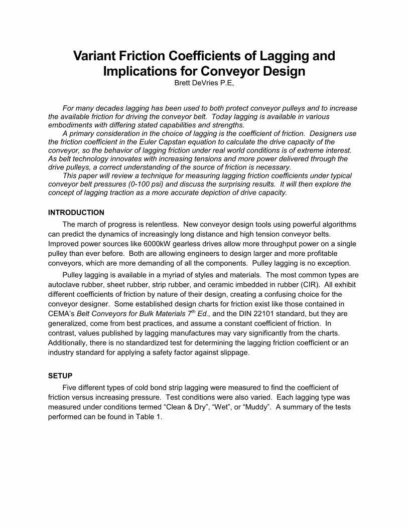
Some of the lagging
patterns were a makeup of
ceramic tiles and grooved
rubber features. The
ceramic tiles were 20mm
square with 1mm diameter
by 1 mm tall raised dimples.
The rubber compound was
a proprietary SBR/BR blend.
Pictures of the lagging types
are found in Table 2. The
full ceramic pattern has ceramic tiles comprising approximately 80% of the available contact
area with the belt and the remaining area as channels for the removal of water and solid
contaminates. The medium ceramic pattern has ceramic tiles covering 39% of the available
contact area and 34% as rubber. The diamond rubber ceramic pattern has ceramic tiles
covering 13% of the available contact area and 54% as rubber. The diamond rubber pattern
has rubber comprising 67% of the available contact area. The plain rubber pattern has rubber
comprising 80% of the available contact area.
Full ceramic Medium ceramic Diamond rubber
ceramic Diamond rubber Plain rubber
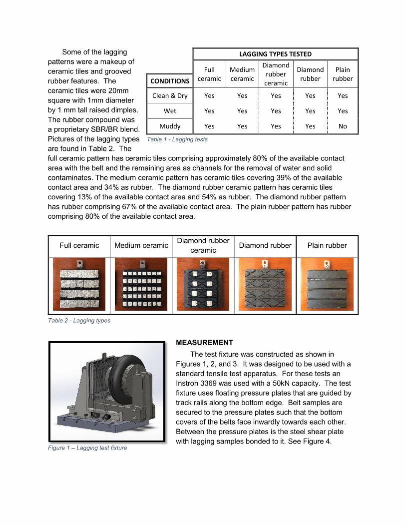
MEASUREMENT
The test fixture was constructed as shown in
Figures 1, 2, and 3. It was designed to be used with a
standard tensile test apparatus. For these tests an
Instron 3369 was used with a 50kN capacity. The test
fixture uses floating pressure plates that are guided by
track rails along the bottom edge. Belt samples are
secured to the pressure plates such that the bottom
covers of the belts face inwardly towards each other.
Between the pressure plates is the steel shear plate
with lagging samples bonded to it. See Figure 4.
LAGGING TYPES TESTED
Full ceramic
Medium ceramic
Diamond rubber ceramic
Diamond rubber
Plain rubber CONDITIONS
Clean & Dry Yes Yes Yes Yes Yes
Wet Yes Yes Yes Yes Yes
Muddy Yes Yes Yes Yes No
Figure 1 – Lagging test fixture
Table 1 - Lagging tests
Table 2 - Lagging types
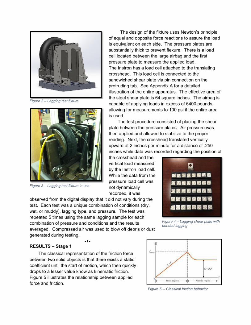
The design of the fixture uses Newton’s principle
of equal and opposite force reactions to assure the load
is equivalent on each side. The pressure plates are
substantially thick to prevent flexure. There is a load
cell located between the large airbag and the first
pressure plate to measure the applied load.
The Instron has a load cell attached to the translating
crosshead. This load cell is connected to the
sandwiched shear plate via pin connection on the
protruding tab. See Appendix A for a detailed
illustration of the entire apparatus. The effective area of
the steel shear plate is 64 square inches. The airbag is
capable of applying loads in excess of 6400 pounds,
allowing for measurements to 100 psi if the entire area
is used.
The test procedure consisted of placing the shear
plate between the pressure plates. Air pressure was
then applied and allowed to stabilize to the proper
reading. Next, the crosshead translated vertically
upward at 2 inches per minute for a distance of .250
inches while data was recorded regarding the position of
the crosshead and the
vertical load measured
by the Instron load cell.
While the data from the
pressure load cell was
not dynamically
recorded, it was
observed from the digital display that it did not vary during the
test. Each test was a unique combination of conditions (dry,
wet, or muddy), lagging type, and pressure. The test was
repeated 5 times using the same lagging sample for each
combination of pressure and conditions and the results
averaged. Compressed air was used to blow off debris or dust
generated during testing.
-+- RESULTS – Stage 1
The classical representation of the friction force
between two solid objects is that there exists a static
coefficient until the start of motion, which then quickly
drops to a lesser value know as kinematic friction.
Figure 5 illustrates the relationship between applied
force and friction.
Figure 2 – Lagging test fixture
Figure 4 – Lagging shear plate with bonded lagging
Figure 3 – Lagging test fixture in use
Figure 5 -- Classical friction behavior
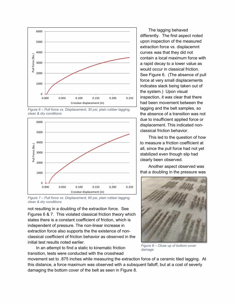
The lagging behaved
differently. The first aspect noted
upon inspection of the measured
extraction force vs. displacemnt
curves was that they did not
contain a local maximum force with
a rapid decay to a lower value as
would occur in classical friction.
See Figure 6. (The absence of pull
force at very small displacements
indicates slack being taken out of
the system.) Upon visual
inspection, it was clear that there
had been movement between the
lagging and the belt samples, so
the absence of a transition was not
due to insufficient applied force or
displacement. This indicated non-
classical friction behavior.
This led to the question of how
to measure a friction coefficient at
all, since the pull force had not yet
stabilized even though slip had
clearly been observed.
Another aspect observed was
that a doubling in the pressure was
not resulting in a doubling of the extraction force. See
Figures 6 & 7. This violated classical friction theory which
states there is a constant coefficient of friction, which is
independent of pressure. The non-linear increase in
extraction force also supports the the existence of non-
classical coefficient of friction behavior as observed in the
initial test results noted earlier.
In an attempt to find a static to kinematic friction
transition, tests were conducted with the crosshead
movement set to .875 inches while measuring the extraction force of a ceramic tiled lagging. At
this distance, a force maximum was observed with a subsquent falloff, but at a cost of severly
damaging the bottom cover of the belt as seen in Figure 8.
0
1000
2000
3000
4000
5000
6000
0.000 0.050 0.100 0.150 0.200 0.250
Pu
ll Fo
rce
(lb
s.)
Crossbar displacement (in)
0
1000
2000
3000
4000
5000
6000
0.000 0.050 0.100 0.150 0.200 0.250
Pu
ll Fo
rce
(lb
s.)
Crossbar displacement (in)
Figure 6 – Pull force vs. Displacement, 30 psi, plain rubber lagging, clean & dry conditions
Figure 8 – Close up of bottom cover damage
Figure 7 – Pull force vs. Displacement, 60 psi, plain rubber lagging, clean & dry conditions
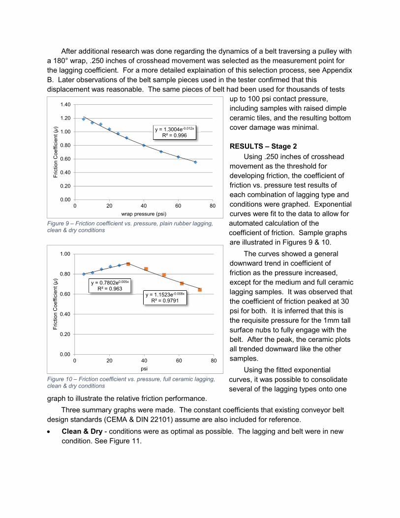
After additional research was done regarding the dynamics of a belt traversing a pulley with
a 180° wrap, .250 inches of crosshead movement was selected as the measurement point for
the lagging coefficient. For a more detailed explaination of this selection process, see Appendix
B. Later observations of the belt sample pieces used in the tester confirmed that this
displacement was reasonable. The same pieces of belt had been used for thousands of tests
up to 100 psi contact pressure,
including samples with raised dimple
ceramic tiles, and the resulting bottom
cover damage was minimal.
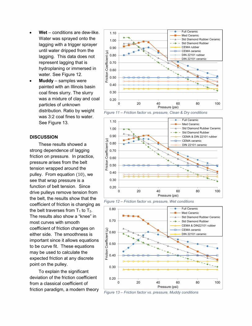
RESULTS – Stage 2
Using .250 inches of crosshead
movement as the threshold for
developing friction, the coefficient of
friction vs. pressure test results of
each combination of lagging type and
conditions were graphed. Exponential
curves were fit to the data to allow for
automated calculation of the
coefficient of friction. Sample graphs
are illustrated in Figures 9 & 10.
The curves showed a general
downward trend in coefficient of
friction as the pressure increased,
except for the medium and full ceramic
lagging samples. It was observed that
the coefficient of friction peaked at 30
psi for both. It is inferred that this is
the requisite pressure for the 1mm tall
surface nubs to fully engage with the
belt. After the peak, the ceramic plots
all trended downward like the other
samples.
Using the fitted exponential
curves, it was possible to consolidate
several of the lagging types onto one
graph to illustrate the relative friction performance.
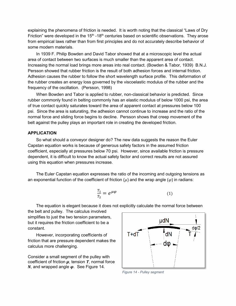
Three summary graphs were made. The constant coefficients that existing conveyor belt
design standards (CEMA & DIN 22101) assume are also included for reference.
Clean & Dry - conditions were as optimal as possible. The lagging and belt were in new
condition. See Figure 11.
y = 1.3004e-0.012x
R² = 0.996
0.00
0.20
0.40
0.60
0.80
1.00
1.20
1.40
0 20 40 60 80
Frictio
n C
oe
ffic
ien
t (µ
)
wrap pressure (psi)
y = 0.7802e0.005x
R² = 0.963y = 1.1523e-0.008x
R² = 0.9791
0.00
0.20
0.40
0.60
0.80
1.00
0 20 40 60 80
Frict
ion
Coe
ffic
ien
t (µ
)
psi
Figure 9 – Friction coefficient vs. pressure, plain rubber lagging, clean & dry conditions
Figure 10 – Friction coefficient vs. pressure, full ceramic lagging, clean & dry conditions
Wet – conditions are dew-like.
Water was sprayed onto the
lagging with a trigger sprayer
until water dripped from the
lagging. This data does not
represent lagging that is
hydroplaning or immersed in
water. See Figure 12.
Muddy – samples were
painted with an Illinois basin
coal fines slurry. The slurry
was a mixture of clay and coal
particles of unknown
distribution. Ratio by weight
was 3:2 coal fines to water.
See Figure 13.
DISCUSSION
These results showed a
strong dependence of lagging
friction on pressure. In practice,
pressure arises from the belt
tension wrapped around the
pulley. From equation (10), we
see that wrap pressure is a
function of belt tension. Since
drive pulleys remove tension from
the belt, the results show that the
coefficient of friction is changing as
the belt traverses from T1 to T2.
The results also show a “knee” in
most curves with smooth
coefficient of friction changes on
either side. The smoothness is
important since it allows equations
to be curve fit. These equations
may be used to calculate the
expected friction at any discrete
point on the pulley.
To explain the significant
deviation of the friction coefficient
from a classical coefficient of
friction paradigm, a modern theory
Figure 12 – Friction factor vs. pressure, Wet conditions
Figure 13 – Friction factor vs. pressure, Muddy conditions
Figure 11 – Friction factor vs. pressure, Clean & Dry conditions
0.20
0.30
0.40
0.50
0.60
0.70
0.80
0.90
1.00
1.10
0 20 40 60 80 100F
rictio
n C
oe
ffic
ien
t (µ
)Pressure (psi)
Full Ceramic
Med Ceramic
Std Diamond Rubber Ceramic
Std Diamond Rubber
CEMA rubber
CEMA ceramic
DIN 22101 rubber
DIN 22101 ceramic
0.20
0.30
0.40
0.50
0.60
0.70
0.80
0.90
1.00
1.10
0 20 40 60 80 100
Frict
ion
Coe
ffic
ien
t (µ
)
Pressure (psi)
Full Ceramic
Med Ceramic
Std Diamond Rubber Ceramic
Std Diamond Rubber
CEMA & DIN 22101 rubber
CEMA ceramic
DIN 22101 ceramic
0.20
0.30
0.40
0.50
0.60
0.70
0.80
0 20 40 60 80 100
Frict
ion
Coe
ffic
ien
t (µ
)
Pressure (psi)
Full Ceramic
Med Ceramic
Std Diamond Rubber Ceramic
Std Diamond Rubber
CEMA & DIN22101 rubber
CEMA ceramic
DIN 22101 ceramic
explaining the phenomena of friction is needed. It is worth noting that the classical “Laws of Dry
Friction” were developed in the 15th -18th centuries based on scientific observations. They arose
from empirical laws rather than from first principles and do not accurately describe behavior of
some modern materials.
In 1939 F. Philip Bowden and David Tabor showed that at a microscopic level the actual
area of contact between two surfaces is much smaller than the apparent area of contact.
Increasing the normal load brings more areas into real contact. (Bowden & Tabor, 1939) B.N.J.
Persson showed that rubber friction is the result of both adhesion forces and internal friction.
Adhesion causes the rubber to follow the short wavelength surface profile. This deformation of
the rubber creates an energy loss governed by the viscoelastic modulus of the rubber and the
frequency of the oscillation. (Persson, 1998)
When Bowden and Tabor is applied to rubber, non-classical behavior is predicted. Since
rubber commonly found in belting commonly has an elastic modulus of below 1000 psi, the area
of true contact quickly saturates toward the area of apparent contact at pressures below 100
psi. Since the area is saturating, the adhesion cannot continue to increase and the ratio of the
normal force and sliding force begins to decline. Persson shows that creep movement of the
belt against the pulley plays an important role in creating the developed friction.
APPLICATION
So what should a conveyor designer do? The new data suggests the reason the Euler
Capstan equation works is because of generous safety factors in the assumed friction
coefficient, especially at pressures below 70 psi. However, since available friction is pressure
dependent, it is difficult to know the actual safety factor and correct results are not assured
using this equation when pressures increase.
The Euler Capstan equation expresses the ratio of the incoming and outgoing tensions as
an exponential function of the coefficient of friction (µ) and the wrap angle (φ) in radians:
��
��= ��� (1)
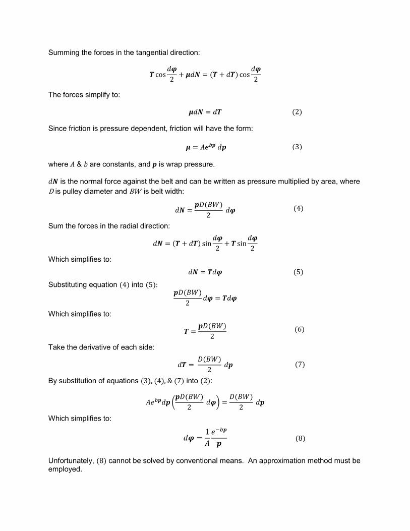
The equation is elegant because it does not explicitly calculate the normal force between
the belt and pulley. The calculus involved
simplifies to just the two tension parameters,
but it requires the friction coefficient to be a
constant.
However, incorporating coefficients of
friction that are pressure dependent makes the
calculus more challenging.
Consider a small segment of the pulley with coefficient of friction µ, tension T, normal force N, and wrapped angle �. See Figure 14. Figure 14 - Pulley segment
Summing the forces in the tangential direction:
� cos��
2+ ��� = (� + ��) cos
��
2
The forces simplify to:
��� = ��
Since friction is pressure dependent, friction will have the form:
� = ������
where A & b are constants, and p is wrap pressure. �� is the normal force against the belt and can be written as pressure multiplied by area, where
D is pulley diameter and BWis belt width:
�� =��(��)
2��
Sum the forces in the radial direction:
�� = (� + ��) sin��
2+ � sin
��
2
Which simplifies to:
�� = ���
Substituting equation (4) into (5):��(��)
2�� = ���
Which simplifies to:
� =��(��)
2
Take the derivative of each side:
�� = �(��)
2��
By substitution of equations (3),(4),&(7) into (2):
������ ���(��)
2��� =
�(��)
2��
Which simplifies to:
�� =1
�
����
�
Unfortunately, (8) cannot be solved by conventional means. An approximation method must be employed.
(5)
(6)
(7)
(8)
(2)
(4)
(3)
APPROXIMATION METHOD
Friction force is usually expressed
as coefficient of friction multiplied by a
normal force. Normal force is
distributed over the apparent area of
contact and could be expressed as a
pressure. So, pressure multiplied by
the coefficient of friction is the friction
force per unit area between the two
apparent areas, otherwise known as
shear stress. Conceptually, this could
be considered the grip or traction that
the lagging has on the belt.
The shear stress function (τ) at the surface interface between the lagging and the belt is:
�(�) = �������� ∗ �(�) (9) Wrap pressure due to tension (T)
between the belt and the pulley is given by Metlovic (Metlovic, 1996):
�������� = 2�
(��)�(10)
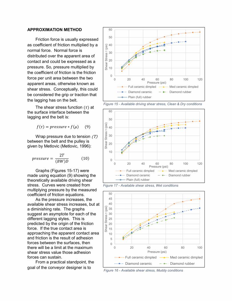
Graphs (Figures 15-17) were
made using equation (9) showing the theoretically available driving shear stress. Curves were created from multiplying pressure by the measured coefficient of friction equations.
As the pressure increases, the available shear stress increases, but at a diminishing rate. The graphs suggest an asymptote for each of the different lagging styles. This is predicted by the origin of the friction force. If the true contact area is approaching the apparent contact area and friction is the result of adhesion forces between the surfaces, then there will be a limit at the maximum shear stress value those adhesion forces can sustain.
From a practical standpoint, the
goal of the conveyor designer is to
0
10
20
30
40
50
60
0 20 40 60 80 100 120
Sh
ea
r S
tress τ
(psi)
Pressure (psi)
Full ceramic dimpled Med ceramic dimpled
Diamond ceramic Diamond rubber
Plain (full) rubber
Figure 15 - Available driving shear stress, Clean & Dry conditions
0
10
20
30
40
50
60
0 20 40 60 80 100 120
Sh
ea
r S
tress
τ (
psi)
Pressure (psi)
Full ceramic dimpled Med ceramic dimpled
Diamond ceramic Diamond rubber
Plain (full) rubber
0
5
10
15
20
25
30
35
40
45
50
0 20 40 60 80 100
Sh
ea
r S
tress
τ (p
si)
Pressure (psi)
Full ceramic dimpled Med ceramic dimpled
Diamond ceramic Diamond rubber
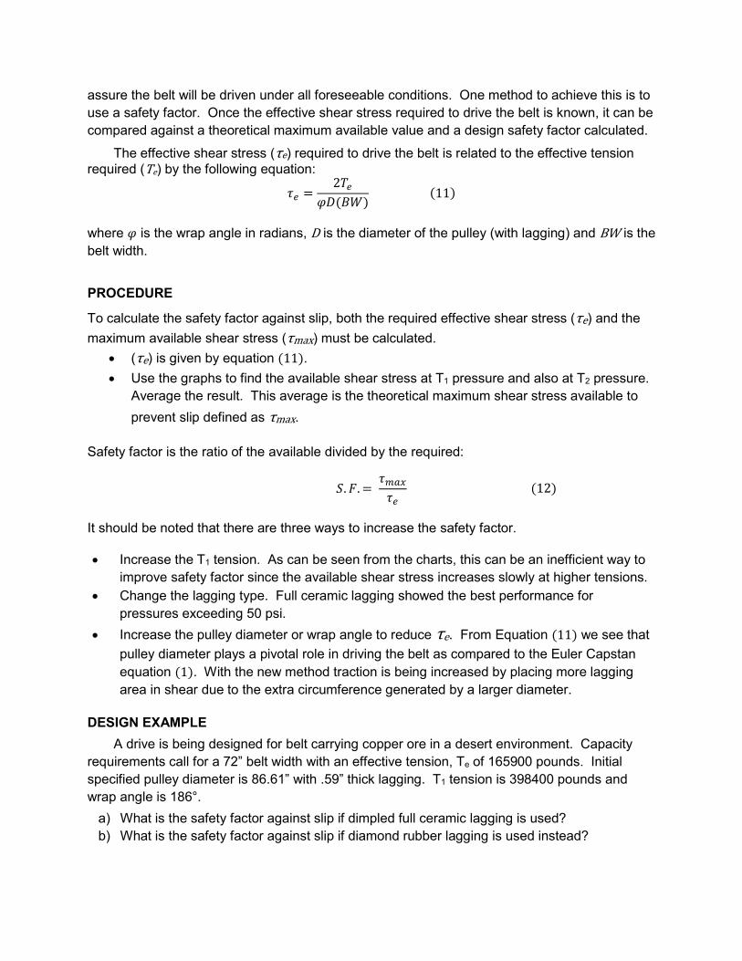
Figure 17 - Available shear stress, Wet conditions
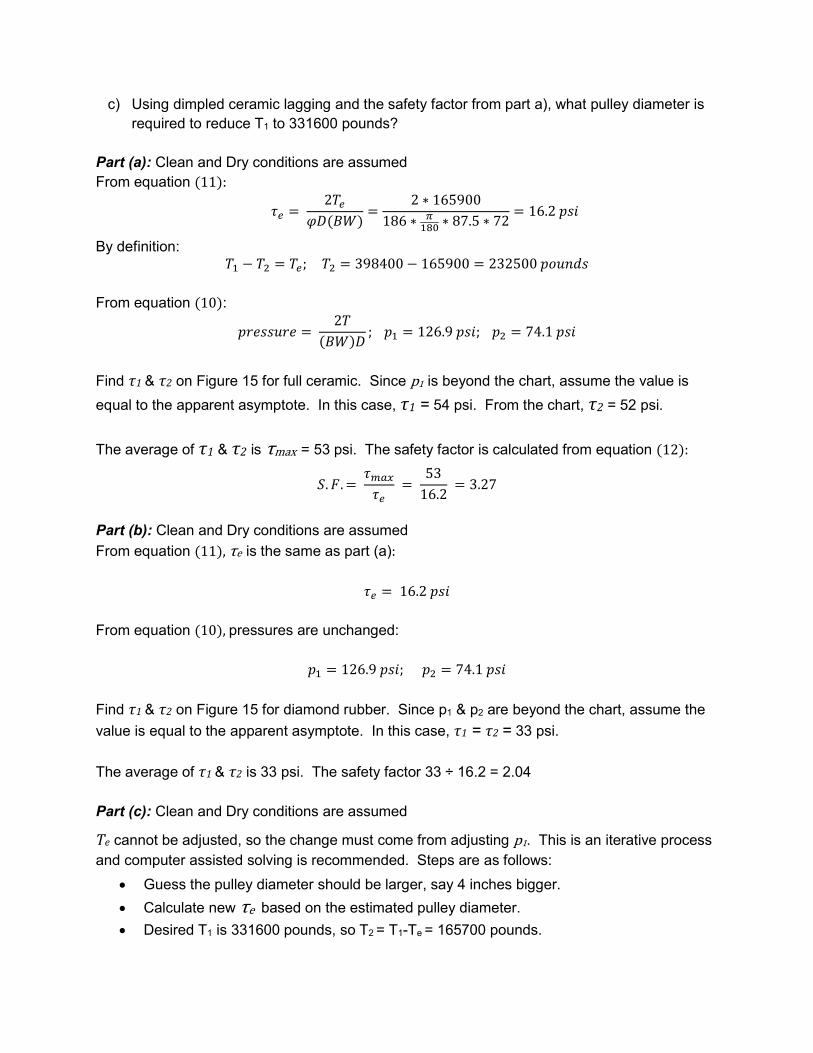
Figure 16 - Available shear stress, Muddy conditions
assure the belt will be driven under all foreseeable conditions. One method to achieve this is to
use a safety factor. Once the effective shear stress required to drive the belt is known, it can be
compared against a theoretical maximum available value and a design safety factor calculated.
The effective shear stress (τe) required to drive the belt is related to the effective tension required (Te) by the following equation:
�� =2��
��(��)(11)
where � is the wrap angle in radians, D is the diameter of the pulley (with lagging) and BW is the
belt width.
PROCEDURE
To calculate the safety factor against slip, both the required effective shear stress (τe) and the
maximum available shear stress (τmax) must be calculated.
(τe) is given by equation (11).
Use the graphs to find the available shear stress at T1 pressure and also at T2 pressure.
Average the result. This average is the theoretical maximum shear stress available to
prevent slip defined as τmax.
Safety factor is the ratio of the available divided by the required:
�. �. = ����
��
It should be noted that there are three ways to increase the safety factor.
Increase the T1 tension. As can be seen from the charts, this can be an inefficient way to
improve safety factor since the available shear stress increases slowly at higher tensions.
Change the lagging type. Full ceramic lagging showed the best performance for
pressures exceeding 50 psi.
Increase the pulley diameter or wrap angle to reduce τe. From Equation (11) we see that
pulley diameter plays a pivotal role in driving the belt as compared to the Euler Capstan
equation (1). With the new method traction is being increased by placing more lagging
area in shear due to the extra circumference generated by a larger diameter.
DESIGN EXAMPLE
A drive is being designed for belt carrying copper ore in a desert environment. Capacity
requirements call for a 72” belt width with an effective tension, Te of 165900 pounds. Initial
specified pulley diameter is 86.61” with .59” thick lagging. T1 tension is 398400 pounds and
wrap angle is 186°.
a) What is the safety factor against slip if dimpled full ceramic lagging is used?
b) What is the safety factor against slip if diamond rubber lagging is used instead?
(12)
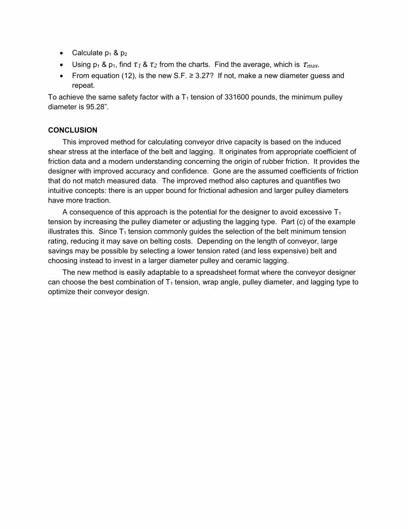
c) Using dimpled ceramic lagging and the safety factor from part a), what pulley diameter is
required to reduce T1 to 331600 pounds?
Part (a): Clean and Dry conditions are assumed
From equation (11):
�� = 2��
��(��)=
2 ∗ 165900
186 ∗ ����
∗ 87.5 ∗ 72= 16.2���
By definition: �� − �� = ��;�� = 398400 − 165900 = 232500������
From equation (10):
�������� = 2�
(��)�;�� = 126.9���;�� = 74.1���
Find τ1 & τ2 on Figure 15 for full ceramic. Since p1 is beyond the chart, assume the value is
equal to the apparent asymptote. In this case, τ1 = 54 psi. From the chart, τ2 = 52 psi.
The average of τ1 & τ2 is τmax = 53 psi. The safety factor is calculated from equation (12):
�. �. = ����
�� =
53
16.2 = 3.27
Part (b): Clean and Dry conditions are assumed
From equation (11),τe is the same as part (a):
�� = 16.2���
From equation (10),pressures are unchanged:
�� = 126.9���; �� = 74.1���
Find τ1 & τ2 on Figure 15 for diamond rubber. Since p1 & p2 are beyond the chart, assume the
value is equal to the apparent asymptote. In this case, τ1 = τ2 = 33 psi.
The average of τ1 & τ2 is 33 psi. The safety factor 33 ÷ 16.2 = 2.04
Part (c): Clean and Dry conditions are assumed
Te cannot be adjusted, so the change must come from adjusting p1. This is an iterative process
and computer assisted solving is recommended. Steps are as follows:
Guess the pulley diameter should be larger, say 4 inches bigger.
Calculate new τe based on the estimated pulley diameter.
Desired T1 is 331600 pounds, so T2 = T1-Te = 165700 pounds.
Calculate p1 & p2
Using p1 & p1, find τ1 & τ2 from the charts. Find the average, which is τmax.
From equation (12), is the new S.F. ≥ 3.27? If not, make a new diameter guess and
repeat.
To achieve the same safety factor with a T1 tension of 331600 pounds, the minimum pulley
diameter is 95.28”.
CONCLUSION
This improved method for calculating conveyor drive capacity is based on the induced
shear stress at the interface of the belt and lagging. It originates from appropriate coefficient of
friction data and a modern understanding concerning the origin of rubber friction. It provides the
designer with improved accuracy and confidence. Gone are the assumed coefficients of friction
that do not match measured data. The improved method also captures and quantifies two
intuitive concepts: there is an upper bound for frictional adhesion and larger pulley diameters
have more traction.
A consequence of this approach is the potential for the designer to avoid excessive T1
tension by increasing the pulley diameter or adjusting the lagging type. Part (c) of the example
illustrates this. Since T1 tension commonly guides the selection of the belt minimum tension
rating, reducing it may save on belting costs. Depending on the length of conveyor, large
savings may be possible by selecting a lower tension rated (and less expensive) belt and
choosing instead to invest in a larger diameter pulley and ceramic lagging.
The new method is easily adaptable to a spreadsheet format where the conveyor designer
can choose the best combination of T1 tension, wrap angle, pulley diameter, and lagging type to
optimize their conveyor design.
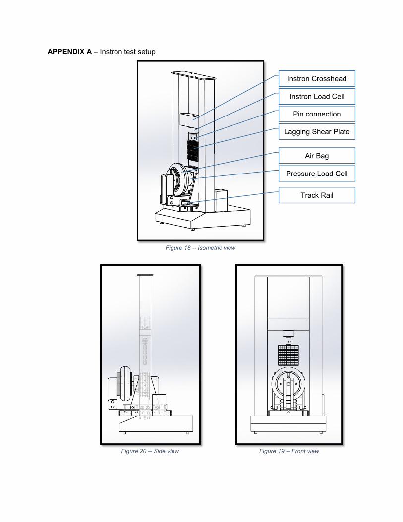
APPENDIX A – Instron test setup
Lagging Shear Plate
Instron Load Cell
Instron Crosshead
Pin connection
Pressure Load Cell
Air Bag
Figure 20 -- Side view Figure 19 -- Front view
Figure 18 -- Isometric view
Track Rail
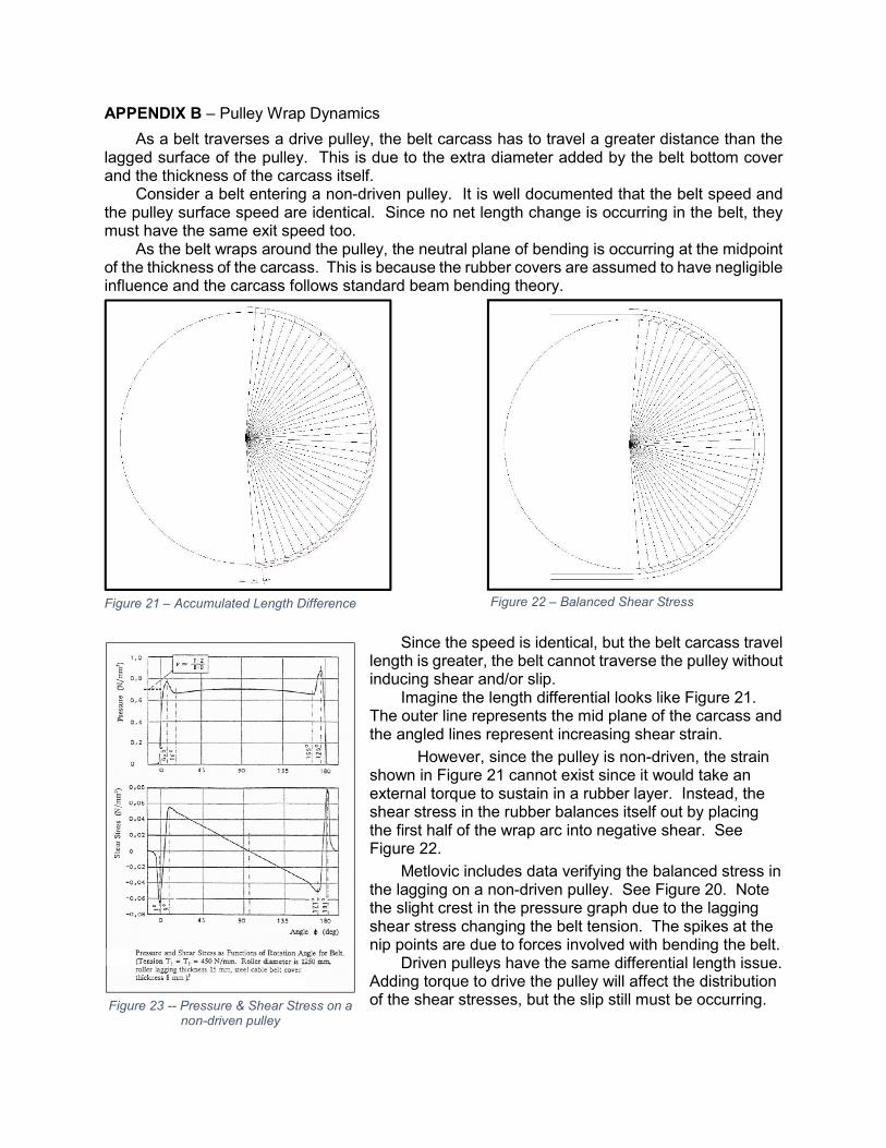
APPENDIX B – Pulley Wrap Dynamics
As a belt traverses a drive pulley, the belt carcass has to travel a greater distance than the lagged surface of the pulley. This is due to the extra diameter added by the belt bottom cover and the thickness of the carcass itself.
Consider a belt entering a non-driven pulley. It is well documented that the belt speed and the pulley surface speed are identical. Since no net length change is occurring in the belt, they must have the same exit speed too.
As the belt wraps around the pulley, the neutral plane of bending is occurring at the midpoint of the thickness of the carcass. This is because the rubber covers are assumed to have negligible influence and the carcass follows standard beam bending theory.
Since the speed is identical, but the belt carcass travel
length is greater, the belt cannot traverse the pulley without inducing shear and/or slip.
Imagine the length differential looks like Figure 21. The outer line represents the mid plane of the carcass and the angled lines represent increasing shear strain.
However, since the pulley is non-driven, the strain shown in Figure 21 cannot exist since it would take an external torque to sustain in a rubber layer. Instead, the shear stress in the rubber balances itself out by placing the first half of the wrap arc into negative shear. See Figure 22.
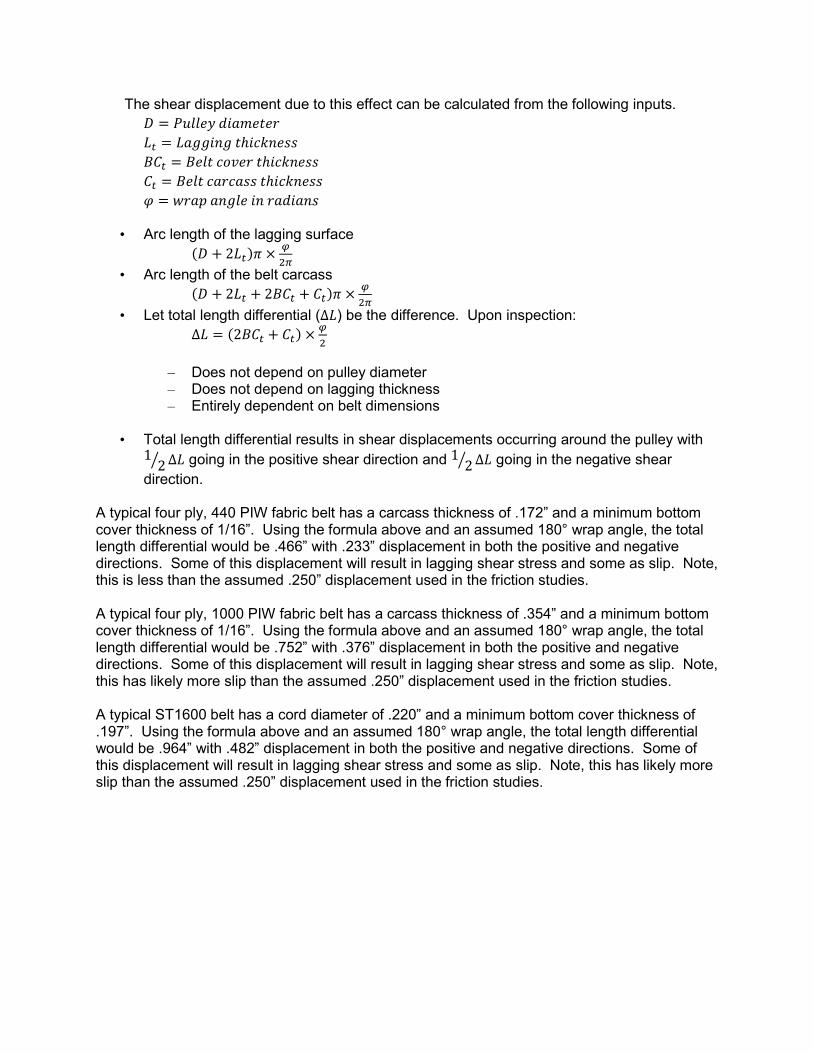
Metlovic includes data verifying the balanced stress in the lagging on a non-driven pulley. See Figure 20. Note the slight crest in the pressure graph due to the lagging shear stress changing the belt tension. The spikes at the nip points are due to forces involved with bending the belt.
Driven pulleys have the same differential length issue. Adding torque to drive the pulley will affect the distribution of the shear stresses, but the slip still must be occurring.
Figure 21 – Accumulated Length Difference Figure 22 – Balanced Shear Stress
Figure 23 -- Pressure & Shear Stress on a non-driven pulley
The shear displacement due to this effect can be calculated from the following inputs.
� = ��������������
�� = ��������ℎ�������
��� = ����������ℎ�������
�� = ������������ℎ�������
� = ������������������
• Arc length of the lagging surface
(� + 2��)� �
��
• Arc length of the belt carcass
(� + 2�� + 2��� + ��)� �
��
• Let total length differential (∆�) be the difference. Upon inspection:
∆� = (2��� + ��) ×�
�
– Does not depend on pulley diameter – Does not depend on lagging thickness – Entirely dependent on belt dimensions
• Total length differential results in shear displacements occurring around the pulley with
12� ∆� going in the positive shear direction and 1 2� ∆� going in the negative shear
direction.
A typical four ply, 440 PIW fabric belt has a carcass thickness of .172” and a minimum bottom cover thickness of 1/16”. Using the formula above and an assumed 180° wrap angle, the total length differential would be .466” with .233” displacement in both the positive and negative directions. Some of this displacement will result in lagging shear stress and some as slip. Note, this is less than the assumed .250” displacement used in the friction studies. A typical four ply, 1000 PIW fabric belt has a carcass thickness of .354” and a minimum bottom cover thickness of 1/16”. Using the formula above and an assumed 180° wrap angle, the total length differential would be .752” with .376” displacement in both the positive and negative directions. Some of this displacement will result in lagging shear stress and some as slip. Note, this has likely more slip than the assumed .250” displacement used in the friction studies. A typical ST1600 belt has a cord diameter of .220” and a minimum bottom cover thickness of .197”. Using the formula above and an assumed 180° wrap angle, the total length differential would be .964” with .482” displacement in both the positive and negative directions. Some of this displacement will result in lagging shear stress and some as slip. Note, this has likely more slip than the assumed .250” displacement used in the friction studies.
REFERENCES Bowden, F., & Tabor, D. (1939). The area of contact between stationary and between moving
surfaces. Proc. R. Soc. A, 169, 391-413. Metlovic, P. M. (1996). Mechanics of Rubber Covered Conveyor Rollers. Akron, OH: Ph.D.
Dissertation: The University of Akron. Persson, B. (1998). On the theory of rubber friction. Surface Science, 401, 445-454.
Variant Friction Coefficients of Lagging and Implications for Conveyor Design
Brett DeVries P.E.
Flexible Steel Lacing Company, USA
Synopsis
Modern conveyor design is creating demand for extremely large and expensive belts with greater tensions and power capabilities than ever before. These belts are driven by lagged pulleys, and it would be valuable to prove this lagging will perform under the increased tension and drive requirements.
A test apparatus is described for measuring lagging friction, and friction coefficients are measured under uniform pressurized loading using a tensile test machine. Applied pressures range from 5 to 100 psi, including some measurements to 120 psi for various lagging types. The result is a strong dependence between the coefficient of friction and pressure. This is contrary to the industry practice of assuming a constant friction factor and utilizing the Euler Capstan equation to calculate allowable tension ratios around the drive pulley. An attempt is made to modify the Euler Capstan equation to incorporate pressure dependent friction, but is shown to be unsolvable. As a result, an approximation method based on the generated shear stress, or traction, at the lagging surface is presented.
The data presented suggests the existence of a maximum available traction, regardless of increasing pressure, for each lagging design. Using the approximation method, it is shown that belt tension, lagging type, wrap angle, and pulley diameter are all factors affecting drive capacity. It is also shown that changes in the pulley diameter, wrap angle, or lagging type can have a strong influence on the minimum tension rating required for the conveyor belt.
Recommended