Deme, demography, vital statistics of
populations
Population parameters, mean and variance
“Life” Tables: Cohort vs. Segment Samples
Age and sex specificity
Homocide example: Chicago vs. England
Numbers dying in each age interval
Discrete vs. continuous approaches
Force of Mortality qx
Age-specific survivorship lx
Type I, II, III survivorship
(rectangular, diagonal, inverse hyperbolic)

Expectation of further life,
Age-specific fecundity, mx
Age of first reproduction, alpha, —
menarche
Age of last reproduction, omega,
Realized fecundity at age x, lxmx
Net Reproductive rate
Human body louse, R0 = 31
Generation Time, T = xlxmx
Reproductive value, vx
Stable vs. changing populations
Residual reproductive value

Age of first reproduction, alpha, —
menarche
Age of last reproduction, omega,
Reproductive value vx , Expectation of
future offspring
Stable vs. changing populations
Present value of all expected future
progeny
Residual reproductive value
Intrinsic rate of increase (little r, per capita = b - d)
J-shaped exponential runaway population growth
Differential equation: dN/dt = rN = (b - d)N, Nt = N0 ert
Demographic and Environmental Stochasticity

T, Generation time = average time from one gener- ation to the next (average time from egg to egg)
vx = Reproductive Value = Age-specific expectation
of all future offspring
p.143, right hand equation“dx” should be “dt”

In populations that are expanding or contracting, reproductive value is more complicated. Must weight progeny produced earlier as being worth more in expanding populations, but worth less in declining populations. The verbal definition is also changed to “the present value of all future offspring”
p.146, left handequation left oute-rt term
QuickTime™ and a decompressor
are needed to see this picture.

vx = mx + (lt / lx ) mt
Residual reproductive value =
age-specific expectation of
offspring in distant future
vx* = (lx+1 / lx ) vx+1

Intrinsic rate of increase (per
capita, instantaneous)
r = b - d
rmax and ractual — lx varies inversely
with mx
Stable (stationary) age distributions
Leslie Matrices (Projection Matrix)
Dominant Eigenvalue = Finite rate of
increase

Illustration of Calculation of Ex, T, R0, and vx in a Stable Population with Discrete Age Classes_____________________________________________________________________
Age Expectation Reproductive Weighted of Life Value
Survivor- Realized by Realized Ex vx
Age (x) ship Fecundity Fecundity Fecundity lx mx lxmx x lxmx
_____________________________________________________________________0 1.0 0.0 0.00 0.00 3.40 1.001 0.8 0.2 0.16 0.16 3.00 1.252 0.6 0.3 0.18 0.36 2.67 1.403 0.4 1.0 0.40 1.20 2.50 1.654 0.4 0.6 0.24 0.96 1.50 0.655 0.2 0.1 0.02 0.10 1.00 0.106 0.0 0.0 0.00 0.00 0.00 0.00Sums 2.2 (GRR) 1.00 (R0) 2.78 (T) _____________________________________________________________________E0 = (l0 + l1 + l2 + l3 + l4 + l5)/l0 = (1.0 + 0.8 + 0.6 + 0.4 + 0.4 + 0.2) / 1.0 = 3.4 / 1.0E1 = (l1 + l2 + l3 + l4 + l5)/l1 = (0.8 + 0.6 + 0.4 + 0.4 + 0.2) / 0.8 = 2.4 / 0.8 = 3.0E2 = (l2 + l3 + l4 + l5)/l2 = (0.6 + 0.4 + 0.4 + 0.2) / 0.6 = 1.6 / 0.6 = 2.67E3 = (l3 + l4 + l5)/l3 = (error: extra terms) 0.4 + 0.4 + 0.2) /0.4 = 1.0 / 0.4 = 2.5E4 = (l4 + l5)/l4 = (error: extra terms) 0.4 + 0.2) /0.4 = 0.6 / 0.4 = 1.5E5 = (l5) /l5 = 0.2 /0.2 = 1.0v1 = (l1/l1)m1+(l2/l1)m2+(l3/l1)m3+(l4/l1)m4+(l5/l1)m5 = 0.2+0.225+0.50+0.3+0.025 = 1.25 v2 = (l2/l2)m2 + (l3/l2)m3 + (l4/l2)m4 + (l5/l2)m5 = 0.30+0.67+0.40+ 0.03 = 1.40 v3 = (l3/l3)m3 + (l4/l3)m4 + (l5/l3)m5 = 1.0 + 0.6 + 0.05 = 1.65 v4 = (l4/l4)m4 + (l5/l4)m5 = 0.60 + 0.05 = 0.65v5 = (l5/l5)m5 = 0.1
___________________________________________________________________________
p. 144 deleteextra terms (red)

QuickTime™ and a decompressor
are needed to see this picture.
QuickTime™ and a decompressor
are needed to see this picture.
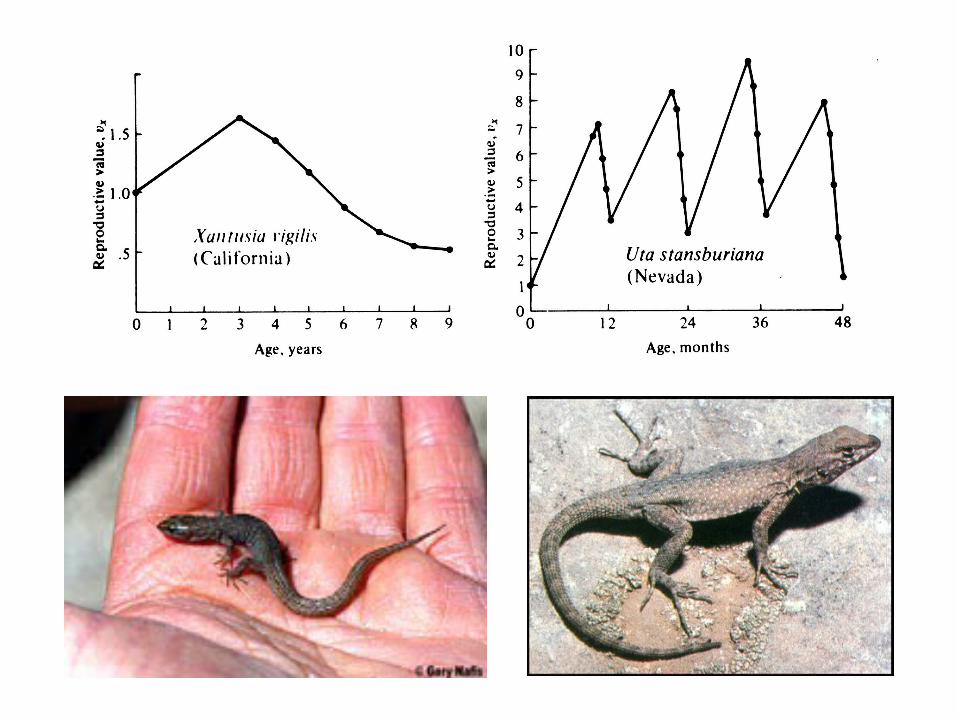
Stable age distribution
Stationary age distribution


Leslie Matrix (a projection matrix)
Assume lx and mx values are fixed and independent ofpopulation size. px = lx+1 /lx Mortality precedes reproduction.


Leslie Matrix (a projection matrix)
Assume lx and mx values are fixed and independent ofpopulation size. px = lx+1 /lx Mortality precedes reproduction.

n (t +1) = L n(t )
n (t +2) = L n(t +1)
= L [Ln(t)] = L2 n(t )
n (t +k) = Lk n(t )
With a fixed Leslie matrix, any age
distribution converges on the stable age
distribution in a few generations. When
this distribution is reached, each age
class changes at the same rate and n(t
+1) = n(t). is the finite rate of increase, the real part of the dominant
root or the eigenvalue of the Leslie
matrix (an amplification factor). See
Handout No. 1.

Reproductive value, intrinsic rate of increase (little r, per capita)
J-shaped exponential runaway population growth
Differential equation: dN/dt = rN = (b - d)N, Nt = N0 ert
Demographic and Environmental Stochasticity
Evolution of Reproductive Tactics: semelparous versus iteroparous
Reproductive effort (parental investment)

Estimated Maximal Instantaneous Rates of Increase (rmax, Per Capita Per Day) and Mean Generation Times ( in Days) for a Variety of Organisms____________________________________________________________________________Taxon Species rmax Generation Time (T)------------------------------------------------------------------------------------------------------------------Bacterium Escherichia coli ca. 60.0 0.014Protozoa Paramecium aurelia 1.24 0.33–0.50Protozoa Paramecium caudatum 0.94 0.10–0.50Insect Tribolium confusum 0.120 ca. 80 Insect Calandra oryzae 0.110(.08–.11) 58Insect Rhizopertha dominica 0.085(.07–.10) ca. 100Insect Ptinus tectus 0.057 102Insect Gibbum psylloides 0.034 129Insect Trigonogenius globulosus 0.032 119Insect Stethomezium squamosum 0.025 147Insect Mezium affine 0.022 183Insect Ptinus fur 0.014 179Insect Eurostus hilleri 0.010 110Insect Ptinus sexpunctatus 0.006 215Insect Niptus hololeucus 0.006 154Mammal Rattus norwegicus 0.015 150Mammal Microtus aggrestis 0.013 171Mammal Canis domesticus 0.009 ca. 1000Insect Magicicada septendcim 0.001 6050Mammal Homo sapiens 0.0003 ca. 7000
_____________________________________________________

Exponential population growth under the assumption that the rate of increase per individual, r, remains constant with changes in population density. Note that a straight-line estimate of the rate of population growth at time t becomes more and more accurate as t1 and t2 converge; in the limit, as t1 and t2 approach t, or ∆t —> 0, the rate of population growth equals the slope of a line tangent to the curve at time t (open circle).
J - shaped exponential population growth
http://www.zo.utexas.edu/courses/THOC/exponential.growth.html

Instantaneous rate of change of N
at time t is total births minus
total deaths
dN/dt = bN – dN = (b – d )N = rN
Nt = N0 ert
log Nt = log N0 + log ert = log N0
+ rt
log R0 = log 1 + rt r = log
R0 / T
r = log or = er
~

Demographic and Environmental
Stochasticity
random walks, especially important in
small populations
Evolution of Reproductive Tactics
Semelparous versus Interoparous
Big Bang versus Repeated Reproduction
Reproductive Effort (parental
investment)
Age of First Reproduction, alpha,
Age of Last Reproduction, omega,

Mola mola
(“Ocean Sunfish”)
200 million eggs!
Poppy (Papaver rhoeas)produces only 4 seeds when stressed, but as many as 330,000 under ideal conditions


How much should an organism invest in any given act of reproduction? R. A. Fisher (1930) anticipated this question long ago:
“It would be instructive to know not only by what physiological mechanism a just apportionment is made between the nutriment devoted to the gonads and that devoted to the rest of the parental organism, but also what circumstances in the life history and environment would render profitable the diversion of a greater or lesser share of available resources towards reproduction.” [Italics added for emphasis.]
Reproductive Effort
R. A. Fisher
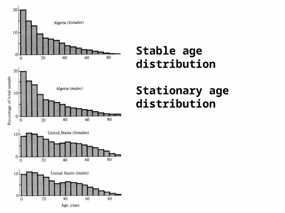
Joint Evolution of Rates of Reproduction and Mortality
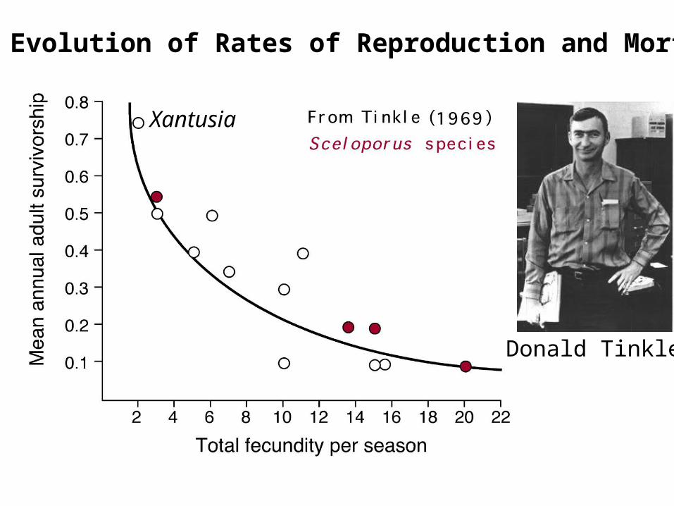
Donald Tinkle
Xantusia


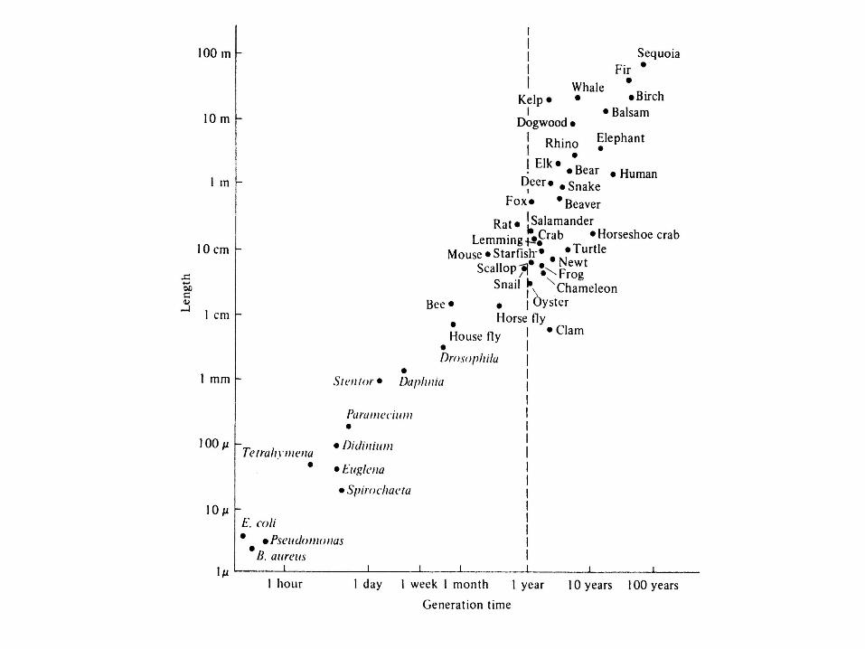
Inverserelationshipbetween rmax
and generation time, T

Asplanchna (Rotifer)
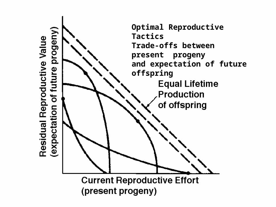
Optimal Reproductive TacticsTrade-offs between present progenyand expectation of future offspring
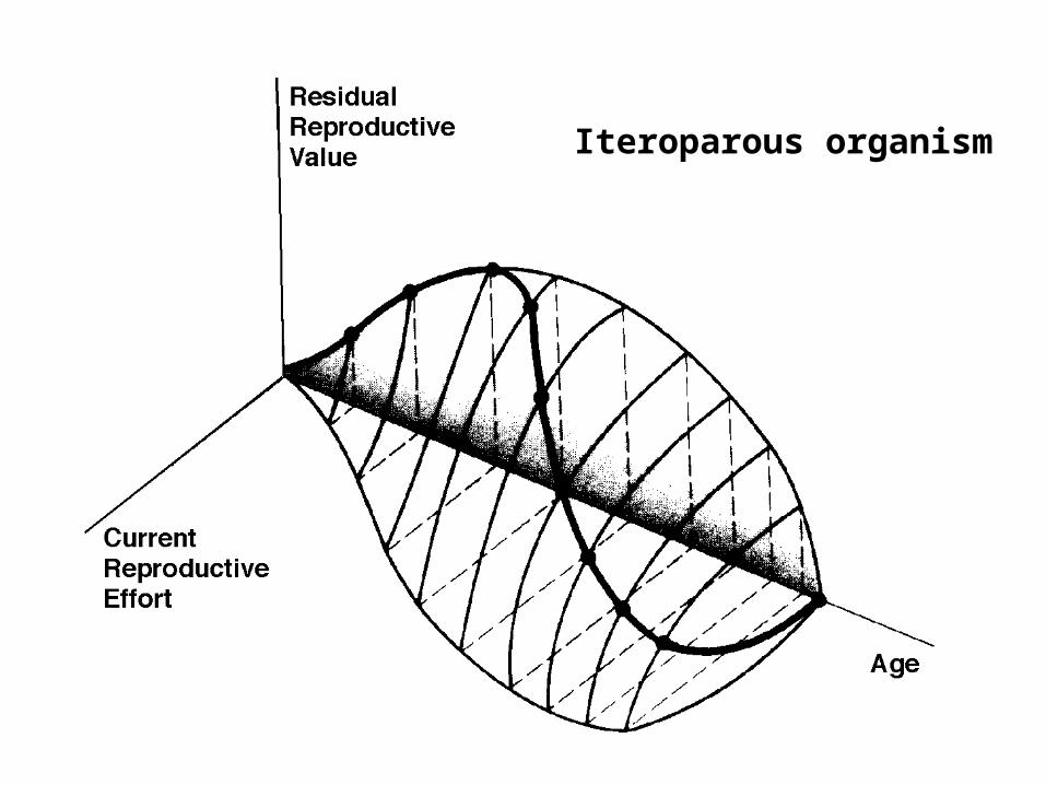
Iteroparous organism
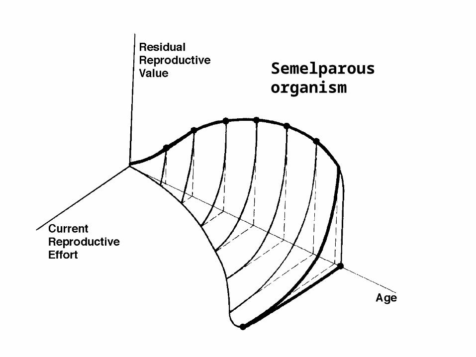
Semelparous organism
Recommended