User’s Manual of the Intercalibration Spreadsheets Sebastian Birk, Nigel Willby and Dirk Nemitz
January 2011
User’s Manual of the Intercalibration Spreadsheets v3
Table of Contents
1 Introduction ..................................................................................................................................... 3 2 Spreadsheet selection .................................................................................................................... 4 3 IC Option 2 spreadsheets ............................................................................................................... 5
3.1 Input requirements ................................................................................................................................. 5 3.1.1 Sheet “Bm” ............................................................................................................................................. 5 3.1.2 Sheet “data” ........................................................................................................................................... 5
3.2 Steps of calculation ................................................................................................................................ 5 3.2.1 Linear regression ................................................................................................................................... 5 3.2.2 Benchmark standardisation .................................................................................................................... 5 3.2.3 Boundary translation .............................................................................................................................. 6 3.2.4 Boundary bias ........................................................................................................................................ 6 3.2.5 Boundary harmonisation ........................................................................................................................ 7
4 IC Option 3 spreadsheets ............................................................................................................... 9 4.1 Input requirements ................................................................................................................................. 9
4.1.1 Sheet “Bm” ............................................................................................................................................. 9 4.1.2 Sheet “data” ........................................................................................................................................... 9
4.2 Steps of calculation ................................................................................................................................ 9 4.2.1 Linear regression against pseudo-common metric ................................................................................. 9 4.2.2 Benchmark standardisation .................................................................................................................. 10 4.2.3 Boundary translation ............................................................................................................................ 12 4.2.4 Boundary bias ...................................................................................................................................... 12 4.2.5 Boundary harmonisation ...................................................................................................................... 13 4.2.6 Class agreement .................................................................................................................................. 14
5 References .................................................................................................................................... 16

User’s Manual of the Intercalibration Spreadsheets
3
1 Introduction
This document explains the use and functions of the four intercalibration spreadsheet files
that can be downloaded from http://www.uni-due.de/hydrobiology/publications/birk.shtml,
section “Intercalibration tools”1:
IC_Opt2_div.xlsx
IC_Opt2_sub.xlsx
IC_Opt3_div.xlsx
IC_Opt3_sub.xlsx
The files are designed to support the analytical process of comparing and harmonising the
good status boundaries of national assessment methods according to Annex V of CIS
(2010).
The spreadsheets are programmed in MS Excel 2007 (.xlsx) and are capable to process up
to 16 national assessment methods and 4,000 sample data entries. Cells for data entry are
marked in yellow; all other cells are protected from modification2.
In the following section we describe how to select the spreadsheet version required for your
exercise. Specifications on IC Option 2 and 3 spreadsheets form the main part of the
document. We suggest to directly refer to the relevant section of this manual after you have
identified the appropriate spreadsheet version. Note that the Annex V criterion of "class
agreement" can only be calculated by the Option 3 spreadsheets.
We welcome the use of the spreadsheets for facilitating your intercalibration
exercise. However, we strongly advise you to perform independent calculations
of boundary comparison and harmonisation. The spreadsheets are primarily
designed to quickly check the implications of boundary adjustment, and as a
means to review your outcomes.
1 This manual and cited references can also be downloaded here.
2 The spreadsheets are not blank but contain artificial datasets used to test the files. To run your own analysis you
need to overwrite these data.
User’s Manual of the Intercalibration Spreadsheets
4
2 Spreadsheet selection
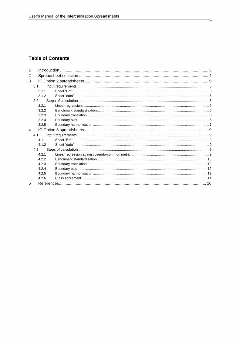
Four different spreadsheet versions were designed to allow for various alternatives of
boundary comparison in intercalibration. Select the appropriate version by (1) choosing the
IC Option followed in your intercalibration exercise (see CIS, 2010), and (2) identifying the
relationships of anthropogenic pressure against national assessment results (i.e. EQRs)
(Figure 1).
Figure 1: Types of pressure-impact-relationships and options of calculating the benchmark standardisation
Upper diagram: Standardisation is done by division if differences in the biological assessment results (ICM) between
national methods (green and red crosses) vanish with increasing pressure.
Lower diagram: Standardisation is done by subtraction if differences remain throughout the entire pressure gradient.
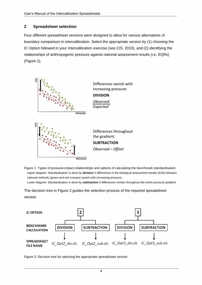
The decision tree in Figure 2 guides the selection process of the required spreadsheet
version.
Figure 2: Decision tree for selecting the appropriate spreadsheet version
Differences throughoutthe gradient:
SUBTRACTION
Observed – Offset
Differences vanish withincreasing pressure:
DIVISION
ObservedExpected
User’s Manual of the Intercalibration Spreadsheets
5
3 IC Option 2 spreadsheets
3.1 Input requirements
3.1.1 Sheet “Bm”
The reference values (usually “1.00”) and all national class boundaries (as EQR values)
need to be specified for each method participating in the intercalibration exercise. Select an
appropriate identifier for the national methods as table headers, and use the same identifier
also in the Sheet data.
3.1.2 Sheet “data”
In IC Option 2 the intercalibration analyses are carried out on the basis of separate datasets
related to each national method. The spreadsheet on IC Option 2 requires information about:
Sample code
National method (same as in Sheet Bm)
National EQR
Common metric
Furthermore, benchmark sites have to be selected for each method (see Birk & Willby 2010).
All data are entered one below the other in Sheet data for the individual methods.
Note: Never delete entire rows or columns in the data input sheets.
3.2 Steps of calculation
3.2.1 Linear regression
The Option 2 spreadsheet establishes ordinary least-square regressions for each national
dataset. Sheets tdata and gdata are used to arrange the data for the subsequent analyses.
On this basis the regression the graphs in Sheet reg are plotted. These graphs include
sample plots, regression formulae and R2 values. Note that no benchmark standardisation
has been applied to the data presented in this sheet.
Sheet calc specifies details of the regressions (rows 2-6). Here, it is possible to manually
enter regression slopes for testing the effects of different slope values on the intercalibration
outcomes3.
3.2.2 Benchmark standardisation
Row(s) 8(-10) of Sheet calc include the details for the benchmark standardisation. The
“Median ICM” is defined as the median of the common metric values at benchmark sites
3 This may be useful in cases of weak regressions (e.g. low number of samples, low R
2 values).

User’s Manual of the Intercalibration Spreadsheets
6
(specified by the user in Sheet data)4. This median is calculated separately for each national
method/dataset.
Benchmark calculation: Division5
Standardisation by division is done by dividing the EQR values belonging to a national
method by the median value of benchmark sites of this country.
Benchmark calculation: Subtraction6
The “Offset” of method x [Offx] is the deviation of the national median [nMedx] to the average
of all benchmark medians [ØMed] in common metric units, i.e.
Offx = ØMed – nMedx
For benchmark standardisation this number is added to the national reference and boundary
values before boundary comparison (see rows 18-22). The spreadsheet also allows for a
manual input of offsets. This may be useful to test the effects of differing benchmarks on the
intercalibration outcomes.
3.2.3 Boundary translation
Rows 16-20 (version: division) or 18-22 (version: subtraction) of Sheet calc present the
position of the national reference7 and boundary values (1) after translation into common
metric scale by linear regressions, and (2) after benchmark standardisation. For your
convenience the original values you entered into Sheet Bm are listed in rows 10-14 (div) or
12-16 (sub).
3.2.4 Boundary bias
Boundary bias is one of the two components to check the comparability of national quality
classifications (CIS, 2010). Boundary bias is defined as the deviation of the relevant national
class boundary (high-good or good-moderate) from the average boundary position derived
from all methods participating in the exercise (“harmonisation guideline”). Boundary bias is
expressed in national class equivalents and must not exceed 0.25 units. All elements
required to calculate boundary bias are shown in Figure 3.
4 Note that the total number of benchmark sites is specified in Sheet adj (row 26).
5 Relevant for spreadsheet file IC_opt2_div.xls
6 Relevant for spreadsheet file IC_opt2_sub.xls
7 For the translation of the national reference value the spreadsheet uses either the reference given in Sheet Bm
or the highest national EQR given in Sheet data, whichever is higher. This value is used for defining the width of
the high status class (see following section).
User’s Manual of the Intercalibration Spreadsheets
7
Rows 22-24 (div) or 24-26 (sub) of Sheet calc specify the widths of national classes in
common metric units. They are derived from subtracting the lower from the upper boundary
value of the corresponding class. Rows 25-26 (div) or 27-28 (sub) include the raw bias for
the high-good and good-moderate boundary of a national method. The bias is calculated by
subtracting the boundary position on the common metric scale [Boundx] from the average
boundary position [HarmGuid]. Rows 28-29 (div) or 30-31 (sub) [bias_CWx] relate this raw
bias to the width of the respective national class [CWx] intersected by the harmonisation
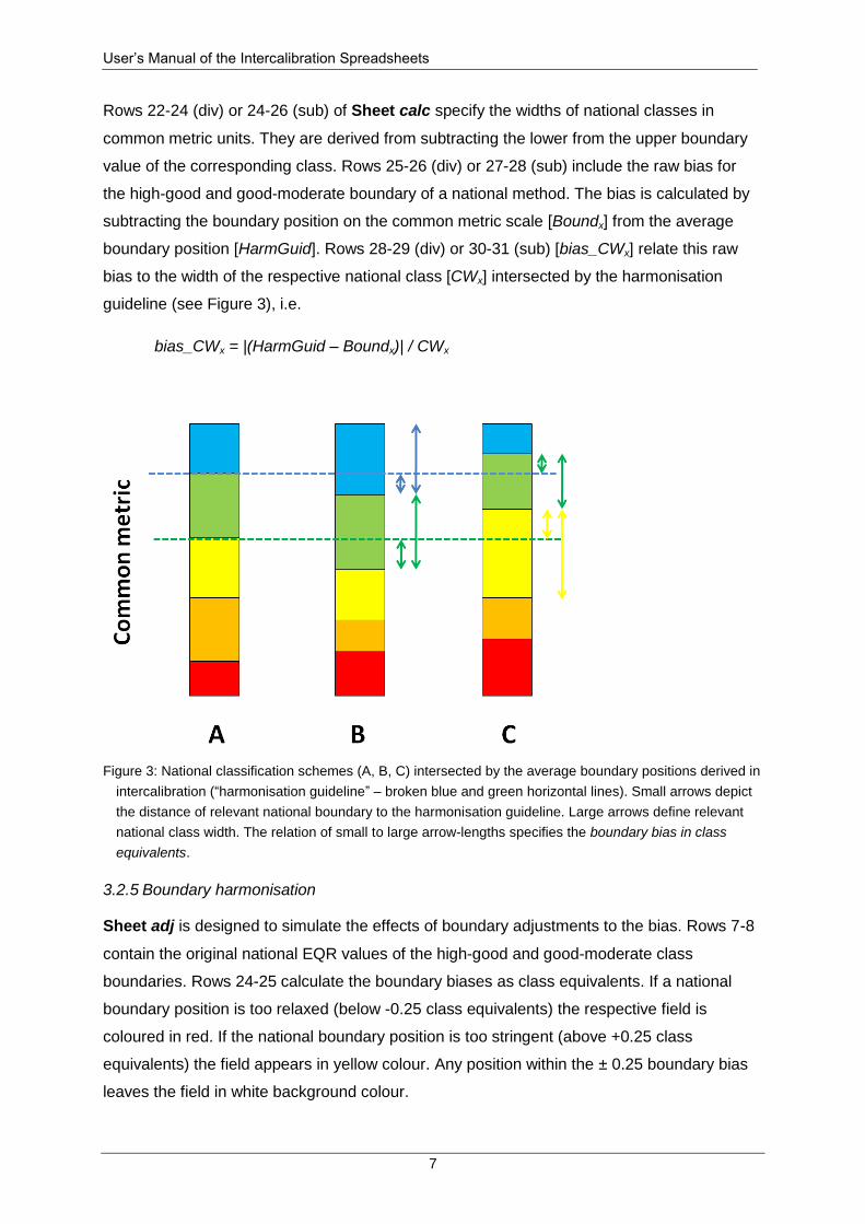
guideline (see Figure 3), i.e.
bias_CWx = |(HarmGuid – Boundx)| / CWx
Figure 3: National classification schemes (A, B, C) intersected by the average boundary positions derived in
intercalibration (“harmonisation guideline” – broken blue and green horizontal lines). Small arrows depict
the distance of relevant national boundary to the harmonisation guideline. Large arrows define relevant
national class width. The relation of small to large arrow-lengths specifies the boundary bias in class
equivalents.
3.2.5 Boundary harmonisation
Sheet adj is designed to simulate the effects of boundary adjustments to the bias. Rows 7-8
contain the original national EQR values of the high-good and good-moderate class
boundaries. Rows 24-25 calculate the boundary biases as class equivalents. If a national
boundary position is too relaxed (below -0.25 class equivalents) the respective field is
coloured in red. If the national boundary position is too stringent (above +0.25 class
equivalents) the field appears in yellow colour. Any position within the ± 0.25 boundary bias
leaves the field in white background colour.

User’s Manual of the Intercalibration Spreadsheets
8
You can now manually change the original boundary positions of any method and see the
effects on the boundary bias directly. The scheme uses the regression formulae and
benchmark definitions specified in the previous sheets. Note that the harmonisation guideline
(average boundary position of all methods) is not affected by the changes you make to this
sheet. For your convenience the original boundaries are displayed in rows 2-3.
Results are also presented in the diagrams on boundary bias (Figure 4).
Figure 4: Boundary bias expressed as class width equivalents per national method (diagram taken from
Sheet adj)
User’s Manual of the Intercalibration Spreadsheets
9
4 IC Option 3 spreadsheets
The basic features of calculating boundary bias are similar to the IC Option 2 spreadsheets
described above. The IC Option 3 spreadsheets additionally allow for the calculation of class
agreement. Note that the spreadsheets are only designed to follow IC Option 3a (see
CIS, 2010).
4.1 Input requirements
4.1.1 Sheet “Bm”
The reference values (usually “1.00”) and all national class boundaries (as EQR values)
need to be specified for each method participating in the intercalibration exercise (rows 3-7).
Select an appropriate identifier for the national methods as table headers.
Option 3 allows to identify up to 5 different subtypes per national method/country (see Birk &
Willby 2010). Specify the number of subtypes in row 8 and give different names to all these
subtypes in rows 9-13.
4.1.2 Sheet “data”
In IC Option 3 the intercalibration analyses are carried out on the basis of a common dataset
that includes samples commonly assessed by all methods participating in the exercise. The
spreadsheet on IC Option 3 requires information about:
Sample code
Country (origin of sample data)
Benchmark site (yes/no)8
Subtype (allocation of subtype to benchmark sites9; use the name(s) given in
Sheet Bm)
National EQRs headed by method identifier (starting from column E)
4.2 Steps of calculation
4.2.1 Linear regression against pseudo-common metric
The spreadsheet performs various calculation steps before establishing the linear
regressions (Figure 5). The raw values of the national EQRs are first benchmark
standardised (see section 4.2.2 for details). Then, the resulting values are normalised to a
range of 0-110. Out of these values the Pseudo-Common Metrics (PCM) are derived (average
8 Note that you must define benchmark sites for ALL subtypes.
9 only necessary for samples that belong to benchmark sites
10 Min-max normalisation

User’s Manual of the Intercalibration Spreadsheets
10
of all national EQRs per sample excluding the method to be compared against; see Willby &
Birk 2010). Finally, the regressions are established and displayed in Sheet reg. The graphs
include sample plots, regression formulae and R2 values. Note that at this stage benchmark
standardisation and normalisation have been applied to the data.
Sheet calc specifies details of the regressions (rows 8-12). Here, it is possible to manually
enter regression slopes for testing the effects of different slope values on the intercalibration
outcomes11.
Figure 5: Steps of the calculation before establishing linear regressions
4.2.2 Benchmark standardisation
Compared to IC Option 2 the process of benchmark standardisation is more complex. This is
because in Option 3 the assessment methods are applied to both foreign and national data12.
Therefore, each method is standardised individually for the different subtypes13 occurring in
the GIG (see Birk & Willby 2010).
11
This may be useful in cases of weak regressions (e.g. low number of samples, low R2 values).
12 An assessment method is adapted to regional conditions. It presumably performs best in the country of origin,
while applied outside its original range it is expected to yield less accurate results because it encounters
conditions or associations of species that differ from those of the sites on which it was trained.
13 Intercalibration subtypes are characterised by distinct biological communities that differ in taxonomic
composition and/or dominance structure. Subtypes occur within a common intercalibration type due to divers
patterns of species dispersal, climatological gradients or regional specificities of the common type (e.g., caused
by lithology, topography).

User’s Manual of the Intercalibration Spreadsheets
11
For each subtype (specified in the Sheets Bm and data) the spreadsheet calculates a
separate average (median) EQR of the national methods. These medians are then used for a
piece-wise standardisation for each set of subtype-data within a national method14. The
principle is exemplified in Figure 6. The median values per subtype used for the benchmark
standardisation are specified in Sheet calc (rows 14 and following).
Figure 6: Principle of benchmark standardisation as used by the spreadsheet (benchmark calculation:
division)
Benchmark calculation: Division15
As depicted in Figure 6 each national EQR value is divided by the median of the subtype the
sample belongs to. The standardised EQRs are listed in Sheets tdata and gdata (columns
headed by “sEQR”).
Benchmark calculation: Subtraction16
For each subtype’s benchmark sites the median EQRs of national methods are averaged
(Figure 7). To calculate the offset of each subtype the median values are then subtracted
from this average. The offset value differs between subtypes, so each subtype-dataset is
standardised by an individual offset value. The offsets per subtype and national method are
given in Sheet calc (rows 33 and following).
Each national EQR is added by the offset value of the subtype the sample belongs to. The
standardised EQRs are listed in Sheets tdata and gdata (columns headed by “sEQR”).
14
If several subtypes are occurring in one country the spreadsheet calculates the arithmetic mean of all subtype-
medians and uses this mean to standardise the national method applied to this country’s data. 15
Relevant for spreadsheet file IC_opt3_div.xls 16
Relevant for spreadsheet file IC_opt3_sub.xls
SampleSub-
typeBenchmark
National EQR
of Country A
National EQR
of Country B
Calculation:
EQR of Country A
Calculation:
EQR of Country B
Standardised
National EQR
Country A
Standardised
National EQR
Country B
S01 I Yes 0.97 0.80 1.11 1.00
S02 I Yes 0.82 0.78 0.94 0.98
S03 I Yes 0.87 0.99 1.00 1.24
S04 I No 0.54 0.65 0.62 0.81
S05 I No 0.73 0.34 0.84 0.43
S06 I No 0.34 0.21 0.39 0.26
S07 II Yes 0.89 0.99 1.00 1.27
S08 II Yes 0.76 0.76 0.85 0.97
S09 II Yes 0.99 0.78 1.11 1.00
S10 II No 0.43 0.54 0.48 0.69
S11 II No 0.32 0.43 0.36 0.55
S12 II No 0.12 0.22 0.13 0.28
National EQR of A
Median EQR of A at
Benchmark Sites of I
National EQR of A
Median EQR of A at
Benchmark Sites of II
National EQR of B
Median EQR of B at
Benchmark Sites of I
National EQR of B
Median EQR of B at
Benchmark Sites of II
Standardise the national EQR
for each subtype’s dataset in the common database individually
by dividing the actual EQR value of the sample by the median EQR value
at benchmark sites of the subtype from which the data originate.
*
* Example: 0.54 / 0.78 = 0.69

User’s Manual of the Intercalibration Spreadsheets
12
Figure 7: Scheme of the benchmark calculation: Subtraction for two national methods (A, B) assessing a
common dataset that includes three subtypes (I, II, III) (Ø: arithmetic mean of subtype medians; see text
for explanation)
4.2.3 Boundary translation
Reference values17 and boundaries are benchmark standardised and normalised before
being translated into PCM values. Modified references and boundaries are depicted in Sheet
calc [standardised values: rows 40-45 (div) or 58-63 (sub); standardised and normalised
values: rows 47-52 (div) or 65-70(sub)]. In the rows below these values are translated into
PCM units using the regressions specified in rows 8-12 (and displayed in Sheet reg).
4.2.4 Boundary bias
Boundary bias is one of the two components to check the comparability of national quality
classifications (CIS, 2010). Boundary bias is defined as the deviation of the relevant national
class boundary (high-good or good-moderate) from the average boundary position derived
from all methods participating in the exercise (“harmonisation guideline”). Boundary bias is
expressed in national class equivalents and must not exceed 0.25 units. All elements
required to calculate boundary bias are shown in Figure 8.
Rows 61-63 (div) or 79-81 (sub) of Sheet calc specify the widths of national classes high,
good and moderate in PCM units. They are derived from subtracting the lower from the
upper boundary value of the corresponding class. Rows 64-65 (div) or 82-83 (sub) include
the raw bias for the high-good and good-moderate boundary of each national method. The
bias is calculated by subtracting the boundary position on the PCM scale [Boundx] from the
average boundary position [HarmGuid]. Rows headed by [bias_CWx] relate this raw bias to
17
For the translation of the national reference value the spreadsheet uses either the reference given in Sheet Bm
or the highest EQR of the subtype for which the national method is designed (specified in Sheet data),
whichever is higher. This value is used for defining the width of the high status class (see following section).
SubtypeBenchmark sites assessed
by Method A
Average of medians at
benchmark sitesOffset
I MedianAI Ø - MedianAI
II MedianAII Ø - MedianAII
III MedianAIII Ø - MedianAIII
SubtypeBenchmark sites assessed
by Method B
Average of medians at
benchmark sitesOffset
I MedianBI Ø - MedianBI
II MedianBII Ø - MedianBII
III MedianBIII Ø - MedianBIII
Ø
Ø
User’s Manual of the Intercalibration Spreadsheets
13
the width of the respective national class [CWx] intersected by the harmonisation guideline
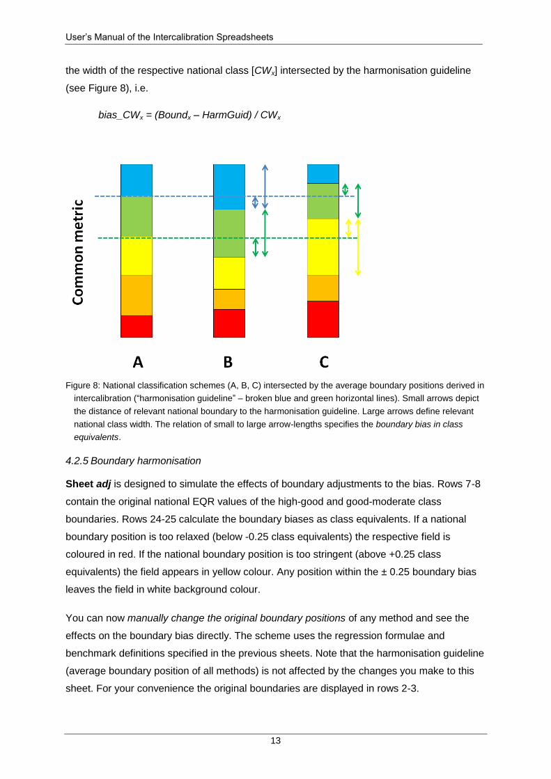
(see Figure 8), i.e.
bias_CWx = (Boundx – HarmGuid) / CWx
Figure 8: National classification schemes (A, B, C) intersected by the average boundary positions derived in
intercalibration (“harmonisation guideline” – broken blue and green horizontal lines). Small arrows depict
the distance of relevant national boundary to the harmonisation guideline. Large arrows define relevant
national class width. The relation of small to large arrow-lengths specifies the boundary bias in class
equivalents.
4.2.5 Boundary harmonisation
Sheet adj is designed to simulate the effects of boundary adjustments to the bias. Rows 7-8
contain the original national EQR values of the high-good and good-moderate class
boundaries. Rows 24-25 calculate the boundary biases as class equivalents. If a national
boundary position is too relaxed (below -0.25 class equivalents) the respective field is
coloured in red. If the national boundary position is too stringent (above +0.25 class
equivalents) the field appears in yellow colour. Any position within the ± 0.25 boundary bias
leaves the field in white background colour.
You can now manually change the original boundary positions of any method and see the
effects on the boundary bias directly. The scheme uses the regression formulae and
benchmark definitions specified in the previous sheets. Note that the harmonisation guideline
(average boundary position of all methods) is not affected by the changes you make to this
sheet. For your convenience the original boundaries are displayed in rows 2-3.
User’s Manual of the Intercalibration Spreadsheets
14
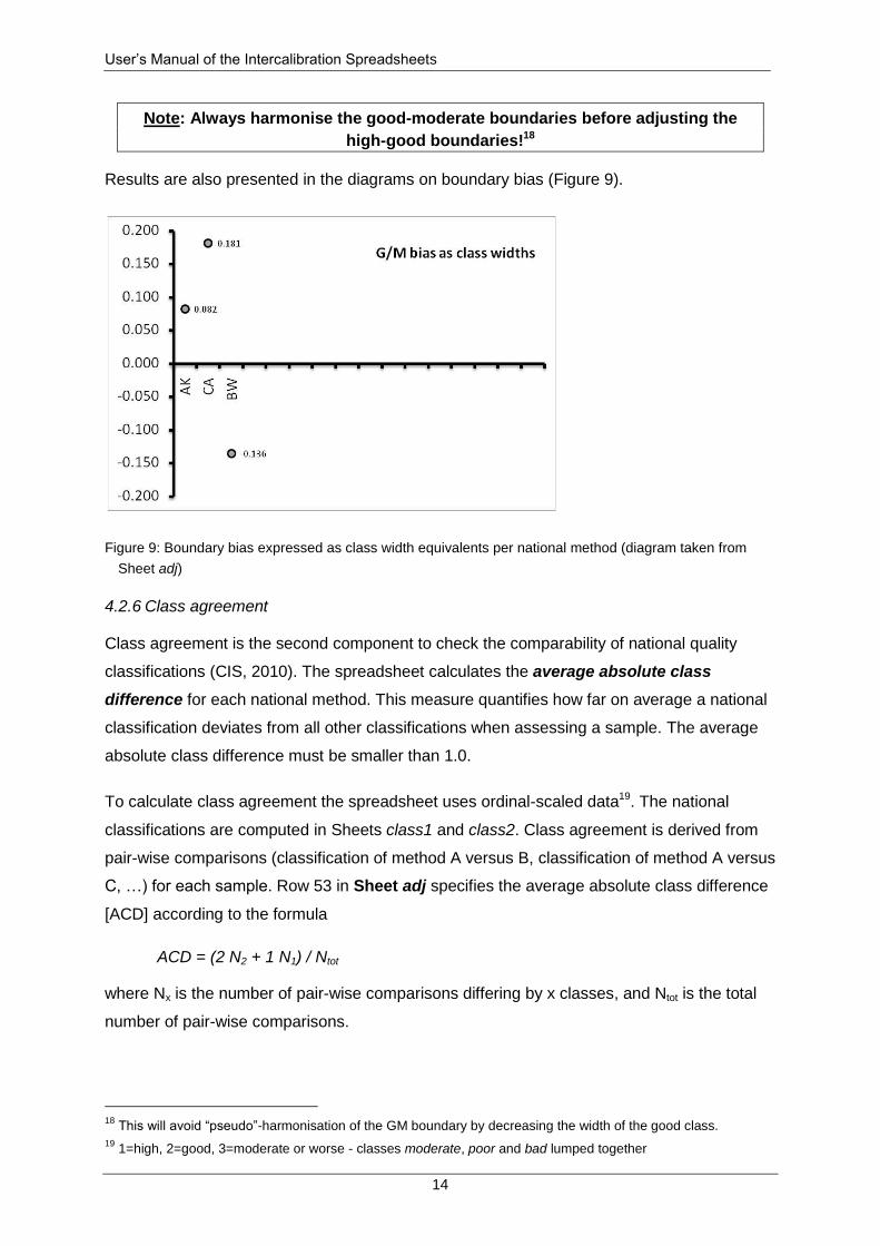
Note: Always harmonise the good-moderate boundaries before adjusting the
high-good boundaries!18
Results are also presented in the diagrams on boundary bias (Figure 9).
Figure 9: Boundary bias expressed as class width equivalents per national method (diagram taken from
Sheet adj)
4.2.6 Class agreement
Class agreement is the second component to check the comparability of national quality
classifications (CIS, 2010). The spreadsheet calculates the average absolute class
difference for each national method. This measure quantifies how far on average a national
classification deviates from all other classifications when assessing a sample. The average
absolute class difference must be smaller than 1.0.
To calculate class agreement the spreadsheet uses ordinal-scaled data19. The national
classifications are computed in Sheets class1 and class2. Class agreement is derived from
pair-wise comparisons (classification of method A versus B, classification of method A versus
C, …) for each sample. Row 53 in Sheet adj specifies the average absolute class difference
[ACD] according to the formula
ACD = (2·N2 + 1·N1) / Ntot
where Nx is the number of pair-wise comparisons differing by x classes, and Ntot is the total
number of pair-wise comparisons.
18
This will avoid “pseudo”-harmonisation of the GM boundary by decreasing the width of the good class.
19 1=high, 2=good, 3=moderate or worse - classes moderate, poor and bad lumped together

User’s Manual of the Intercalibration Spreadsheets
15
We advice to follow a “One out - all out” principle when judging acceptability of comparisons,
i.e. for any method not meeting the criterion intercalibration has failed. Note that class
agreement is tested after adjusting the boundary bias (i.e. boundary harmonisation).

User’s Manual of the Intercalibration Spreadsheets
16
5 References
Birk S, Willby NJ (2010) The definition of alternative benchmarks in intercalibration – outline
of general procedure and case study on river macrophytes. Final report commissioned
by JRC Ispra. Essen and Stirling.
CIS (Common Implementation Strategy) (2010) Guidance document on the intercalibration
process 2008-2011. Guidance Document No. 14. Implementation Strategy for the
Water Framework Directive (2000/60/EC). Brussels.
Willby NJ, Birk S (2010) Definition of comparability criteria for setting class boundaries -
Outline of the procedure to compare and harmonise the national classifications of
ecological status according to the WFD intercalibration exercise. Final report
commissioned by JRC Ispra. Stirling and Essen.
Recommended