Usefulness of single nucleotide polymorphism (SNP) data for estimating
population parameters
Mary K. Kuhner, Peter Beerli, Jon Yamato and Joseph Felsenstein
Department of Genetics, University of Washington
1
Running title: SNP-based parameter estimation
Keywords: single nucleotide polymorphisms, maximum likelihood, parameter
estimation, Metropolis-Hastings algorithm, recombination
Corresponding author:
Mary K. Kuhner
Department of Genetics
University of Washington
Box 357360
Seattle, WA 98195-7360, USA.
Telephone (206) 543-8751
FAX (206) 543-0754
email [email protected]
2
ABSTRACT
Single nucleotide polymorphism (SNP) data can be used for parameter
estimation via maximum likelihood methods as long as the way in which the
SNPs were determined is known, so that an appropriate likelihood formula can be
constructed. We present such likelihoods for several sampling methods. As a test
of these approaches, we consider use of SNPs to estimate the parameter Θ = 4Neµ
(the scaled product of effective population size and per-site mutation rate), which is
related to the branch lengths of the reconstructed genealogy. With infinite amounts
of data, ML models using SNP data are expected to produce consistent estimates
of Θ. With finite amounts of data the estimates are accurate when Θ is high,
but tend to be biased upwards when Θ is low. If recombination is present and
not allowed for in the analysis, the results are additionally biased upwards, but
this effect can be removed by incorporating recombination into the analysis. SNPs
defined as sites which are polymorphic in the actual sample under consideration
(sample SNPs) are somewhat more accurate for estimation of Θ than SNPs defined
by their polymorphism in a panel chosen from the same population (panel SNPs).
Misrepresenting panel SNPs as sample SNPs leads to large errors in the maximum
likelihood estimate of Θ. Researchers collecting SNPs should collect and preserve
information about the method of ascertainment so that the data can be accurately
analyzed.
INTRODUCTION
Modern population genetics methods require large samples of population level
genetic information in order to answer questions about population size, migration,
selection, and other factors. Many researchers have recently begun collecting single
3
nucleotide polymorphism (SNP) data in the hopes of addressing these questions,
as well as for their applications in gene mapping (for an overview, see Syvanen et
al. 1999). This paper examines methods for analyzing SNP data in a maximum
likelihood (ML) framework.
Appropriate analysis of SNPs depends on knowing how they were collected.
Critical pieces of information include:
(1) Were candidate sites chosen from completely linked, partially linked, or
unlinked regions of the genome?
(2) Were sites defined as SNPs based on their polymorphism in the sample at
hand, a panel drawn from the same population, or a panel drawn from a different
population?
As one possible measure of the usefulness of SNP data, we will consider the
estimation of the parameter Θ = 4Neµ, four times the product of the effective
population size and the neutral mutation rate. We will look at the simple case of
a single random-mating diploid population of constant effective population size Ne.
At each site, selectively neutral mutations occur with probability µ per generation.
This parameter will be estimated using the Metropolis-Hastings method of
Kuhner et al. (1995) which samples among possible coalescent trees describing the
relationship among the sampled sequences according, in part, to their likelihood
under a given model of sequence evolution. The information about Θ is specifically
found in the branch lengths of the sampled trees: therefore, estimation of Θ
indirectly tests the ability of a SNP likelihood model to accurately estimate branch
lengths.
We test the effect of both unacknowledged and acknowledged recombination
on the accuracy of these estimates, since SNP data will often come from a context
where recombination is possible.
4
The use of SNP data to estimate parameters not closely related to branch
length, such as tree topology and map order, will be considered in a future paper.
It seems likely that SNP data will be more powerful for such parameters than they
are for branch lengths; however, the pitfalls found here will probably be found in
those areas as well.
METHODS
Likelihood framework for SNPs: The estimation of phylogenies by
maximum likelihood from DNA sequences (Felsenstein 1981) computes, for each site,
the probability of that site on a given phylogeny: this we call the site likelihood.
The likelihood of the entire data set on the given phylogeny is the product of the
site likelihoods.
To analyze SNPs using this approach, several aspects of the way the SNPs
were collected must be taken into consideration: this is analogous to considering
ascertainment of individuals in a case/control disease study.
In the first section we will consider the question of whether the SNPs were
gathered from a single completely linked region, from various unlinked locations, or
from a linked region with some internal recombination. In the following section we
will consider the question of whether the SNPs were defined based on polymorphism
in the sample or in a panel. These sections define a toolkit from which SNP
corrections for many specific cases can be constructed. Table 1 gives an overview of
the issues and the appropriate means of analysis for each set of conditions.
Linkage considerations: At one extreme, candidate sites could be drawn
from a single, non-recombining stretch of DNA and evaluated to find SNPs. In this
case all of the SNPs, as well as the unobserved sites around them, would have the
same underlying coalescent genealogy. We will call this case “fully linked SNPs.” At
5
the other extreme, candidate sites could be chosen at random from a recombining
genome in such a way that successive draws represent completely independent
coalescent genealogies (“unlinked SNPs”). Between these extremes, successive
candidates will represent correlated, but not always identical, coalescent genealogies:
this is the case for long sequences taken from a genome with recombination, and we
will call it “partially linked SNPs.”
An additional consideration is whether any information at all is available on the
number of sites not selected as SNPs. Some methods of data collection–for example,
using anonymous probes to detect SNPs– will not give us any information on how
many “unobserved” sites were in the region of interest. Other methods–for example,
choosing SNPs from a region of known length–will allow us to determine this. As
will be shown, if this information is available it allows us to use alternative methods
of constructing the likelihood, and in the case of recombination it allows analysis of
otherwise intractable data.
We will first consider the case where information is available only on the SNPs
themselves. Here, we modify the usual DNA likelihood model by conditioning on
the site being a SNP (by whatever criteria are in use), an event with probability
P (SNP|G). The difference between analysis of linked and unlinked SNPs lies in
the choice of genealogies to consider. This approach will be referred to as the
“conditional likelihood” method. It is closely related to work done by Ewens et al.
(1981) on parameter estimation using RFLPS.
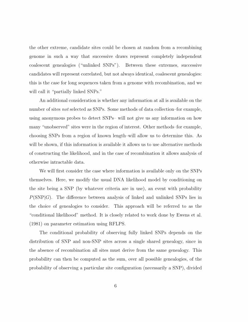
The conditional probability of observing fully linked SNPs depends on the
distribution of SNP and non-SNP sites across a single shared genealogy, since in
the absence of recombination all sites must derive from the same genealogy. This
probability can then be computed as the sum, over all possible genealogies, of the
probability of observing a particular site configuration (necessarily a SNP), divided
6
by the probability that a given site is a SNP. The product is over all SNP sites.
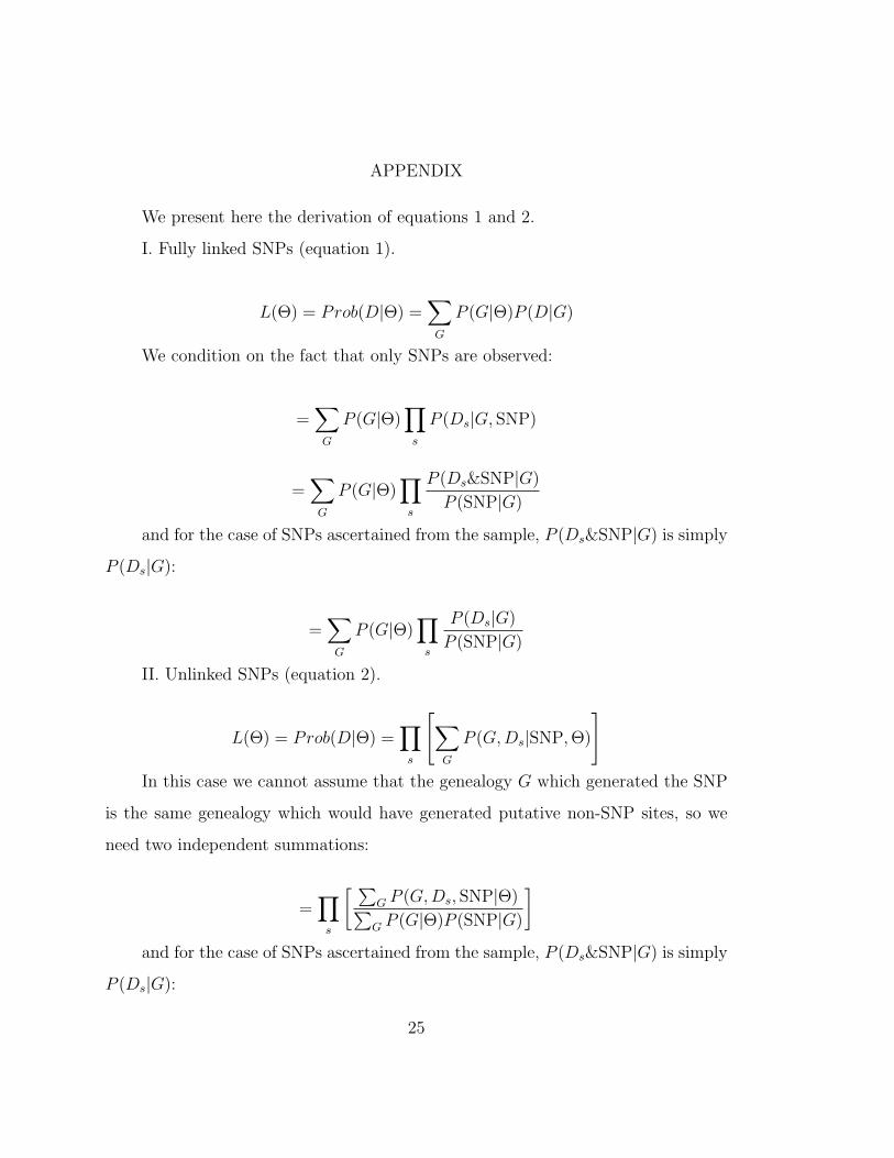
(The derivation of this equation is given in more detail in the Appendix.)
L(Θ) =∑
G
P (G|Θ)∏
s
P (Ds|G)
P (SNPs|G)(1)
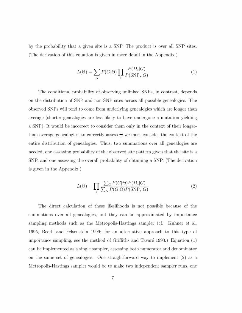
The conditional probability of observing unlinked SNPs, in contrast, depends
on the distribution of SNP and non-SNP sites across all possible genealogies. The
observed SNPs will tend to come from underlying genealogies which are longer than
average (shorter genealogies are less likely to have undergone a mutation yielding
a SNP). It would be incorrect to consider them only in the context of their longer-
than-average genealogies; to correctly assess Θ we must consider the context of the
entire distribution of genealogies. Thus, two summations over all genealogies are
needed, one assessing probability of the observed site pattern given that the site is a
SNP, and one assessing the overall probability of obtaining a SNP. (The derivation
is given in the Appendix.)
L(Θ) =∏
s
∑G P (G|Θ)P (Ds|G)∑
G P (G|Θ)P (SNPs|G)(2)
The direct calculation of these likelihoods is not possible because of the
summations over all genealogies, but they can be approximated by importance
sampling methods such as the Metropolis-Hastings sampler (cf. Kuhner et al.
1995, Beerli and Felsenstein 1999; for an alternative approach to this type of
importance sampling, see the method of Griffiths and Tavare 1993.) Equation (1)
can be implemented as a single sampler, assessing both numerator and denominator
on the same set of genealogies. One straightforward way to implement (2) as a
Metropolis-Hastings sampler would be to make two independent sampler runs, one
7
sampling from the numerator, one from the denominator. There may be a more
economical approach where a single sample of genealogies is adequate to estimate
both numerator and denominator.
The case of partial linkage, where successive sites have correlated genealogies,
is more difficult. It may in fact be impossible to solve without information about
the number and location of unobserved sites. The difficulty is that the unobserved
sites are drawn from a distribution which is correlated with, but not identical to, the
distribution of the observed SNPs. Without knowing this distribution, we cannot
construct an appropriate correction.
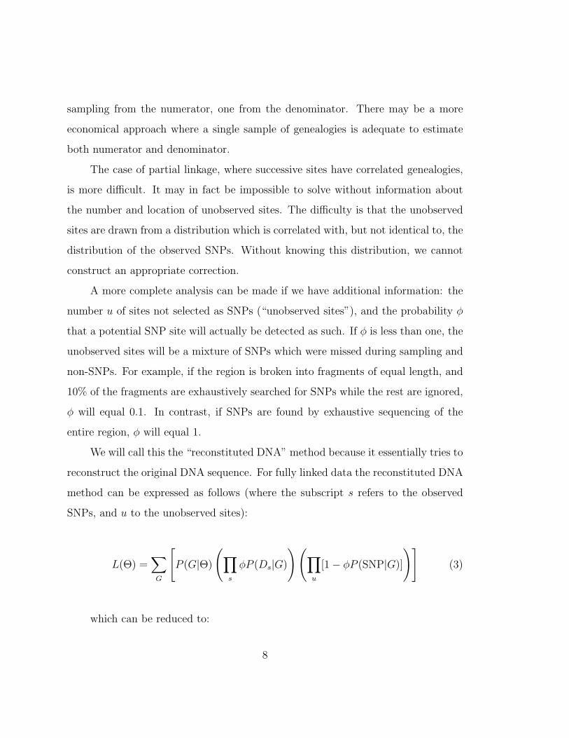
A more complete analysis can be made if we have additional information: the
number u of sites not selected as SNPs (“unobserved sites”), and the probability φ
that a potential SNP site will actually be detected as such. If φ is less than one, the
unobserved sites will be a mixture of SNPs which were missed during sampling and
non-SNPs. For example, if the region is broken into fragments of equal length, and
10% of the fragments are exhaustively searched for SNPs while the rest are ignored,
φ will equal 0.1. In contrast, if SNPs are found by exhaustive sequencing of the
entire region, φ will equal 1.
We will call this the “reconstituted DNA” method because it essentially tries to
reconstruct the original DNA sequence. For fully linked data the reconstituted DNA
method can be expressed as follows (where the subscript s refers to the observed
SNPs, and u to the unobserved sites):
L(Θ) =∑
G
[P (G|Θ)
(∏s
φP (Ds|G)
)(∏u
[1 − φP (SNP|G)]
)](3)
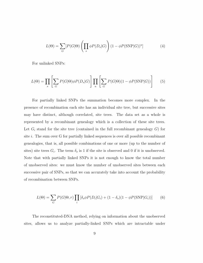
which can be reduced to:
8
L(Θ) =∑
G
[P (G|Θ)
(∏s
φP (Ds|G)
)(1 − φP (SNP|G))u] (4)
For unlinked SNPs:
L(Θ) =∏
s
[∑G
P (G|Θ)φP (Ds|G)
]∏u
[∑G
P (G|Θ)(1 − φP (SNP|G))
](5)
For partially linked SNPs the summation becomes more complex. In the
presence of recombination each site has an individual site tree, but successive sites
may have distinct, although correlated, site trees. The data set as a whole is
represented by a recombinant genealogy which is a collection of these site trees.
Let Gi stand for the site tree (contained in the full recombinant genealogy G) for
site i. The sum over G for partially linked sequences is over all possible recombinant
genealogies, that is, all possible combinations of one or more (up to the number of
sites) site trees Gi. The term δo is 1 if the site is observed and 0 if it is unobserved.
Note that with partially linked SNPs it is not enough to know the total number
of unobserved sites: we must know the number of unobserved sites between each
successive pair of SNPs, so that we can accurately take into account the probability
of recombination between SNPs.
L(Θ) =∑
G
P (G|Θ, r)∏
i
[δoφP (Di|Gi) + (1 − δo)(1 − φP (SNP|Gi))] (6)
The reconstituted-DNA method, relying on information about the unobserved
sites, allows us to analyze partially-linked SNPs which are intractable under
9
the conditional-likelihood method. This approach can be incorporated into a
recombination-aware Metropolis-Hastings sampler (Kuhner et al. submitted). The
resulting search among genealogies considers both the site trees which actually
yielded SNPs and other site trees, interspersed among them, which did not.
A specialized case worth considering is the one in which short chunks of DNA
from well separated locations are searched for SNPs. If the chunks are short and
recombination is infrequent, it may be reasonable to treat such chunks as fully
linked internally and completely unlinked with one another. They can then be
analyzed under the reconstituted-DNA model using a combination of equation 4
(within chunks) and the logic for combining multiple unlinked loci in an MCMC
sampler described in Kuhner et al. 1995, as long as the length of each chunk is
known.
The conditional-likelihood approach could also be used if the number of SNPs
sampled from one chunk were independent of the density of SNPs in that chunk
(for example, if the researcher examined each chunk until 5 SNPs were found and
then stopped). However, in the more usual case where all SNPs in the chunk are
reported, straightforward application of the conditional-likelihood approach leads
to a bias. Chunks with a deep genealogy produce many SNPs, and the likelihood
curves from such chunks are therefore well defined. Chunks with a shallow genealogy
produce few SNPs and a relatively flat likelihood curve. The deeper genealogies will
thus dominate the combined estimate, leading to an overestimate of Θ. It may be
possible to overcome this effect with an appropriate conditioning on the number of
SNPs in each chunk, but the reconstituted-DNA approach seems simpler–in effect
it does the necessary conditioning automatically.
Methods of defining a SNP: The next question of interest is how a candidate
site is determined to be a SNP once it is drawn. There are at least three possibilities.
10
The site might be classified as a SNP because it is polymorphic in the actual sample
under consideration (“sample SNPs”); because it is polymorphic in a panel drawn
from the same population (“panel SNPs”); or because it is polymorphic in a panel
from a different, though presumably related, population (“different-population panel
SNPs”).
We consider a site to be polymorphic if at least one nucleotide difference is seen.
More restricted definitions, such as “a site is polymorphic if the frequency of the
most common allele is less than 0.95,” can in principle be handled by modifications
of these approaches.
The terms we need to consider are the sitewise data likelihoods P (D&SNP|G)
(the probability that a site of a given configuration D will be obtained as a SNP)
and P (SNP|G) (the probability that a site will be a SNP). It will be useful to define
I as an invariant site, Ip as a site which is invariant in the panel, and Is as a site
which is invariant in the sample.
Sample SNPs: Here the data contain only polymorphic sites by definition,
and the data likelihood P (D&SNP|G) reduces to P (D|G) since the conditional
probability that the observed site is polymorphic is 1. This likelihood can be
calculated as a standard DNA likelihood (Felsenstein 1981) on the site’s genealogy.
The term P (SNP|G) can most readily be calculated as 1 − P (Is|G), where Is is
the sum of the probabilities that the site has all A’s, all C’s, all G’s, or all T’s on
the given genealogy. An analogous correction was used by Felsenstein (1992) for
restriction fragment length polymorphism data.
Panel SNPs: Here the genealogy G must be widened to include relationships
not only among the sampled individuals, but among the panel individuals and
between panel and sample individuals. We assume that as long as a site is found to
vary in the panel, it will be included in our calculation even if it proves not to vary
11
in the sample, since this will generally not be known until after the data is collected.
The method can readily be modified to cover the case where sites that prove to be
invariant in the sampled individuals are discarded, but this should be avoided if at
all possible, as it loses information unnecessarily.
We will call the data for a given site in the actual sample Ds and the data
for that site in the panel Dp. If Dp is known, we should merge panel and sample
together, transforming the data into sample SNPs. Often, however, all we will know
is that Dp was not invariant. The term P (D&SNP|G) can then be written as the
probability of observing Ds given that the site is variable in the panel, which is
equal to the probability of Ds minus the probability of cases in which the panel
was invariant: P (Ds|G)−P (Ds&Ip|G). This is somewhat cumbersome to bookkeep
in a Metropolis-Hastings context, but presents no theoretical difficulties. It will,
however, slow such an analysis by increasing the size of the search space, since G
must now include the possible genealogy of the panel as well as the sample.
Different-population panel SNPs: This case is more demanding, as the
genealogy G which relates sample and panel must take into account the relationship
between the two populations. If this relationship is basically that of two static
populations undergoing migration, an appropriate method would be to use the logic
of Migrate (Beerli and Felsenstein 1999) to construct a Metropolis-Hastings sampler
across multi-population genealogies with migration. These migration genealogies
could then be used in the same types of equations as for same-population sample
SNPs. Such an analysis would be much more effective if Dp were known, but
would have some power even if it were unknown, since tests of Migrate have
shown that it has some ability to infer parameters from a subpopulation for which
no data are given (P. Beerli, unpublished). We are in the process of developing
such a sampler. Migrate can analyze multiple sub-populations, and so that in
12
theory a complex relationship between panel and sample subpopulations could be
accomodated, although a large amount of data might be required. The closer the
relationships among the subpopulations, the more informative such data will be.
If the relationship between the two populations is common descent from an
ancestral population, a Metropolis-Hastings sampler incorporating this relationship
could also be constructed. There is currently no practical experience to tell us how
much power would be available to such a sampler, though unless the separation of
the populations is recent relative to the age of the mutations causing the SNPs,
many of the SNP sites defined on the panel may be uninformative on the sample.
It is clear that if the approach used to define the SNPs is not known, there is
not enough information available to construct a full likelihood method.
Consistency of estimation with SNPs:
In this section we investigate whether SNP data can be used to make a
consistent ML reconstruction of the tree, since if the coalescent tree can be
reconstructed consistently, a consistent estimate of Θ will naturally follow.
Maximum likelihood phylogeny reconstruction from DNA data can be shown
to be consistent when a correct model of sequence evolution is used (Chang 1996).
Consistency means that the estimate converges to the correct solution (both topology
and branch lengths) as the amount of data becomes infinite. Since the SNP
likelihood model is derived from the full DNA model, it may also be consistent,
but we must consider whether loss of information about the non-SNP sites causes
inconsistency.
It is immediately apparent that the conditional-likelihood approach will fail in
some cases where DNA (or reconstituted DNA) estimation would succeed. Consider
unlinked sites from two individuals and a Jukes-Cantor model (Jukes and Cantor
1969) of sequence evolution. The full DNA model can consistently estimate the
13
branch length separating the two individuals, but to do so it relies on comparing the
frequency of invariant sites (sites of pattern xx) with the frequency of variable sites
(pattern xy). To make SNP data we discard all sites of pattern xx leaving ourselves
with no information: the remaining xy sites are expected with probability 1 for any
non-zero value of the branch length. (If the branch length were zero we would have
come back empty-handed from our search for SNPs.)
However, with three or more individuals sufficient information is available with
SNP data even if the number of unobserved sites is not known. For unlinked SNPs,
three individuals allow the possibility of site classes xxy and xyz (for unlinked SNPs
possibilities such as xyx are equivalent to xxy). Using the Jukes-Cantor model
we can derive (by taking the expectation of the multinomial sampling probability
over the distribution of allele frequencies in a symmetrical four-allele model, as in
Watterson (1977)) an expression for the proportion of xxy sites as a function of Θ:
Pxxy
Pxxy + Pxyz
=3 + 3Θ
3 + 5Θ
This function is monotonically decreasing in Θ and thus any value of the ratio
corresponds to a unique estimate of Θ. We believe, although it is difficult to show
analytically, that the same is true for linked SNPs where the actual genealogy is being
estimated. Since the genealogy has multiple parameters, more information is needed,
but more is available since classes xxy, xyx and yxx can now be distinguished.
It should be noted that if the model of DNA evolution used to derive the site-
class expectations is not identical to the one which governed the actual generation
of the data, there is no guarantee that the maximum likelihood estimate will be
consistent. (This is not a flaw in likelihood analysis: no method can be expected to
be consistent if it is based on an incorrect model.) However, as long as three or more
sequences are sampled, properly conditioned maximum likelihood analysis of SNPs
14
should be consistent under the same conditions as maximum likelihood analysis of
the underlying DNA data.
Bias of estimation with SNPs: It would be natural to ask whether
estimation of Θ using finite amounts of SNP data is biased: that is, what is the
expectation of the estimate with finite data? Surprisingly enough, however, the
mean bias is infinite for both SNP data and full DNA data. For both SNPs and full
DNA data there exist possible data configurations for which the estimate of Θ is
infinite. Thus the expectation is a mean over terms some of which are infinite, and
the mean bias must be infinite.
At first this seems very alarming. However, the cases which give an infinite
estimate are extremely unlikely with reasonably sized data sets (more than 5-10
sites), and for the vast majority of data sets a good estimate is produced. This
suggests that if we want practical guidance as to whether the method is working
well in a particular case, simulations are still relevant, even though we expect that
if enough simulations were performed the mean estimate would be infinite.
Even in the absence of infinitely large estimates, we expect an upward tendency
in the results of estimations using SNPs. In the tree of three tips, all of the
information is in the ratio of xxy to xyz sites. Sites of the xyz class are rare
for reasonable values of Θ (cases where they are not rare are unlikely to come up
in biological practice, since they would represent DNA so divergent that homology
and alignment would become problematic). Since they are rare, their frequency
will be poorly estimated by small data sets. The relationship between fxyz and the
estimate of Θ is non-linear, with upwards deviations in fxyz producing a much larger
effect than downwards ones. If we estimate f(xyz) with error that is symmetrically
distributed around the true value, we expect an upwards tendency in our results.
The full DNA model is not as vulnerable to this effect because it is not solely
15
dependent on f(xyz) for its information: the proportion of sites which are xxx is
also informative, and since they are common, much more information is available.
In the simulation section, we provide some empirical exploration of the amount
of SNP data needed to get an accurate estimate.
Computer simulations: Random coalescent trees for a given value of Θ,
and recombining-coalescent trees for given values of Θ and r, were made using a
program provided by Richard Hudson (personal communication). DNA data were
simulated on these trees using a modification of the program treedna (Felsenstein,
unpublished) which uses the Kimura 2-parameter model (Kimura 1980). We set the
transition/transversion ratio to 2.0 representing a moderate transition bias, such as
might be expected from the nuclear DNA of mammals.
To create sample SNP data we simulated trees containing the desired number
of tips (sequences), and recorded all polymorphic sites generated. To create panel
SNP data we simulated trees containing a number of tips equal to the sum of panel
and sample sizes, and then chose the panel out of these tips at random. The panel
was used to determine which sites to sample, and these sites were then sampled
from the remaining tips, even if they were not polymorphic among those tips.
Data from the panel individuals were then discarded. This method is appropriate
because a coalescent tree generated for a given number of individuals is statistically
indistinguishable from one generated for the entire population and then subsampled
to give that number of individuals.
The parameter φ (the chance that, if a site were eligible to be a SNP, it would
be detected as one) was set to 1.
Estimates of Θ were made using the program Recombine from the LAMARC
package (http://evolution.genetics.washington.edu/lamarc.html). Recombine is an
extension of Coalesce (Kuhner et al. 1995). For analysis of completely linked SNPs
16
we fixed the value of the recombination parameter r (equal to ρ/µ where ρ is the
recombination rate per site per generation and µ is the mutation rate per site per
generation) at zero; for analysis of partially linked SNPs we tested the program
both with and without co-estimation of r. Like Coalesce, Recombine samples over
a variety of trees in proportion to how well they fit the data, and uses these trees to
make an overall estimate of its parameters. In this case, the distribution of branch
lengths among the sampled trees is used to make a maximum likelihood estimate of
Θ and, optionally, r.
The program runs a series of Markov chains that sample these coalescent trees.
From the sample of trees in each chain, a new estimate of the parameters is made:
this estimate in turn provides a starting point for the next chain. Finally, a longer
chain is run to produce the final estimate. In this study, for each estimation we ran
10 short chains of 500 trees each and 1 long chain of 10,000 trees, sampling every
20th tree. The program was provided with the correct nucleotide frequencies and
transition/transversion ratio for the DNA model used.
Some data sets did not contain any variable sites. Rather than attempting to
make an estimate of Θ in these cases, we assigned the obvious estimate of zero. (The
Recombine program would move towards an estimate of zero, but would encounter
problems such as arithmetic underflow before actually arriving there.)
To test whether the presence of some recombination in the sequences disrupts
the estimate, we created sequences with various levels of recombination, and
analyzed them with and without co-estimating recombination.
RESULTS
We did not explore the case of unlinked SNPs. The Metropolis-Hastings
sampler is overkill on such data, since single unlinked sites do not provide enough
17
information for any kind of tree estimate. An analytic solution may be possible if
the mutational model is not too complex.
As expected, representing SNPs as DNA leads to drastic overestimation of Θ
(Table 2A and 2B, line 1).
For fully linked SNPs, when Θ was quite high (0.1) both sample SNPs and panel
SNPs gave estimates close to the truth and had similar standard deviations (Table
2A lines 2 and 4). The standard deviations were about twice as high as observed
in Kuhner et al. (1998) using the full DNA model for a similar case (although that
case involved estimation of growth rate as well as Θ). Use of reconstituted DNA led
to standard deviations nearly as good as those from the full DNA model (Table 2A
lines 3 and 5).
When panel SNPs were misrepresented as sample SNPs, the estimates were
approximately tenfold too low (Table 2A line 6). In this high-Θ case, both sample
and panel SNPs can be successful at recovering Θ, but only if the method of
ascertainment is correctly specified. Why is incorrect specification so disastrous?
Mislabelling panel SNPs as sample SNPs forces us to discard sites which are found
to be invariant in the sample, reducing the amount of available data, but this is not
the main reason for the poor results: if it were, results with 1000 bp of DNA and
mislabelled SNPs (yielding an average of 180 analyzable sites) should be superior to
results with 500 bp of DNA and panel SNPs (yielding an average of 118 analyzable
sites). In fact they were much inferior. The fundamental problem is that panel
SNPs are depleted for variable sites arising from mutations in tipwards branches,
since such sites will not be shared between panel and sample members: analysing
them as sample SNPs ignores this depletion, leading to misinterpretation of the
data.
Use of reconstituted DNA reduced the size of this error, leading to estimates
18
which were about 60% of the true value (Table 2A line 7).
For our lower value of Θ (0.01), which is still quite high by biological standards,
the results (Table 2B) were less encouraging. Even with correct labelling, sample
SNPs overestimated Θ by a factor of about 2, and panel SNPs by a factor of about 3.
The standard deviations were approximately 10 times higher than would have been
obtained with use of the full DNA model (compare with Table 1 of Kuhner et al.
1995). Reconstituted DNA improved the sample-SNP estimates, as did increasing
the number of base pairs: with 1000 bp of reconstituted DNA the estimate was
nearly correct.
The results with mislabelled data at the lower Θ were again drastically too low,
and again, reconstituted DNA appeared to improve the situation but not to produce
a correct estimate. The high result for the case with 500 bp and R-Mislabelled
SNPs is the mean of many results lower than the truth and a single extremely high
estimate, and probably does not indicate a repeatable upwards tendency.
Table 3 shows the result of ignoring recombination when it is present. The
higher the recombination parameter r, the more severe the upwards bias in Θ.
Between-site nconsistencies that are introduced by recombination must, in a no-
recombination model, be interpreted as multiple mutations, inflating the estimate.
Table 4 shows that when recombination is explicitly modelled, only a slight
upward bias in Θ remains. It is especially striking that allowing for recombination
improves the estimate of Θ (compare Table 3 and Table 4) even when there is clearly
insufficient information to allow a good estimate of the recombination parameter r
itself. (Our experience of the Recombine program is that it cannot make accurate
estimates of r on such short sequences.)
DISCUSSION
19
When Θ is relatively low, estimates based on SNP data will be inaccurate
because site patterns other than the most common one will be very infrequent,
and thus their frequency will be poorly estimated. In such cases, a method which
assumes an infinite-sites model and estimates a per-locus rather than per-site 4Neµ,
such as the methods of Watterson (1975), Griffiths and Tavare (1993) or Nielsen
(personal communication) may be preferable. Sampling greater numbers of SNPs
will slowly improve this situation, but for low values of Θ extremely large numbers
of SNPs will be required.
However, when Θ is relatively high accurate estimates are possible, though at
some loss of efficiency compared to use of the full DNA model. In cases where SNP
data is less expensive to collect than full DNA data this trade-off may be worthwhile.
Somewhat surprisingly, a panel of ten individuals appears sufficient, in the high-Θ
case, to give results nearly as good as those obtained by choosing SNPs from the
sample itself.
Intuitively one might expect that considering only the “informative” variable
sites from a piece of DNA would preserve most of its information value. While this
may be true for estimation of tree topology, it is not true for estimation of Θ or other
parameters that are based on branch lengths. Much of the lost information can be
recovered by the reconstituted-DNA approach, though this will be subject to errors
if the estimate of φ is incorrect or the SNPs are for some reason not characteristic
of the sequence in which they are embedded.
If there is any chance that recombination is present, a model which allows for
recombination will produce more accurate estimates of Θ than one which denies it;
the gain due to better matching of model to reality appears to easily offset the cost
of estimating an additional parameter.
Of the two models we present, conditional-likelihood and reconstituted-DNA,
20

the conditional-likelihood method is simpler and requires less additional information,
but it appears less accurate and cannot be extended to cases in which there is some
recombination. The reconstituted-DNA approach appears preferable whenever a
reasonable guess can be made about the frequency of SNPs in the unobserved sites.
An important additional question is whether SNPs will be fully informative for
gene mapping by coalescent-based methods. On theoretical grounds we believe that
an accurate SNP likelihood model will be important in obtaining good gene-mapping
results: while use of an inaccurate model may produce a mapping curve with the
same peaks, it will distort the heights of the peaks and thus lose information about
the reliability of the map. The distortion arises because in the absence of accurate
branch lengths, the program will incorrectly weigh the competing alternatives of
recombination and multiple mutations. We plan to test this by simulation as
mapping algorithms become available.
Information about the makeup of the panel is crucial if an accurate likelihood
estimate is to be made from panel SNPs. The panel is not just preliminary work:
it is a key part of the final data set and must be treated as such. In some cases
incorrectly specifying the means by which SNPs were determined can change the
results by more than tenfold. Anyone considering publishing a set of SNP probes
for general use should, at a minimum, include the source and number of individuals
sampled and the criteria for deciding which sites were considered to be SNPs: ideally,
full haplotypes of the entire panel should be made available. If the SNPs are to be
used in a population other than the one from which they were sampled, details of the
population structure, including subpopulation membership of each panel individual,
are also important.
Finally, the more divergent the population on which SNPs are defined is from
the population under study, the more analytic power is likely to be lost; and the
21
more complex the procedure by which SNPs are defined, the more difficult and time-
consuming the analysis is likely to be. Ad-hoc rules for accepting or rejecting a site
as a SNP may be attractive in the laboratory, but they will hamper analysis of the
resulting data.
ACKNOWLEDGEMENTS
We thank Richard Hudson for providing the tree-generating program and
Maynard Olsen for information on how SNPs are ascertained in practice. Discussions
with Lindsey Dubb contributed substantially to our understanding of the SNP
likelihoods. The analysis in Table 3 was suggested by Elain Fu. Two anonymous
reviewers provided useful comments. This work was supported by National Institutes
of Health grants R01 GM51929 and R01 HG01989, both to J.F.
22
LITERATURE CITED
Beerli, P., and J. Felsenstein, 1999 Maximum likelihood estimation of migration
rates and effective population numbers in two populations using a coalescent
approach. Genetics 152: 763-773.
Chang, J., 1996 Full reconstruction of Markov models on evolutionary trees:
identifiability and consistency. Math. Biosci. 137: 51-73.
Ewens, W. J., R. S. Spielman, and H. Harris, 1981 Estimation of genetic
variation at the DNA level from restriction endonuclease data. Proc. Natl. Acad.
Sci. USA 78(6): 3748-50.
Felsenstein, J., 1992 Phylogenies from restriction sites: a maximum-likelihood
approach. Evolution 46: 159-173.
Felsenstein, J., 1981 Evolutionary trees from DNA sequences: a maximum likelihood
approach. J. Mol. Evol. 17: 368-376.
Griffiths, R. C., and S. Tavare, 1993 Sampling theory for neutral alleles in a
varying environment. Proc. R. Soc. Lond. B. 344: 403-410.
Jukes, T. H., and C. R. Cantor, 1969 Evolution of protein molecules. In: Munro
HN (ed) Mammalian protein metabolism, Academic Press, New York, pp. 21-132.
Kimura, M., 1980 A simple model for estimating evolutionary rates of base
substitutions through comparative studies of nucleotide sequences. J. Mol. Evol.
16: 111-120.
Kuhner, M. K., J. Yamato, and J. Felsenstein, 1995 Estimating effective
population size and mutation rate from sequence data using Metropolis-Hastings
sampling. Genetics 140: 1421-1430.
23
Kuhner, M. K., J. Yamato, and J. Felsenstein, 1998 Maximum likelihood
estimation of population growth rates based on the coalescent. Genetics 149: 429-
434.
Syvanen, A. C., U. Landegren, A. Isaksson, U. Gyllensten, and A. Brooks,
1999 Enthusiasm mixed with scepticism about single nucleotide polymorphism
markers for dissecting complex disorders. Euro. J. Hum. Genet. 7: 98-101.
Watterson, G. A., 1975 On the number of segregating sites in genetical models
without recombination. Theor. Pop. Biol. 7: 256-276.
Watterson, G. A., 1977 Heterosis or neutrality? Genetics 85: 789-814.
24
APPENDIX
We present here the derivation of equations 1 and 2.
I. Fully linked SNPs (equation 1).
L(Θ) = Prob(D|Θ) =∑
G
P (G|Θ)P (D|G)
We condition on the fact that only SNPs are observed:
=∑
G
P (G|Θ)∏
s
P (Ds|G, SNP)
=∑
G
P (G|Θ)∏
s
P (Ds&SNP|G)
P (SNP|G)
and for the case of SNPs ascertained from the sample, P (Ds&SNP|G) is simply
P (Ds|G):
=∑
G
P (G|Θ)∏
s
P (Ds|G)
P (SNP|G)
II. Unlinked SNPs (equation 2).
L(Θ) = Prob(D|Θ) =∏
s
[∑G
P (G, Ds|SNP, Θ)
]In this case we cannot assume that the genealogy G which generated the SNP
is the same genealogy which would have generated putative non-SNP sites, so we
need two independent summations:
=∏
s
[ ∑G P (G, Ds, SNP|Θ)∑
G P (G|Θ)P (SNP|G)
]and for the case of SNPs ascertained from the sample, P (Ds&SNP|G) is simply
P (Ds|G):
25

=∏
s
[ ∑G P (G|Θ)P (Ds|G)∑
G P (G|Θ)P (SNP|G)
]
26
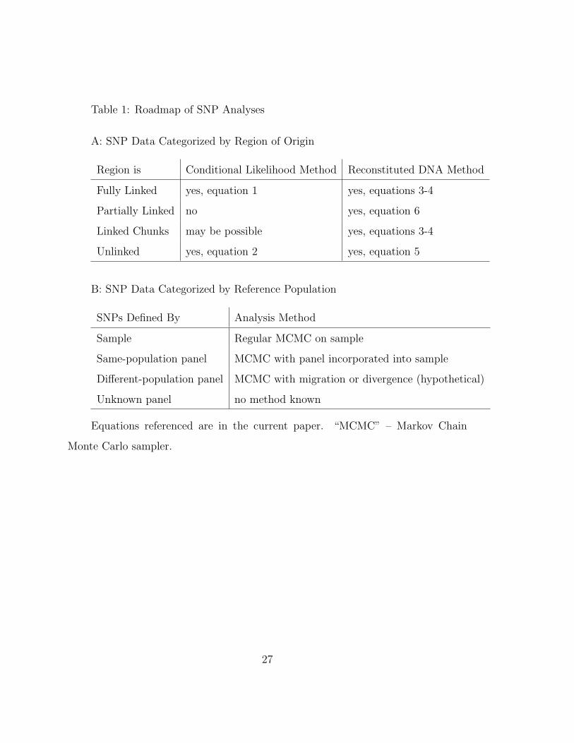
Table 1: Roadmap of SNP Analyses
A: SNP Data Categorized by Region of Origin
Region is Conditional Likelihood Method Reconstituted DNA Method
Fully Linked yes, equation 1 yes, equations 3-4
Partially Linked no yes, equation 6
Linked Chunks may be possible yes, equations 3-4
Unlinked yes, equation 2 yes, equation 5
B: SNP Data Categorized by Reference Population
SNPs Defined By Analysis Method
Sample Regular MCMC on sample
Same-population panel MCMC with panel incorporated into sample
Different-population panel MCMC with migration or divergence (hypothetical)
Unknown panel no method known
Equations referenced are in the current paper. “MCMC” – Markov Chain
Monte Carlo sampler.
27
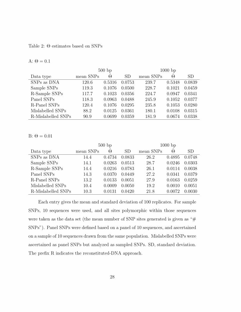
Table 2: Θ estimates based on SNPs
A: Θ = 0.1
500 bp 1000 bp
Data type mean SNPs Θ SD mean SNPs Θ SDSNPs as DNA 120.6 0.5316 0.0753 239.7 0.5348 0.0839Sample SNPs 119.3 0.1076 0.0500 228.7 0.1021 0.0459R-Sample SNPs 117.7 0.1023 0.0356 224.7 0.0947 0.0341Panel SNPs 118.3 0.0963 0.0488 245.9 0.1052 0.0377R-Panel SNPs 120.4 0.1076 0.0295 235.8 0.1053 0.0280Mislabelled SNPs 88.2 0.0125 0.0361 180.1 0.0108 0.0315R-Mislabelled SNPs 90.9 0.0699 0.0359 181.9 0.0674 0.0338
B: Θ = 0.01
500 bp 1000 bp
Data type mean SNPs Θ SD mean SNPs Θ SDSNPs as DNA 14.4 0.4734 0.0833 26.2 0.4895 0.0748Sample SNPs 14.1 0.0263 0.0513 28.7 0.0246 0.0303R-Sample SNPs 14.4 0.0216 0.0783 26.1 0.0114 0.0038Panel SNPs 14.3 0.0370 0.0449 27.2 0.0341 0.0379R-Panel SNPs 13.2 0.0133 0.0051 27.9 0.0163 0.0259Mislabelled SNPs 10.4 0.0009 0.0050 19.2 0.0010 0.0051R-Mislabelled SNPs 10.3 0.0131 0.0420 21.8 0.0072 0.0030
Each entry gives the mean and standard deviation of 100 replicates. For sample
SNPs, 10 sequences were used, and all sites polymorphic within those sequences
were taken as the data set (the mean number of SNP sites generated is given as “#
SNPs”). Panel SNPs were defined based on a panel of 10 sequences, and ascertained
on a sample of 10 sequences drawn from the same population. Mislabelled SNPs were
ascertained as panel SNPs but analyzed as sampled SNPs. SD, standard deviation.
The prefix R indicates the reconstituted-DNA approach.
28
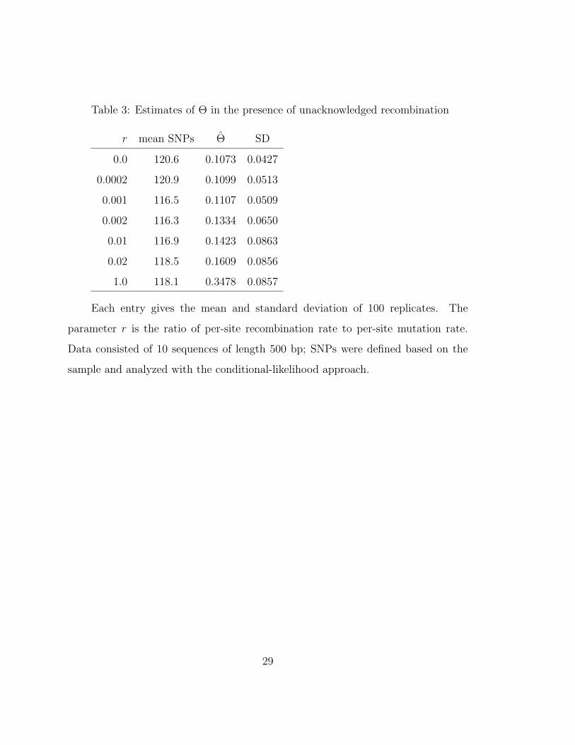
Table 3: Estimates of Θ in the presence of unacknowledged recombination
r mean SNPs Θ SD
0.0 120.6 0.1073 0.0427
0.0002 120.9 0.1099 0.0513
0.001 116.5 0.1107 0.0509
0.002 116.3 0.1334 0.0650
0.01 116.9 0.1423 0.0863
0.02 118.5 0.1609 0.0856
1.0 118.1 0.3478 0.0857
Each entry gives the mean and standard deviation of 100 replicates. The
parameter r is the ratio of per-site recombination rate to per-site mutation rate.
Data consisted of 10 sequences of length 500 bp; SNPs were defined based on the
sample and analyzed with the conditional-likelihood approach.
29
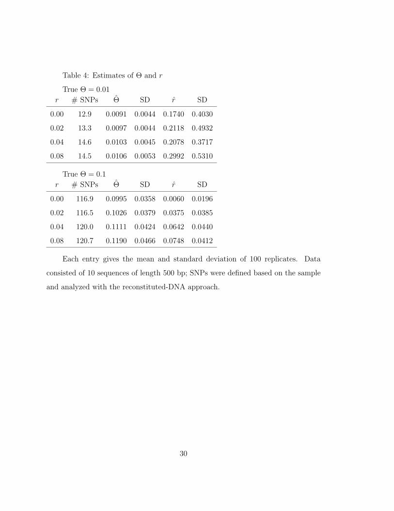
Table 4: Estimates of Θ and r
True Θ = 0.01
r # SNPs Θ SD r SD
0.00 12.9 0.0091 0.0044 0.1740 0.4030
0.02 13.3 0.0097 0.0044 0.2118 0.4932
0.04 14.6 0.0103 0.0045 0.2078 0.3717
0.08 14.5 0.0106 0.0053 0.2992 0.5310
True Θ = 0.1
r # SNPs Θ SD r SD
0.00 116.9 0.0995 0.0358 0.0060 0.0196
0.02 116.5 0.1026 0.0379 0.0375 0.0385
0.04 120.0 0.1111 0.0424 0.0642 0.0440
0.08 120.7 0.1190 0.0466 0.0748 0.0412
Each entry gives the mean and standard deviation of 100 replicates. Data
consisted of 10 sequences of length 500 bp; SNPs were defined based on the sample
and analyzed with the reconstituted-DNA approach.
30
Recommended