Transport in Porous Media manuscript No.(will be inserted by the editor)
Upscaling non-Darcy flow
C.R. Garibotti · M.Peszynska
Received: date / Accepted: date
Abstract We consider upscaling of non-Darcy flow in heterogeneous porous media.
Our approach extends the pressure-based numerical homogenization procedure for lin-
ear Darcy flow, due to Durlofsky, to the nonlinear case. The effective coefficients are
not constants but rather mildly varying functions of prevailing gradients of pressure.
The upscaled model approximates the fine grid model accurately and, in some cases,
more accurately than what is expected for Darcy flow; this is due to the non–Darcy ef-
fects which suppress heterogeneity. We provide comparisons of alternative approaches
as well as consider several variants of numerical realizations of the non–Darcy flow
model. Numerical results show effectiveness of the upscaling procedure.
Keywords non-Darcy flow · upscaling · numerical homogenization · finite differences ·mixed finite elements
Mathematics Subject Classification (2000) 76S05 · 65N06 · 76M50 · 65N30 ·35B27
1 Introduction
When modeling flow and transport in heterogeneous porous media using numerical
methods one often needs to consider a scale H coarser than the h scale at which the
data are given. Over the last two or three decades various techniques of upscaling from
scale h to H, also called numerical homogenization, have been defined and critically
evaluated, see original papers [14], review [45], and recent work [49,28,8,7]. While
methods of upscaling for linear single equation models are reasonably well understood,
upscaling nonlinear models or systems, beyond the progress made for multiphase flow
[1,17,7], remains, in general, an open field.
Partially supported by National Science Foundation grant 0511190 and Department of Energygrant 98089. Corresponding author: M. Peszynska.
C. Garibotti E-mail: [email protected]. Peszynska E-mail: [email protected] Department, Oregon State University, Corvallis, OR 97331Tel.: +1-541-737-9847, Fax: +1-541-737-0517
2
In this paper we are concerned with upscaling of non-Darcy model of single-phase
incompressible fluid flow in saturated porous medium Ω ⊂ IRd, d = 1, 2, 3, in the form
(K−1 + βI|u|)u = −∇p. (1)
This extends the linear Darcy’s law
u = −K∇p, (2)
with p denoting pressure or potential, K denoting the hydraulic conductivity tensor,
I ∈ IRd×d the identity matrix and where u is the velocity (volumetric flux) of the
fluid. Here β is the nonnegative scalar known as the Forchheimer coefficient, and the
model (1) is due to Forchheimer [25]. Clearly if β = 0, then (1) reduces to (2). Other
formulations are available in literature; we develop these and the notation in Section 2.
The conservation of mass is given by
∇ · u = 0, (3)
or, more generally, with a distributed source q by
∇ · u = q. (4)
The central issue addressed in this paper concerns heterogeneous porous media
when K = K(x),x ∈ Ω. We assume β ≡ const or β = β(x) which occurs for example
when β is correlated to K via some relationship β = g(K).
Specifically, the natural question that arises is how to upscale the model (1), (3).
That is, given values of Kh and βh at a scale h, what values of KH and βH should
one use in a numerical model at a scale H >> h ? In particular, if βh is constant, is
it appropriate to assume so for βH ? Similar questions arise when βh is not constant
but rather correlated to Kh; the answers are not straightforward due to nonlinearity
of (1).
For the linear case, that is, Darcy’s flow (2)–(3), various upscaling and numerical
homogenization methods have been shown to be very effective; see [14,45,8,28]. Com-
bine (2) and (3) and consider a numerical approximation on grid parametrized by h of
the resulting elliptic PDE, −∇h · (Kh∇hph) = 0. Upscaling to scale H means we want
to solve −∇H · (KH∇HpH) = 0, where the upscaled coefficient KH is obtained from
one of the known methods; see details in Section 4.
Upscaling of nonlinear models presents a challenge. In particular, consider a non-
linear PDE of the form
∇ · K(∇ph) = 0,
where K(ξh) = K(θh; ξh) is a general nonlinear function of ξ parameterized by some pa-
rameters θ, both given at scale h. In general, there is no guarantee that the nonlinearity
K∗ in the upscaled model
∇ · K∗(∇pH) = 0,
is parameterized in the same way as K is in the original model, and even if so, that
these parameters are equal to some upscaled θH . In other words, in general it is not
true that one has K∗(ξH) = K(θH ; ξH). Rather, to identify K∗, one has to consider a
collection of nonlinear upscaled maps; these follow from solutions to local cell problems
3
Fig. 1 Schematic difference between linear and nonlinear upscaling. Left: linear upscaling ofKh delivers a constant upscaled value KH . Right: nonlinear upscaling of βh delivers a mapβH(α) where α represents a local boundary condition value.
posed at the scale h with cells of size H but in general are not decoupled from the
global equation; see [16,7,18]. Additional difficulties in using θH arise for systems even
if they are linear [40]. See Figure 1 for illustration.
In the problem of interest to this paper, in the nonlinear PDE obtained from (1),
(3), we have K(ξh) = K(Kh, βh; ξh). In what follows we show that upscaling of K gives
a satisfactory upscaled model with K∗(ξH) = K(KH , βH ; ξH), where the upscaled
coefficients KH , βH are computed numerically via solutions to cell problems. It turns
out that βH is, in general, not constant but varies midlly with the average flow rates.
We focus primarily on pressure-based upscaling after Durlofsky [14].
As a result, we obtain an efficient and accurate method of upscaling (1). We believe
that the success of this nonlinear upscaling procedure is due to the fact that the inertia
effects appear to supress heterogeneity of K for large β, which of course helps in the
process of upscaling. In addition, we show that in some cases it is reasonable to use
a simpler upscaled model with K∗(ξH) ≈ K(KH , βgH ; ξH) where βg
H does not require
nonlinear upscaling.
Nonlinear upscaling methods with applications to porous media have been applied
to multiphase flow problems. There, in addition to deriving KH , one considers up-
scaling of nonlinear multiphase flow properties such as saturation-dependent relative
permeabilities and/or capillary pressure relationships. The use of pseudo-functions [3,
10] is considered an effective yet not always fully satisfactory approach. Difficulty in
upscaling multiphase models is associated with large heterogeneity contrasts, with de-
pendence of multiphase flow properties on rock-type, as well as with the nonlinear
coupled nature of systems of PDEs that have to be solved. For ongoing research see [8,
7].
On the other hand, there has been considerable research devoted to analysis [24]
and numerical approximation [12,36] of non-Darcy flow in homogeneous porous me-
dia. To our knowledge, however, not much work has been done for non-Darcy flow in
heterogeneous media or devoted to the effects the Forchheimer correction has on the
flow in heterogeneous case. In non-Darcy case, the only considerations known to us
are in [35] where a scalar case is considered and recent work in [34] where a separate
approach applicable to fractured media is considered. In this paper we take a first step
towards upscaling of non-Darcy flow for flow driven by boundary conditions only. When
q 6≡ 0, for example, when wells are present, non-Darcy flow in homogeneous media was
considered in [22]; upscaling around wells for Darcy or for multiphase flow has been
considered in [48,11]. Upscaling of non-Darcy flow around wells is outside the present
scope.
4
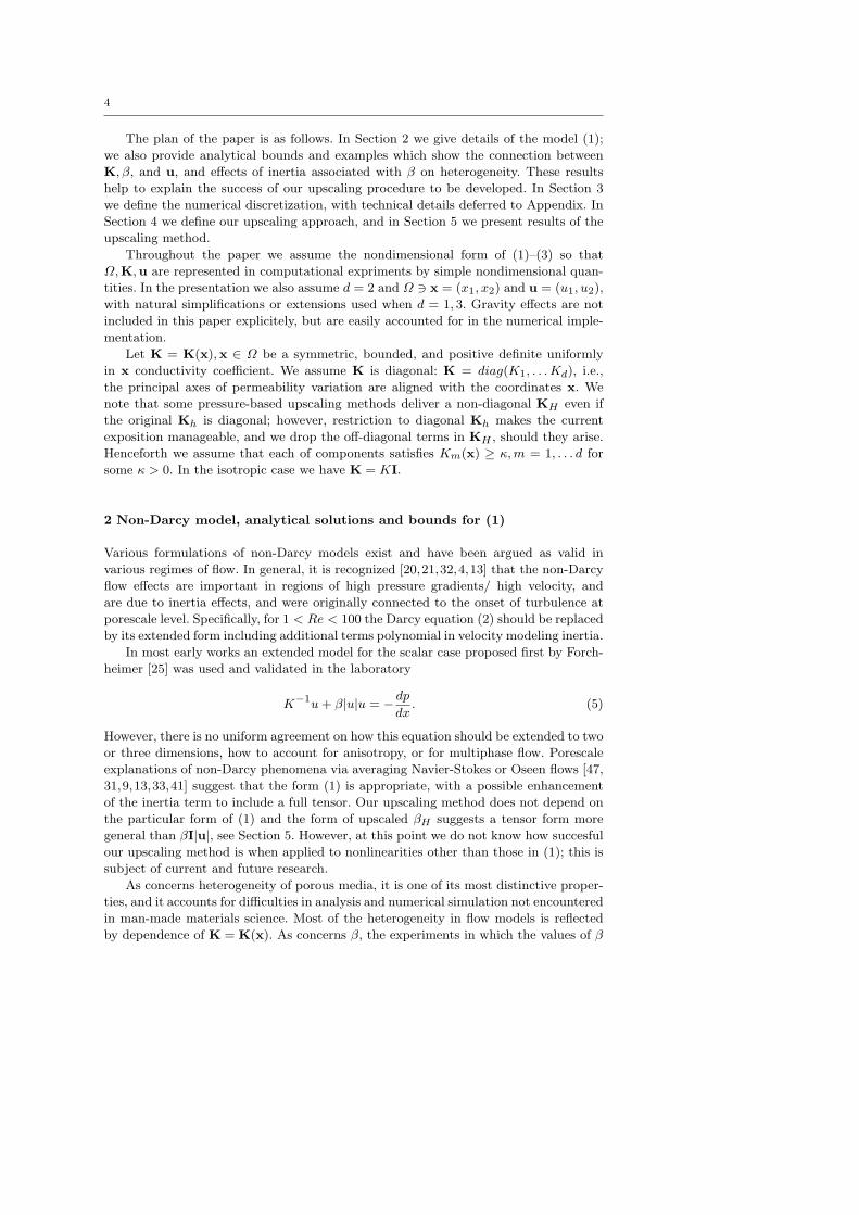
The plan of the paper is as follows. In Section 2 we give details of the model (1);
we also provide analytical bounds and examples which show the connection between
K, β, and u, and effects of inertia associated with β on heterogeneity. These results
help to explain the success of our upscaling procedure to be developed. In Section 3
we define the numerical discretization, with technical details deferred to Appendix. In
Section 4 we define our upscaling approach, and in Section 5 we present results of the
upscaling method.
Throughout the paper we assume the nondimensional form of (1)–(3) so that
Ω,K,u are represented in computational expriments by simple nondimensional quan-
tities. In the presentation we also assume d = 2 and Ω ∋ x = (x1, x2) and u = (u1, u2),
with natural simplifications or extensions used when d = 1, 3. Gravity effects are not
included in this paper explicitely, but are easily accounted for in the numerical imple-
mentation.
Let K = K(x),x ∈ Ω be a symmetric, bounded, and positive definite uniformly
in x conductivity coefficient. We assume K is diagonal: K = diag(K1, . . .Kd), i.e.,
the principal axes of permeability variation are aligned with the coordinates x. We
note that some pressure-based upscaling methods deliver a non-diagonal KH even if
the original Kh is diagonal; however, restriction to diagonal Kh makes the current
exposition manageable, and we drop the off-diagonal terms in KH , should they arise.
Henceforth we assume that each of components satisfies Km(x) ≥ κ,m = 1, . . . d for
some κ > 0. In the isotropic case we have K = KI.
2 Non-Darcy model, analytical solutions and bounds for (1)
Various formulations of non-Darcy models exist and have been argued as valid in
various regimes of flow. In general, it is recognized [20,21,32,4,13] that the non-Darcy
flow effects are important in regions of high pressure gradients/ high velocity, and
are due to inertia effects, and were originally connected to the onset of turbulence at
porescale level. Specifically, for 1 < Re < 100 the Darcy equation (2) should be replaced
by its extended form including additional terms polynomial in velocity modeling inertia.
In most early works an extended model for the scalar case proposed first by Forch-
heimer [25] was used and validated in the laboratory
K−1u+ β|u|u = − dp
dx. (5)
However, there is no uniform agreement on how this equation should be extended to two
or three dimensions, how to account for anisotropy, or for multiphase flow. Porescale
explanations of non-Darcy phenomena via averaging Navier-Stokes or Oseen flows [47,
31,9,13,33,41] suggest that the form (1) is appropriate, with a possible enhancement
of the inertia term to include a full tensor. Our upscaling method does not depend on
the particular form of (1) and the form of upscaled βH suggests a tensor form more
general than βI|u|, see Section 5. However, at this point we do not know how succesful
our upscaling method is when applied to nonlinearities other than those in (1); this is
subject of current and future research.
As concerns heterogeneity of porous media, it is one of its most distinctive proper-
ties, and it accounts for difficulties in analysis and numerical simulation not encountered
in man-made materials science. Most of the heterogeneity in flow models is reflected
by dependence of K = K(x). As concerns β, the experiments in which the values of β
5
were calculated for a given isotropic rock sample suggest that β may be correlated with
various powers of K [27]. Also, β is high for carbonate rocks such as limestone and
sandstone and generally higher for vugular than for non-vugular rocks [30]. In general,
it is reasonable to conclude that in heterogeneous nonisotropic porous media, β = β(x)
whenever K = K(x).
In this paper we report, for simplicity, only on two variants of β, indexed by B,
which for isotropic K = KI read
β = gB(β0,K) =
β0, B = 0β0√K, B = 1
. (6)
More [27,30] can be easily incorporated. However, a special case of non-smooth g
such as the one for fracture systems where inertia terms are neglected in the matrix,
will not be considered here but is a topic of future work. See also Section 5.3.4 on
our computational results regarding correlation. In general β may actually vary with
pressure and/or composition of fluids, and some formulations of (1) account for this
[12,23,24,22]. For simplicity throughout this paper we consider a fixed single phase
fluid and, hence, we lump the viscosity and density coefficients along with K, β.
For nonisotropic diagonal K the correlations (6) should be considered component-
wise; we find it therefore natural to allow for β = (β1, β2) to be a vector. Non-isotropic
β may also arise in the process of upscaling; a vector form of β does not introduce
additional difficulties in a numerical model. With this, we rewrite (1) componentwise,
with the coupling term between components given by |u| =
√
∑dm=1 u
2m,
(K−1m + βm|u|)um = − ∂p
∂xm, m = 1, . . . d. (7)
A simplified version, in which the nonlinearity in velocity components is decoupled, is
the one adapted in [22], and it is a multi-dimensional analogue of (5),
(K−1m + βm|um|)um = − ∂p
∂xm, m = 1, . . . d. (8)
Since (7) is more general, it will be used as a basis for numerical models. Interestingly,
in some numerical discretizations, a discrete version of (8) arises on its own from
discretization of (7).
2.1 Analytical solution and bounds
It is not difficult to find an analytical solution u to (5). In the multidimensional case, it
may no more be directly possible. Below we derive bounds which are helpful in scalar
and non-scalar cases.
2.1.1 Estimates for scalar case
Let D = − dpdx . Rewrite (5) as
u = K(D), (9)
6
D
u(1
,0;D
),u(
1,1e
-4;D
),u(
1,1
e-2;
D)
0 200 400 600 800 10000
200
400
600
800
1000 u(1,0;D)u(1,1e-4;D)u(1,1e-2;D)
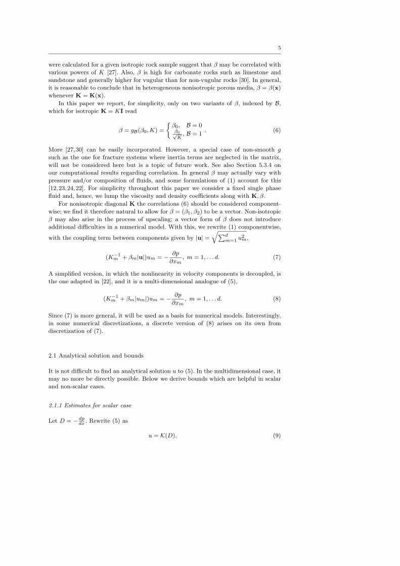
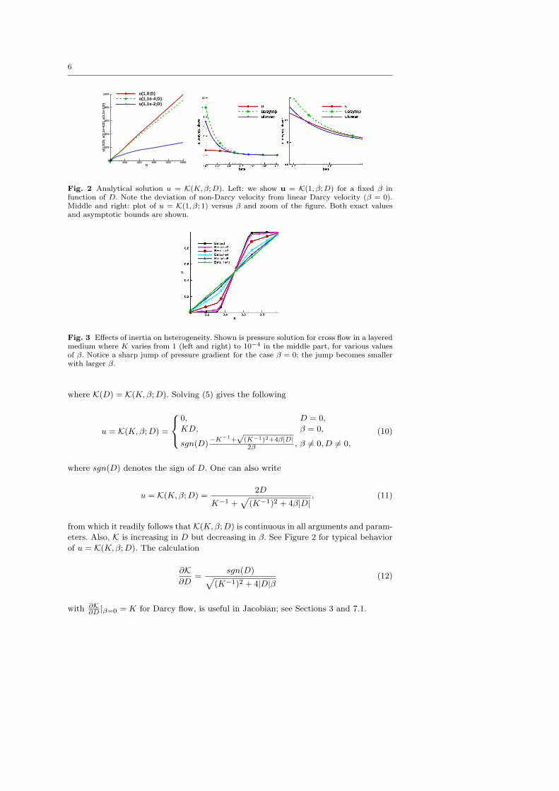
Fig. 2 Analytical solution u = K(K, β; D). Left: we show u = K(1, β; D) for a fixed β infunction of D. Note the deviation of non-Darcy velocity from linear Darcy velocity (β = 0).Middle and right: plot of u = K(1, β; 1) versus β and zoom of the figure. Both exact valuesand asymptotic bounds are shown.
Fig. 3 Effects of inertia on heterogeneity. Shown is pressure solution for cross flow in a layeredmedium where K varies from 1 (left and right) to 10−4 in the middle part, for various valuesof β. Notice a sharp jump of pressure gradient for the case β = 0; the jump becomes smallerwith larger β.
where K(D) = K(K,β;D). Solving (5) gives the following
u = K(K,β;D) =
0, D = 0,
KD, β = 0,
sgn(D)−K−1+
√(K−1)2+4β|D|2β , β 6= 0, D 6= 0,
(10)
where sgn(D) denotes the sign of D. One can also write
u = K(K,β;D) =2D
K−1 +√
(K−1)2 + 4β|D|, (11)
from which it readily follows that K(K,β;D) is continuous in all arguments and param-
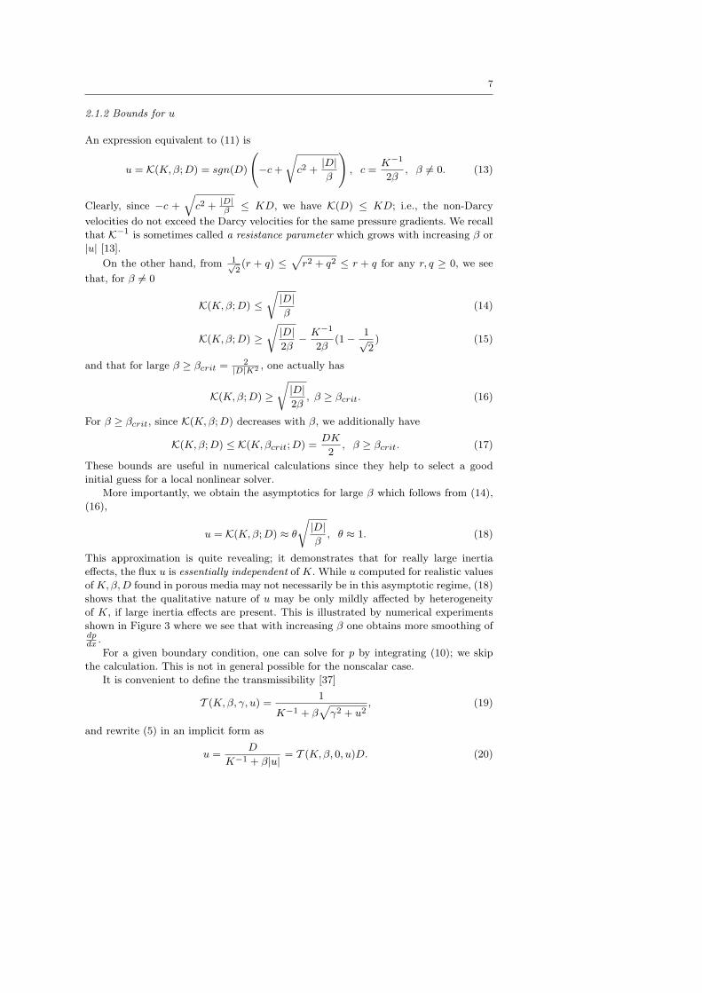
eters. Also, K is increasing in D but decreasing in β. See Figure 2 for typical behavior
of u = K(K,β;D). The calculation
∂K∂D
=sgn(D)
√
(K−1)2 + 4|D|β(12)
with ∂K∂D |β=0 = K for Darcy flow, is useful in Jacobian; see Sections 3 and 7.1.
7
2.1.2 Bounds for u
An expression equivalent to (11) is
u = K(K,β;D) = sgn(D)
(
−c+
√
c2 +|D|β
)
, c =K−1
2β, β 6= 0. (13)
Clearly, since −c +
√
c2 +|D|β ≤ KD, we have K(D) ≤ KD; i.e., the non-Darcy
velocities do not exceed the Darcy velocities for the same pressure gradients. We recall
that K−1 is sometimes called a resistance parameter which grows with increasing β or
|u| [13].
On the other hand, from 1√2(r + q) ≤
√
r2 + q2 ≤ r + q for any r, q ≥ 0, we see
that, for β 6= 0
K(K,β;D) ≤√
|D|β
(14)
K(K,β;D) ≥√
|D|2β
− K−1
2β(1 − 1√
2) (15)
and that for large β ≥ βcrit = 2|D|K2 , one actually has
K(K,β;D) ≥√
|D|2β
, β ≥ βcrit. (16)
For β ≥ βcrit, since K(K,β;D) decreases with β, we additionally have
K(K,β;D) ≤ K(K,βcrit;D) =DK
2, β ≥ βcrit. (17)
These bounds are useful in numerical calculations since they help to select a good
initial guess for a local nonlinear solver.
More importantly, we obtain the asymptotics for large β which follows from (14),
(16),
u = K(K,β;D) ≈ θ
√
|D|β, θ ≈ 1. (18)
This approximation is quite revealing; it demonstrates that for really large inertia
effects, the flux u is essentially independent of K. While u computed for realistic values
of K,β,D found in porous media may not necessarily be in this asymptotic regime, (18)
shows that the qualitative nature of u may be only mildly affected by heterogeneity
of K, if large inertia effects are present. This is illustrated by numerical experiments
shown in Figure 3 where we see that with increasing β one obtains more smoothing ofdpdx .
For a given boundary condition, one can solve for p by integrating (10); we skip
the calculation. This is not in general possible for the nonscalar case.
It is convenient to define the transmissibility [37]
T (K,β, γ, u) =1
K−1 + β√
γ2 + u2, (19)
and rewrite (5) in an implicit form as
u =D
K−1 + β|u| = T (K,β, 0, u)D. (20)
8
2.1.3 Non-scalar case
Now we set Dm = − ∂p∂xm
, and use γ2 =∑
n6=m(un)2 which combines all components
of velocity other than m, and we rewrite (7)
(
K−1m + βm
√
γ2 + (um)2)
um = Dm. (21)
We then have
um = T
Km, βm,
√
∑
n6=2
u2n, um
Dm.
Note that T (Km, βm,
√
∑
n6=2 u2n, um) = T (Km, βm, 0, |u|); this simplifies the forth-
coming numerical calculations discussed in Section 7.1.
Given (un)n6=m, that is, γ, one can find um explicitly from (21) and/or derive
estimates similar to those for the scalar case. In general of course, γ itself is unknown.
However, given Dm,m = 1, . . . d, one can solve (21) by fixed point or Newtonian
iteration. Difficulties arise in numerical calculations because the discrete form of (21)
involves a large stencil; see Sections 3 and 7.2.
3 Numerical discretization
Here we formulate a discrete version of (3) and (1) as a cell-centered finite difference
method (CCFD) in several variants depending on discretization of |u| in (7). These
variants and discretization are motivated using mixed Finite Elements in Section 7.2;
this development has a theoretical value in that the convergence results proved in
[36] for mixed FE methods apply to our discretization. Additionally, we obtain insight
into why a particular discrete version of (7) is justified. From the point of view of
upscaling, we show later that all the variants behave similarly; in other words, the
success of upscaling is not tied to a particular variant of discretization.
Let the region Ω be decomposed into rectangular elements or cells Ωij on a Carte-
sian grid with natural notation of xij = (x1,ij , x2,ij) denoting cell centers. The ele-
ments Ωij are of size xi × yj . The edge Ei+1/2,j between Ωij and Ωi+1,j has a
center at (x1,i+1/2,j , yj), and so on. The distances between cell centers are denoted
by xi+1/2,j etc.. The parameter h is the maximum of either xi,yj . When coarse
grid with parameter H is used, we index the cells using I, J .
The discrete pressures ph ≡ (pij)i,j=1 are associated with cell centers. The normal
components of velocities are associated with midpoints of cell edges; on the cell Ωij the
velocity in direction x1 is defined by its values u1,i−1/2,j on the left and u1,i+1/2,j on
the right edges. The discrete velocities uh can be then considered to be a tensor product
of piecewise linear polynomials in x1 direction and piecewise constant polynomials in
the x1 direction and opposite in the x2 direction. The notation is standard; see [37,46,
6] for details.
Recall [37,46] the standard discrete counterpart of (3)
∇h · uh = 0, (22)
9
and of (2), which we develop now. In the direction x1 we have
u1,i+1/2,j = K1,i+1/2,jpi,j − pi+1,j
xi+1/2,j= T1,i+1/2,j
(
pi,j − pi+1,j
)
, (23)
where transmissibility T1,i+1/2,j =K1,i+1/2,j
xi+1/2,jis defined, and harmonic averaging of
permabilities is used [37]:
K−11,i+1/2,j =
1
2 xi+1/2,j
(
K−11,ij xi +K
−11,i+1,j xi+1
)
. (24)
3.1 Discrete non-Darcy velocities
With notation as above, we can now state the following discrete counterpart of (1) or
(7), with mixed finite element derivation deferred to Section 7.2:
(
T−11,i+1,j +
1
2
(
β1,ij xi|uh|+i,j + β1,i+1,j xi+1|uh|−i+1,j
)
)
u1,i+1/2,j
= pi,j − pi+1,j . (25)
An analogous definition can be written immediately in direction x2.
The crucial point is to define the terms |uh|+i,j and |uh|−i+1,j . These have the mean-
ing of magnitude of velocity on the cells i, j and i+ 1, j, respectively, each relative to
the edge Ei+1/2,j on which the velocity component u1,i+1/2,j is being defined. They
can be defined in several ways, which we denote below as variants V = 0, 1, 2, 3.
Consider |uh|+i,j , with |uh|−i,j defined analogously. The simplest way to define it
(V = 0) is to use the magnitude of normal component of uh on the edge Ei+1/2,j that
is, |u1,i+1/2,j |, as was done in [22].
Another way, V = 2, is to use the magnitude of uh itself on the edge Ei+1/2,j
which is defined using
(uh)+ij =
(
u1,i+1/2,j ,u2,i,j+1/2 + u2,i,j−1/2
2
)
(uh)−ij =
(
u1,i+1/2,j ,u2,i+1,j+1/2 + u2,i+1,j−1/2
2
)
,
or, with the quantity (V = 1),
(uh)ij =(uh)+ij + (uh)−ij
2.
Finally, the most general way, called V = 3, is to use the magnitude(s) of (interpolated)
value(s) of
(uh)ij =
(
u1,i+1/2,j + u1,i−1/2,j
2,u2,i,j+1/2 + u2,i,j−1/2
2
)
,
(uh)i+1,j =
(
u1,i+1/2,j + u1,i+3/2,j
2,u2,i+1,j+1/2 + u2,i+1,j−1/2
2
)
,
in the middle of cells Ωij and Ωi+1,j , respectively.
10
Summarizing, we define
|uh|+i,j =
|u1,i+1/2,j |, variant = 0,
|(uh)ij |, variant = 1,
|(uh)+ij |, variant = 2,
|(uh)ij |, variant = 3.
(26)
These four variants lead to somewhat different numerical solutions to (1)-(3).
Variant V = 0 is a direct discretization of (8); it can also be seen as a simplifica-
tion/approximation of variants V = 1, 2. It uses the same 5-point stencil as used for
Darcy’ law with diagonal K and allows for analytical component-wise resolution of
local nonlinearities.
Variants V = 1, 2, 3 are associated each with a different method of numerical inte-
gration in mixed FE applied to (7); see Section 7.2. The difference between V = 1 and
V = 2 is not larger than the one appearing in the use of numerical quadrature to derive
(23) from (2) using mixed FE. Both variants couple the velocity u1,i+1/2,j to four other
velocity degrees of freedom, and are equivalent to each other up to higher order terms;
see Section 7.2. With V = 1 we have symmetry in that |uh|+i,j = |uh|−i+1,j , and one
can get around the difficulty of an enlarged stencil when resolving local nonlinearities,
by iteration-lagging those components in |(uh)ij | other than u1,i+1/2,j . Variant V = 2
is somewhat more complicated than V = 1, because |uh|+i,j is not identical to |uh|−i,j .Variant V = 3 is the most complex one, and, if applied in (25) alone, it couples
velocity u1,i+1/2,j and pressures pi,j , pi+1,j to 6 other velocity degrees of freedom
appearing in its definition and thereby to 6 additional pressure values. The stencil in
the resulting discrete system is increased from 5-point to 13-point in d = 2. In addition,
resolution of local nonlinearity is not very succesful by iteration lagging and impossible
directly. While we performed numerical experiments with this variant, its complexity
is not offering promise of being a succesful model.
In view of the above, only V = 0, 1 will be discussed further. In summary then,
discretization of (7) or (8) takes the form
(
T−11,i+1,j +B1,i+1/2,j |(uh)Vi+1/2,j |
)
u1,i+1/2,j = pi,j − pi+1,j , (27)
where we define B1,i+1/2,j = 12
(
β1,ij xi + β1,i+1,j xi+1
)
= xi+1/2β1,i+1/2,j ,
and where |(uh)Vi+1/2,j | is computed according to (26).
It is convenient to cast (27) in a form similar to (23) and (20). Define the trans-
missibilities ΥV1,i+1/2,j which, unlike T1,i+1/2,j , depend nonlinearly on the solution,
ΥV1,i+1/2,j = T (T1,i+1/2,j , B1,i+1/2,j , 0, |(uh)Vi+1/2,j |), (28)
with a similar definition for Υ2,i,j+1/2. Now (27) reads, for every i, j
u1,i+1/2,j = ΥV1,i+1/2,j(pi,j − pi+1,j), (29)
u2,i,j+1/2 = ΥV2,i,j+1/2(pi,j − pi,j+1), (30)
and in a vector form we can write symbolically, for uh =(
(u1,i+1/2,j , u2,i,j+1/2))
ij,
uh = TV (Kh, βh, |uh|,uh)∇hph = TVh∇hph. (31)
11
Note finally that if β ≡ 0 we have TV (Kh, 0, |uh|,uh) ≡ −Kh. Also, recall that if
V = 0, the implicit relationships (29) and (30) can be resolved explicitely.
This formulation is used in the remainder of this paper; see Section 7.2 for mixed
FE derivation and Section 7.1 for details of nonlinear solver. Also, see Section 5 for
discussion of the difference between variants V = 0, 1. To complete this Section, we
comment on boundary conditions.
3.1.1 Boundary conditions
D
N
D
N
D
D
N N
D
N
D
N
N
N
P
P
P P+jump
B1 B2 B3 BP
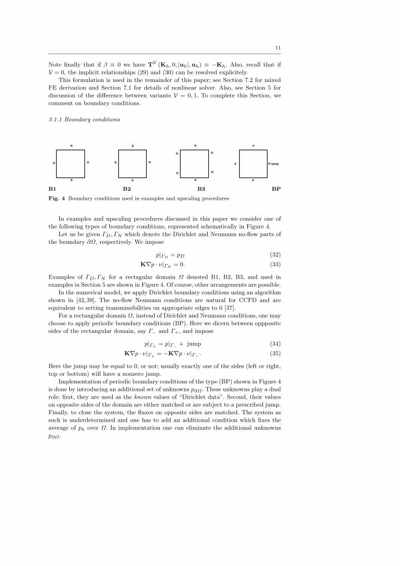
Fig. 4 Boundary conditions used in examples and upscaling procedures
In examples and upscaling procedures discussed in this paper we consider one of
the following types of boundary conditions, represented schematically in Figure 4.
Let us be given ΓD, ΓN which denote the Dirichlet and Neumann no-flow parts of
the boundary ∂Ω, respectively. We impose
p|ΓD= pD (32)
K∇p · ν|ΓN= 0. (33)
Examples of ΓD, ΓN for a rectagular domain Ω denoted B1, B2, B3, and used in
examples in Section 5 are shown in Figure 4. Of course, other arrangements are possible.
In the numerical model, we apply Dirichlet boundary conditions using an algorithm
shown in [42,39]. The no-flow Neumann conditions are natural for CCFD and are
equivalent to setting transmissibilities on appropriate edges to 0 [37].
For a rectangular domain Ω, instead of Dirichlet and Neumann conditions, one may
choose to apply periodic boundary conditions (BP). Here we dicern between oppposite
sides of the rectangular domain, say Γ− and Γ+, and impose
p|Γ+= p|Γ−
+ jump (34)
K∇p · ν|Γ+= −K∇p · ν|Γ−
. (35)
Here the jump may be equal to 0, or not; usually exactly one of the sides (left or right,
top or bottom) will have a nonzero jump.
Implementation of periodic boundary conditions of the type (BP) shown in Figure 4
is done by introducing an additional set of unknowns p∂Ω . These unknowns play a dual
role: first, they are used as the known values of “Dirichlet data”. Second, their values
on opposite sides of the domain are either matched or are subject to a prescribed jump.
Finally, to close the system, the fluxes on opposite sides are matched. The system as
such is underdetermined and one has to add an additional condition which fixes the
average of ph over Ω. In implementation one can eliminate the additional unknowns
p∂Ω .

12
4 Upscaling
This section provides answers to the core issues addressed in this paper. Let us be given
a scale h, identified as diameter of Ωij , on which the coefficients Kh, βh are given, but
at which it is practically impossible to solve the system (53). Assume there is a coarse
scale H >> h at which such computations are possible. The main issue is to find the
equations which describe the problem at scale H, and to identify their coefficients. Our
premise is that this is possible and that an upscaled version of (53)
∇H · TVH∇HpH = 0 (36)
can be identified.
Alternatively, one can use a numerical method at scale H which incorporates the
variation of Kh in its definition; this is done in subgrid upscaling or multiscale and vari-
ational approaches to Finite Element methods; see [2,19,15,18,17] and related work.
Yet another alternative is to use mortar upscaling [42].
Our approach in this paper in using (36) is traditional, and we aim to derive KH , βH
from Kh, βh. We briefly review what was done for Darcy flow and then proceed to non-
Darcy case.
4.1 Upscaling Kh and notation
For Darcy flow it is standard to consider the upscaled linear system at scale H to be
of the same form as the one at h, which is also linear. Various methods M of upscaling
(K)h 7→ (K)H have been reviewed in [45]; these include arithmetic M = A or harmonic
M = H averaging and give (K)AH , (K)HH , respectively. The pressure-based methods
[14] which deliver (K)DH ,(K)PH and use Dirichlet and periodic boundary conditions,
respectively, perform better than M = A,H but are more computationally expensive.
They are related to homogenization methods pursued in mathematical analysis [5].
Here we briefly recall the method proposed in [14]. Fix a grid cell ΩIJ at scale H.
By upscaling Darcy flow coefficients, we want to ensure that (23) holds on the grid
H. Since (23) is linear, it is natural to ask that the fluxes on grid H which arise due
to pressure gradients imposed on that grid, agree on average with fluxes on grid h,
when these arise from the same global pressure gradients; this requirement preserves
mass. With this approach, one finds KH |ΩIJby inverse modeling as the appropriate
coefficient of proportionality. The caveat is that one has to solve a cell problem on
ΩIJ subject to some global pressure gradients in order to compute that response. How
these pressure gradients are imposed determines the D and P methods.
Consider first the local cell problem with Dirichlet boundary conditions of type B1,
see Figure 4. We solve for ph, uh
−∇h · (Kh∇hph) = 0, y ∈ ΩIJ (37)
p|Γ1,I−1/2,J= 0 (38)
p|Γ1,I+1/2,J= DI,J (39)
(Kh∇p · n)|Γ2,I,J+1/2∪Γ2,I,J−1/2= 0. (40)
13
Then we compute the total flux u1,I+1/2,J =∫
Γ1,I,J+1/2uh ·n, and we find KD
1,I+1/2,J
by fitting it into the counterpart of (23)
u1,I+1/2,J = KD1,I,J
DI,J
xI,J. (41)
Next, we solve an analogous cell problem with boundary conditions B2 to find KD2,I,J .
The two values KD1,I,J ,K
D2,I,J form the diagonal upscaled tensor KD
I,J . Repeating cell
calculations on all cells I, J of the grid at scale H, we obtain the collection of diagonal
conductivities KH ≡(
KDI,J
)
IJ.
Instead of using Dirichlet boundary conditions B1, B2, one can solve (37)–(40)
subject to periodic boundary conditions (34), (35), see BP in Figure 4. The jump is
now DIJ . However, the coefficients (KH)PIJ that one gets from inverse matching of
fluxes across all boundaries are, in general, not diagonal even if Kh is diagonal.
The global system −∇H · (KH∇HpH) = 0 solved for pH on grid H with (K)MHfor M = D,P , has reasonable accuracy of global flow patterns in the sense that they
resemble closely those for grid h. In general, M = P leads to better accuracy of global
flow patterns than M = D does, and both are more accurate than M = A,H. See
further discussion of metrics of upscaling accuracy in Section 5.
4.2 Upscaling non-Darcy flow with a pressure-based method
For non-Darcy flow, the underlying problem at scale h is nonlinear and therefore it is
not straighforward to see whether the problem at scale H has the same structure as
the one at scale h, and even if so, how to obtain Kh 7→ KH , and βh 7→ βH .
The following idea comes to mind. Let us be given Kh, βh and some scale H >> h.
LetM = D, hence, we focus for the moment on a pressure-based method using Dirichlet
boundary conditions. Consider ΩIJ and compute solutions to the cell problem on ΩIJ
similar to (37) first setting βh ≡ 0 (Darcy case). Next, we compute the solution with
βh as was given originally. In each cell ΩI,J , the former gives us KDIJ while the latter
can be used to find a nonlinear transmissibility ΥD,VIJ . Then find the upscaled βD
IJ by
fitting the nonlinear transmissibility, KDIJ , DIJ and the fluxes to the analogue of (20);
see details in Section 4.2.1.
This procedure appears quite straightforward. However, the transmissibilities in
non-Darcy flow depend nonlinearly on the fluxes, hence, βDIJ depends on the boundary
conditions DIJ driving the flow. In other words, βH is not in general constant, but
rather a function of gradients of pressure. When used in the global model (36), βH will
be chosen depending on pH , or uH .
Therefore, the proposed procedure is only useful as a method of upscaling if i) βH
satisfies the same qualitative properties that βh does, and if ii) we are able to determine
how it changes quantitatively with the boundary conditions. In particular, i) βH should
be positive. As concerns ii), since Darcy’s law and its discrete counterparts are linear,
the coefficient KDI,J does not depend on α = DIJ . However, the fluxes do, and therefore
the transmissibilities ΥD,VIJ and hence βD
IJ also are functions of α.
Beside qualitative guesses, we found it impossible to predict the character of the
map βH(α) analytically. It has to be computed numerically but is found to vary only
midly; see Section 5.2. In general, only simple smooth relationships appear useful in
14
practice, so that it is enough to determine βH(α) on a small set α ∈ A: the values for
α ∈ IR can be found via appropriate interpolation or approximation.
4.2.1 Details of upscaling βh 7→ βH
Now we supply details of the method. Fix I, J . Consider variant V = 0 or V = 1.
Find KDIJ by solving (37)–(40). Next, consider the following extension of (37)–(40) to
non-Darcy flow
−∇h ·(
TVh∇hph
)
= 0, y ∈ ΩIJ (42)
p|Γ1,I−1/2,J= 0 (43)
p|Γ1,I+1/2,J= DI,J (44)
(T (∇hph) · n)|Γ2,I,J+1/2∪Γ2,I,J−1/2= 0. (45)
This cell problem is solved with the numerical method and Newtonian iteration de-
scribed in Sections 3 and 7.1.
Once ph, uh are known, compute the total flux u1,I+1/2,J =∫
Γ1,I,J+1/2uh · n, and
find the value ΥD1,I,J from (20)
u1,I+1/2,J = ΥD1,I,J
DI,J
xI,J. (46)
Finally, compute βD1,IJ from (20)
βD1,IJ =
(
ΥD1,I,J
)−1 − (KD1,IJ )−1
|u1,I+1/2,J |. (47)
Analogous calculations are done for β2,IJ .
Collecting ΥD1,IJ , Υ
D2,IJ for all cells (I, J) we have ΥD
H . By collecting βD1,IJ , β
D2,IJ
computed componentwise, we finally obtain βDH .
Consider now M = P . It is straightforward to extend the above procedure to
the case of periodic boundary conditions for cell problems; we have done this com-
putationally. However, the process results in nondiagonal KPH , Υ
PH and in more than
two components of βPIJ . The resulting upscaled model for the full matrix βP
H lacks a
theoretical foundation, and we defer it to future investigation.
4.3 Other methods of upscaling βh
Consider now M = A,H and simple averaging procedures which yield KAH ,K
HH .
Consider some divergence-free velocity field ψh on Ωij chosen ad-hoc, that is, with-
out the pressure-solve of (42)–(45). For example, consider ψh arising as a gradient of
linear pressure field satisfying (43)–(44), that is, a uniform velocity field. Note that
since ψh is constant, trivially ∇h · ψh = 0. Another possibility is to use as ψh the
Darcy velocities found in (41). In each case ψh depends linearly on DIJ . Now one can
calculate a fixed quantity Υ (Kh, βh, ψh) which is “like” a transmissibility but which
is inconsistent with (20). Putting aside the concern of inconsistency, a simple average
ΥMIJ of Υ (Kh, βh, ψh) for M = A,H can be computed. Following a calculation similar
15
to (47) one obtains βMH for M = A,H. This method of upscaling is very inexpensive
computationally, and may offer advantages in some cases especially in layered media.
For lack of space we do not present results.
5 Results
Here we illustrate results of the upscaling methodology proposed in Section 4 and we
verify its accuracy; this follows in Sections 5.2 and 5.3. For the sake of exposition
we provide first an illustration of numerical methods and effects of heterogeneity for
non-Darcy flow (Section 5.1).
5.1 Non-Darcy flow results
0.950.850.750.650.550.450.350.250.15
0.950.850.750.650.550.450.350.250.15
0.950.850.750.650.550.450.350.250.15
a) b) c)
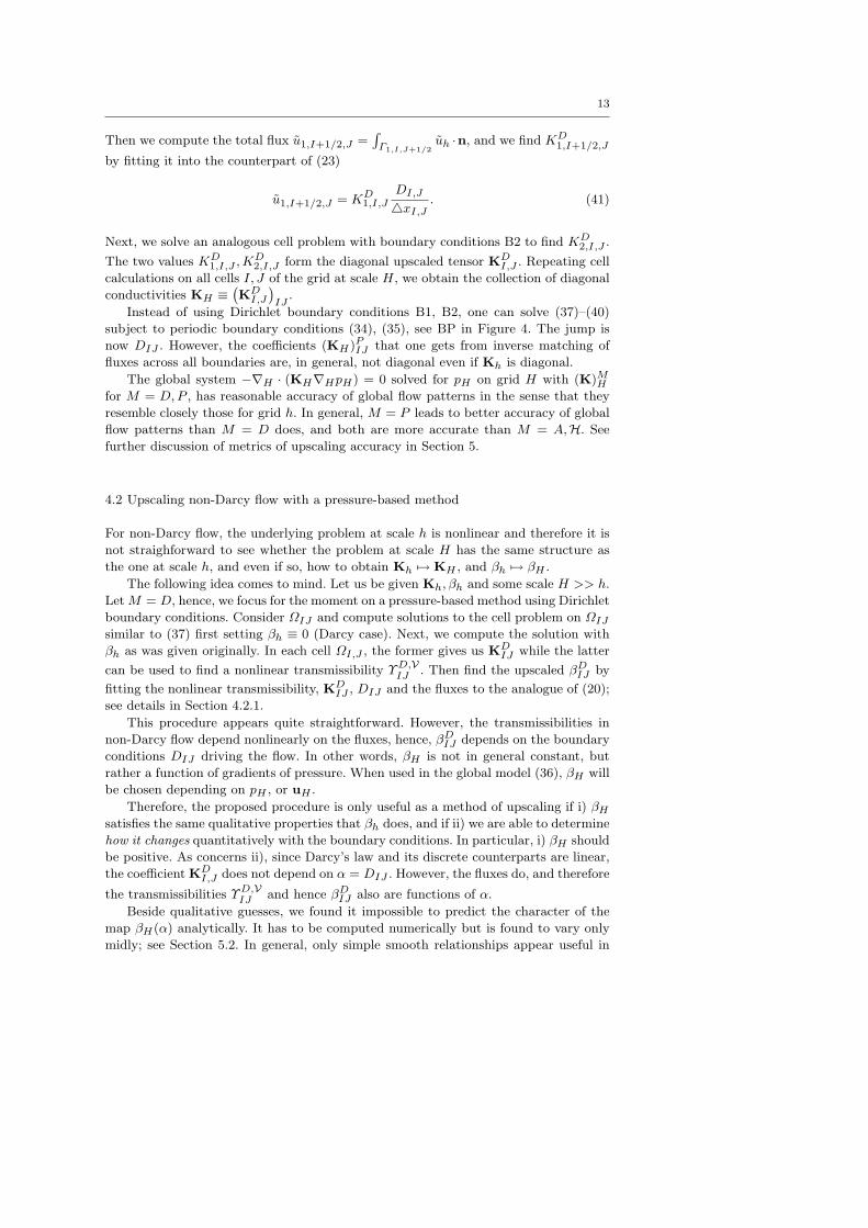
Fig. 5 Field Kh for three cases a) layered, b) periodic (jump of a factor of 10), c) heterogeneous
Consider a 2D region of flow with Kh as shown in Figure 5 with permeability field a)
layered isotropic, b) periodic (similar to a fracture system), and c) small heterogeneous.
For each Kh, let βh be given by (6) with B = 0, 1, and β0 as indicated in each case.
Now solve the problem (53) subject to boundary conditions of type B1, B2, or B3,
as shown in Figure 4, with unit Dirichlet data. In the numerical model we consider
velocity variants V = 0, 1 as in (26). Below follows a discussion of most interesting and
at the same time simple enough cases.
As concerns the layered case a), the results shown earlier in Section 2.1 in Figure 2
c) are representative of cross-sections when Kh is layered and boundary conditions B1
are used. With large β0, the profiles of pressure become more typical of those for a
homogeneous medium. If boundary conditions B2 are used, the flow field is uniform;
we skip the presentation of these results.
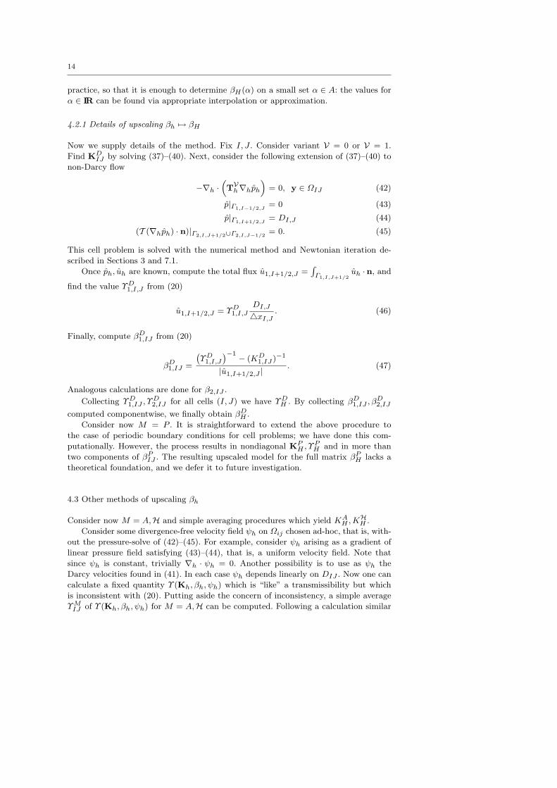
Results for the periodic field b) are shown in Figure 6. Here, we use boundary
conditions B3 in order to make the flow patterns interesting enough. The same effect
of smoothing effects of larger β0 on pressure profiles is observed.
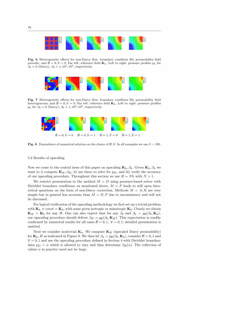
Next we show the effects of the choice of B and of V; we focus on the heterogeneous
case c) and use β0 = 100. See Figure 8, where pressure profiles for different choices of
B,V are shown. It is evident that the solutions for different variants V = 0, 1 do not
differ much; this is also true for other values of β0 (not shown). However, as expected,
the solutions for different B = 0, 1 differ substantially. This suggests that care must be
taken in real simulations to determine an appropriate model (6) of β.
16
0.950.850.750.650.550.450.350.250.15
0.660.60.540.480.420.36
0.660.60.540.480.420.36
0.660.60.540.480.420.36
0.660.60.540.480.420.36
Fig. 6 Heterogeneity effects for non-Darcy flow, boundary condition B3, permeability fieldperiodic, and B = 0,V = 0. Far left: reference field Kh. Left to right: pressure profiles ph forβ0 = 0 (Darcy), β0 = 1, 102, 103, respectively.
0.950.850.750.650.550.450.350.250.15
0.850.750.650.550.450.350.250.15
0.850.750.650.550.450.350.250.15
0.850.750.650.550.450.350.250.15
0.850.750.650.550.450.350.250.15
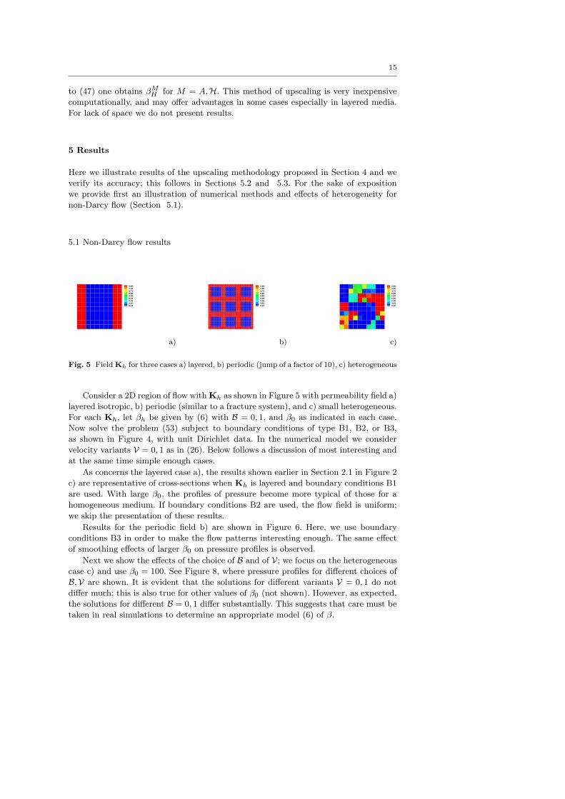
Fig. 7 Heterogeneity effects for non-Darcy flow, boundary condition B3, permeability fieldheterogeneous, and B = 0,V = 0. Far left: reference field Kh. Left to right: pressure profilesph for β0 = 0 (Darcy), β0 = 1, 102, 103, respectively.
0.950.850.750.650.550.450.350.250.15
0.850.750.650.550.450.350.250.15
0.850.750.650.550.450.350.250.15
0.850.750.650.550.450.350.250.15
0.850.750.650.550.450.350.250.15
B = 0,V = 0 B = 0,V = 1 B = 1,V = 0 B = 1,V = 1
Fig. 8 Dependence of numerical solution on the choice of B,V. In all examples we use β = 100.
5.2 Results of upscaling
Now we come to the central issue of this paper on upscaling Kh, βh. Given Kh, βh we
want to i) compute KH , βH , ii) use these to solve for pH , and iii) verify the accuracy
of our upscaling procedure. Throughout this section we use H = Nh with N > 1.
We restrict presentation to the method M = D using pressure-based solver with
Dirichlet boundary conditions; as mentioned above, M = P leads to still open theo-
retical questions on the form of non-Darcy correction. Methods M = A,H are very
simple but in general less accurate than M = D,P due to inconsistency and will not
be discussed.
For logical verification of the upscaling methodology we first set up a trivial problem
with Kh ≡ const = K0, with some given isotropic or anisotropic K0. Clearly we obtain
KH = K0 for any H. One can also expect that for any β0 and βh = gB(β0,Kh),
our upscaling procedure should deliver βH = gB(β0,KH). This expectation is readily
confirmed by numerical results for all cases B = 0, 1, V = 0, 1; detailed presentation is
omitted.
Next we consider nontrivial Kh. We compute KH (upscaled Darcy permeability)
for Kh, H as indicated in Figure 9. We then let βh = gB(β0,Kh), consider B = 0, 1 and
V = 0, 1 and use the upscaling procedure defined in Section 4 with Dirichlet boundary
data pD = α which is allowed to vary and thus determine βH(α). The collection of
values α in practice need not be large.
17
0.90.80.70.60.50.40.30.2
0.90.80.70.60.50.40.30.2
220.180.140.100.60.20.
220.180.140.100.60.20.
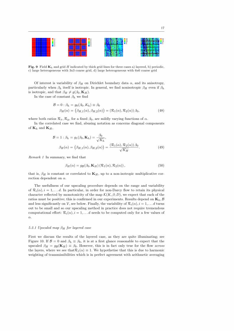
Fig. 9 Field Kh and grid H indicated by thick grid lines for three cases a) layered, b) periodic,c) large heterogeneous with 3x3 coarse grid, d) large heterogeneous with 6x6 coarse grid
Of interest is variability of βH on Dirichlet boundary data α, and its anisotropy,
particularly when βh itself is isotropic. In general, we find nonisotropic βH even if βh
is isotropic, and that βH 6= g(β0,KH).
In the case of constant βh we find
B = 0 : βh = g0(β0,Kh) ≡ β0
βH(α) =(
βH,1(α), βH,2(α))
= (R1(α),R2(α))β0, (48)
where both ratios Rx,Ry, for a fixed β0, are mildly varying functions of α.
In the correlated case we find, abusing notation as concerns diagonal components
of Kh and KH ,
B = 1 : βh = g1(β0,Kh) =β0√Kh
,
βH(α) =(
βH,1(α), βH,2(α))
=(R1(α),R2(α))β0√
KH. (49)
Remark 1 In summary, we find that
βH(α) = gB(β0,KH) (R1(α),R2(α)) , (50)
that is, βH is constant or correlated to KH , up to a non-isotropic multiplicative cor-
rection dependent on α.
The usefullness of our upscaling procedure depends on the range and variability
of Ri(α), i = 1, . . . d. In particular, in order for non-Darcy flow to retain its physical
character reflected by monotonicity of the map K(K,β;D), we expect that each of the
ratios must be positive; this is confirmed in our experiments. Results depend on Kh,Band less significantly on V, see below. Finally, the variability of Ri(α), i = 1, . . . d turns
out to be small and so our upscaling method in practice does not require tremendous
computational effort: Ri(α), i = 1, . . . d needs to be computed only for a few values of
α.
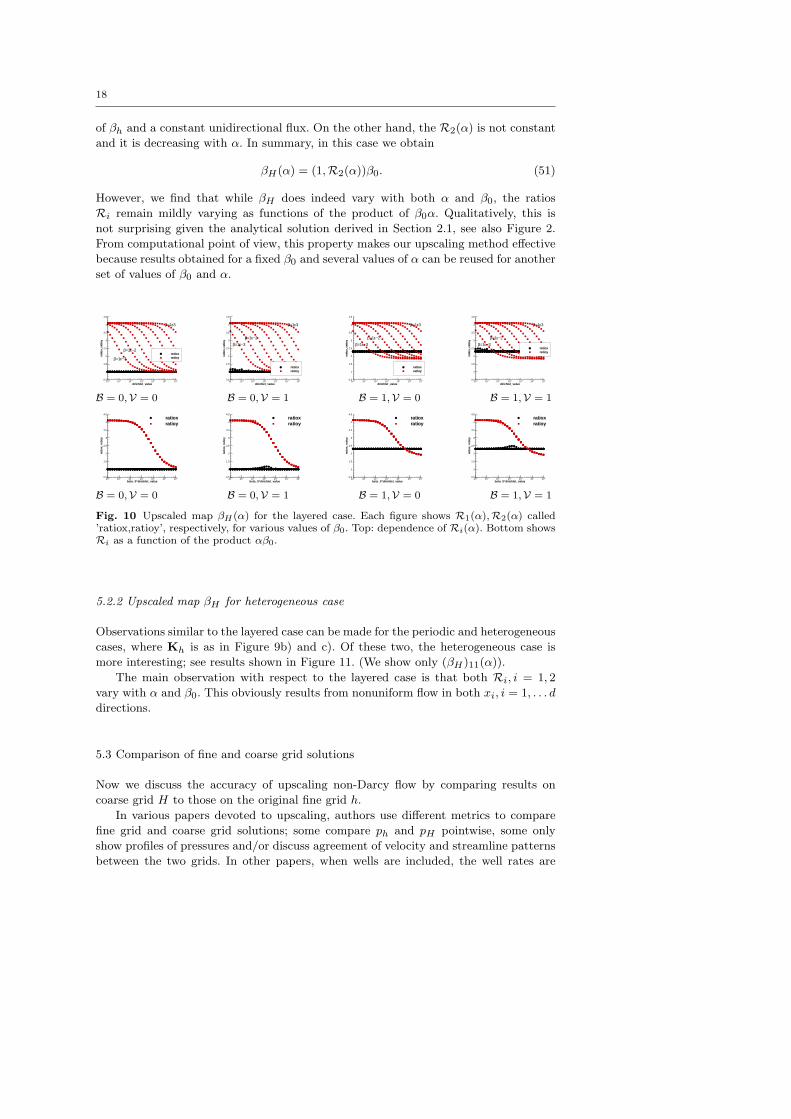
5.2.1 Upscaled map βH for layered case
First we discuss the results of the layered case, as they are quite illuminating; see
Figure 10. If B = 0 and βh ≡ β0, it is at a first glance reasonable to expect that the
upscaled βH = gB(KH) ≡ β0. However, this is in fact only true for the flow across
the layers, where we see thatR1(α) ≡ 1. We hypothetise that this is due to harmonic
weighting of transmissibilities which is in perfect agreement with arithmetic averaging
18
of βh and a constant unidirectional flux. On the other hand, the R2(α) is not constant
and it is decreasing with α. In summary, in this case we obtain
βH(α) = (1,R2(α))β0. (51)
However, we find that while βH does indeed vary with both α and β0, the ratios
Ri remain mildly varying as functions of the product of β0α. Qualitatively, this is
not surprising given the analytical solution derived in Section 2.1, see also Figure 2.
From computational point of view, this property makes our upscaling method effective
because results obtained for a fixed β0 and several values of α can be reused for another
set of values of β0 and α.
dirichlet_value
ratio
x,ra
tioy
10-3 10-2 10-1 100 101 102 1030.5
1
1.5
2
2.5
3
3.5
4
4.5
ratioxratioy
β=1ε3
β=1ε−3
β=1ε−2
dirichlet_value
ratio
x,ra
tioy
10-3 10-2 10-1 100 101 102 1030.5
1
1.5
2
2.5
3
3.5
4
4.5
ratioxratioy
β=1ε3
β=1ε−3β=1ε−2
dirichlet_value
ratio
x,ra
tioy
10-3 10-2 10-1 100 101 102 1030.5
1
1.5
2
2.5
3
3.5
4
4.5
ratioxratioy
β=1ε3
β=1ε−3β=1ε−2
dirichlet_value
ratio
x,ra
tioy
10-3 10-2 10-1 100 101 102 1030.5
1
1.5
2
2.5
3
3.5
4
4.5
ratioxratioy
β=1ε3
β=1ε−3β=1ε−2
B = 0,V = 0 B = 0,V = 1 B = 1,V = 0 B = 1,V = 1
beta_0*dirichlet_value
ratio
x,ra
tioy
10-3 10-2 10-1 100 101 102 1030.5
1
1.5
2
2.5
3
3.5
4
4.5
ratioxratioy
beta_0*dirichlet_value
ratio
x,ra
tioy
10-3 10-2 10-1 100 101 102 1030.5
1
1.5
2
2.5
3
3.5
4
4.5
ratioxratioy
beta_0*dirichlet_value
ratio
x,ra
tioy
10-3 10-2 10-1 100 101 102 1030.5
1
1.5
2
2.5
3
3.5
4
4.5
ratioxratioy
beta_0*dirichlet_value
ratio
x,ra
tioy
10-3 10-2 10-1 100 101 102 1030.5
1
1.5
2
2.5
3
3.5
4
4.5
ratioxratioy
B = 0,V = 0 B = 0,V = 1 B = 1,V = 0 B = 1,V = 1
Fig. 10 Upscaled map βH(α) for the layered case. Each figure shows R1(α),R2(α) called’ratiox,ratioy’, respectively, for various values of β0. Top: dependence of Ri(α). Bottom showsRi as a function of the product αβ0.
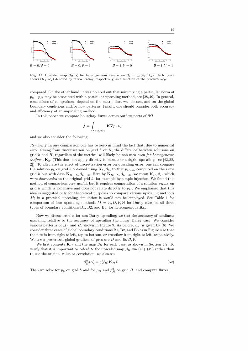
5.2.2 Upscaled map βH for heterogeneous case
Observations similar to the layered case can be made for the periodic and heterogeneous
cases, where Kh is as in Figure 9b) and c). Of these two, the heterogeneous case is
more interesting; see results shown in Figure 11. (We show only (βH)11(α)).
The main observation with respect to the layered case is that both Ri, i = 1, 2
vary with α and β0. This obviously results from nonuniform flow in both xi, i = 1, . . . d
directions.
5.3 Comparison of fine and coarse grid solutions
Now we discuss the accuracy of upscaling non-Darcy flow by comparing results on
coarse grid H to those on the original fine grid h.
In various papers devoted to upscaling, authors use different metrics to compare
fine grid and coarse grid solutions; some compare ph and pH pointwise, some only
show profiles of pressures and/or discuss agreement of velocity and streamline patterns
between the two grids. In other papers, when wells are included, the well rates are
19
beta_0*dirichlet_value
ratio
x,ra
tioy
10-3 10-2 10-1 100 101 102 103
1.5
2
2.5
3
3.5
4
4.5
5
ratioxratioy
beta_0*dirichlet_value
ratio
x,ra
tioy
10-3 10-2 10-1 100 101 102 103
1.5
2
2.5
3
3.5
4
4.5
5
ratioxratioy
beta_0*dirichlet_value
ratio
x,ra
tioy
10-3 10-2 10-1 100 101 102 103
1.5
2
2.5
3
3.5
4
4.5
5
ratioxratioy
beta_0*dirichlet_value
ratio
x,ra
tioy
10-3 10-2 10-1 100 101 102 103
1.5
2
2.5
3
3.5
4
4.5
5
ratioxratioy
B = 0,V = 0 B = 0,V = 1 B = 1,V = 0 B = 1,V = 1
Fig. 11 Upscaled map βH(α) for heterogeneous case when βh = gB(β0,Kh). Each figureshows (R1,R2) denoted by ratiox, ratioy, respectively, as a function of the product αβ0.
compared. On the other hand, it was pointed out that minimizing a particular norm of
ph − pH may be associated with a particular upscaling method, see [28,49]. In general,
conclusions of comparisons depend on the metric that was chosen, and on the global
boundary conditions and/or flow patterns. Finally, one should consider both accuracy
and efficiency of an unpscaling method.
In this paper we compare boundary fluxes across outflow parts of ∂Ω
f =
∫
Γoutflow
K∇p · ν,
and we also consider the following.
Remark 2 In any comparison one has to keep in mind the fact that, due to numerical
error arising from discretization on grid h or H, the difference between solutions on
grid h and H, regardless of the metrics, will likely be non-zero even for homogeneous
uniform Kh. (This does not apply directly to mortar or subgrid upscaling; see [42,38,
2]). To alleviate the effect of discretization error on upscaling error, one can compare
the solution ph on grid h obtained using Kh, βh, to that pH 7→h computed on the same
grid h but with data KH 7→h, βH 7→h. Here by KH 7→h, βH 7→h, we mean KH , βH which
were downscaled to the original grid h, for example by simple injection. We found this
method of comparison very useful, but it requires computation of a solution pH 7→h on
grid h which is expensive and does not relate directly to pH . We emphasize that this
idea is suggested only for theoretical purposes to compare various upscaling methods
M ; in a practical upscaling simulation it would not be employed. See Table 1 for
comparison of four upscaling methods M = A,D, P,H for Darcy case for all three
types of boundary conditions B1, B2, and B3, for heterogeneous Kh.
Now we discuss results for non-Darcy upscaling; we test the accuracy of nonlinear
upscaling relative to the accuracy of upscaling the linear Darcy case. We consider
various patterns of Kh and H, shown in Figure 9. As before, βh, is given by (6). We
consider three cases of global boundary conditions B1, B2, and B3 as in Figure 4 so that
the flow is from right to left, top to bottom, or crossflow from right to left, respectively.
We use a prescribed global gradient of pressure D and fix B,V.
We first compute KH and the map βH for each case, as shown in Section 5.2. To
verify that it is important to calculate the upscaled map βH via (48)–(49) rather than
to use the original value or correlation, we also set
βgH(α) = g(β0;KH). (52)
Then we solve for ph on grid h and for pH and pgH on grid H, and compute fluxes.
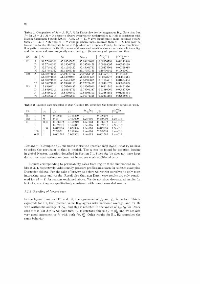
20
Table 1 Comparison of M = A, D, P,H for Darcy flow for heterogeneous Kh. Note that fluxfH for M = A / M = H seems to always overpredict/ underpredict fh; this is consistent withHashin-Shtrikman bounds [29,45]. Also, M = D, P give significantly more accurate resultsthan M = A,H. Note that M = P while in general more accurate than M = D here may beless so due to the off-diagonal terms of KP
Hwhich are dropped. Finally, for more complicated
flow pattern associated with B3, the use of downscaled solution shows that the coefficients KH
and the numerical error are jointly contributing to (in)accuracy of upscaled solution.
BC M fh fH fH 7→h |fh−fH
fh| |
fh−fH 7→hfh
|
B1 A 32.57484362 55.03545873 55.09824639 0.68950799 0.69143548D 32.57484362 32.35069719 32.38584459 0.00688097 0.00580199P 32.57484362 32.41986422 32.45464733 0.00475764 0.00368985H 32.57484362 26.14566346 26.17359339 0.19736642 0.19650901
B2 A 51.38471961 58.92646422 58.97261428 0.14677018 0.14766831D 51.38471961 51.34424224 51.38080698 0.00078773 0.00007614P 51.38471961 50.55448835 50.58589065 0.01615716 0.01554604H 51.38471961 35.73207110 35.77021427 0.30461679 0.30387449
B3 A 17.85362214 20.76764487 26.32567940 0.16321745 0.47452876D 17.85362214 13.98183753 17.75764287 0.21686269 0.00537590P 17.85362214 13.85705590 17.63303101 0.22385184 0.01235554H 17.85362214 10.29882863 12.91371346 0.42315186 0.27668944
Table 2 Layered case upscaled to 2x2. Column BC describes the boundary condition used.
BC D β0 fh fH |fh−fH
fh| f
g
H|fh−f
gH
fh|
B1 1 0 0.15625 0.156250 0 0.156250 0B2 1 0 0.46 0.460000 1.2e-016 0.460000 1.2e-016B1 1 0.01 0.156212 0.156212 1.4e-013 0.156212 1.4e-013
1 1 0.152611 0.152611 2.9e-015 0.152611 2.9e-0151 100 0.072995 0.072995 1.9e-016 0.072995 1.9e-016100 1 7.29952 7.299524 2.4e-016 7.299524 2.4e-0160.01 1 0.001562 0.001562 1.4e-013 0.001562 1.4e-013
Remark 3 To compute pH , one needs to use the upscaled map βH(α), that is, we have
to select the particular α that is needed. The α can be found by iteration lagging
in global Newton iteration described in Section 7.1. Since βH(α) does not have large
derivatives, such estimation does not introduce much additional error.
Results corresponding to permeability cases from Figure 9 are summarized in Ta-
bles 2, 3, 4, respectively. Additionally, pressure profiles are shown for selected examples.
Discussion follows. For the sake of brevity as before we restrict ourselves to only most
interesting cases and results. Recall also that non-Darcy case results are only consid-
ered for M = D for reasons explained above. We do not show downscaled results for
lack of space; they are qualitatively consistent with non-downscaled results.
5.3.1 Upscaling of layered case
In the layered case and B1 and B2, the agreement of fh and fH is perfect. This is
expected: for B1, the upscaled value KH agrees with harmonic average, and for B2
with arithmetic average of Kh, and this is reflected in the values of fh, fH for Darcy
case β = 0. For β 6= 0, we have that βH is constant and so pH = pgH and we see also
very good agreement of fh with both fH , fgH . Other results for B1, B2 reproduce the
same behavior.
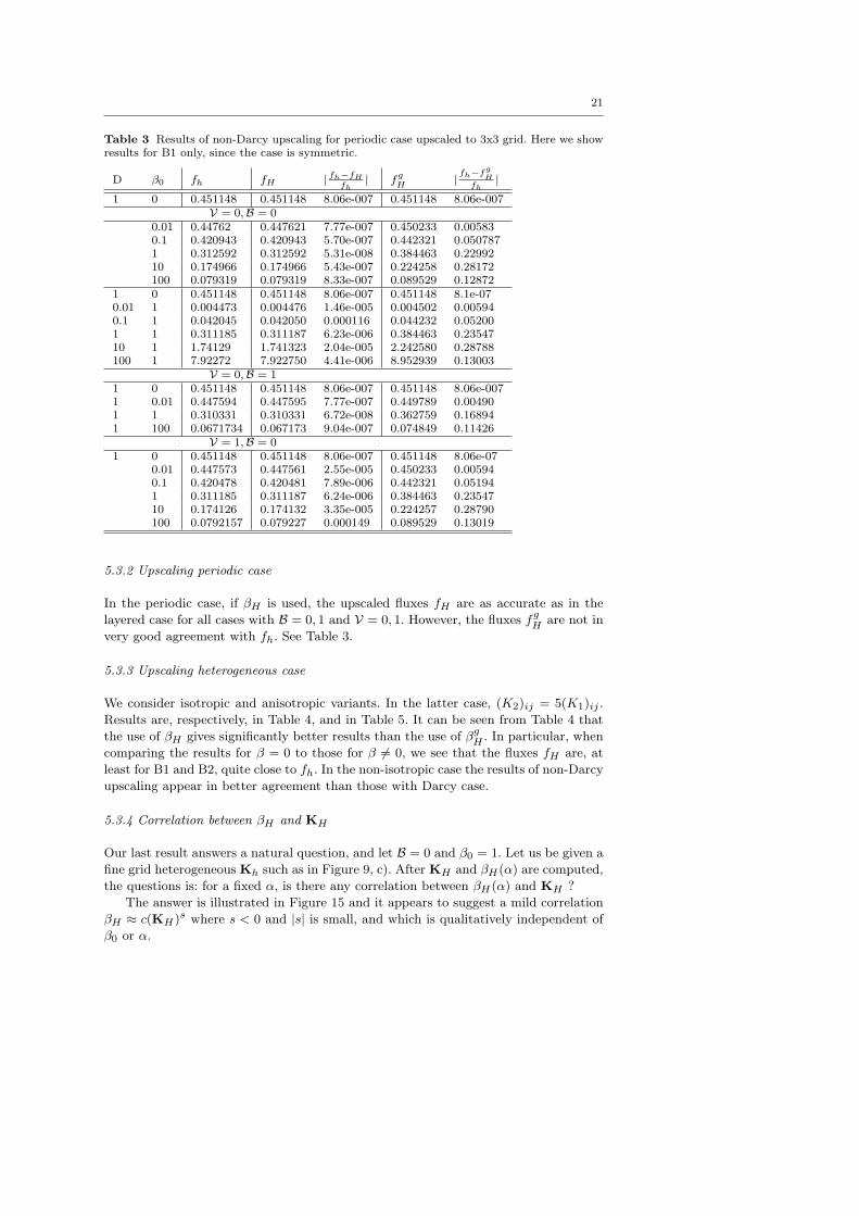
21
Table 3 Results of non-Darcy upscaling for periodic case upscaled to 3x3 grid. Here we showresults for B1 only, since the case is symmetric.
D β0 fh fH |fh−fH
fh| f
g
H|fh−f
gH
fh|
1 0 0.451148 0.451148 8.06e-007 0.451148 8.06e-007V = 0,B = 0
0.01 0.44762 0.447621 7.77e-007 0.450233 0.005830.1 0.420943 0.420943 5.70e-007 0.442321 0.0507871 0.312592 0.312592 5.31e-008 0.384463 0.2299210 0.174966 0.174966 5.43e-007 0.224258 0.28172100 0.079319 0.079319 8.33e-007 0.089529 0.12872
1 0 0.451148 0.451148 8.06e-007 0.451148 8.1e-070.01 1 0.004473 0.004476 1.46e-005 0.004502 0.005940.1 1 0.042045 0.042050 0.000116 0.044232 0.052001 1 0.311185 0.311187 6.23e-006 0.384463 0.2354710 1 1.74129 1.741323 2.04e-005 2.242580 0.28788100 1 7.92272 7.922750 4.41e-006 8.952939 0.13003
V = 0,B = 11 0 0.451148 0.451148 8.06e-007 0.451148 8.06e-0071 0.01 0.447594 0.447595 7.77e-007 0.449789 0.004901 1 0.310331 0.310331 6.72e-008 0.362759 0.168941 100 0.0671734 0.067173 9.04e-007 0.074849 0.11426
V = 1,B = 01 0 0.451148 0.451148 8.06e-007 0.451148 8.06e-07
0.01 0.447573 0.447561 2.55e-005 0.450233 0.005940.1 0.420478 0.420481 7.89e-006 0.442321 0.051941 0.311185 0.311187 6.24e-006 0.384463 0.2354710 0.174126 0.174132 3.35e-005 0.224257 0.28790100 0.0792157 0.079227 0.000149 0.089529 0.13019
5.3.2 Upscaling periodic case
In the periodic case, if βH is used, the upscaled fluxes fH are as accurate as in the
layered case for all cases with B = 0, 1 and V = 0, 1. However, the fluxes fgH are not in
very good agreement with fh. See Table 3.
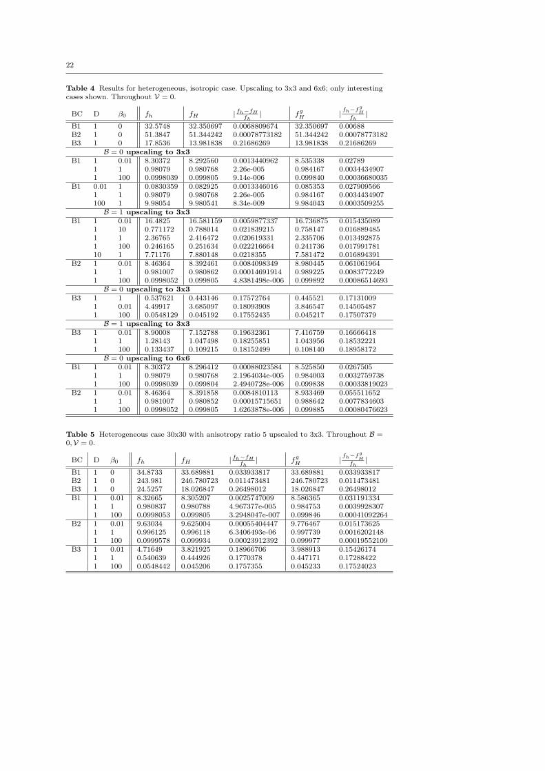
5.3.3 Upscaling heterogeneous case
We consider isotropic and anisotropic variants. In the latter case, (K2)ij = 5(K1)ij .
Results are, respectively, in Table 4, and in Table 5. It can be seen from Table 4 that
the use of βH gives significantly better results than the use of βgH . In particular, when
comparing the results for β = 0 to those for β 6= 0, we see that the fluxes fH are, at
least for B1 and B2, quite close to fh. In the non-isotropic case the results of non-Darcy
upscaling appear in better agreement than those with Darcy case.
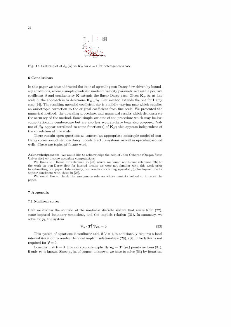
5.3.4 Correlation between βH and KH
Our last result answers a natural question, and let B = 0 and β0 = 1. Let us be given a
fine grid heterogeneous Kh such as in Figure 9, c). After KH and βH(α) are computed,
the questions is: for a fixed α, is there any correlation between βH(α) and KH ?
The answer is illustrated in Figure 15 and it appears to suggest a mild correlation
βH ≈ c(KH)s where s < 0 and |s| is small, and which is qualitatively independent of
β0 or α.
22
Table 4 Results for heterogeneous, isotropic case. Upscaling to 3x3 and 6x6; only interestingcases shown. Throughout V = 0.
BC D β0 fh fH |fh−fH
fh| f
g
H|fh−f
gH
fh|
B1 1 0 32.5748 32.350697 0.0068809674 32.350697 0.00688B2 1 0 51.3847 51.344242 0.00078773182 51.344242 0.00078773182B3 1 0 17.8536 13.981838 0.21686269 13.981838 0.21686269
B = 0 upscaling to 3x3
B1 1 0.01 8.30372 8.292560 0.0013440962 8.535338 0.027891 1 0.98079 0.980768 2.26e-005 0.984167 0.00344349071 100 0.0998039 0.099805 9.14e-006 0.099840 0.00036680035
B1 0.01 1 0.0830359 0.082925 0.0013346016 0.085353 0.0279095661 1 0.98079 0.980768 2.26e-005 0.984167 0.0034434907100 1 9.98054 9.980541 8.34e-009 9.984043 0.0003509255
B = 1 upscaling to 3x3
B1 1 0.01 16.4825 16.581159 0.0059877337 16.736875 0.0154350891 10 0.771172 0.788014 0.021839215 0.758147 0.0168894851 1 2.36765 2.416472 0.020619331 2.335706 0.0134928751 100 0.246165 0.251634 0.022216664 0.241736 0.01799178110 1 7.71176 7.880148 0.0218355 7.581472 0.016894391
B2 1 0.01 8.46364 8.392461 0.0084098349 8.980445 0.0610619641 1 0.981007 0.980862 0.00014691914 0.989225 0.00837722491 100 0.0998052 0.099805 4.8381498e-006 0.099892 0.00086514693
B = 0 upscaling to 3x3
B3 1 1 0.537621 0.443146 0.17572764 0.445521 0.171310091 0.01 4.49917 3.685097 0.18093908 3.846547 0.145054871 100 0.0548129 0.045192 0.17552435 0.045217 0.17507379
B = 1 upscaling to 3x3
B3 1 0.01 8.90008 7.152788 0.19632361 7.416759 0.166664181 1 1.28143 1.047498 0.18255851 1.043956 0.185322211 100 0.133437 0.109215 0.18152499 0.108140 0.18958172
B = 0 upscaling to 6x6
B1 1 0.01 8.30372 8.296412 0.00088023584 8.525850 0.02675051 1 0.98079 0.980768 2.1964034e-005 0.984003 0.00327597381 100 0.0998039 0.099804 2.4940728e-006 0.099838 0.00033819023
B2 1 0.01 8.46364 8.391858 0.0084810113 8.933469 0.0555116521 1 0.981007 0.980852 0.00015715651 0.988642 0.00778346031 100 0.0998052 0.099805 1.6263878e-006 0.099885 0.00080476623
Table 5 Heterogeneous case 30x30 with anisotropy ratio 5 upscaled to 3x3. Throughout B =0,V = 0.
BC D β0 fh fH |fh−fH
fh| f
g
H|fh−f
gH
fh|
B1 1 0 34.8733 33.689881 0.033933817 33.689881 0.033933817B2 1 0 243.981 246.780723 0.011473481 246.780723 0.011473481B3 1 0 24.5257 18.026847 0.26498012 18.026847 0.26498012B1 1 0.01 8.32665 8.305207 0.0025747009 8.586365 0.031191334
1 1 0.980837 0.980788 4.967377e-005 0.984753 0.00399283071 100 0.0998053 0.099805 3.2948047e-007 0.099846 0.00041092264
B2 1 0.01 9.63034 9.625004 0.00055404447 9.776467 0.0151736251 1 0.996125 0.996118 6.3406493e-06 0.997739 0.00162021481 100 0.0999578 0.099934 0.00023912392 0.099977 0.00019552109
B3 1 0.01 4.71649 3.821925 0.18966706 3.988913 0.154261741 1 0.540639 0.444926 0.1770378 0.447171 0.172884221 100 0.0548442 0.045206 0.1757355 0.045233 0.17524023
23
220.180.140.100.60.20.
75.65.55.45.35.25.15.
75.65.55.45.35.25.15.
100.16100.14100.12100.1100.08100.06100.04100.02
100.505100.445100.385100.325100.265100.205100.145100.085100.025
24.22.20.18.16.14.12.
19.518.517.516.515.514.513.512.511.5
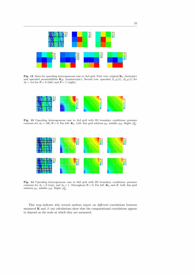
Fig. 12 Data for upscaling heterogeneous case to 3x3 grid. First row: original Kh (isotropic)and upscaled permeabilities KH (nonisotropic). Second row: upscaled β1,H(1), β2,H(1) forβ0 = 1e2 for B = 0 (left) and B = 1 (right).
220.180.140.100.60.20.
0.70.680.660.640.620.60.580.560.540.520.50.480.460.440.420.40.380.36
0.70.680.660.640.620.60.580.560.540.520.50.480.460.440.420.40.380.36
0.70.680.660.640.620.60.580.560.540.520.50.480.460.440.420.40.380.36
Fig. 13 Upscaling heterogeneous case to 3x3 grid with B3 boundary conditions: pressurecontours for β0 = 100, B = 0. Far left: Kh. Left: fine grid solution ph, middle: pH . Right: p
g
H.
220.180.140.100.60.20.
0.850.750.650.550.450.350.250.15
0.850.750.650.550.450.350.250.15
0.850.750.650.550.450.350.250.15
220.180.140.100.60.20.
0.850.750.650.550.450.350.250.15
0.850.750.650.550.450.350.250.15
0.850.750.650.550.450.350.250.15
Fig. 14 Upscaling heterogeneous case to 6x6 grid with B3 boundary conditions: pressurecontours for β0 = 0 (top), and β0 = 1. Throughout B = 0. Far left: Kh and H. Left: fine gridsolution ph, middle: pH . Right: p
g
H.
This may indicate why several authors report on different correlations between
measured K and β; our calculations show that the computational correlations appear
to depend on the scale at which they are measured.
24
Kx, Ky
β x,β y
20 40 60 80 100 1201
1.005
1.01
1.015
1.02 βx(Kx)βy(Ky)
Fig. 15 Scatter-plot of βH(α) vs KH for α = 1 for heterogeneous case.
6 Conclusions
In this paper we have addressed the issue of upscaling non-Darcy flow driven by bound-
ary conditions, where a simple quadratic model of velocity parametrized with a positive
coefficient β and conductivity K extends the linear Darcy case. Given Kh, βh at fine
scale h, the approach is to determine KH , βH . Our method extends the one for Darcy
case [14]. The resulting upscaled coefficient βH is a mildly varying map which supplies
an anisotropic correction to the original coefficient from fine scale. We presented the
numerical method, the upscaling procedure, and numerical results which demonstrate
the accuracy of the method. Some simple variants of the procedure which may be less
computationally cumbersome but are also less accurate have been also proposed. Val-
ues of βH appear correlated to some function(s) of KH ; this appears independent of
the correlation at fine scale.
There remain open questions as concern an appropriate anistropic model of non-
Darcy correction, other non-Darcy models, fracture systems, as well as upscaling around
wells. These are topics of future work.
Acknowledgements We would like to acknowledge the help of John Osborne (Oregon StateUniversity) with some upscaling computations.
We thank Jill Reese for reference to [44] where we found additional reference [26] tothe work on non-Darcy flow for layered media; we were not familiar with this work priorto submitting our paper. Interestingly, our results concerning upscaled βH for layered mediaappear consistent with those in [26].
We would like to thank the anonymous referees whose remarks helped to improve thepaper.
7 Appendix
7.1 Nonlinear solver
Here we discuss the solution of the nonlinear discrete system that arises from (22),
some imposed boundary conditions, and the implicit relation (31). In summary, we
solve for ph the system
∇h · TVh∇ph = 0. (53)
This system of equations is nonlinear and, if V = 1, it additionally requires a local
internal iteration to resolve the local implicit relationships (29), (30). The latter is not
required for V = 0.
Consider first V = 0. One can compute explicitly uh = T0(ph) pointwise from (31),
if only ph is known. Since ph is, of course, unknown, we have to solve (53) by iteration.
25
As initial guess p(0)h one can use the Darcy pressures which can be found by solving
a linear counterpart of (53) setting β = 0. Or, for large β, additionally one may try
the method of continuity in which one starts with β = 0 and then iterates, gradually
increasing β to the desired magnitude, thereby obtaining a better initial guess.
It appears very natural to solve (53) using successive substitutions iterating on
(31). Unfortunately, for small h and large heterogeneities, this simple iteration may
have trouble converging and/or is very slow. The only reasonable alternative is to use
Newton’s method. We set it up as follows.
Given an initial guess p(0)h , iterate for n = 0, 1, . . . until convergence
(∗) compute u(n)h = TV
(
Kh, βh, |u(n)h |,u(n)
h
)
∇hp(n)h
compute residual R(n) = ∇h · u(n)h
compute Jacobian J(n) =∂
∂phR(n)
advance p(n+1)h = p
(n)h − (J(n))−1R(n)
In this algorithm, the step (∗) can be executed pointwise analytically, if V = 0. The
residual calculations of R(n) are quite simple as we only have to calculate the current
∇h ·u(n)h . Jacobian calculations of J(n) are done with the help of (12). Overall however,
the method converges generally quite fast, even for large β.
Consider now V = 1. Now the step (∗) cannot be executed exactly and, in order to
resolve (21), we compute an iteration-lagged approximation u(n)h to u
(n)h via
u(n)h = TV
(
Kh, βh, |u(n−1)h |, u(n)
h
)
∇hp(n)h .
This introduces a mild inconsistency in the residual and Jacobian calculations. How-
ever, the Newton iteration converges at least as fast as the one for V = 0. If the
iteration is run under strict convergence tolerance criteria, then one can assume that
u(n)h ≈ u
(n)h . Note that due to a different formulation ph,uh obtained with V = 0, 1
are (somewhat) different, see results shown in Section 5.
Our experience with performance of the Newton solver for variants V = 0, 1, models
B = 0, 1 of βh and values of Kh can be summarized as follows. The solver needs more
iterations in the case of strong anisotropy especially if β is correlated with K. Next, one
should formulate the stopping criteria very carefully: in terms of simple mass-balanced
residual norms, the iteration appears not to be making much progress, while pressure
and velocity values have not yet converged. As concerns velocity variants, variant V = 0
requires more iterations to converge than V = 1, especially for strong anisotropy ratio
and large uncorrelated heterogeneities; this is likely caused by V = 1 being capable
of carrying more information. The opposite appears true for small correlation lengths,
for example for the periodic fissure problem (see Section 5) and is probably due to the
inconsistency of residuals discussed above playing more substantial role in the absence
of other difficulties.
7.2 Mixed FE derivation of (25)
Here we use mixed finite elements of type RT[0] on a rectangular grid to derive (25);
we focus on details leading to (26). Such derivation was done for Darcy’s flow in [46].
26
The non-Darcy flow equations were discretized using mixed FE in [12,36] but, to our
knowledge, the use of quadrature and identification with CCFD discussed here has not
been carried out. The importance of this derivation is that it extends the convergence
results of mixed FE to CCFD formulation; on the other hand, it uncouples the saddle
point formulation of mixed FE [46]. For notation see also [6].
First consider the weak formulation of (1), (4) complemented by no-flow boundary
conditions (33) with ΓN ≡ ∂Ω. Let (W,V) = (L2(Ω), v ∈ H(div;Ω) : v · ν|ΓN= 0).
The weak solution (p,u) ∈ (W,V) satisfies the system obtained by by multiplying (4),
(1) by test functions w ∈W,v ∈ V and integrating by parts over Ω
∫
Ω
∇ · uw =
∫
Ω
qw, ∀w ∈W, (54)
∫
Ω
K−1u · v +
∫
Ω
β|u|u · v =
∫
Ω
p∇ · v, ∀v ∈ V (55)
The mixed FE solution (ph,uh) ∈Wh×Vh whereWh ⊂W,Vh ⊂ V. The functions
in Wh are piecewise constant on each cell; a test function ξij ∈ Wh is a characteristic
function of the cell Ωi,j so that ph(x, y) =∑
ij ξij(x, y)pij . Recall that the functions
vh ∈ Vh from space RT[0] [43] are piecewise linear in one coordinate direction and
piecewise constant in the others and can be written symbolically as a tensor product
RT[0] = P1,0 × P0,1 [6][46,43]. Here Pq,r(S) denotes a space of polynomials of degree
q in x1 and of degree r in x2 which are variables over a subset S ⊂ IRd. We have
uh(x, y)|Ωij=(
ψi−1/2,j(x)ui−1/2,j + ψi+1/2,j(x)ui+1/2,j ,
φi,j−1/2(y)vi,j−1/2 + φi,j+1/2(y)vi,j+1/2
)
,
with the basis functions ψi+/−1/2,j(x), φi,j+/−1/2(y) in P1,0 and P0,1, respectively.
Note that ψi+1/2,j(x) is supported only on Ωij ∪Ωi+1,j .
It is also useful to consider the value of uh on the edge Ei+1/2,j,k = ∂Ωij∩∂Ωi+1,j .
By definition of uh, we are guaranteed the continuity of its normal component (uh)1but not of its tangential component (uh)2 across that edge. The discrete solution
(ph,uh) satisfies an equation analogous to (54) in which
∫
Ω
∇ · uhwh =
∫
Ω
qwh, ∀wh ∈Wh,
and using wh = ξij one derives pointwise
ui+1/2,j − ui−1/2,j + ui,j+1/2 − ui,j−1/2 = qij xi yj , (56)
which can be interpretted as (22) when q ≡ 0. The discrete analogue to momentum
equation (55) is
∫
Ω
K−1h uh · vh +
∫
Ω
βh|uh|uh · vh =
∫
Ω
ph∇ · vh, ∀vh ∈ Vh (57)
forming a linear saddle-point system along with (22).
Now, as shown in [46] for Darcy flow, the integrals in (57) can be replaced by
their numerical approximations, namely, a combination of trapezoidal and midpoint
quadrature rules, at the expense of introducing a quadrature error of higher order than
approximation order. In this way the discrete velocity values are identified with those in
27
CCFD formulation; the numerical integration approach entirely decouples the original
saddle-point system and allows to solve a symmetric non-negative-definite system in
ph unknown only. We notice that this is possible for diagonal K.
We follow the same idea here for non-Darcy flow. Use the test function vh =
(ψi+1/2,j , ξjk) ∈ Vh and integrate over its support Ωij ∪ Ωi+1,j , with the trapezoidal
rule applied to integration in x1 direction and the midpoint rule applied in y1 directions,
which we denote by subscripts (TM).
The integration rules used below for products are all of second order accuracy with
respect to the size of domain: trapezoidal(
∫ b
af(t)g(t)dt
)
T= (b− a)
f(a)g(a)+f(b)g(b)2 ,
the midpoint rule(
∫ b
af(t)g(t)dt
)
M= (b − a)f(a+b
2 )g(a+b2 ). Additionally, we define
the product P rule as(
∫ b
af(t)g(t)dt
)
P= (b−a)f(a+b
2 )g(a)+g(b)
2 . One can show using
standard numerical analysis that the P rule has (at least) the same order of accuracy
as the trapezoidal rule.
Using the (TM) rule for the first integral on left hand side, and integrating directly
the right hand side of (57) we obtain expressions as in Darcy’s case, since vh equals
zero on both edges Ei−1/2,j , Ei+3/2,j
(∫
Ω
K−1uh · vh
)
TM
=
(
∫
Ωij
K−11,ijuh · vh
)
TM
+
(
∫
Ωi+1,j
K−11,i+1,juh · vh
)
TM
= yjT−11,i+1/2,jui+1/2,jk,
∫
Ω
ph∇ · vh =
∫
Ωij
pij∇ · vh +
∫
Ωi+1,j
pi+1,j∇ · vh = yj(pij − pi+1,j).
The new and most important element in the non-Darcy case is handling of the
second term on the left side of (57). Using the (TM) quadrature rule over Ωij ∪Ωi+1,j ,
we get
(∫
Ω
β|uh|uh · vh
)
TM
= βij
(
∫
Ωij
|uh|uh · v)
TM
+ βi+1,j
(
∫
Ωi+1,j
|uh|u · v)
TM
(58)
Consider one of the integrals on the right side, which gives exactly
(
∫
Ωij
|uh|uh · v)
TM
=xi yj
2|(uh)+ij |u1,i+1/2,j , (59)
and which is consistent with V = 2 in (26) and the following expression
(
T−11,i+1/2,j +
1
2
(
xiβ1,ij |uh|+ij + xi+1β1,i+1,j |uh|−i+1,j
)
)
u1,i+1/2,j (60)
= pi,j − pi+1,j .
Since each |uh|+ij , |uh|−ij depends on u1,i+1/2,j and on other velocity degress of freedom,
as mentioned before, the solution u1,i+1/2,j cannot be obtained analytically or even
by local iteration.
28
This issue can be somewhat rectified by the use, instead of the discontinuous values
|uh|+ij , |uh|−ij in (60), of their average |uh|ij as in V = 1 leading to
(
T−11,i+1,j +
1
2(xiβ1,ij + xi+1β1,i+1,j)|
(uh)+ij + (uh)−i+1,j
2|)
u1,i+1/2,j
= pi,j − pi+1,j . (61)
This introduces an additional error which is however readily seen to be of order not
exceeding that of numerical integration, via expansion, for any z,√
1 + z = 1 + z2 −
18z
2 +O(z3). Further details will not be provided as they are not essential.
Now we discuss V = 3. This arises if in (58) one uses the (PM) integration rule
instead of (TM),
(
∫
Ωij
|uh|uh · v)
PM
=xi yj
2|(uh)ij |u1,i+1/2,j
which provides the following alternative to (27),
(
T−11,i+1/2,j +
1
2
(
xiβ1,ij |(uh)ij | + xi+1β1,i+1,j |(uh)i+1,j |)
)
u1,i+1/2,j
= pi,j − pi+1,j .
Since this formulation leads to an excessively wide stencil, it is not pursued here.
Finally we interpret V = 0. It arises if instead of (7) one discretizes (8). Alter-
natively, V = 0 can be seen as an approximation to V = 1 in which the tangential
components of velocity are ignored.
References
1. Special issue devoted to upscaling in porous media. Computational Geosciences 6 (2002)2. Arbogast, T.: An overview of subgrid upscaling for elliptic problems in mixed form. In:
Current trends in scientific computing (Xi’an, 2002), Contemp. Math., vol. 329, pp. 21–32.Amer. Math. Soc., Providence, RI (2003)
3. Barker, J., Thibeau, S.: A criticial review of the use of pseudo relative permeabilities forupscaling. SPE 35491 (1996)
4. Bear, J.: Dynamics of Fluids in Porous Media. Dover, New York (1972)5. Bensoussan, A., Lions, J.L., Papanicolaou, G.: Asymptotic analysis for periodic struc-
tures, Studies in Mathematics and its Applications, vol. 5. North-Holland Publishing Co.,Amsterdam (1978)
6. Brezzi, F., Fortin, M.: Mixed and hybrid finite element methods, Springer Series in Com-
putational Mathematics, vol. 15. Springer-Verlag, New York (1991)7. Chen, Y., Durlofsky, L.J.: Adaptive local-global upscaling for general flow scenarios in
heterogeneous formations. Transport in Porous Media 62(2), 157–185 (2006)8. Chen, Y., Durlofsky, L.J., Gerritsen, M., Wen, X.H.: A coupled local global upscaling
approach for simulating flow in highly heterogeneous formations. Adv. Water Resour 26,1041–1060 (2003)
9. Chen, Z.: Expanded mixed finite element methods for linear second-order elliptic problems.I. RAIRO Model. Math. Anal. Numer. 32(4), 479–499 (1998)
10. Chen, Z., Huan, G., Li, B.: A pseudo function approach in reservoir simulation. Int. J.Numer. Anal. Model. 2(suppl.), 58–67 (2005)
11. Chen, Z., Yue, X.: Numerical homogenization of well singularities in the flow transportthrough heterogeneous porous media. Multiscale Model. Simul. 1(2), 260–303 (electronic)(2003)
29
12. Douglas Jr., J., Paes-Leme, P.J., Giorgi, T.: Generalized Forchheimer flow in porous media.In: Boundary value problems for partial differential equations and applications, RMA Res.
Notes Appl. Math., vol. 29, pp. 99–111. Masson, Paris (1993)13. Dullien, F.: Porous media. Academic Press San Diego (1979)14. Durlofsky, L.J.: Numerical calculation of equivalent grid block permeability tensors for
heterogeneous porous media. Water Resources Research 27(5), 699–708 (1991)15. E, W., Engquist, B., Li, X., Ren, W., Vanden-Eijnden, E.: Heterogeneous multiscale meth-
ods: a review. Commun. Comput. Phys. 2(3), 367–450 (2007)16. Efendiev, Y., Durlofsky, L.J.: Numerical modeling of subgrid heterogeneity in two phase
flow simulations. Water Resources Research 38(8) (2002)17. Efendiev, Y., Ginting, V., Hou, T., Ewing, R.: Accurate multiscale finite element methods
for two-phase flow simulations. J. Comput. Phys. 220(1), 155–174 (2006)18. Efendiev, Y., Pankov, A.: Numerical homogenization and correctors for nonlinear elliptic
equations. SIAM J. Appl. Math. 65(1), 43–68 (electronic) (2004)19. Efendiev, Y.R., Hou, T.Y., Wu, X.H.: Convergence of a nonconforming multiscale finite
element method. SIAM J. Numer. Anal. 37(3), 888–910 (electronic) (2000)20. Ergun, S.: Fluid flow through packed columns. Chemical Engineering Progress 48, 89–94
(1952)21. Ergun, S., Orning, A.: Fluid flow through randomly packed columns and fluidized beds.
J. of Ind. Eng. Chem. 41 (1949)22. Ewing, R.E., Lazarov, R.D., Lyons, S.L., Papavassiliou, D.V., Pasciak, J., Qin, G.: Nu-
merical well model for non-darcy flow through isotropic porous media. Comput. Geosci.3(3-4), 185–204 (1999)
23. Ewing, R.E., Wang, J., Weekes, S.L.: On the simulation of multicomponent gas flow inporous media. Appl. Numer. Math. 31(4), 405–427 (1999)
24. Fabrie, P., Langlais, M.: Mathematical analysis of miscible displacement in porous medium.SIAM J. Math. Anal. 23(6), 1375–1392 (1992)
25. Forchheimer, P.: Wasserbewegung durch Boden. Zeit. Ver. Deut. Ing. (45), 1781–1788(1901)
26. Fourar, M., Lenormand, R., Karimi-Fard, M., Horne, R.: Inertia effects in high-rateflow through heterogeneous porous media. Transport in Porous Media 60, 353–370(18)(September 2005). DOI doi:10.1007/s11242-004-6800-6
27. Geertsma, J.: The effects of non-darcy flow on the behavior of hydraulically fractured gaswells. J. Pet. Tech. 883, 1169 (1976)
28. Holden, L., Nielsen, B.F.: Global upscaling of permeability in heterogeneous reservoirs;the output least squares (ols) method. Transport in Porous Media 40(2), 115–143 (2000)
29. Jikov, V.V., Kozlov, S.M., Oleinik, O.A.: Homogenization of differential operators andintegral functionals. Springer-Verlag, Berlin (1994)
30. Jones, S.: Using the inertial coefficient beta to characterize heterogeneity in reservoir rock.In: SPE 16949 (1987)
31. L. S. Bennethum, T.G.: Generalized Forchheimer equation for two-phase flow based onhybrid mixture theory. Transport in Porous Media 26(3), 261 – 275 (1997)
32. Lake, L.W.: Enhanced oil recovery. Prentice Hall (1989)33. Marusic-Paloka, E., Mikelic, A.: The derivation of a nonlinear filtration law including the
inertia effects via homogenization. Nonlinear Anal. 42(1, Ser. A: Theory Methods), 97–137(2000)
34. N. Frih Jean E. Roberts, A.S.: Modeling fractures as interfaces: A model for Forchheimerfractures. Computational Geosciences 2 (2008)
35. Narayanaswamy, G., Sharma, M.M., Pope, G.: Effect of heterogeneity on the non-darcyflow coefficient. SPE Reservoir Eval. & Engrg. 2(3), 296–302 (1999)
36. Park, E.J.: Mixed finite element methods for generalized Forchheimer flow in porous media.Numer. Methods Partial Differential Equations 21(2), 213–228 (2005)
37. Peaceman, D.W.: Fundamentals of numerical reservoir simulation, first edn. Elsevier Sci-entfic Publishing Company, Amsterdam-Oxford-New York (1977)
38. Peszynska, M.: Mortar adaptivity in mixed methods for flow in porous media. InternationalJournal of Numerical Analysis and Modeling 2(3), 241–282 (2005)
39. Peszynska, M., Jenkins, E., Wheeler, M.F.: Boundary conditions for fully implicit two-phase flow model. In: X. Feng, T.P. Schulze (eds.) Recent Advances in Numerical Methodsfor Partial Differential Equations and Applications, Contemporary Mathematics Series,vol. 306, pp. 85–106. American Mathematical Society (2002)
30
40. Peszynska, M., Showalter, R.E.: Multiscale elliptic-parabolic systems for flow and trans-port. Electron. J. Differential Equations 2007, No. 147, 30 pp. (electronic) (2007)
41. Peszynska, M., Trykozko, A., Augustson, K.: Computational modeling of inertia effectsat porescale. In: Allen, Nabrzyski, Seidel, van Albada, Dongarra, and Sloot, (eds.) ICCS2009 Proceedings, accepted (2009).
42. Peszynska, M., Wheeler, M.F., Yotov, I.: Mortar upscaling for multiphase flow in porousmedia. Computational Geosciences 6, 73–100 (2002)
43. Raviart, R.A., Thomas, J.M.: A mixed finite element method for 2nd order elliptic prob-lems. In: Mathematical Aspects of the Finite Element Method, Lecture Notes in Mathe-matics, vol. 606, pp. 292–315. Springer-Verlag, New York (1977)
44. Reese, J.P., Long, K.R., Kelley, C.T., Gray, W.G., Miller, C.T.: Simulating non-darcyflow through porous media using sundance. In: P.J. Binning, P.K. Engesgaard, H.K.Dahle, G.F. Pinder, W.G. Gray (eds.) Proceedings of the XVI International Conferenceon Computational Methods in Water Resources (2006). URL http://proceedings.cmwr-xvi.org. Copenhagen, Denmark
45. Renard, P., de Marsily, G.: Calculating effective permeability: a review. Adv. Water Resour20, 253–278 (1997)
46. Russell, T.F., Wheeler, M.F.: Finite element and finite difference methods for continuousflows in porous media. In: R.E. Ewing (ed.) The Mathematics of Reservoir Simulation,pp. 35–106. SIAM, Philadelphia (1983)
47. Ruth, D., Ma, H.: On the derivation of the Forchheimer equation by means of the averagingtheorem. Transport in Porous Media 7(3), 255–264 (1992)
48. Zijl, W., Trykozko, A.: Numerical homogenization of the absolute permeability tensoraround wells. SPE Journal. pp. 399–408 (2001)
49. Zijl, W., Trykozko, A.: Numerical homogenization of two-phase flow in porous media.Comput. Geosci. 6(1), 49–71 (2002)
Recommended