Unsupervised Learning of Discriminative Attributes and Visual Representations
Chen Huang1,2 Chen Change Loy1,3 Xiaoou Tang1,3
1Department of Information Engineering, The Chinese University of Hong Kong2SenseTime Group Limited
3Shenzhen Institutes of Advanced Technology, Chinese Academy of Sciences
{chuang,ccloy,xtang}@ie.cuhk.edu.hk
Abstract
Attributes offer useful mid-level features to interpret vi-
sual data. While most attribute learning methods are super-
vised by costly human-generated labels, we introduce a sim-
ple yet powerful unsupervised approach to learn and predict
visual attributes directly from data. Given a large unlabeled
image collection as input, we train deep Convolutional Neu-
ral Networks (CNNs) to output a set of discriminative, bi-
nary attributes often with semantic meanings. Specifically,
we first train a CNN coupled with unsupervised discrimi-
native clustering, and then use the cluster membership as a
soft supervision to discover shared attributes from the clus-
ters while maximizing their separability. The learned at-
tributes are shown to be capable of encoding rich imagery
properties from both natural images and contour patches.
The visual representations learned in this way are also
transferrable to other tasks such as object detection. We
show other convincing results on the related tasks of image
retrieval and classification, and contour detection.
1. Introduction
Attributes [16] offer important mid-level cues for many
visual tasks like image retrieval. Shared attributes can also
generalize across categories to define the unseen object
from a new category [28]. Most supervised attribute learn-
ing methods [7, 16, 28, 48] require large amounts of human
labeling (e.g., “big”, “furry”), which is expensive to scale
up to rapidly growing data. Alternatives [3, 38] leverage
texts on the web that are narrow or biased in scope [35].
To discover attributes from numerous potentially unin-
teresting images is much like finding needles in a haystack.
It is more challenging to find those ideal attributes that are
shared across certain categories and meanwhile can distin-
guish them from others. The above supervised methods re-
duce such a large searching space by directly using human-
generated labels or semantic text. Besides costing substan-
tial human effort, the major drawback of these methods is
Complex
Double-lined
Single-lined
Simple
Stra
ight
Fence-likePolyline
CurvedJunctional
Non-
strai
ght
Animal
Vehicle
Small sized
Large sized
Marine
Aero
Small oval shapedBig shaped
Small deer
Short legsLong legs
Birds and frogs
Figure 1. 2D feature space of our unsupervisedly learned attributes
for natural images on CIFAR-10 [26] and binary contour patches
on BSDS500 [2]. The colored lines delineate the approximate sep-
aration borderlines of the binary attributes, which are discrimina-
tive and easily interpreted semantically in both cases. In the first
case, it is obvious that many attributes are shared across categories,
and they together can help distinguish the categories of interest.
that they cannot guarantee the manually defined attributes
are sufficiently predictable or discriminative in the feature
space. Recent works [33, 35, 37] address this drawback
15175

by mining attributes from image features to reduce inter-
category confusions. Unfortunately, they are still hampered
by the expense of human annotation of category labels.
In this paper, we propose an unsupervised approach to
learn and predict attributes that are representative and dis-
criminative without using any attribute or category labels.
Under this scenario, a critical question arises: which at-
tributes should be learned? We follow the hashing idea
to generate meaningful attributes1 in the form of binary
codes, and train a CNN to simultaneously learn the deep
features and hashing functions in an unsupervised manner.
We start with pre-training CNN coupled with a modified
clustering method [44] to find representative visual con-
cepts. This converts our unsupervised problem into a su-
pervised one: we treat the visual concept clusters as surro-
gate/artificial classes, and the goal is to learning discrim-
inative and sharable attributes from these concept clusters
while maximizing their separability. Considering the clus-
ters are probably noisy, we use a triplet ranking loss to
fine-tune our CNN for attribute prediction, treating the clus-
ter membership as a soft supervision instead of forcing the
same attributes for all cluster members.
Our method is applied to the natural images as well as
local contour patches, producing attributes that are discrim-
inative and easily interpretable semantically (see Figure 1).
We demonstrate the clear advantages of our approach over
related hashing and attribute methods that lack an inter-
mediate discriminative model or rely on clustering tech-
niques only. We further show that the learned visual fea-
tures offer state-of-the-art performance when used as unsu-
pervised pre-training for tasks like detection on PASCAL
VOC 2007 [15]. On datasets CIFAR-10 [26], STL-10 [8]
and Caltech-101 [17], our approach enables fast and more
accurate natural image classification and retrieval than other
works. On dataset BSDS500 [2], our learned contour at-
tributes lead to state-of-the-art results on contour detection.
2. Related Work
This work has two distinctive features: 1) deep learning
discriminative attributes from data, 2) being unsupervised.
A review of the related literature is provided below.
Attribute learning: Most attribute learning methods are
supervised [7, 16, 28, 48]. They either require human-
1Strictly speaking, our learned attributes cannot be referred to as “at-
tributes” by the conventional notion. Instead of being manually defined
to name explicit object properties, our attributes are discovered from data.
They are in the form of binary codes to describe and separate some rep-
resentative data modes (clusters). In this respect, they are more conceptu-
ally related to the data driven attribute hypothesis [32, 35, 37] or latent at-
tributes [18]. Nevertheless our attributes are still found to highly correlate
with semantic meanings, see Figures 1 and 4. In comparison to the latent
attributes [18] that are verified to capture the latent correlation between
classes, our attributes are more appealing and only depend on clustering in
an unsupervised manner.
labeled attributes that are cumbersome to obtain, or use web
texts [3, 38] that are biased and noisy by nature. Their
common drawback is that these manually-defined attributes
may not be predictable or discriminative in a feature space.
In [35], nameable and discriminative attributes are discov-
ered from visual features, but it involves human-in-the-loop.
Recent advances [41, 42] show considerable promise on
generating discriminative attributes under minimal super-
vision (require single attribute label per-image and rough
relative scores per-attribute respectively), but can only be
deemed as weakly-supervised and thus do not apply to our
unsupervised setting. On the other hand, [33, 37] try to learn
attributes in an unsupervised way, but are still supervised in
that they do so on the class basis. Our motivation for pro-
ducing “class”-discriminating attributes is related; however,
our solution is quite different as we automatically generate
“classes” from visual concept clusters as well as their dis-
criminating attribute codes.
Unsupervised learning: Our first component of unsuper-
vised clustering is related to a line of works on discrimi-
native patch mining (e.g., [11, 44]) for finding representa-
tive patch clusters. Li et al. [29] further seek integration
with CNN features which is desirable. But they need cat-
egory supervision, which does not conform to our problem
setting. Our method alternates between a modified clus-
tering [44] and CNN training, which results in both robust
visual concept clusters and deep feature representations.
Many unsupervised studies [4, 5, 6, 24, 53] focus on
learning generic visual features by modeling the data dis-
tribution (e.g., via sparse coding [4, 5]). But Dosovitskiy et
al. [1, 13] indicate that a discriminative objective is superior
and propose to randomly generate a set of image classes
to be discriminated in the feature space. Clustering and
data augmentation for each class further give rise to the
feature robustness. More recently, self-supervised learn-
ing methods learn features by predicting within-image con-
text [12] and further solving jigsaw puzzles [34], or by rank-
ing patches from video tracks [47]. We propose here a novel
paradigm for unsupervised feature learning: by predicting
discriminative and sharable attributes from some typical
data clusters, meaningful feature representations emerge.
Learning to hash: The attributes learned by our approach
are represented as binary hash codes. Among the family
of unsupervised hashing methods, locality sensitive hashing
(LSH) [20], iterative quantization (ITQ) [23] and spectral
hashing (SH) [49] are best known, where the hash codes are
learned to preserve some notion of similarity in the original
feature space which is unstable. Supervised [40] or semi-
supervised [46] hashing methods solve this issue by directly
using class labels to define similarity. The codes are usually
made balanced and pairwise uncorrelated to improve hash-
ing efficiency. Deep hashing methods [14, 27, 31, 51, 52]
come with the benefits of simultaneously learning the fea-
5176

tures and hashing functions. We share the same merits, but
differ in two aspects: 1) Our method is label-free unlike
the supervised ones [27, 31, 51, 52]. Note in [27, 31, 52]
a triplet loss is used as in our work, but their loss needs
the class label supervision; 2) Contrary to the unsupervised
study [14] that only focuses on minimizing the quantization
error, ours additionally ensures code discrimination. Con-
cretely, we introduce a clustering step to act as a soft dis-
criminative constraint to learn the hash codes and features.
3. Unsupervised Deep Learning of Visual At-
tributes and Representations
Our goal is to learn visual attributes and features directly
from unlabeled data. We do not hand-design attributes with
a list of descriptive words, but expect them to emerge from
salient properties of data. We believe that we can at least
first find some representative visual concepts, then we sum-
marize their attributes based on the concept intersections.
Ideally, the learned attributes are shared across some of
these visual concepts and also keeping them apart from oth-
ers. But how to exploit the sea of overwhelmingly uninter-
esting data to find interesting visual concepts? And it is not
even clear which attributes should be learned, or whether
the already learned ones are discriminative.
To attack the above two problems, we propose a two-
stage method as shown in Figure 2. The first stage performs
alternating unsupervised discriminative clustering and rep-
resentation learning with CNN to discover representative
visual concepts. The concepts can correspond to frequent
image primitives or objects (segments), see Figure 3. Then
they are passed to the next stage as a soft guidance. Specif-
ically, we perform discriminative hashing under a triplet
ranking loss to predict binary attributes, while fine-tuning
the feature representations. Such learned attributes are of a
lower level granularity than visual concepts but at a higher
level than low-level features such as HOG [9], see Figure 4.
We will take the natural images from CIFAR-10 and binary
contour patches from BSDS500 for example to expand the
details in the following.
3.1. Unsupervised Representation Learning fromVisual Concept Clusters
Good-quality visual concepts are important bases to esti-
mate attributes from. They need to meet two requirements:
to be representative in the visual world, and discriminative
against the rest of the world. To find such a subset from
large quantities of unlabeled noisy data, we apply the unsu-
pervised discriminative clustering method [44]. It alternates
between clustering the “discovery dataset” D and training a
discriminative SVM classifier for each cluster against the
“natural world dataset” N for refinement. Cross-validation
at each step is used to prevent overfitting. The found clus-
ters are likely to correspond to our desired visual concepts.
Figure 2. Our two-stage pipeline for learning attributes as binary
hash codes. All CNNs have shared architectures and weights.
Then we train a CNN to learn robust feature representations
through classification of these clusters with a softmax loss.
Considering the initial clusters might not have been very
good to begin with, we alternate between the clustering pro-
cess and CNN feature learning to ensure robustness.
In practice, we set D as one halved subset from our train-
ing data, i.e., 50 thousand color images from CIFAR-10 or
one million binary contour patches from BSDS500, and Nas another half or random web data. Inspired by [1, 13],
we offer two modifications to the above clustering: 1) We
merge similar clusters to extract more diverse attributes.
The merging starts with training SVM classifiers again but
between the clusters in D this time. Using the firing score
as a similarity metric, we greedily combine the most over-
lapping pair of clusters (threshold 0.4) until no changes can
be made, ending up with only hundreds of clusters for both
contour patches and CIFAR-10 images. Such cluster sizes
are reasonable in view of the intrinsic complexity of the re-
spective problem: CIFAR-10 dataset contains moderate vi-
sual variations in 10 categories, and today’s common prac-
tices [30, 43] group image edges into 100-150 categories.
2) We augment each cluster 20 times with different image
transformations, aiming to make the learned features invari-
ant to such transformations. This brings further improve-
ment as confirmed in our empirical results.
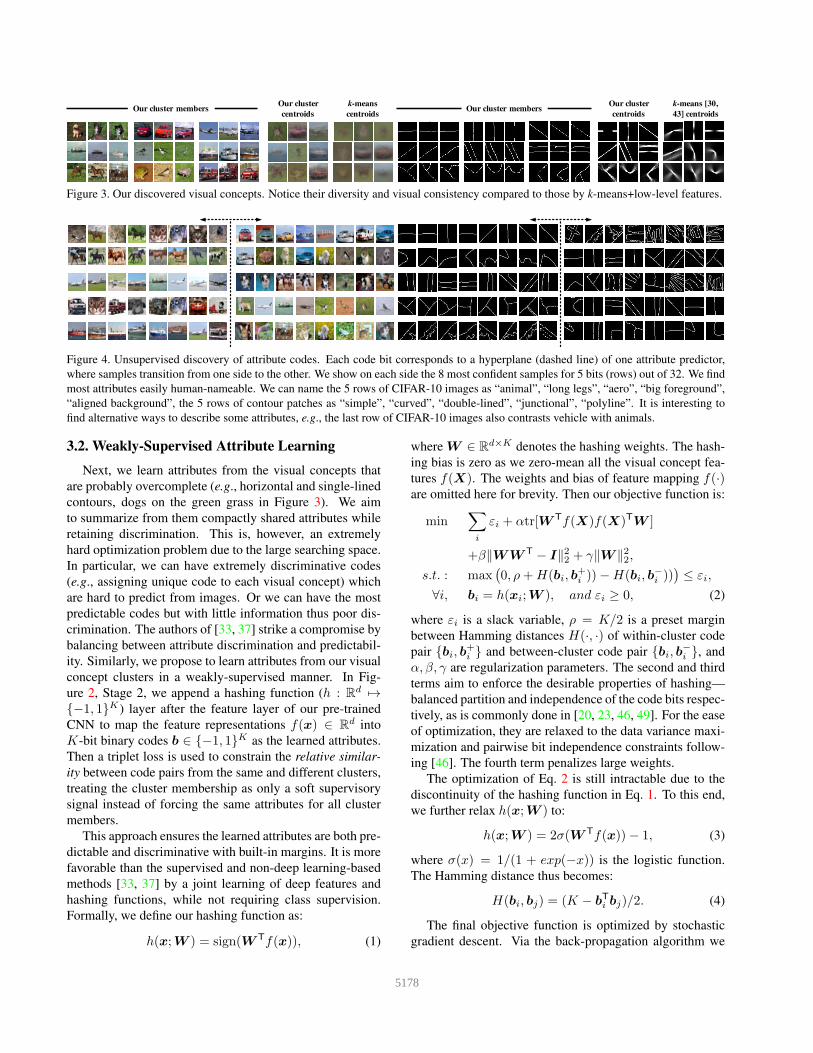
Note we initialize the clustering of color images and bi-
nary contours with HOG [9] and DAISY [50] features re-
spectively. The alternating process of clustering and CNN
feature learning usually converges within 3 rounds. Fig-
ure 3 compares our CNN clustering results with those by
k-means+initialized features. The visual concepts discov-
ered by our approach are representative, meaningful and di-
verse. They are more consistent and convey richer informa-
tion than k-means.
5177
Our cluster membersOur cluster
centroids
k-means
centroids
k-means [30,
43] centroids
Our cluster
centroidsOur cluster members
Figure 3. Our discovered visual concepts. Notice their diversity and visual consistency compared to those by k-means+low-level features.
Figure 4. Unsupervised discovery of attribute codes. Each code bit corresponds to a hyperplane (dashed line) of one attribute predictor,
where samples transition from one side to the other. We show on each side the 8 most confident samples for 5 bits (rows) out of 32. We find
most attributes easily human-nameable. We can name the 5 rows of CIFAR-10 images as “animal”, “long legs”, “aero”, “big foreground”,
“aligned background”, the 5 rows of contour patches as “simple”, “curved”, “double-lined”, “junctional”, “polyline”. It is interesting to
find alternative ways to describe some attributes, e.g., the last row of CIFAR-10 images also contrasts vehicle with animals.
3.2. WeaklySupervised Attribute Learning
Next, we learn attributes from the visual concepts that
are probably overcomplete (e.g., horizontal and single-lined
contours, dogs on the green grass in Figure 3). We aim
to summarize from them compactly shared attributes while
retaining discrimination. This is, however, an extremely
hard optimization problem due to the large searching space.
In particular, we can have extremely discriminative codes
(e.g., assigning unique code to each visual concept) which
are hard to predict from images. Or we can have the most
predictable codes but with little information thus poor dis-
crimination. The authors of [33, 37] strike a compromise by
balancing between attribute discrimination and predictabil-
ity. Similarly, we propose to learn attributes from our visual
concept clusters in a weakly-supervised manner. In Fig-
ure 2, Stage 2, we append a hashing function (h : Rd 7→{−1, 1}K) layer after the feature layer of our pre-trained
CNN to map the feature representations f(x) ∈ Rd into
K-bit binary codes b ∈ {−1, 1}K as the learned attributes.
Then a triplet loss is used to constrain the relative similar-
ity between code pairs from the same and different clusters,
treating the cluster membership as only a soft supervisory
signal instead of forcing the same attributes for all cluster
members.
This approach ensures the learned attributes are both pre-
dictable and discriminative with built-in margins. It is more
favorable than the supervised and non-deep learning-based
methods [33, 37] by a joint learning of deep features and
hashing functions, while not requiring class supervision.
Formally, we define our hashing function as:
h(x;W ) = sign(W Tf(x)), (1)
where W ∈ Rd×K denotes the hashing weights. The hash-
ing bias is zero as we zero-mean all the visual concept fea-
tures f(X). The weights and bias of feature mapping f(·)are omitted here for brevity. Then our objective function is:
min∑
i
εi + αtr[W Tf(X)f(X)TW ]
+β‖WWT − I‖22 + γ‖W ‖22,
s.t. : max(
0, ρ+H(bi, b+
i ))−H(bi, b−
i )))
≤ εi,
∀i, bi = h(xi;W ), and εi ≥ 0, (2)
where εi is a slack variable, ρ = K/2 is a preset margin
between Hamming distances H(·, ·) of within-cluster code
pair {bi, b+
i } and between-cluster code pair {bi, b−
i }, and
α, β, γ are regularization parameters. The second and third
terms aim to enforce the desirable properties of hashing—
balanced partition and independence of the code bits respec-
tively, as is commonly done in [20, 23, 46, 49]. For the ease
of optimization, they are relaxed to the data variance maxi-
mization and pairwise bit independence constraints follow-
ing [46]. The fourth term penalizes large weights.
The optimization of Eq. 2 is still intractable due to the
discontinuity of the hashing function in Eq. 1. To this end,
we further relax h(x;W ) to:
h(x;W ) = 2σ(W Tf(x))− 1, (3)
where σ(x) = 1/(1 + exp(−x)) is the logistic function.
The Hamming distance thus becomes:
H(bi, bj) = (K − bT
i bj)/2. (4)
The final objective function is optimized by stochastic
gradient descent. Via the back-propagation algorithm we
5178

fine-tune our CNN to update both the feature representa-
tions f(·) and hashing functions h(·). In practice, we ini-
tialize W as the projection computed by [37] on low-level
features. During CNN tuning, data xi is randomly sampled
from all the clusters, x+
i is randomly drawn from the same
cluster, while x−
i is chosen as the between-cluster one that
most violates the triplet ranking order (loss is maximum)
in one random mini-batch. We still need to decide K, the
number of attribute codes we wish to learn. However, there
is no clue to predict a priori which codes will be useful,
so we leave it to experimental evaluation. We show that
the learned attribute codes via our approach highly corre-
late with a variety of semantic concepts, although we do
not explicitly enforce the learning to be semantic. Figure 4
show examples of attribute codes learned from images and
contours, e.g., “animals” at various backgrounds, “simple”
contours full of various single-lined ones etc. This vali-
dates that we are indeed capable of extracting meaningful
attributes shared across visual clusters.
4. Applications
4.1. Object Detection Pretraining
We first evaluate the quality of our feature representa-
tions under the proposed unsupervised learning paradigm.
We choose to fine-tune our learned features for another task
of object detection on PASCAL VOC 2007 to examine the
feature transferability, treating our unsupervised attribute
learning as a pre-training step. To acquire a deeper under-
standing of image contents and learn more effective feature
representations, we train our unsupervised model this time
on the large-scale ImageNet 2012 training set [10]. It con-
tains 1.3 million images (labels discarded), much more than
that in CIFAR-10, and has larger image diversity. But it is
more challenging to perform unsupervised learning on the
high-resolution ImageNet images than on the 32× 32 pixel
CIFAR-10 images and 45 × 45 BSDS500 contour patches,
since the pixel variety grows exponentially with spatial res-
olution. Then following [12], we sidestep this challenge by
learning from sampled patches at resolution 96× 96.
We use the AlexNet-style architecture as in [12] for un-
supervised pre-training, but adjust it to the Fast R-CNN
framework [21] for fast detection on the input image of size
227×227. For pre-training on ImageNet, we particulary ini-
tialize our first clustering step with the more elaborated fea-
tures (SIFT+color Fisher Vectors) in [36] in this harder case,
and form 30 thousand concept clusters. For fine-tuning on
the VOC training set, we copy our pre-trained weights up
to the conv5 layer and initialize the fully connected layers
with Gaussian random weights.
4.2. Image Retrieval and Classification
Image retrieval on CIFAR-10 dataset: Figures 1 and 4
already show that our attributes can describe meaningful
image properties learned from the CIFAR-10 dataset. Al-
though they do not have explicit names, many of them
strongly correspond to semantics and even convey high-
level category information. This makes them suitable to
be used as binary hash codes for fast and effective image
retrieval.
Image classification on STL-10 and Caltech-101 dataset:
To classify the high-resolution images from STL-10 (96 ×96) and Caltech-101 (roughly 300×200), we follow [13] to
unsupervisedly train CNN on the 32× 32 patches extracted
from STL-10 images. For an arbitrarily sized test image, we
compute all the convolutional responses and apply the pool-
ing method to the feature maps of each layer: 4-quadrant
max-pooling for STL-10, and 3-layer spatial pyramid for
Caltech-101. Finally, one-vs-all SVM classifiers are trained
on the pooled features. Here we use our learned features
again to validate their semantic quality for classification,
which enables a fair comparison with [13] as well.
4.3. Contour Detection
The attributes of image contours are little explored.
Here we argue that such mid-level attributes other than the
commonly-used low-level features (e.g., DAISY [50]) are
very valuable to detect image contours or even their en-
closed objects. We show the value of our unsupervised at-
tribute learning method in the task of contour detection. We
are aware of only two related works [30, 43] that unsuper-
visedly learn “sketch tokens” by k-means for contour detec-
tion. While their results are satisfying, “sketch tokens” can
be at most seen as the instances of a single-attribute about
contour shape.
Recall that we previously have only learned unsuper-
vised contour attributes from the binary contour patches—
hand drawn sketches of natural images. One question re-
mains unaddressed: how to predict for an input color im-
age the contours and associated attributes simultaneously?
We propose an efficient framework as shown in Figure 5 to
achieve this goal. We first train an initial CNN model to dis-
tinguish between the one million 45× 45 color patches cor-
responding to contours and one million non-contour 45×45patches from BSDS500 dataset. This binary task teaches
CNN to learn preliminary features and to classify whether
the central point of a given color patch is an edge or not,
without taking care of the patch attributes. Such simplifica-
tion usually produces contour predictions with high recall
but many false positives. Then we leverage the contour at-
tributes to refine the pre-trained CNN in a multi-label pre-
diction task. We employ a target of K+1 labels, all normal-
ized to {0, 1} and consisting of one binary edge label and
the K-bit attributes previously learned from the correspond-
ing binary edge patch. The attribute codes for non-edge
patches are treated as missing labels, of which the gradients
are not back-propagated to update CNN weights.
5179

...
CNN Two-waysoftmax loss
Feature layer
Edge or non-edge point?
CNN Feature layer
K-bit binary attribute codes
1-bit binary edge label
ofCross
entropyloss
Figure 5. Two-step framework for predicting contours and contour
attributes from natural image patches: binary edge classification
followed by multi-label prediction. The CNNs have shared archi-
tectures and weights.
Figure 6. Patch-wise edge map prediction. We use the thresholded
K = 16-bit attributes (we only show 3 in red dots) as hash codes
to retrieve the contour patches (red box) from training data.
Given a converged network, the final prediction is made
by directly passing the entire image through the convolu-
tional and pooling layers, and generating K+1-length vec-
tors via the fully connected layers at different spatial loca-
tions. This is more efficient than predicting for individual
patches due to the shared feature computation. As a result,
we obtain one edge map and K attribute maps which are of
the same size with input but not thresholded (i.e., intensity
maps). Note that such an edge map is pixel-wise and may be
noisy and inconsistent in local regions. Therefore, we also
make a robust patch-wise prediction using the thresholded
attribute vector (K-length) for each patch as hash codes,
and find its Hamming nearest neighbor from training data.
We simply transfer the neighboring contour patches to the
output and average all the overlapping patches as in [19],
followed by non-maximum suppression. Figure 6 illustrates
an example of such patch-wise prediction.
5. Results
Datasets and evaluation metrics: For object detection, we
follow the standard Fast R-CNN evaluation pipeline [21]
on the PASCAL VOC 2007 [15] test set, which consists of
4952 images with 20 object categories. No bounding box
regression is used. The average precision (AP) and mAP
measures are reported.
For image retrieval, we use the CIFAR-10 dataset [26]
that contains 60000 color images in 10 classes. We follow
the standard protocol of using 50000 training and 10000
testing images to unsupervisedly learn visual attributes.
During the retrieval phase, we randomly sample 1000 im-
ages (100 per class) as the query, and use the remaining
images as the gallery set as in [14]. The evaluation metrics
are mAP and precision at N samples. The average of 10
experimental results is reported.
For image classification, the 100 thousand unlabeled im-
ages of STL-10 [8] are used for our unsupervised attribute
learning. Later, on STL-10 the SVM is trained on 10 pre-
defined folds of 500 training images per class, an we report
the mean and standard deviation of classification results on
the 800 test images per class. On Caltech-101 [17] we fol-
low [13] to select 30 random samples per class for training
and no more than 50 samples per class for testing (images
are resized to 150 × 150 pixels), and repeat the procedure
10 times to report the mean and standard deviation again.
For contour detection, we use the BSDS500 dataset [2]
with 200 training, 100 validation and 200 testing images.
We evaluate by: fixed contour threshold (ODS), per-image
best threshold (OIS), and average precision (AP) [2].
Implementation details: Throughout this paper, we set αand β in Eq. 2 to 1, γ to 0.0005, and we use linear SVM
classifiers with C = 0.1. For object detection pre-training,
we adopt the AlexNet-style architecture [12]. The unsuper-
vised network training converges in about 200K iterations,
3.5 days on a K40 GPU. We start with an initial learning
rate of 0.001, and reduce it by a factor of 10 at every 50K it-
erations. We use the momentum of 0.9, and mini-batches of
256 resized images. For image retrieval and classification,
we use the architectures of [14] (3 layers) and [13] (4 lay-
ers: 92c5-256c5-512c5-1024f), respectively. We generally
follow their training details. For contour detection, We use
the 6-layer CNN architecture of [43]. The momentum is set
to 0.9, and mini-batch size to 64 patches. The initial learn-
ing rate is 0.01, and decreased by a factor of 10 every 40K
iterations until the maximum iteration 150K is reached.
5.1. Object Detection Pretraining
Quality evaluation of unsupervised pre-training: Before
transferring our pre-trained features to object detection, we
first directly evaluate the quality of our unsupervised pre-
training on the ImageNet dataset, which is a perfect testbed
due to its large size and rich data diversity. We consider
evaluating our discovered visual clusters and attributes, the
two key outputs from our unsupervised training.
Figure 3 provides some qualitative clustering results on
relatively simple datasets. Now we quantify the clustering
effects on ImageNet given the formed 30 thousand clusters
and 1 thousand ground truth classes (not used during clus-
tering). Specifically, the cluster purity is calculated as to
correspond to the percentage of cluster members with the
5180

Table 1. Detection results (%) with Fast R-CNN on the test set of PASCAL VOC 2007. We directly add our results to those reported in [34].
The results of [12] and [47] read different to their original evaluations because they use the framework of Fast R-CNN here instead of R-
CNN [22]. The R-CNN results of [12] are included as a reference. Our features pre-trained by unsupervised attribute learning (K = 32, 64
bits) produce closer results to that of the recent unsupervised features [34] and supervised features pre-trained on ImageNet with labels.Method aero bike bird boat bottle bus car cat chair cow table dog horse mbike person plant sheep sofa train tv mAP
[12] by R-CNN 60.5 66.5 29.6 28.5 26.3 56.1 70.4 44.8 24.6 45.5 45.4 35.1 52.2 60.2 50.0 28.1 46.7 42.6 54.8 58.6 46.3
Doersch et al. [12] 54.4 50.8 30.1 28.9 10.3 57.5 60.8 46.3 19.8 38.5 51.5 37.4 60.6 53.0 45.1 14.2 26.0 44.5 55.6 43.7 41.4
Wang and Gupta [47] 53.9 53.9 30.5 29.6 10.8 56.0 59.0 46.1 19.6 45.7 43.9 41.6 65.6 58.6 48.2 17.4 34.8 41.2 64.5 46.5 43.3
Ours (K = 32 bits) 59.2 61.6 31.2 33.4 27 58.3 64.9 49.1 28.6 50.4 51.9 44.7 57.9 58.5 52.3 29.6 46.1 43.2 65.6 59.2 48.6
Ours (K = 64 bits) 62.6 63.7 37.6 34.9 28.77 57.6 66.2 51.6 30.7 51.5 48.5 47.1 55.6 59.8 49.2 27.5 47.8 41.4 63.6 59.7 49.3
CFN-9 (max) [34] 61.5 64.3 36.4 36.1 20.8 65.8 69.0 59.2 30.3 50.0 58.1 50.7 70.6 67.2 56.0 22.7 44.7 52.8 66.9 52.0 51.8
ImageNet [21] 65.1 70.3 53.6 41.6 25.1 69.3 68.9 68.8 30.4 63 62.3 63.3 72.7 64.5 57.1 25.2 50.6 54 70.1 55.1 56.5
Table 2. Retrieval results on the CIFAR-10 dataset: K-bit (16-64)
Hamming ranking accuracy by mAP and precision@ N = 1000.
MethedmAP (%) precision (%) @ N
16 32 64 16 32 64
SH [49] 12.55 12.42 12.56 18.83 19.72 20.16
PCAH [46] 12.91 12.60 12.10 18.89 19.35 18.73
LSH [20] 12.55 13.76 15.07 16.21 19.10 22.25
ITQ [23] 15.67 16.20 16.64 22.46 25.30 27.09
DH [14] 16.17 16.62 16.96 23.79 26.00 27.70
Ours 16.82 17.01 17.21 24.54 26.62 28.06
Query
Ours
DH [14]
ITQ [23]
LSH [20]
PCAH [46]
SH [49]
Figure 7. Top 8 images retrieved by different hashing methods in
comparison to ours (K = 64) on the CIFAR-10 dataset.
same class label. Our CNN clustering attains the value of
0.34, much higher than 0.16 by k-means clustering with
hand-crafted features [36]. This validates the proposed clus-
tering indeed discovers some level of categorical semantics,
although the purity value is not as high as that on e.g., the
less diverse CIFAR-10 dataset. This also demonstrates the
scalability of our unsupervised paradigm to large-scale data.
For our discovered unsupervised attributes, it is not easy
to either subjectively name them or compare them to the
available human labels (the ImageNet Attribute subset [39]
has ambiguous labels in itself) by consensus. We leave their
quality evaluation as future work.
Feature transferability to detection: Table 1 reports the
results of transferring pre-trained features to the VOC 07
detection task. Our unsupervised features yield higher per-
formance (49.3% mAP, K = 64) than the other unsuper-
vised ones [12, 47], and are comparable to the recent un-
supervised features [34] and supervised one with ImageNet
labels. Thus we argue that learning unsupervised visual at-
tributes helps understand image contents and objects, and
the features learned this way are semantically meaningful.
Table 3. Classification accuracies (%) of unsupervised (top cell)
and supervised (bottom cell) methods on STL-10 and Caltech-101.
Method STL-10 Caltech-101
Multi-way local pooling [6] — 77.3 ± 0.6
Slowness on videos [53] 61.0 74.6
HMP [4] 64.5 ± 1 —
Multipath HMP [5] — 82.5 ± 0.5
View-Invariant k-means [24] 63.7 —
Exemplar-CNN [13] 75.4 ± 0.3 87.2 ± 0.6
Ours (K = 16 bits) 74.9 ± 0.4 86.1 ± 0.7
Ours (K = 32 bits) 76.3 ± 0.4 87.8 ± 0.5
Ours (K = 64 bits) 76.8 ± 0.3 89.4 ± 0.5
Supervised state of the art 70.1 [45] 91.44 [25]
5.2. Image Retrieval
This experiment shows the effectiveness of the attributes
learned by our approach when they are used as binary hash
codes in a retrieval task. We compare with five related un-
supervised hashing methods in Table 2. As shown, our
method significantly outperforms traditional SH, PCAH,
LSH and ITQ methods due to the joint learning of hash-
ing functions and features. We also consistently improve
the mAP at different code bits over Deep Hashing (DH)
since we adopt a discriminative paradigm rather than a re-
constructive one.
Figure 7 visualizes our clear advantages in terms of both
retrieval accuracy and consistency. Since our approach can
discover the latent properties of both image foreground and
background in an unsupervised manner, it is better at inter-
preting image scenes using multi-source information. Usu-
ally we generate K = 64 attribute codes which takes about
10ms on GPU. The code retrieval time is negligible.
5.3. Image Classification
For the STL-10 and Caltech-101 images, we learn vi-
sual attributes from 32 × 32 patches and use the resulting
features to classify. Table 3 studies whether such patch-
level learning will give rise to class discrimination at im-
age level. We observe that our features trained with rich
attributes lead to higher classification accuracies (peak at
K = 64) on both datasets than all the other unsupervised
features, and even out-compete the supervised one [45] by
6.7% on STL-10. This suggests that resolving attribute con-
fusions indeed leads to class-discriminating features, even
in the patch space. Moreover, the larger gains here than
5181

Table 4. Contour detection results on BSDS500. The top and bot-
tom cells list the pixel-wise and patch-wise methods, respectively.
Method ODS OIS AP
Sketch Token [30] 0.73 0.75 0.78
Ours (pixel) 0.75 0.77 0.79
N4-Fields [19] 0.75 0.77 0.78
DeepContour [43] 0.76 0.77 0.80
Ours (patch, K = 8 bits) 0.74 0.75 0.77
Ours (patch, K = 16 bits) 0.77 0.78 0.82
Ours (patch, K = 32 bits) 0.77 0.78 0.81
Figure 8. Contour detection examples on BSDS500: (from left to
right) original image, results of Sketch Token [30], our pixel-wise
method, DeepContour [43], and our patch-wise method (K = 16).
those on the simple CIFAR-10 dataset show our potential to
learn from more complex and diverse image data in the real
world.
5.4. Contour Detection
Table 4 compares our pixel-wise and patch-wise contour
detection methods with related methods. Since our con-
tour pixels are jointly learned and output with rich contour
attributes, our pixel-wise prediction tends to focus more
on distinctive meaningful edges. The gains over k-means-
based “shape-only” learner [30] validate this point, and
their visual differences are shown in Figure 8. Our patch-
wise version largely eliminates the pixel noise by averag-
ing nearest neighbor patches retrieved using the attribute
codes, with better results than the similar methods of deep
neighbor searching [19] and clustering-based deep classifi-
cation [43]. This proves our learned attributes can provide
more faithful mid-level cues about image contours (see the
detailed structures in our patch-wise edge map in Figure 8).
We observe saturated performance when using K = 16attribute bits for retrieving contour patch neighbors. Note
that neighbor retrieval in Hamming space is costless. We
only need to enumerate the binary attribute codes with no
searching at all. So to produce the final edge map, nearly
all the time is spent on generating the required K + 1 maps
themselves. The whole procedure takes about 60ms for a
321× 481 image on a GPU.
Table 5. Ablation tests of image retrieval (mAP %) on CIFAR-10
and classification (accuracy %) on STL-10 and Caltech-101. All
baselines work on K = 64 and we compare with the alternative
clustering (middle cell) and hashing (bottom cell) techniques.
Algorithm CIFAR-10 STL-10 Caltech-101
Our original method 17.21 76.8 ± 0.3 89.4 ± 0.5
k-means+CNN 17.16 76.2 ± 0.3 88.6 ± 0.5
k-means+HOG 16.94 75.5 ± 0.3 87.3 ± 0.6
Triplet hashing [27] 17.17 76.7 ± 0.4 88.8 ± 0.6
UTH [31] 17.02 74.9 ± 0.4 86.7 ± 0.6
DH [14] 17.05 75.6 ± 0.3 87.9± 0.6
5.5. Ablation Tests
We finally study the key components of our approach—
unsupervised feature learning from visual clusters and
weakly-supervised hash learning to highlight their unique
strengths. At each time we replace one component with an
alternative method and report the result in Table 5.
By comparing with the performance of k-means+CNN
feature learning, we can find the benefit of using our modi-
fied unsupervised discriminative clustering method to guide
the feature learning. We observe a further performance drop
when replacing the alternating CNN feature learning with
only HOG features. In this case, less meaningful visual
clusters and features can be learned from data.
For our hashing component, we first indicate the impor-
tance of learning discriminative hashing functions by com-
paring with the unsupervised Deep Hashing (DH) [14]. DH
only hashes to reconstruct the latent features thus yielding
much less discriminative results. In contrast, our weakly-
supervised method samples hash code triplets to softly en-
force the cluster discrimination. Our method outperforms
the similar triplet hashing methods [27, 31], mainly because
they lack the hash code constraints (in Eq. 2) and define
triplets by the noisy raw feature similarity respectively.
6. Conclusion
This paper proposes an unsupervised approach to deep
learning discriminative attributes from unlabeled data. The
input of our system can be natural images (patches) or
binary contour patches. The output is a compact list of
attributes in the form of binary codes. This is achieved
by a novel two-stage pipeline consisting of unsupervised
discriminative clustering and weakly-supervised hashing,
where the visual clusters, hashing functions and feature rep-
resentations are jointly learned. The resulting visual at-
tributes and features are found to capture strong semantic
meanings, and are transferrable to several important vision
tasks. The transferability to more tasks will be studied in
the future.
Acknowledgment. This work is partially supported by
SenseTime Group Limited and the General Research Fund
sponsored by the Research Grants Council of the Kong
Kong SAR (CUHK 416713).
5182

References
[1] A.Dosovitskiy, J.T.Springenberg, M.Riedmiller, and T.Brox.
Discriminative unsupervised feature learning with convolu-
tional neural networks. In NIPS, 2014.
[2] P. Arbelaez, M. Maire, C. Fowlkes, and J. Malik. Con-
tour detection and hierarchical image segmentation. TPAMI,
33(5):898–916, 2011.
[3] T. L. Berg, A. C. Berg, and J. Shih. Automatic attribute dis-
covery and characterization from noisy web data. In ECCV,
2010.
[4] L. Bo, X. Ren, and D. Fox. Unsupervised feature learning
for RGB-D based object recognition. In ISER, 2012.
[5] L. Bo, X. Ren, and D. Fox. Multipath sparse coding using
hierarchical matching pursuit. In CVPR, 2013.
[6] Y.-L. Boureau, N. Le Roux, F. Bach, J. Ponce, and Y. LeCun.
Ask the locals: Multi-way local pooling for image recogni-
tion. In ICCV, 2011.
[7] S. Branson, C. Wah, F. Schroff, B. Babenko, P. Welinder,
P. Perona, and S. Belongie. Visual recognition with humans
in the loop. In ECCV, 2010.
[8] A. Coates, A. Y. Ng, and H. Lee. An analysis of single-
layer networks in unsupervised feature learning. In AISTATS,
2011.
[9] N. Dalal and B. Triggs. Histograms of oriented gradients for
human detection. In CVPR, 2005.
[10] J. Deng, W. Dong, R. Socher, L. J. Li, K. Li, and L. Fei-
Fei. Imagenet: A large-scale hierarchical image database. In
CVPR, 2009.
[11] C. Doersch, A. Gupta, and A. A. Efros. Mid-level visual
element discovery as discriminative mode seeking. In NIPS,
2013.
[12] C. Doersch, A. Gupta, and A. A. Efros. Unsupervised vi-
sual representation learning by context prediction. In ICCV,
2015.
[13] A. Dosovitskiy, P. Fischer, J. T. Springenberg, M. Ried-
miller, and T. Brox. Discriminative unsupervised feature
learning with exemplar convolutional neural networks. arXiv
preprint, arXiv:1406.6909v2, 2015.
[14] V. Erin Liong, J. Lu, G. Wang, P. Moulin, and J. Zhou. Deep
hashing for compact binary codes learning. In CVPR, 2015.
[15] M. Everingham, L. Van Gool, C. Williams, J. Winn, and
A. Zisserman. The pascal visual object classes (VOC) chal-
lenge. IJCV, 88(2):303–338, 2010.
[16] A. Farhadi, I. Endres, D. Hoiem, and D. Forsyth. Describing
objects by their attributes. In CVPR, 2009.
[17] L. Fei-Fei, R. Fergus, and P. Perona. Learning generative
visual models from few training examples: An incremen-
tal bayesian approach tested on 101 object categories. In
CVPRW, 2004.
[18] Y. Fu, T. M. Hospedales, T. Xiang, and S. Gong. Learning
multimodal latent attributes. TPAMI, 36(2):303–316, 2014.
[19] Y. Ganin and V. S. Lempitsky. N4-fields: Neural network
nearest neighbor fields for image transforms. In ACCV, 2014.
[20] A. Gionis, P. Indyk, and R. Motwani. Similarity search in
high dimensions via hashing. In VLDB, 1999.
[21] R. Girshick. Fast R-CNN. In ICCV, 2015.
[22] R. Girshick, J. Donahue, T. Darrell, and J. Malik. Rich fea-
ture hierarchies for accurate object detection and semantic
segmentation. In CVPR, 2014.
[23] Y. Gong and S. Lazebnik. Iterative quantization: A pro-
crustean approach to learning binary codes. In CVPR, 2011.
[24] K. Y. Hui. Direct modeling of complex invariances for visual
object features. In ICML, 2013.
[25] H. Kaiming, Z. Xiangyu, R. Shaoqing, and J. Sun. Spatial
pyramid pooling in deep convolutional networks for visual
recognition. In ECCV, 2014.
[26] A. Krizhevsky. Learning multiple layers of features from
tiny images. Technical report, University of Toronto, 2009.
[27] H. Lai, Y. Pan, and S. Yan. Simultaneous feature learning
and hash coding with deep neural networks. In CVPR, 2015.
[28] C. Lampert, H. Nickisch, and S. Harmeling. Learning to de-
tect unseen object classes by between-class attribute transfer.
In CVPR, 2009.
[29] Y. Li, L. Liu, C. Shen, and A. van den Hengel. Mid-level
deep pattern mining. In CVPR, 2015.
[30] J. Lim, C. L. Zitnick, and P. Dollar. Sketch tokens: A learned
mid-level representation for contour and object detection. In
CVPR, 2013.
[31] J. Lin, O. Morere, J. Petta, V. Chandrasekhar, and A. Veil-
lard. Tiny descriptors for image retrieval with unsupervised
triplet hashing. arXiv preprint, arXiv:1511.03055v1, 2015.
[32] J. Liu, B. Kuipers, and S. Savarese. Recognizing human ac-
tions by attributes. In CVPR, 2011.
[33] S. Ma, S. Sclaroff, and N. Ikizler-Cinbis. Unsupervised
learning of discriminative relative visual attributes. In EC-
CVW, 2012.
[34] M. Noroozi and P. Favaro. Unsupervised learning of visual
representations by solving jigsaw puzzles. arXiv preprint,
arXiv:1603.09246, 2016.
[35] D. Parikh and K. Grauman. Interactively building a discrim-
inative vocabulary of nameable attributes. In CVPR, 2011.
[36] F. Perronnin and J. Sanchez. Compressed fisher vectors for
large scale visual recognition. In ICCVW, 2011.
[37] M. Rastegari, A. Farhadi, and D. Forsyth. Attribute discov-
ery via predictable discriminative binary codes. In ECCV,
2012.
[38] M. Rohrbach, M. Stark, G. Szarvas, I. Gurevych, and
B. Schiele. What helps where – and why? semantic relat-
edness for knowledge transfer. In CVPR, 2010.
[39] O. Russakovsky and L. Fei-Fei. Attribute learning in large-
scale datasets. In ECCVW, 2010.
[40] R. Salakhutdinov and G. Hinton. Semantic hashing. Int. J.
Approx. Reasoning, 50(7):969–978, 2009.
[41] S. Shankar, V. K. Garg, and R. Cipolla. Deep carving: Dis-
covering visual attributes by carving deep neural nets. In
CVPR, 2015.
[42] S. Shankar, J. Lasenby, and R. Cipolla. Semantic transform:
Weakly supervised semantic inference for relating visual at-
tributes. In ICCV, 2013.
[43] W. Shen, X. Wang, Y. Wang, X. Bai, and Z. Zhang. Deep-
contour: A deep convolutional feature learned by positive-
sharing loss for contour detection. In CVPR, 2015.
5183

[44] S. Singh, A. Gupta, and A. A. Efros. Unsupervised discovery
of mid-level discriminative patches. In ECCV, 2012.
[45] K. Swersky, J. Snoek, and R. P. Adams. Multi-task bayesian
optimization. In NIPS, 2013.
[46] J. Wang, S. Kumar, and S.-F. Chang. Semi-supervised hash-
ing for scalable image retrieval. In CVPR, 2010.
[47] X. Wang and A. Gupta. Unsupervised learning of visual rep-
resentations using videos. In ICCV, 2015.
[48] Y. Wang and G. Mori. A discriminative latent model of ob-
ject classes and attributes. In ECCV, 2010.
[49] Y. Weiss, A. Torralba, and R. Fergus. Spectral hashing. In
NIPS, 2009.
[50] S. Winder, G. Hua, and M. Brown. Picking the best DAISY.
In CVPR, 2009.
[51] R. Xia, Y. Pan, H. Lai, C. Liu, and S. Yan. Supervised hash-
ing for image retrieval via image representation learning. In
AAAI, 2014.
[52] F. Zhao, Y. Huang, L. Wang, and T. Tan. Deep semantic rank-
ing based hashing for multi-label image retrieval. In CVPR,
2015.
[53] W. Zou, S. Zhu, K. Yu, and A. Y. Ng. Deep learning of
invariant features via simulated fixations in video. In NIPS,
2012.
5184
Recommended