Unprofitable Affiliates and Income Shifting Behavior
Lisa De Simone
Stanford Graduate School of Business
Kenneth J. Klassen
University of Waterloo
Jeri K. Seidman
University of Texas at Austin
August 2014
Income shifting from high-tax to low-tax jurisdictions is commonly considered as a primary
method of reducing worldwide tax burdens of multinational firms. Extant research generally
makes the high- and low-tax distinctions using statutory or aggregated effective tax rates.
However, current losses also affect the marginal tax rates of affiliates. In the absence of
carryback or carryforward provisions, an unprofitable affiliate has a marginal tax rate of zero.
Thus, an unprofitable affiliate can temporarily alter the income shifting incentives and strategy of
a multinational firm. We alter prior estimation approaches to allow for the inclusion of loss
affiliates and test whether the unexplained income of unprofitable affiliates and their associated
profitable affiliates is correlated with tax-related factors. Results suggest that multinational firms
with an unprofitable affiliate use tax-motivated shift-to-loss transfer pricing strategies.
Keywords: transfer pricing, income shifting, losses
______________________________________________________________________________
The authors appreciate helpful discussions with Jennifer Blouin and Leslie Robinson, as well as
comments from Mary Barth, Daniel Collins, Cristi Gleason, Jost Heckemeyer, Daniel Lynch, Ed
Maydew, Edmund Outslay, Kathy Petroni, Richard Sansing, Casey Schwab, Bridget Stomberg,
Erin Towery, Benjamin Whipple, and workshop participants at Michigan State University, the
University of Georgia, the University of Iowa, the Stanford Graduate School of Business, the
EIASM 4th
Workshop on Current Research in Taxation, the Tax Policy and the Activities of
Multinational Firms Conference at Eberhard Karls Universität Tübingen, and the 2014 Stanford
Accounting Summer Camp. The authors are thankful for financial support from the McCombs
Research Excellence Fund and the McCombs Supply Chain Management Center of Excellence.

1
1. INTRODUCTION
The accounting, finance, and economics literatures investigate income tax reduction
through cross-border income shifting. Prior research finds that firms undertake a strategy of
shifting income out of high-tax jurisdictions into low-tax jurisdictions, thus reporting lower
profit in high-tax affiliates and higher profit in low-tax affiliates.1 In a multinational firm with
only profitable affiliates, this shifting strategy results in tax savings equal to the dollars of
income shifted times the rate differential between the high-tax and low-tax affiliates, net of any
costs.
Prior research generally determines relative tax rate groupings using either the statutory
tax rate of the jurisdiction or an aggregated effective tax rate. These methods mask an alternative
tax-saving recipient of shifted income: an unprofitable affiliate. Ignoring the potential benefit of
a loss carryback or carryforward, an unprofitable affiliate becomes an extremely low-tax affiliate
because it has a marginal tax rate of zero. A firm may shift income from a profitable affiliate into
an unprofitable affiliate, reporting lower profit in the profitable affiliate and a smaller loss in the
unprofitable affiliate. Thus, shifting income into unprofitable affiliates often results in higher tax
savings than the “traditional” transfer pricing strategy because the savings are equal to the dollars
of income shifted times the rate of the profitable affiliate.
However, this alternative shift-to-loss strategy is not costless. Efficient transfer pricing
strategies can be expensive to put in place and, for this reason, are often set over a multi-year
period. In contrast, affiliate losses are relatively transitory as the affiliate will either return to
profitability or cease operations.2 Adjusting the income shifting regime to take advantage of an
1 See for example, Collins, Kemsley and Lang (1998); Klassen, Lang and Wolfson (1993); Desai and Dharmapala
(2006); Huizinga and Laeven (2008); Weichenrieder (2009); Klasssen and Laplante (2012); Dharmapala and Riedel
(2013); Dharmapala (2014); and Dyreng and Markle (2014). 2 It is possible for a multinational to continue to operate an affiliate with structural losses due to strategic or other
reasons. In general, however, one would expect this to be rare.

2
unprofitable affiliate may necessitate costly tax planning, such as re-characterizing the nature of
significant transactions or reorganizing the global supply chain structure. Each of these requires
creation of supporting documentation, procurement of additional professional services/advice,
and/or a reduction in the probability of sustaining a position upon audit. Whether the tax savings
from using an unprofitable affiliate as an alternative recipient of shifted income outweigh the
adjustment costs necessary to change from the traditional strategy is an empirical question,
especially if losses are expected to be transitory or unexpectedly arise in an affiliate.
Our paper uses affiliate-level data on multinational firms to explore responses to the
income shifting incentives generated by unprofitable affiliates. We follow Claessens and Laeven
(2004) and measure profitability as return on assets plus one, which allows us to include
unprofitable affiliates in the traditional logged Cobb Douglas profit prediction model. On a
sample that includes both profitable and unprofitable affiliates, we estimate a model which
specifies affiliate profitability as a function of labor; assets; productivity; macroeconomic,
industry-level, and firm-level shocks; and tax-related factors.
We study whether the unexplained profitability of affiliates varies with tax factors related
to the shift-to-loss strategy, such as the adjustment costs and the potential tax savings of such a
strategy. Results show that the profit of unprofitable affiliates is due at least in part to tax-
motivated shift-to-loss behavior. We document that the statutory tax rate of unprofitable
affiliates affects the unexplained profit of both unprofitable affiliates and their associated
profitable affiliates. Consistent with prior literature using profitable affiliates, we estimate that a
one standard deviation increase in the statutory tax rate of profitable affiliates is associated with
a 4.8 percentage decrease in profitability reported by the average profitable affiliate. In contrast,
we estimate that a one standard deviation increase in the statutory tax rate of unprofitable
affiliates is associated with a 6.6 percent increase in profitability reported by the average

3
unprofitable affiliate, and a 3.9 percent decrease in the profitability reported by the average
profitable affiliate. We also provide evidence that suggests that corporate taxpayers respond to
transfer pricing risk and jurisdictional scrutiny of reported losses, and that the profit shifted by
profitable affiliates to their unprofitable affiliates is proportional to their relative economic
activity. Overall, our study provides evidence that shifting income to an unprofitable affiliate is
an important transfer pricing consideration for multinational firms.
This paper is in the spirit of Gramlich, Limpaphayom, and Rhee (2004) (hereafter GLR)
and Onji and Vera (2010), who both study income shifting among keiretsu members in Japan.
Both papers document a lower incidence of losses in affiliated members relative to unaffiliated
members. These results suggest that affiliated groups band together to save keiretsu-level income
taxes by shifting taxable profit into unprofitable members.3 We contribute to this stream of
research by using a cross-border setting to test whether the unexplained profit reported by
unprofitable affiliates varies with the expected benefits, costs and risks of a shift-to-loss strategy.
The cross-border setting allows us to exploit variation in tax rates and heterogeneous affiliate tax
characteristics. Importantly, we are the first to use a cross-border sample in tests of tax-motivated
shift-to-loss income shifting and thus are the first to document that the presence of loss affiliates
affects the unexplained profitability of affiliated firms.
This study informs policy makers and public economists who, in light of increased
multinational income shifting and the recent economic downturn, are debating how to curb tax
base erosion and profit shifting (Saint-Amans and Russo, 2013). By focusing on temporary
changes to the multinational corporation’s income shifting incentives, our research provides
3 This result is also consistent with risk sharing to the extent the risk sharing manifests in profitable affiliates shifting
income into unprofitable affiliates rather than profitable affiliates tolerating the losses of unprofitable affiliates. Kim
and Yi (2006) provide evidence of earnings management in affiliated Korean firms (“chaebols”), which is consistent
with risk-sharing-motivated income shifting.

4
valuable insight into the costs of temporarily altering transfer prices and the size of inframarginal
effects induced by larger tax rate changes. Our evidence that firms will respond to temporary tax-
minimizing opportunities contributes to policy maker analyses of altering tax policies targeted at
multinational corporations, such as repatriation tax holidays, temporary tax incentives for foreign
direct investors, or patent boxes.
Our results also inform policy makers regarding the semi-elasticity of reported income
with respect to changes in statutory tax rates. Our paper suggests that, by using samples of
profitable affiliates only, previous estimates of the magnitudes of income shifting in response to
tax rate changes should be considered a lower bound. Some shifting by profitable affiliates goes
to unprofitable affiliates, rather than to low-tax profitable affiliates, and by omitting this sample
of unprofitable affiliates, the estimates include the muted effect to tax rate changes for these
affiliates. In addition, our analysis is helpful for policy analyses that involve large changes or
differences in statutory tax rates, and our estimates for unprofitable affiliates provide a lower
bound of the effect size for these analyses, as described more fully below.
This study also suggests that the jurisdictions that benefit from profit shifting and those
that are injured by profit shifting are not obvious. Although low-tax jurisdictions generally
benefit from multinational income shifting, our results suggest that low-tax jurisdictions also lose
expected tax revenues during periods of economic decline. During such periods, affiliated groups
could shift income to unprofitable affiliates instead of to affiliates located in low-tax
jurisdictions, or even shift income out of profitable affiliates located in low-tax jurisdictions into
unprofitable affiliates. Further, previous research demonstrates income shifting from high-tax
jurisdictions to low-tax jurisdictions, which suggests that high-tax revenue authorities should

5
focus their audit efforts on transactions with related parties in low-tax jurisdictions.4 Our results
suggest that revenue authorities should also be concerned about affiliates shifting income out of
their jurisdiction into unprofitable affiliates, regardless of the tax rate in the unprofitable
affiliate’s jurisdiction.
Our results also inform researchers. First, researchers should consider the impact of this
alternative tax-minimizing transfer pricing strategy in their studies of the “standard” tax-
motivated transfer pricing strategy. Many income shifting studies use aggregated affiliate profits
and losses (i.e., consolidated financial statement data), which confounds the two types of income
shifting strategies by combining a number of potentially-conflicting transfer pricing incentives.5
Other income shifting studies restrict their sample to profitable affiliates.6 The removal of
unprofitable affiliates does not fully address the concern, though, because the effect of shifting to
unprofitable affiliates is also reflected in lower profitability of profitable affiliates. Further,
estimates of tax policy changes on income shifting behavior may be understated by the exclusion
of loss affiliates from the sample. Second, our study provides evidence on the trade-offs firms
make in their transfer pricing decisions. The cost of establishing a tax-efficient supply chain
cannot be easily estimated. However, evidence regarding the expected tax benefit required to
entice firms to alter their transfer pricing to a shift-to-loss strategy provides indirect evidence on
the cost, which may be useful to researchers interested in cross-sectional variation in the use of
various income-shifting strategies. Finally, this study deepens our understanding of the income
shifting practices of multinational firms. Examining a new and economically significant income
4 For example, Collins et al. (1998), Clausing (2006, 2009), and Klassen and Laplante (2012).
5 For example, high-tax profitable affiliates have an incentive to shift income out of their jurisdictions while high-tax
unprofitable affiliates may be recipients of shifted income. Low-tax profitable affiliates are likely to receive shifted
income, but in the presence of an unprofitable affiliate, they may also shift income out to the unprofitable affiliate. 6 For example, Power and Silverstein (2007), Blouin, Robinson and Seidman (2013), De Simone (2014), Markle
(2012).

6
shifting setting helps answer the call to research in Shackelford and Shevlin (2001) to increase
our ability to explain and predict income-shifting strategies beyond mere documentation.
The paper proceeds as follows. The next section provides institutional background on
how multinationals shift income as well as an overview of the literature on both cross-border
income shifting behavior and the effect of losses on firm behavior. The third section develops
our three hypotheses. Section 4 outlines the regressions and describes the data and variables we
use to test our hypotheses. Section 5 details results and Section 6 concludes.
2. BACKGROUND AND RELATED LITERATURE
2a. Income Shifting Background
The most effective income shifting strategies employ two components in concert with
each other—an operational decision and an accounting decision. The operational decision entails
tax-efficiently structuring the firm’s global supply chain such that the affiliated parties to major
intercompany transactions are strategically located. As such, multinationals often locate high-
return assets and activities in low-tax jurisdictions and relatively low-return activities in high-tax
jurisdictions.7
Further, multinationals have incentives to choose prices for these intercompany
transactions that optimizes the worldwide tax burden of the firm; this represents the accounting
decision component. Transfer pricing guidelines for income tax reporting are established by the
OECD, and have been adopted in some form by most European countries. These regulations
prescribe that for the purposes of calculating taxable income, any intercompany prices for goods,
services and intangibles should be those that would have been realized if the parties were
7 Examples of high-return activities include the research and development of unique intangibles. Examples of low-
return activities include contract manufacturing and limited-risk distribution.

7
unrelated, known as the “arm’s length principle” (OECD, 2010). However, these arm’s length
prices can be difficult to observe, especially for services, unique intangibles, and unusual or
unfinished products (PWC, 2006). This inability to always find exact market price matches for
intercompany transactions leaves multinational entities some discretion in setting transfer prices.
Further, although many multinationals strive to appropriately price a transaction during the
course of the year, they can also make so-called “topside adjustments” to these prices after the
financial books have been closed but prior to the filing of the tax return.8 Thus, the accounting
decision for how and when to set the transfer price of an intercompany transaction is flexible and
relatively nimble when compared to the operational decision.
When a multinational firm realizes an affiliate will likely earn a loss, the multinational
has a number of options to consider. First, the affiliate could simply report the loss as earned. If
its jurisdiction allows loss carryback and it was profitable during the allowed carryback period,
the reported loss will generate an immediate refund. If its jurisdiction does not allow loss
carryback (or if it was not profitable during the allowed carryback period) but does allow loss
carryforward, the reported loss will generate tax savings in the future if the affiliate returns to
profitability. If the jurisdiction of the reported loss does not allow loss carryback or loss
carryforward, the reported loss generates no tax benefit for the multinational firm. Thus, both the
adjustment costs and the benefits are lowest under this option.
Second, the multinational firm can undertake real activities to minimize the loss at the
affiliate.9 For example, the multinational could move research and development activities to a
more profitable affiliate or, as a more extreme example, move a physical factory from one
8 Because we rely on affiliate financial statement information, we are unable to measure the impact of these topside
adjustments. However, topside adjustments bias against our tests detecting income shifting behavior. 9 We assume that the aggregate level of the multinational’s activities was optimal but that its allocation of these
activities to affiliates was not. Thus, in our setting, activities are moved rather than decreased.

8
jurisdiction to another. This option likely entails significant adjustment costs and will result in a
less tax-efficient structure in the future, assuming the unprofitable affiliate returns to
profitability.
Finally, the multinational can adjust transfer prices to minimize the reported loss.
Because transfer prices have some inherent flexibility, a multinational could potentially reduce
taxes using a traditional strategy when all affiliates are profitable, but change to a shift-to-loss
strategy when losses occur in some affiliates. This is the behavior we aim to study.
The inherent flexibility in transfer prices arises because market prices for intercompany
transactions can be difficult to observe. Firms generally construct a range of prices based on
inexact “comparables,” or companies with a similar business profile. Most countries accept any
price within the range generated using such methods, and as such, firms often choose the most
tax-favored endpoint of the range.
For example, firms with a high-tax affiliate that is purchasing services from a low-tax
affiliate will choose a price at the high end of the range to minimize profits in the relatively high-
tax jurisdiction and maximize profits in the relatively low-tax jurisdiction. If the high-tax affiliate
instead earns a loss, it has several options. First, and most commonly, the firm can choose a
transfer price at the other end of the range to minimize the reported loss. Second, the firm can
adjust its search for independent comparable transactions in order to expand the range to include
a new, more favorable endpoint. Finally, if necessary, the firm can identify risks borne by the
unprofitable affiliate that resulted in the loss (e.g., foreign currency exchange or product failure
risk), or other previously uncompensated transactions that the affiliate is party to, and
compensate the affiliate for that previously un-priced contribution. However, this last option
potentially sets a precedent for less tax-favored outcomes in profitable years.

9
2b. Related Literature
Accounting, finance, and economics literatures abound with evidence that firms reduce
income taxes by shifting taxable income from relatively higher-tax jurisdictions to lower-tax
jurisdictions. Grubert and Mutti (1991) exploit the relation between profitability and the tax rate
as a measure of income shifting and variants of their research design are often used in the
literature. For example, Klassen, Lang, and Wolfson (1993) use a similar methodology to study
changes in income shifting behavior in response to tax rate changes, while Hines and Rice (1994)
employ the research design to study the use of tax havens. The approach of Hines and Rice has
become common as a general model of multinational income shifting (Dharmapala, 2014).
Alternative methods for studying tax-motivated income shifting behavior have also been
developed. Jacob (1996) considers the volume of intrafirm trade as a measure of income shifting
flexibility and shows that tax savings are related to the volume of intrafirm trade. Clausing
(2006) finds that the price of intrafirm transactions and the trading partners’ tax rates are strongly
related in a manner consistent with tax-motivated transfer pricing. Overesch (2006) uses
intercompany accounts receivable (A/R) to indirectly measure intrafirm prices and shows that the
intercompany A/R of foreign-owned German subsidiaries with a loss carryforward is less
sensitive to the tax rate differential (between the foreign parent and the German subsidiary) than
is the intercompany A/R of foreign-owned German subsidiaries without a loss carryforward.
Bernard, Jensen, and Schott (2008) find that the prices that U.S. exporters charge arm’s-length
customers are significantly higher than the prices that they charge related-parties, and that this
price wedge is greater for goods sent to countries with lower corporate tax rates or to countries
with higher import tariffs.
While there is ample evidence of tax-motivated income shifting by multinational firms,
the literature has largely focused on the benefit of shifting income from higher-tax affiliates to

10
lower-tax affiliates and ignored the benefit of shifting income from a profitable affiliate to an
unprofitable affiliate.10
Because the presence of an unprofitable affiliate can alter the income
shifting incentives of relatively low-tax profitable affiliates, this omission may have a profound
effect on measurement of income shifting. Although Klassen, Lang, and Wolfson (1993) discuss
the difficulty in measuring the tax incentives of unprofitable firms and the potential confounding
effect losses have on tax-motivated income shifting behavior, to our knowledge, only GLR and
Onji and Vera (2010) attempt to test the effect of unprofitable affiliates.11
Both GLR and Onji and Vera (2010) find that members of Japanese keiretsu groups
(member firms) appear to alter their transfer pricing behaviors in the presence of loss members.
Although these results support loss-related income shifting, their data sets do not allow the
variation in tax rates necessary to directly study the relation between tax rates and profitability.
Further, the costs and benefits of shifting income between keiretsu members will differ from
those associated with foreign affiliates in a commonly-controlled group.
While the tax-motivated income shifting literature has largely ignored the impact of
losses on cross-jurisdictional income shifting, the effect of losses on other types of tax
minimizing behavior has been studied. For example, Mackie-Mason (1990) finds that firms with
loss carryforwards are significantly less likely to issue debt than firms without loss carryforwards
and Edgerton (2010) shows that firms with loss carryforwards elect bonus depreciation less
frequently than fully taxable firms. In addition, De Simone et al. (2014) provide evidence that
10
Much of the tax-motivated income shifting research excludes unprofitable foreign affiliates or unprofitable
foreign groups from analysis. However, this does not always address the problem because the effect of unprofitable
affiliates should be reflected in the profitability of profitable affiliates, which often remain in the sample.
Additionally, research that is only able to measure aggregated foreign versus domestic income, rather than that of
specific affiliates, treats the income-shifting incentives of unprofitable affiliates the same as those of profitable
affiliates. 11
Overesch (2006) and Overesch (2009) both tangentially discuss the potential effects of losses on tax-motivated
income shifting but neither explicitly investigates the impact of losses on inferences. While the literature on risk-
sharing (for example, Chang and Hong, 2000; Khanna and Yafeh, 2005; and Kim and Yi, 2006) inherently studies
the effects of unprofitable affiliates on affiliated groups, it primarily does so from a non-tax angle.

11
firms are less likely to be tax aggressive if they have significant loss carryforwards. These
studies suggest that the tax shield provided by additional deductions or aggressive exclusions is
less desirable for firms with tax losses than for firms without tax losses. Our work differs from
these studies because we posit that losses alter the tax planning strategy rather than simply
lessening the tax planning incentives. In that sense, our approach is more like Erickson et al.
(2012) and Maydew (1997) who find evidence of tax-motivated inter-temporal loss shifting.
We connect these two lines of literature by more directly studying the impact of losses on
cross-jurisdictional tax-motivated income shifting behavior. To do so, we develop a method to
estimate the expected income of unprofitable affiliates. We then examine the relation between
unexplained profits earned by unprofitable affiliates and the costs and benefits of employing a
shift-to-loss strategy.
3. MODEL AND HYPOTHESIS DEVELOPMENT
3a. Model
In a multinational group comprised exclusively of profitable affiliates, the traditional
strategy of shifting income from high-tax affiliates to low-tax affiliates reduces worldwide taxes.
This paper suggests that the presence of unprofitable affiliates temporarily confounds these
traditional income shifting incentives both by providing high-tax profitable affiliates additional,
potentially tax-minimizing recipients of shifted income and by altering the incentives of lower-
tax affiliates. Essentially, unprofitable affiliates face a reduced marginal tax rate, potentially
zero. Low-tax affiliates continue to have an incentive to receive shifted income but now also
have potential zero-tax recipients to whom they can shift income.
Hines and Rice (1994) develop a model in which each affiliate in a corporate group
reports a pre-tax profit, i, that is the sum of the pre-tax profit from the economic activity in the

12
affiliate, i, the amount of profit shifted into or out of the affiliate, i, and the cost of any
shifting, a 2 ´yi
2 ri. i would be positive for low tax-rate affiliates and negative for high tax
affiliates. Algebraically, this is represented as follows:
pi= r
i+y
i-a
2
yi
2
ri
(1)
This approach is in the spirit of the “all parties, all taxes, all costs” framework of Scholes,
Wilson and Wolfson (1992) in that it attempts to separately identify the benefits and the costs
associated with shifting income to an affiliate. In equilibrium, the firm maximizes overall profit,
the sum of after-local-tax profits of all its affiliates. They assume profits will not face repatriation
taxes and that total profits shifted among affiliates is constrained to be less than or equal to zero.
Because Hines and Rice (1994) estimate their model at the jurisdiction level, aggregating
the affiliates of all U.S. companies in the jurisdiction, they do not estimate the income shifted by
a particular affiliate. Huizinga and Laeven (2008), however, use this same model to estimate the
equilibrium shifting at the affiliate level. Huizinga and Laeven (2008) show that the equilibrium
profits shifted to or from jurisdiction i is
yi =ri
a 1-t i( )´
rk1-t k( )
t k -t i( )k¹i
å
rk 1-t k( )k=1
n
å
(2)
where i is tax rate in jurisdiction i. The fraction of the jurisdiction’s income that is shifted is
based on the cost parameter, a, the jurisdiction’s tax rate,, and the weighted average of the
difference in the jurisdiction’s tax rate relative to each of the other jurisdiction’s tax rates.
The model does not distinguish between profitable and loss affiliates, that is whether i is
positive or negative; however, since the tax rate is typically the statutory tax rate and a negative

13
value of i would yield a negative weight, empirical estimates based on this model employ
profitable affiliates only (e.g., Huizinga and Laeven, 2008). To analyze the change in equilibrium
income shifting if the affiliate in country j has losses, we examine the effect of a discrete
decrease in the tax rate for affiliate j.12
That is, we assume losses will lower the net present value
of taxes paid by the affiliate. To address the challenges that the above model faces in the
presence of a loss affiliate, we make two changes to the cost of shifting. First, we replace pre-tax
profit, i, as the driver of the cost of income shifting with Ki, where Ki represents economic
activities such as capital or labor. This is consistent with recent proposals from the OECD that
suggest that it is economic activity in the jurisdiction that is the standard of how much profit is
reasonable in that jurisdiction. Second, we model the cost of shifting as not tax deductible,
consistent with an alternative specification considered by Huizinga and Laeven (2008).13
With
these two changes, the equilibrium shifting for the affiliate in country i becomes the following:
yi=Ki
a´
Kk
tk
-ti( )
k¹ j
å
Kk
k
å (3)
If the affiliate in jurisdiction j suffers a loss, we assume that the loss affects the expected
present value of the tax rate for this affiliate, which we denote tj
L. We assume the affiliate’s
capital, and therefore its cost of shifting, are unaffected by the losses. The resulting change in
equilibrium shifting at the unprofitable affiliate that results from the loss is as follows:
y j
L -y j
P =K j
a´ t j -t j
L( ) (4)
12
Throughout the remainder of this section, if an affiliate has a loss, we denote the loss affiliate as being in
jurisdiction j. 13
In footnote 5, the authors state that the specification in which costs are not tax deductible, as in equation (3) here,
obtains quantitatively similar results to their main specification. Non-deductible costs of income shifting include
centrally borne compliance costs (not charged out to the affiliate) as well as potential penalties.

14
where the shifting superscripts denote a loss, L, or profit, P. This difference is positive, leading
to the expectation that the amount shifted and reported profits will be higher in a loss affiliate as
the loss reduced its tax rate. This is a very intuitive result.
Huizinga and Laeven (2008) demonstrate that the optimal shifting takes into account not
only the tax rate and cost of shifting of the affiliate in jurisdiction j, but also the tax rates and
costs of shifting of the firm’s affiliates in other jurisdictions as well. Thus, the income shifting of
profitable affiliates will change in response to the change in tax rate created by a loss. Taking the
difference in equation (3) for the firm’s affiliate in another country Z, where Z is not the loss
affiliate’s country (i = Z, Z ≠ j), yields the following:
yZ
j=L -yZ
j=P =KZ
a´K j t j
L -t j( )Kk
k
å
=K j
a´ t j
L -t j( ) ´KZ
Kkk
å
(5)
As intuition suggests, this difference will be negative whenever a loss lowers the tax rate in
jurisdiction j, i.e. when j > tj
L. It is also worthy of note that only the tax rate of the loss
affiliate j matters; there is no effect of the tax rates of other affiliates on income shifting
strategies of profitable affiliates in the presence of an unprofitable affiliate.
The Appendix provides numerical examples of the effect of a loss affiliate on income
shifting. Given an assumed cost structure of income shifting (costs are quadratic, a = 10), these
examples demonstrate that the introduction of an unprofitable affiliate increases shifting into the
unprofitable affiliate. That is, looking down the Cases in the Appendix, the amount of income
shifted into the loss affiliate, j, increases when it has losses, as operationalized by a reduction in
tax rate j.

15
3b. Hypothesis Development
The equilibrium changes in shifting outlined in equations (4) and (5) incorporate the cost
of shifting through the parameter a. These adjustment costs may include uncertain costs, such as
those associated with the increased likelihood of an audit due to inconsistent transfer prices, as
well as certain costs, such as commissioning a new transfer pricing study. Additionally, if losses
are transitory, adjustment costs include both costs to alter income shifting behavior in this year
and costs to revert back to a previously established income shifting strategy in the near future. As
adjustment costs increase—that is, as a increases—the equilibrium change in profit shifting that
results from becoming an unprofitable affiliate decreases. Algebraically, it is straightforward to
show that the derivatives of equations (4) and (5) with respect to the cost parameter a are
negative and positive, respectively. Thus, we expect that relatively higher adjustment costs
mitigate changes in income shifting behavior brought about by the presence of an unprofitable
affiliate.
H1: The magnitude of the unexplained profit is negatively associated with
adjustment costs to achieve income shifting to the unprofitable affiliate.
Next, we outline two hypotheses regarding the benefit of using the unprofitable affiliate’s
loss by having it receive shifted income. Equation (4) models the equilibrium change in income
shifting for the unprofitable affiliate as increasing in the change in tax rate due to a loss. Given
extant research documenting the sensitivity of profits to tax rates, intuitively we expect larger
changes in the marginal tax rate faced by a newly unprofitable affiliate to create larger incentives
for the firm to significantly alter its income shifting for that affiliate.
If t jL is a constant, e.g., zero, affiliates with higher marginal tax rates prior to becoming
unprofitable experience larger changes in marginal tax rates than affiliates in relatively low-tax

16
jurisdictions.14
Consistent with this logic, equation (4) (equation (5)) is increasing (decreasing) in
the tax rate j, which predicts that a higher statutory tax rate in the loss affiliate’s jurisdiction
amplifies the adjustment to reported profits.
H2: The magnitude of the unexplained profit is positively associated with
the statutory tax rate in the loss affiliate’s country.
Next we consider situations where t jL is not a constant. Equation (4) specifies the income
shifting adjustment as a function of the difference between the regular tax rate in the jurisdiction,
j, and the net present value of the tax rate faced by profits shifted to the loss affiliate, t jL; that is,
how large is the j – t jL.15
We consider three ways that a loss may have value to the group,
leading to a non-zero t jL: tax scrutiny, loss carryback, and loss carryforward. First, if losses are
more carefully scrutinized by tax authorities in a jurisdiction, losses will be less valuable to the
controlled group. Because these costs are specific to the loss affiliates, rather than being a
country or group level cost, we consider them to relate to the value of the loss, rather than as a
cost of shifting; i.e., part of parameter a. Second, if carryback is allowed and the affiliate was
profitable during the carryback period, the availability of a carryback refund increases the value
of the loss. Finally, if carryforward is allowed and the affiliate is expected to be profitable in the
near future, the affiliate will be able to recover some value of the loss in the form of future
income savings. We expect to observe less shifting into the loss affiliate (out of the profitable
affiliate) when the loss has higher expected value to the affiliated group.
14
A tax rate under loss of zero is consistent with either affiliates in jurisdictions that do not allow consolidation, loss
carryback or loss carryforward, or with affiliates that do not have fact patterns that will provide a benefit when these
provisions are allowed (i.e., no profitable affiliate with the same direct parent in the jurisdiction, losses during the
carryback period and expected losses during the carryforward period). We relax this assumption in H3. 15
Equation (5) specifies the opposite equation: tj
L -tj. We outline our third hypothesis with respect to equation (4)
but it applies to equation (5) equally but in the opposite direction.

17
H3: The magnitude of the unexplained profit is negatively associated with
the value of the loss.
Finally, we consider one additional aspect of the impact an unprofitable affiliate has on
the income shifting of profitable affiliates within the group. Shifting profit into an unprofitable
affiliate will result in both the profitable affiliate reporting lower profit and the unprofitable
affiliate reporting a smaller loss.16
Thus, the additional income reported in the loss affiliate, as
defined in equation (4) is shifted from the profitable jurisdictions in proportion to their economic
activity, the last factor in equation (5).17
Our final hypothesis considers this direct effect of an
unprofitable affiliate on the change in income shifting behavior of profitable affiliates.
H4: The magnitude of the unexplained profit shifting for profitable affiliates associated
with an unprofitable affiliate is in proportion to their relative economic activity.
4. DATA AND RESEARCH DESIGN
4a. Profit Prediction Model
To estimate their models, Hines and Rice (1994) and Huizinga and Laeven (2008) apply
the Cobb-Douglas production function to estimate the profits associated with the economic
activity in the jurisdiction.
ueALKcLwQ 432
31 (6)
16
In a multinational group with multiple profitable affiliates, it is unclear which profitable affiliates will shift
income to the unprofitable affiliate(s). Regardless of whether the profit shifting is shared across multiple profitable
affiliates or concentrated in only one affiliate, tests may not be powerful enough to discern the decrease in profit. We
test for the effect of a shift-to-loss strategy in both profitable and unprofitable affiliates but acknowledge that
because we can only identify the recipient and not the donor of shifted income, tests in the profitable sample are
expected to have lower power. 17
The Appendix shows that the change in income shifted into affiliate j is drawn from all profitable affiliates when
affiliate j is in a loss position (Case 2 in the Appendix), and the amount of change is in proportion to their relative
capital. In the example, affiliate Z is one third the size of affiliate i, and the change in dollars of income shifted is
also one third as large.

18
where is the profit before shifting as in equation (1). Applying log transformations to both
sides of equation (6) and incorporating equilibrium income shifting, as specified in Section 3a,
yields the following estimation equation:
log pi =b1 +b2 log Ki +b3 log Li +b4 log Ai +b5 ti +ui (7)
where Ki is jurisdiction capital, Li is jurisdiction labor, A is a measure of productivity, and i is
jurisdiction tax rate (or a broader measure of tax incentive for the affiliate; e.g., C in Huizinga
and Laeven, 2008).18
The model above is commonly used in the income shifting literature.
However, it is not conducive to a study of unprofitable affiliates because of its log specification.
Claessens and Laeven (2004) avoid this limitation by specifying i as return on assets
(ROA) plus one. We employ this approach, scaling the Cobb-Douglas production function in
equation (6) by assets and adding one to the dependent variable before taking logs.19
This
specification allows us to estimate a version of equation (7) on a sample that includes both
profitable and unprofitable European affiliates. Specifically, we specify the below regression to
estimate profit:
ln(i + 1) = β0 + β1*ln(Capital) + β2*ln(Labor) + β3*Productivity + β4*TaxRate
+ β5*Shock + β6*VSP + β7*VSP*Shock + β8*Loss + β9*Loss*Shock (8)
We estimate this model on a sample of European affiliates. All variables are from the
Amadeus database unless otherwise noted. Profit, i, is ROA, computed as EBIT divided by total
assets (TOAS); Capital is tangible fixed assets reported on the balance sheet (TFAS); Labor is
18
Variation in explained profit that is associated with the tax rate of the foreign affiliate is attributed to either
income shifting or implicit taxes. A negative coefficient on i suggests that higher rate leads to lower profitability.
This result is attributed to income shifting—firms report less taxable profit in higher tax jurisdictions and more
taxable profit in lower tax jurisdictions to minimize income taxes. A positive coefficient on i suggests that higher
rate leads to higher profitability and is attributed to implicit taxes; under perfect competition, total costs should
equalize so that jurisdictions with higher (lower) tax will have lower (higher) non-tax costs resulting in higher
(lower) i. 19
Scaling pi in equation (6) by assets results in ROA on the left-hand-side of the equation. Scaling the right-hand-
side of equation (6) by assets changes the exponent on Ki from β2 to (β2 – 1).

19
compensation expense reported on the income statement (STAF); Productivity is defined as
either SectorGDP (a country-year-sector measure of gross value added from Eurostat, where
sector is one of six major industry groups) or IndustryROA (median ROA by two-digit NACE
industry-country-year, calculated using all affiliated and independent firms); and TaxRate is the
country-year statutory tax rate (STR). The Shock variables are included in the model because the
Cobb-Douglas production function assumes all factors of production and coefficients are
positive. To realize a pre-tax loss, some element of the affiliate or its environment must provide
the negative influence. We include four variables to allow for such influence. These variables are
GDP, MktShare, MktSize and Age. GDP is the percent change in country-year GDP per
capita; GDP is as reported by the European Commission. MktShare is affiliate sales scaled by
MktSize in year t less affiliate sales scaled by MktSize in year t-1. MktSize is the country-
industry-year sum of all affiliate and standalone sales in year t less the sum in year t-1, scaled by
1,000,000. Age is year t less the first year the affiliate appears in the Amadeus database.
We consider affiliates with very small levels of profit separately from both unprofitable
and profitable affiliates for two reasons. First, affiliates reporting a small profit may be
unprofitable if not for a shift-to-loss income shifting strategy. Consistent with this, Onji and Vera
(2010) find that discontinuity in the probability distribution of affiliate profits occurs in a small
range of ROS near zero. To acknowledge this possibility, we include a two indicator variables:
VSP equals one if EBIT is greater than zero but less than 1.5% of net sales and Loss equals one if
EBIT is less than zero. This approach also captures the fact that some jurisdictions impose a
minimum profitability constraint on controlled foreign affiliates, which is discussed in more
detail in Section 4c. All measures are calculated at the affiliate-year, firm-year, or country-
industry-year level using Bureau van Dijk’s Amadeus database. We obtain country-year GDP
information from the European Commission website.

20
4b. Sample
The Amadeus database contains financial and operating information on independent and
affiliated European firms. We use unconsolidated company information from Amadeus over the
period 2003 to 2012 for all tests. Our sample selection is detailed in Table 1.
(insert Table 1 around here)
Table 1 outlines that we limit our sample to controlled groups with at least one foreign
affiliate with greater than 50 percent total (direct and indirect) ownership. We require that both
the parent and this foreign affiliate be located in Europe, where Amadeus includes more detailed
information, and that the affiliate not be missing earnings before interest and taxes (Amadeus
variable EBIT). These selection criteria yield a beginning sample of 222,461 affiliate-year
observations.
To remain in the sample, we require an industry classification (NACE) code because we
expect that profitability varies by industry and so include fixed effects in our regression. We
exclude affiliated groups in banking and insurance industries because their profitability is less
easily estimated using assets and compensation. We further require that the consolidated group
be profitable, reporting a return on sales (∑PLBT/∑REV) of at least three percent, because
consolidated losses create incentives to change the income shifting strategy that are unrelated to
our research question (Stock, 2013).20
For the purposes of estimation, we require tangible fixed
assets (TFAS) and total assets (TOAS), compensation expense (STAF), and a return on assets plus
one (EBIT/TOAS + 1) greater than zero. Countries missing at least one measure of productivity
are dropped from the sample. Country-specific measures are included in certain specifications so
20
We calculate consolidated return on sales for the affiliates in our sample, rather than use the consolidated figures
available in Amadeus, so ensure that we appropriately measure the incentives and ability of the affiliates in our
sample to achieve a shift-to-loss strategy. This approach also acknowledges that we do not have data for all affiliates
in the corporate groups.

21
observations in countries with fewer than 50 observations are dropped from the sample. Our final
sample consists of 41,199 affiliate-years representing 1,991 unique controlled groups.
In tests of our four hypotheses, outlined below, we separately estimate regressions on a
sample of 6,692 unprofitable affiliate-years and a sample of 23,602 affiliate-years that earn a
return on sales of at least 1.5 percent. For purposes of these tests, observations with very small
profit are not included in either sample.
4c. Tests of the Costs and Benefits of Shifting Income to an Unprofitable Affiliate
We hypothesize that as the benefit (cost) to the affiliated group of shifting into an
unprofitable affiliate increases (decreases), income shifting behavior is further altered and the
unprofitable affiliate reports a smaller loss. H1 focuses on the adjustment costs to change from a
standard transfer pricing strategy to a shift-to-loss strategy, H2 on the tax savings achieved by a
shift-to-loss strategy, H3 on the value of the loss if left with the unprofitable affiliate, and H4 on
which profitable affiliates provide the profit in the shift-to-loss strategy. Because these benefits
and costs simultaneously impact income shifting decisions, we test the hypotheses together when
they are directed at the same subset of affiliates.
The profit prediction model is presented in Section 4a. The residual from this model
becomes the dependent variable in tests of our four hypotheses. Because certain hypotheses
apply only to one group of affiliates and because variable definitions need to differ between the
two groups of affiliates, we estimate separate models for unprofitable and profitable affiliates. It
is conceptually possible to combine equations (8), (9) and (10) into a single regression. We
believe using residuals from the income prediction model to estimate our hypotheses in a second-
stage regression is a preferable approach to a single-stage regression for several reasons. First the
incentives that affect the two types of affiliates are different, as described below for equation (9)
versus equation (10). Thus, by estimating our model in two stages we can use measures tailored

22
to our hypotheses for profitable versus unprofitable affiliate income shifting incentives more
parsimoniously than in a single-stage regression with numerous interactions. Secondly, by
estimating the equations separately, the correlations of the independent variables used in each
equation do not affect the coefficient estimates. While none of the correlations exceed 0.26 in
absolute value (not tabulated), we believe that the equations are conceptually different, and thus
their coefficients should be estimated individually. Finally, to incorporate the independent
variables from equations (9) and (10) into the single regression would require interactions with
Loss and VSP indicator variables, plus potentially additional “main effect” variables. Such a
regression creates concerns about multicollinearity, even though individual variables are not
highly correlated.21
To test our hypotheses, we estimate the following two models, for unprofitable affiliates
and profitable affiliates, respectively:
Residit = β0 + 1*AdjCostsFt + 2*TaxSavingsit + 3*LossValueit + FE (9)
Residit = β0 + 1*AdjCostsFt + 2*TaxSavingsFt + 3*LossValueFt + 4*Rel_Activityit + FE (10)
where Resid is the residual from equation (8). Subscript i denotes an affiliate-level variable while
subscript F denotes an affiliated-group-level variable.
We predict that higher adjustment costs reduce shift-to-loss behavior, thus reducing
unexplained profit (increasing unexplained loss). Our proxy for adjustment costs captures the
level of transfer pricing risk for a firm. We obtain a jurisdiction-year measure, TP_Riskit, from
the EY Transfer Pricing Global Reference Guides from 2003 to 2013. In these biannual guides,
EY transfer pricing professionals rate transfer pricing risk by country as non-existent, low,
21
While we believe that it is preferable to estimate and describe the model using the three equations, in untabulated
results, we also estimate a single-stage model. Some of the variance inflation factors for the single-stage model
exceed 100, suggesting severe multicollinearity. However, interpretations of results are unchanged. Because the
interpretation of results is similar across models, we present the two-stage model for ease of discussion.

23
medium or high. We convert these ratings to a scale from zero to four, where zero represents the
least risk and four represents the most risk.22
Finally, because the transfer pricing risk of
affiliated trading partners affects the pricing decision as well as the transfer pricing risk of the
affiliate’s home jurisdiction, our variable, Max_TP_RiskFt, is an affiliated-group-year variable
equal to the transfer pricing risk experienced by the affiliate with the highest statutory tax rate
within the group that year. Higher transfer pricing risk should discourage firms from adopting a
shift-to-loss strategy more than lower transfer pricing risk. Thus, H1 predicts a negative
(positive) coefficient on Max_TP_RiskFt when equation (9) (equation (10)) is estimated on the
unprofitable (profitable) sample.
We include the loss jurisdiction’s statutory tax rate to test H2. For unprofitable affiliates,
we use STRit, the affiliate’s statutory tax rate, which captures j – t jL under the assumption that
the LossValue proxies described below capture cross-sectional differences in t jL. For profitable
affiliates, we include the statutory rate of the loss affiliate within the group (LSTRit). If a
corporate group has more than one loss affiliate, the model suggests that the statutory rates are
weighted by economic activity to yield LSTRFt; we alternatively weight by capital or labor.
Equation (4) (Equation (5)) predicts a positive (negative) coefficient on loss affiliate statutory tax
rates when estimating the regression on a sample of unprofitable (profitable) affiliates.
Higher benefits to the loss should induce smaller changes in income shifting behavior.
Thus, the value of the loss serves as a mitigating device similar to adjustment costs. H3 predicts
that a higher value of the loss reduces shift-to-loss behavior, thus reducing unexplained profit
(reducing unexplained loss) in unprofitable affiliates (profitable affiliates). The value of the loss
is a function of a number of variables, including whether Net Operating Loss Carryback (CB) or
22
Factors of transfer pricing risk include the risk of tax audit, the risk that transfer pricing will be considered as part
of the tax audit, and the risk that transfer pricing will be challenged as a result of the tax audit.

24
Carryforward (CF) is allowed, the period of the CB or CF, and the recent profit history and
expected future profitability of the unprofitable affiliate.
We use two proxies for the value of the loss. The first is the value of the loss to the
unprofitable affiliate itself. In the spirit of simulated marginal tax rates (Shevlin, 1990; and
Graham 1996), CB/CF_Valueit equals one if the unprofitable affiliate was profitable during its
allowable CB period in excess of the current period loss, equals 0.91 if CF is allowed and the
cumulative profits over the carry-back period, if any, through one year following the current year
exceeds zero, and equals 0.83 if CF is allowed and the cumulative profits through two years
following the current year exceeds zero.23
CB/CF_Valueit equals zero when the following three
conditions hold: carryback or carryforward is not allowed, carryback will not generate an
immediate refund due to persistent losses, and the carryforward will not be used within two
years, assuming perfect foresight. When a profitable affiliate is associated with more than one
unprofitable affiliate, we alternatively weight CB/CF_Valueit by capital or labor to generate
CB/CF_ValueFt. H3 predicts a negative (positive) coefficient on CB/CF_Value when equation
(9) (equation (10)) is estimate on the sample of unprofitable (profitable) affiliates.
We also consider whether the jurisdiction allows an affiliate to report a loss or gives
special scrutiny to reported losses. Based on anecdotal evidence from transfer pricing
practitioners, some jurisdictions claim that arm’s length transfer prices should not result in an
affiliate loss because if unrelated firms entered into transactions at a loss they would go out of
business. We use the country summaries in the EY Transfer Pricing Global Reference Guides
23
Our variable definition assumes perfect foresight for two years (only) and a discount rate of 10%. To calculate this
variable, we hand collect current loss carryforward and carryback rules for each jurisdiction in our sample, if
available, and assume that the rules in historical periods were similar. The loss carryforward and carryback periods
for the jurisdictions in our sample vary greatly. In our sample, 34 of the 40 jurisdictions do not allow loss carryback
and only two allow carryback of two years or more. Three of the jurisdictions do not allow loss carryforward, 14
allow loss carryforward of three to five years, seven allow loss carryforward of six to 15 years, and 16 allow infinite
loss carryforward.

25
from 2003 to 2013 to identify jurisdictions that practitioners claim will give more scrutiny to a
firm’s transfer pricing if an affiliate earns a loss in their jurisdiction and set Loss_Scrutinyit equal
to one for these jurisdiction-years.24
When a profitable affiliate is associated with more than one
unprofitable affiliate, we size weight Loss_Scrutinyit to generate Loss_ScrutinyFt . Because high
loss scrutiny provides an additional incentive to shift income into unprofitable affiliates to
minimize the loss, we predict a positive (negative) coefficient on Loss_Scrutiny for coefficients
estimated on the unprofitable sample (profitable sample.)
Finally, we test whether profitable affiliates provide profit to unprofitable affiliates at a
rate proportionate to their relative economic activity, as predicted by equation (5). We define
Rel_Activityit as either 1) the profitable affiliate’s total assets divided by the total assets of the
affiliated group or 2) the profitable affiliate’s total compensation expense divided by the total
compensation expense of the affiliated group. Rel_Activityit is included only in equation (10). H4
predicts a negative coefficient on Rel_Activityit because shifting to an unprofitable affiliate will
result in negative unexplained profit.
5. RESULTS
5a. Summary Statistics
Table 2 presents summary statistics by country. The number of affiliate-years by country
varies from 102 in Ireland to 5,999 in Italy. We also provide averages over the sample period
2003-2012 of key inputs to our country-year proxies. Average statutory tax rates vary by country
from a low of 10 percent in Serbia and Bosnia and Herzegovina to a high of 34 percent in Italy
24
Countries cited in the 2013 Guide for having a higher risk of transfer pricing audit if an affiliate reports a low
margin or loss include: Belgium, Denmark, France, Germany, Hungary, Norway, Poland and the United Kingdom.
Other examples of higher scrutiny of losses include Portugal’s rejection of loss-makers from the set of comparable
benchmark firms used to substantiate intercompany prices and Belgium’s lack of any statute of limitation in the case
of a tax loss.

26
and Belgium. Countries with the highest transfer pricing risk on average over the sample period
include Austria, Germany, Denmark, Finland, France, Croatia, Italy, the Netherlands, Norway
and Slovenia, while the lowest risk country as reported by EY practitioners is Slovakia. Most
countries do not allow a carryback and the maximum average carryback period is three years
(France). All sample countries except Estonia allow a carryforward of at least five years. The
jurisdictions that scrutinize losses the most on average over the sample period are Germany and
Croatia, whereas many countries including Austria, Spain, and Italy do not scrutinize losses
according to practitioners.
Table 3 presents summary statistics for sample affiliate-years. As expected given our
sample selection, sample affiliates report a positive ROA on average. Approximately 19 percent
of the affiliate-year observations report a negative EBIT (Loss=1) while another 7.4% report 0 <
ROS ≤ 1.5% (VSP=1). The average affiliate in our sample faces a statutory tax rate of 28.4%.
While the average affiliate is located in a jurisdiction with relatively high overall transfer pricing
risk (2.76 on average, out of 4), only 29.5% of affiliates face specific scrutiny of losses.
(insert Table 3 around here)
Panels B, C, and D present descriptive statistics for affiliates experiencing a loss, very
small profit, and profit respectively. Comparing the panels in Table 3, the average unprofitable
firm is smaller at both the mean and median than the average profitable firm based on Total
Assets, Capital, Labor and Sales.
Table 4 presents correlations between our tax-motivated shift-to-loss variables. Panel A
presents correlations between variables included in the profit prediction model. Panels B and C
present correlations between variables included in the residual income hypotheses tests for the
sample of unprofitable and profitable firms, respectively. In all three panels, we find many
statistically significant correlations, but most generate a small coefficient. However, the

27
correlation between ln(Capital) and ln(Labor) is positive and statistically significant at 0.606;
though concerning, this is in line with prior literature.25
Additionally, the correlation between
SectorGDP and STR is positive and statistically significant with a coefficient of 0.589, again
similar to correlations reported in prior literature and nearly identical to the correlation between
the more-commonly-used jurisdictional-level GDP and STR in our sample.
In untabulated tests, we also examine the correlations between the first stage and second
stage variables. STRit is positively correlated with LSTRFt with a coefficient of 0.53 in the sample
of affiliates reporting return on sales of at least 1.5%. The coefficients on all other statistically
significant correlations are less than 0.26, with most being much closer to zero.
(insert Table 4 around here)
5b. Profit Prediction Model
We first estimate the profit prediction model to provide baseline information. Table 5
presents the results of estimating equation (8), which specifies profitability as a function of
capital, labor, productivity, taxes, and economic shock variables. Column (1) proxies for
Productivity using SectorGDP; Column (2) defines Productivity as IndustryROA.
(insert Table 5 around here)
Unlike the traditional Cobb-Douglas-based function of profits estimated in the income
shifting literature, we expect a negative coefficient on capital because we deflate both sides by
assets before taking logs and the Cobb-Douglas exponent on capital is generally assumed to be
less than one. Consistent with this expectation, we find a negative coefficient on Capital. As
expected, Labor are Productivity are positively related to profitability. Consistent with prior
income-shifting literature, STR is negatively related to profitability. Our models obtain R2
statistics of almost 30 percent, suggesting a relatively good fit.
25
For example, Huizinga and Laeven (2008) report a correlation of 0.84 between Capital and Labor.

28
5c. Costs and Benefits of Shifting Income to an Unprofitable Affiliate (H1 through H4)
To test the costs and benefits of shifting income to an unprofitable affiliate, we estimate
whether unexplained income (loss) is associated with the costs and benefits of a shift-to-loss
strategy. Table 6 presents results of estimating equation (9), which specifies profitability as a
function of tax-related variables (costs of adjusting to a shift-to-loss strategy, potential tax
savings from a shift-to-loss strategy, and the value of the loss if not shifted away) on the sample
of unprofitable affiliates (Loss=1). EY professionals’ opinions regarding the transfer pricing risk
in the various jurisdictions of the affiliate group (Max_TP_Risk) proxy for the costs of adjusting
to a shift-to-loss strategy. STR proxies for potential tax savings. We proxy for the value of the
loss to the firm using CB/CF_Value and Loss_Scrutiny.
(insert Table 6 around here)
Column (1) of Table 6 presents results using the residual from Column (1) of Table 5,
where SectorGDP is the proxy for Productivity; the dependent variable in Column (2) is residual
profit using IndustryROA as the proxy for Productivity. Unsupportive of H1, we find
insignificant coefficients on Max_TP_RiskFt in both columns of Table 6. This test fails to show
that transfer pricing risk is a significant determinant of use of a shift-to-loss strategy. Consistent
with H2, we find a positive coefficient on STRit in Column (2), which suggests that unprofitable
affiliates in high tax rate jurisdictions report higher unexplained profit (smaller unexplained loss)
than unprofitable affiliates in low tax rate jurisdictions when unexplained profit (loss) is
estimated using IndustryROA as the proxy for Productivity. Together with results from the first
stage and defining Productivity as IndustryROA to minimize multicollinearily concerns, we
estimate that a one standard deviation increase in the statutory tax rate of unprofitable affiliates is
associated with a 6.6 percentage increase in reported profitability. Table 5 allows us to estimate
the change in reported profitability for a profitable affiliate for comparison purposes; a one

29
standard deviation increase in the statutory tax rate of the average profitable sample affiliate is
associated with 4.8 percentage decrease in reported profitability.26
The estimate for unprofitable affiliates provides insight into the change in profits that
results from a large discrete change in tax rates within a single country, or large differences in
tax rates across countries (e.g., from the entering of a tax haven). Because the estimates involve
affiliates that, if profitable, would face a tax rates equal to the statutory tax rate but now face a
tax rate that is much lower (controlling for CB/CF_Value), the estimates do not represent a
marginal effect inherent in extant methods (i.e., those based on Hines and Rice, 1994, and
summarized in Dharmapala, 2014). However, because the losses are expected to be temporary,
the shifting is expected to be muted relative to a permanent change in tax rates to zero. Thus, the
estimates provide a lower bound on the income change that is introduced by a large difference in
tax rates across affiliates.
Results on CB/CF_Valueit are contrary to predictions generated by H3. We predict that
unprofitable affiliates will report a larger loss where the carryback/carryforward value of the loss
is higher but in fact we find that unprofitable affiliates report a smaller unexplained profit (loss)
in these situations. This relation may result from CB/CF_Value being negatively correlated with
the persistence of the loss, and extant research shows more persistent losses being larger, on
average (Joos and Plesko, 2005). Finally, consistent with H3, we find that unprofitable affiliates
in jurisdictions with higher loss scrutiny report larger unexplained profit (smaller unexplained
losses) when unexplained profit (loss) is estimated using SectorGDP as the proxy for
26
Using a one percent change in STR and the average value of the dependent variable, the semi-elasticity for
profitable affiliates equals 0.80 percent, which is exactly consistent with the average semi-elasticity reported by
Heckemeyer and Overesch (2013). The semi-elasticity computed in this manner for unprofitable affiliates is -0.82
percent. These calculations provide support that our approach for including unprofitable affiliates in the sample (i.e.,
adding a constant to ROA) does not bias estimated coefficients.
30
Productivity. We estimate that a one standard deviation increase in Loss_Scrutinyit is associated
with a 13.0 percentage increase in ROA for the average unprofitable affiliate the sample.
Table 7 presents results of estimating equation (10) on the sample of profitable affiliates
(Loss=0 and VSP=0). As before, EY professionals’ opinions regarding the jurisdiction’s transfer
pricing risk (MAX_TP_RISK) proxy for the costs of adjusting to a shift-to-loss strategy. LSTRFt,
the weighted average statutory tax rate of the associated unprofitable affiliates, proxies for
potential tax savings. We proxy for the value of the loss to the firm using weighted average
values for CB/CF_ValueFt and Loss_ScrutinyFt. Finally, Rel_Activity proxies for the ability of
profitable firms to contribute profit to unprofitable affiliates.
(insert Table 7 around here)
Columns (1) and (2) of Table 7 present results using the residual from Column (1) of
Table 5, where SectorGDP is the proxy for Productivity. The dependent variable in Columns (3)
and (4) is residual profit using IndustryROA as the proxy for Productivity. Consistent with H1,
we find significantly positive coefficients on Max_TP_RiskFt in all columns of Table 7. Using
Column (4), we estimate that a one standard deviation increase in the maximum transfer pricing
risk faced by affiliates in the same group-year is associated with a 4.4 percent increase in ROA
as reported by the average profitable sample affiliate. This indicates that transfer pricing risk is a
significant determinant of profitable affiliates using a shift-to-loss strategy.
Consistent with H2, we find significantly negative coefficients on LSTRFt in all columns.
This result suggests that profitable affiliates associated with unprofitable affiliates in higher-tax
jurisdictions report smaller unexplained profit than profitable affiliates associated with
unprofitable affiliates in lower-tax jurisdictions. Again using Column (1), we estimate that a one
standard deviation increase in the weighted average statutory tax rates of unprofitable affiliates

31
in the same group-year is associated with a 3.9 percentage decrease in the ROA reported by the
average profitable sample affiliate.
Results on CB/CF_ValueFt and Loss_ScrutinyFt .are contrary to predictions. We find that
the value of the loss if left with the unprofitable affiliate does not affect the reported profit (loss)
of associated profitable affiliates. Additionally, the loss scrutiny of the unprofitable affiliates is
associated with higher unexplained profit in profitable affiliates, contrary to predictions
generated by H3. Finally, consistent with H4, we find that profitable affiliates contribute profit to
unprofitable affiliates proportional to their relative activity. Using the coefficient reported in
Column (4), we estimate that a one standard deviation increase in relative capital is associated
with a 5.3 percentage decrease in ROA reported by the average profitable affiliate in the sample.
Overall, results in Tables 6 and 7 suggest that a number of tax-related factors affect the
use of a shift-to-loss income shifting strategy.27
We consistently find that the statutory tax rate of
unprofitable affiliates affects the unexplained profit (loss) reported by both profitable and
unprofitable affiliates, consistent with our second hypothesis. We also document that the profit
shifted out of profitable affiliates is proportionate to their relative activity, consistent with
predictions. Additionally, we find evidence that adjustment costs necessary to achieve a shift-to-
loss strategy affect the unexplained profit of profitable affiliates as predicted. While we find
inconsistent evidence regarding the value of an unshifted loss on unexplained profit (loss), our
results confirm that income tax minimization through a shift-to-loss strategy contributes to the
reported profit (loss) of both unprofitable affiliates and their associated profitable counterparts.
27
In untabulated results we also estimate a single-stage model. We note that some of the variance inflation factors
for the single-stage model exceed 100, suggesting severe multicollinearity. However, interpretations of results are
unchanged. Among unprofitable affiliates, we continue to find support for H2 and mixed support for H3. Among
profitable affiliates, we continue to find support for H1, H2 and H4, though support for H1 and H2 is more sensitive
to the definition of Productivity and Rel_Activity in the single-stage model than in the two-stage model.

32
6. CONCLUSION
Our paper studies a tax-motivated income shifting strategy that exploits losses earned by
unprofitable affiliates of a multinational group. By shifting income from profitable affiliates to
unprofitable affiliates, multinational corporations can reduce their worldwide tax burden.
However, there are potentially significant costs associated with adjusting away from a
traditional, multi-year income shifting strategy that shifts income out of high-tax jurisdictions
and into low-tax jurisdiction. Additionally, carryback and carryforward rules and affiliate-
specific circumstances could yield valuable tax benefits of reporting the loss in the unprofitable
affiliate. We therefore examine how the adjustment costs, potential tax savings, value of the
unshifted loss, and ability of profitable affiliates to contribute profits impact unexplained profits
earned by both the unprofitable affiliates of a multinational group and their associated profitable
affiliates. We also study which profitable affiliates contribute profit to unprofitable affiliates. The
role of losses in transfer pricing behavior has not been thoroughly studied in prior work.
We find consistent support for two of our four hypotheses: the potential tax savings and
the ability of profitable affiliates to contributed profits both affect unexplained profit (loss) as
predicted. We also find support for the hypothesis that costs of adjusting away from a
“traditional” income shifting strategy to a shift-to-loss strategy affects the unexplained profit
(loss) reported by profitable affiliates but no support for an effect on unprofitable affiliates.
Finally, we find results inconsistent with expectations regarding the effect of the value of an
unshifted loss on reported profit (loss). Overall, our results suggest that shift-to-loss transfer
pricing behavior is at least partially tax motivated.

33
References
Altman, E. I., 1968. “Financial Ratios, Discriminant Analysis and the Prediction of Corporate
Bankruptcy,” Journal of Finance 23(4): 589-609.
Bernard, A. B., J. B. Jensen, and P. K. Schott, 2008. “Transfer Pricing by U.S.-Based
Multinational Firms,” Tuck School of Business Working Paper No. 2006-33 and US Census
Bureau Center for Economic Studies Paper No. CES-WP- 08-29.
Blouin, J. L., L. A. Robinson and J. K. Seidman, 2013. “Conflicting Transfer Pricing Incentives
and the Role of Coordination,” University of Pennsylvania, Dartmouth College and
University of Texas at Austin working paper.
Chang, S. J., and J. Hong, 2000. “Economic Performance of Group-Affiliated Companies in
Korea: Intragroup Resource Sharing and Internal Business Transactions,” The Academy of
Management Journal 43(3): 429-448.
Clausing, K. A., 2003. “Tax-motivated Transfer Pricing and U.S. Intrafirm Trade Prices,”
Journal of Public Economics 87(9-10): 2207-2223.
Clausing, K.A., 2006. “International Tax Avoidance and U.S. International Trade,” National Tax
Journal 59(2): 269-287.
Clausing, K. A., 2009. “Multinational Firm Tax Avoidance and Tax Policy,” National Tax
Journal 62(4): 703-725.
Collins, J., D. Kemsley, and M. Lang, 1998. “Cross-Jurisdictional Income Shifting and Earnings
Valuation,” Journal of Accounting Research 36(2): 209-229.
Desai, M.A., and D. Dharmapala, 2006. “Corporate Tax Avoidance and High-Powered
Incentives,” Journal of Financial Economics 79: 145-179.
De Simone, L., 2014. “Does a Common Set of Accounting Standards Affect Tax-motivated
Income Shifting for Multinational Firms?” Stanford University working paper.
De Simone, L., J. R. Robinson and B. Stomberg, 2014. “Distilling the Reserve for Uncertain Tax
Positions: The Revealing Case of Black Liquor,” Review of Accounting Studies 19(1): 456-
472.
Dharmapala, D., 2014. “What Do We Know about Base Erosion and Profit Shifting? A Review
of the Empirical Literature,” University of Illinois working paper.
Dharmapala, D., and N. Riedel, 2013. “Earnings Shocks and Tax-Motivated Income-Shifting:
Evidence from European Multinationals,” Journal of Public Economics 97: 95-107.

34
Dyreng, S. and K. Markle, 2014. “The Effect of Financial Constraints on Tax-Motivated Income
Shifting by U.S. Multinationals,” Duke University and University of Waterloo working
paper.
Gravelle, J. G., 2013. “Tax Havens: International Tax Avoidance and Evasion,” Congressional
Research Service.
Edgerton, J., 2010. “Investment Incentives and Corporate Tax Asymmetries,” Journal of Public
Economics 94: 936-952.
Erickson, M. M., S. M. Heitzman, and X. F. Zhang, 2012. “Tax-Motivated Loss Shifting,” The
Accounting Review 88(5): 1657-1682.
Ernst & Young, 2004. “Transfer Pricing Global Reference Guide, January 2004,” Ernst &
Young.
Ernst & Young, 2005. “Transfer Pricing Global Reference Guide, May 2005,” Ernst & Young.
Ernst & Young, 2006a. “Transfer Pricing Global Reference Guide, February 2006,” Ernst &
Young.
Ernst & Young, 2006b. “Transfer Pricing Global Reference Guide, May 2006,” Ernst & Young.
Ernst & Young, 2008. “Transfer Pricing Global Reference Guide, February 2008,” EYGM
Limited.
Ernst & Young, 2011. “Transfer Pricing Global Reference Guide, November 2010,” EYGM
Limited.
Ernst & Young, 2012a. “Transfer Pricing Global Reference Guide, February 2012,” EYGM
Limited.
Ernst & Young, 2012b. “2012 Global Transfer Pricing Tax Authority Survey: Perspective,
Interpretations and Regulatory Change,” EYGM Limited.
Ernst & Young, 2013a. “Transfer Pricing Global Reference Guide, February 2013,” EYGM
Limited.
Ernst & Young, 2013b. “2013 Global Transfer Pricing Survey: Navigating the Choppy Waters of
International Tax,” EYGM Limited.
Graham, J.R., 1996. “Proxies for the corporate marginal tax rate,” Journal of Financial
Economics 42, 187-221.
Gramlich, J. D., P. Limpaphayom, and S. G. Rhee, 2004. “Taxes, Keiretsu Affiliation, and
Income Shifting,” Journal of Accounting and Economics 37(2): 203-228.

35
Grubert, H. and J. Mutti, 1991. “Taxes, Tariffs and Transfer Pricing in Multinational Corporate
Decision Making,” Review of Economics and Statistics 73(2): 285-293.
Heckemeyer, J. H. and M. Overesch, 2013. “Multinationals’ Profit Response to Tax
Differentials: Effect Size and Shifting Channels.” ZEW Discussion Paper No. 13-045.
Hines, J. R. and E. M. Rice, 1994. “Fiscal Paradise: Foreign Tax Havens and American
Business,” The Quarterly Journal of Economics 109(1): 149-182.
Huizinga, H. and L. Laeven, 2008. “International Profit Shifting within Multinationals: A Multi-
country Perspective,” Journal of Public Economics 92(5-6): 1164-1182.
Jacob, J., 1996. “Taxes and Transfer Pricing: Income Shifting and the Volume of Intrafirm
Transfers,” Journal of Accounting Research 34(2): 201-312.
Joos, P. and G. Plesko, 2005. “Valuing Loss Firms,” The Accounting Review 80(3): 847-870.
Khanna, T. and Y. Yafeh, 2005. “Business Groups and Risk Sharing around the World,” Journal
of Business 78(1): 301-340.
Kim, J. B., and C. H. Yi, 2006. “Ownership Structure, Business Group Affiliation, Listing
Status, and Earnings Management: Evidence from Korea,” Contemporary Accounting
Research 23(2): 427-464.
Klassen, K. J., M. Lang, and M. Wolfson, 1993. “Geographic Income Shifting by Multinational
Corporations in Response to Tax Rate Changes,” Journal of Accounting Research
31(Supplement): 140-173.
Klassen, K.J., and S.K Laplante, 2012. “Are U.S. Multinational Corporations Becoming More
Aggressive Income Shifters?” Journal of Accounting Research 50: 1245-1285.
Klassen, K. J. and D. A. Shackelford, 1998. “State and Provincial Corporate Tax Planning:
Income Shifting and Sales Apportionment Factor Management,” Journal of Accounting and
Economics 25(3): 385-406.
Klein, A. and C.A. Marquardt, 2006. “Fundamentals of Accounting Losses,” The Accounting
Review 81(1): 179-206.
Li, K. K., 2011. “How Well Do Investors Understand Loss Persistence?” Review of Accounting
Studies 16: 630-667.
Mackie-Mason, 1990.”Do Taxes Affect Corporate Financing Decisions?” Journal of Finance
45(5): 1471-1493.
Mahalingham, S., 2013. “Transfer Pricing Safe Harbors and Timing Issues.” A&M Tax Advisor
Weekly (4): 1-5.
36
Markle, K., 2012. “A Comparison of the Tax-Motivated Income Shifting of Multinationals in
Territorial and Worldwide Countries”, University of Waterloo working paper.
Maydew, E., 1997. “Tax-Induced Earnings Management by Firms with Net Operating Losses.”
Journal of Accounting Research (35): 83-96.
OECD, 2010. “OECD Transfer Pricing Guidelines for Multinational Enterprises and Tax
Administrations.”
Ohlon, J. A., 1980. “Financial Ratios and the Probabilistic Prediction of Bankruptcy,” Journal of
Accounting Research 18(1): 109-131.
Onji, K. and D. Vera, 2010. “Tax Law Asymmetries and Income Shifting: Evidence from
Japanese Capital Keiretsu,” The B.E. Journal of Economic Analysis and Policy 10(1): article
4.
Overesch, M., 2006. “Transfer Pricing of Intrafirm Sales as a Profit Shifting Channel—Evidence
from German Firm Data”, Center for European Economic Research Discussion Paper No.
06-084.
Overesch, M., 2009. “The Effects of Multinationals’ Profit Shifting Activities on Real
Investments,” National Tax Journal 62(1): 5-22.
Power, L. and G. Silverstein, 2007. “The Foreign Source Income Repatriation Patters of U.S.
Parents in Worldwide Loss,” National Tax Journal 60(3): 537-549.
PWC Transfer Pricing Network, 2006. “Comparability: Business comments on the OECD
Discussion Draft.”
Saint-Amans, P. and R. Russo, 2013. “What the BEPS Are We Talking About?” OECD Forum
2013.
Scholes, M. S., G. P. Wilson, and M. A. Wolfson, 1992. “Firms’ Responses to Anticipated
Reductions in Tax Rates: The Tax Reform Act of 1986,” Journal of Accounting Research
30(3): 161-185.
Shackelford, D. and T. Shevlin, 2001. “Empirical tax research in accounting.” Journal of
Accounting and Economics (31): 321-387.
Shevlin, T., 1990. “Estimating corporate marginal tax rates with asymmetric tax treatment of
gains and losses,” Journal of the American Taxation Association 11(2): 51-75.
Stock, K., 2013. “Tax Shelters Don’t Always Work. Just Ask Amazon.” Bloomberg
Businessweek, May 21, 2013.

37
Taffler, R. J., 1983. “The Assessment of Company Solvency and Performance Using a Statistical
Model,” Accounting and Business Research 15(52) 295-308.
Weichenrieder, A.J., 2009. “Profit Shifting in the EU: Evidence from Germany,” International
Tax and Public Finance 16: 281-297.

38
Appendix
Numerical Examples
Below are equilibrium profits shifted using equation (3). Two alternatives are presented for two
cases: all affiliates are profitable, and one affliation, j, has a lower tax rate due to losses; and
there is value to the loss and there is some value to the loss. Differences across the scenarios are
computed for affiliate j. Throughout these examples we use capital as the proxy for economic
activity K.
Loss has no value Loss has some value Diff for j
Affiliate: Ai Aj AZ Ai Aj AZ
Cost of shifting, a = 10
Case 1: all affiliates profitable
Economic profits, 5 3 2 5 3 2
Capital, K 105 60 35 105 60 35
Tax rate, 0.4 0.3 0.2 0.4 0.3 0.2
Equilibrium income
shifted in (out), -0.683 0.210 0.473 -0.683 0.210 0.473
Case 2: affiliate j has losses, leading to a tax rate of two thirds, no change in economic profits
Economic profits, 5 3 2 5 3 2
Capital, K 105 60 35 105 60 35
Tax rate, 0.4 0.0 0.2 0.4 0.2 0.2
Equilibrium income
shifted in (out), -1.628 1.470 0.158 -0.998 0.630 0.368 0.840
Change between Case 2 and Case 1
Equilibrium income
shifted in (out), -0.945 1.260 -0.315 -0.315 0.420 -0.105 0.840
Comparing the two scenarios (down the columns) reveals that reducing affiliate j’s tax rate
through losses leads to greater income shifted into the loss affiliate. Comparing across the rows,
when the loss has some value, there is less shifting into the loss affiliate.

39
Table 1: Sample Selection
The affiliated firm sample consists of a total of 41,199 European affiliate-years over the period 2003-2012 with at least one foreign affiliated firm also located in Europe and
sufficient data from Amadeus and the European Commission for estimation. Of these, 7,694 affiliate-years report a loss, 3,033 affiliate-years report a return on sales greater
than zero but less than 1.5 percent, and 30,472 affiliate-years report a profit.
222,461
Less: Missing NACE code (Amadeus variable NACPRI ) (16,733)
Less: Banks and insurance company (NACE codes 64, 65 or 66) (52,094)
Less: Group consolidated return on sales (PLBT/REV ) less than 3 percent (54,663)
Less: Assets less than or equal to zero, or missing (Amadeus variables TOAS and TFAS ) (18,648)
Less: Compensation expense less than zero or equal to zero, or missing (Amadeus variable STAF ) (15,445)
Less: Missing a measure of productivity (IndustryROA) (464)
Less: Missing a measure of economic shock (ΔGDP, ΔMarketShare, ΔMarketSize) (23,017)
Less: Fewer than 50 country observations (65)
Less: ROA+1 less than or equal to zero (133)
Total affiliate-years used for esimation 41,199
Panel A: Affiliate Sample Selection
European affiliate-years in Bureau van Dijk's Amadeus database with at least one foreign EU affiliate and not missing earnings before
interest and taxes (EBIT ) 2003 to 2012

40
Table 2: Sample Composition and Measures by Country
The sample consists of a total of 41,199 European affiliate-years 2003-2012. This table provides the number of affiliate-year observations by country as well as average country-year
measures by country over the sample period. STR is the affiliate’s statutory tax rate. TP_Risk is an EY Global Transfer Pricing Guide measure of transfer pricing risk from 0 to 4, where 0
represents the least risk. CB Period is the number of years a carryback is allowed. CF Period is the number of years a carryforward is allowed; 99 represents an infinite loss carryforward
period. Loss_Scrutiny is an indicator variable equal to 1 if country-year transfer pricing risk is higher for reported affiliate losses.

41
Table 3: Descriptive Statistics
The sample consists of a total of 41,199 European affiliate-years 2003-2012. ROA is EBIT scaled by Assets, where EBIT is earnings before interest and taxes and Assets is total assets. Capital is total fixed assets. Labor is compensation expense. SectorGDP is country-year-sector gross value added (European Commission). IndustryROA is country-year-industry median ROA. STR is the affiliate’s statutory tax rate. ΔGDP is GDP in year t less GDP in year t-1, scaled by GDP in year t-1. MktShare is affiliate sales scaled by MktSize in year t less affiliate sales scaled by MktSize in year t-1. MktSize is the country-industry-year sum of affiliate and standalone firm sales in year t less the sum in year t-1, scaled by 1,000,000. Loss is set to 1 if affiliate EBIT is less than zero. VSP is set to 1 if 0 < ROS ≤ 1.5 percent, where ROS is EBIT scaled by operating revenues (net). Max_TP_RiskFt is a group-year measure of transfer pricing risk from 0 to 4, where 0 represents the least risk. LSTRFt is the weighted average STRit of loss affiliates in the same group-year, weighted by capital or labor. CB/CF_Valueit equals zero when carryback or carryforward is not allowed, carryback will not generate an immediate refund due to persistent losses, and the carryforward will not be used within two years assuming perfect foresight. CB/CF_ValueFt is the average CB/CF_Valueit of loss affiliates in the same group-year weighted by capital or labor. Loss_Scrutinyit is equal to 1 if country-year transfer pricing risk is higher for reported affiliate losses. Loss_ScrutinyFt is the weighted average Loss_Scrutinyit for loss affiliates in the same group-year, weighted by capital or labor. Rel_Activityit is profitable affiliate total assets scaled by the sum of group-year total assets or total compensation expense scaled by the sum of group-year total compensation expense.
N Mean p25 Median p75 Std
Income ROA 41,199 0.087 0.015 0.066 0.148 0.177
Prediction Capital 41,199 22,783,587 112,149 890,146 6,862,199 85,806,877
Variables Labor 41,199 12,475,106 557,136 1,918,568 7,192,715 36,224,010
SectorGDP 27,198 54.17 39.24 51.03 64.57 33.36
IndustryROA 41,199 0.097 0.032 0.053 0.093 0.319
STR 41,199 0.284 0.255 0.300 0.333 0.063
ΔGDP 41,199 0.024 0.004 0.030 0.051 0.043
ΔMktShare 41,199 -1.266 -3.166 0.000 2.953 227.5
ΔMktSize 41,199 0.084 -0.031 0.016 0.160 0.794
Age 41,199 5.049 3.000 5.000 7.000 2.557
Loss 41,199 0.187 0.000 0.000 0.000 0.390
VSP 41,199 0.074 0.000 0.000 0.000 0.261
Other Firm Sales 41,199 96,300,074 3,130,795 11,629,837 48,935,048 292,700,000
Attributes EBIT 41,199 6,667,951 44,862 536,582 2,937,009 23,745,386
ROS 41,199 0.196 0.013 0.055 0.111 27.86
TotalAssets 41,199 125,400,000 2,585,543 10,095,387 46,466,815 448,900,000
Loss Max_TP_RiskFt 39,143 2.763 2.500 3.000 3.000 0.328
Shifting capital-weighted LSTRFt 35,426 0.287 0.262 0.292 0.330 0.053
Variables labor-weighted LSTRFt 32,476 0.289 0.263 0.297 0.329 0.052
CB/CF_Valueit 41,199 0.016 0.000 0.000 0.000 0.123
capital-weighted CB/CF_ValueFt 35,489 0.078 0.000 0.000 0.021 0.197
labor-weighted CB/CF_ValueFt 32,500 0.116 0.000 0.000 0.095 0.231
Loss_Scrutinyit 39,307 0.295 0.000 0.000 1.000 0.456
capital-weighted Loss_ScrutinyFt 34,531 0.274 0.000 0.010 0.565 0.384
labor-weighted Loss_ScrutinyFt 31,686 0.313 0.000 0.027 0.648 0.393
capital-weighted Rel_ActivityFt 33,505 0.166 0.004 0.029 0.186 0.268
labor-weighted Rel_ActivityFt 33,503 0.195 0.008 0.046 0.235 0.560
Panel A: All Affiliates

42
Table 3: Descriptive Statistics (cont.)
7,694 sample affiliate-years report a loss. All variables are as defined in Panel A.
N Mean p25 Median p75 Std
Income ROA 7,694 -0.112 -0.138 -0.051 -0.015 0.158
Prediction Capital 7,694 13,034,577 61,693 486,386 3,526,872 60,925,622
Variables Labor 7,694 9,317,889 342,474 1,208,890 4,383,293 30,814,917
SectorGDP 4,761 51.91 38.45 49.35 60.05 30.25
IndustryROA 7,694 0.070 0.022 0.038 0.067 0.312
STR 7,694 0.281 0.250 0.300 0.333 0.063
ΔGDP 7,694 0.020 0.004 0.026 0.046 0.044
ΔMktShare 7,694 -2.733 -3.051 -0.097 1.059 196.6
ΔMktSize 7,694 0.048 -0.044 0.007 0.124 0.557
Age 7,694 4.988 3.000 5.000 7.000 2.605
Loss 7,694 1.000 1.000 1.000 1.000 0.000
VSP 7,694 0.000 0.000 0.000 0.000 0.000
Other Firm Sales 7,694 55,936,288 1,238,599 4,615,339 20,260,470 218,600,000
Attributes EBIT 7,694 -1,799,717 -1,394,813 -331,096 -84,436 3,497,411
ROS 7,694 -0.845 -0.192 -0.064 -0.020 9.773
TotalAssets 7,694 125,600,000 1,490,799 6,216,338 31,999,386 486,100,000
Loss Max_TP_RiskFt 7,252 2.756 2.500 3.000 3.000 0.320
Shifting capital-weighted LSTRFt 7,694 0.286 0.262 0.295 0.328 0.053
Variables labor-weighted LSTRFt 7,694 0.287 0.263 0.298 0.327 0.053
CB/CF_Valueit 7,694 0.086 0.000 0.000 0.000 0.275
capital-weighted CB/CF_ValueFt 7,694 0.080 0.000 0.000 0.031 0.194
labor-weighted CB/CF_ValueFt 7,694 0.107 0.000 0.000 0.090 0.219
Loss_Scrutinyit 7,289 0.275 0.000 0.000 1.000 0.447
capital-weighted Loss_ScrutinyFt 7,528 0.272 0.000 0.011 0.589 0.381
labor-weighted Loss_ScrutinyFt 7,500 0.288 0.000 0.009 0.580 0.383
Panel B: Unprofitable Affiliates (LOSS =1)

43
Table 3: Descriptive Statistics (cont.)
3,033 sample affiliate-years report a return on sales greater than zero but less than 1.5 percent. All variables are as defined in Panel A.
N Mean p25 Median p75 Std
Income ROA 3,033 0.018 0.006 0.013 0.024 0.019
Prediction Capital 3,033 10,862,976 68,000 466,075 3,024,762 54,588,323
Variables Labor 3,033 9,819,885 512,197 1,575,766 5,647,703 29,814,169
SectorGDP 1,975 53.701 39.235 50.580 60.849 35.33
IndustryROA 3,033 0.077 0.029 0.043 0.072 0.321
STR 3,033 0.286 0.250 0.300 0.333 0.064
ΔGDP 3,033 0.023 0.004 0.028 0.048 0.042
ΔMktShare 3,033 1.488 -3.574 -0.030 2.216 183.7
ΔMktSize 3,033 0.112 -0.030 0.020 0.178 0.665
Age 3,033 4.978 3.000 5.000 7.000 2.568
Loss 3,033 0.000 0.000 0.000 0.000 0.000
VSP 3,033 1.000 1.000 1.000 1.000 0.000
Other Firm Sales 3,033 98,275,598 3,257,084 11,721,359 51,304,176 277,500,000
Attributes EBIT 3,033 719,776 17,811 71,247 359,192 2,288,831
ROS 3,033 0.008 0.004 0.008 0.011 0.004
TotalAssets 3,033 72,599,966 1,870,530 6,849,878 30,299,345 289,500,000
Loss Max_TP_RiskFt 2,837 2.763 2.500 3.000 3.000 0.327
Shifting capital-weighted LSTRFt 2,537 0.285 0.261 0.295 0.330 0.057
Variables labor-weighted LSTRFt 2,278 0.289 0.265 0.300 0.331 0.054
capital-weighted CB/CF_ValueFt 2,541 0.080 0.000 0.000 0.030 0.196
labor-weighted CB/CF_ValueFt 2,286 0.118 0.000 0.000 0.090 0.234
Loss_Scrutinyit 2,888 0.278 0.000 0.000 1.000 0.448
capital-weighted Loss_ScrutinyFt 2,442 0.285 0.000 0.020 0.640 0.385
labor-weighted Loss_ScrutinyFt 2,213 0.317 0.000 0.044 0.634 0.387
capital-weighted Rel_ActivityFt 3,033 0.070 0.002 0.014 0.059 0.145
labor-weighted Rel_ActivityFt 3,031 0.109 0.005 0.028 0.105 0.196
Panel C: Very Small Profit Affiliates (VSP =1)

44
Table 3: Descriptive Statistics (cont.)
30,472 sample affiliate-years report a profit. All variables are as defined in Panel A.
N Mean p25 Median p75 Std
Income ROA 30,472 0.144 0.053 0.101 0.183 0.149
Prediction Capital 30,472 26,431,660 138,746 1,125,282 8,803,948 93,111,285
Variables Labor 30,472 13,536,569 644,680 2,197,307 8,114,940 37,968,272
SectorGDP 20,462 54.74 39.31 51.53 65.09 33.83
IndustryROA 30,472 0.105 0.034 0.058 0.099 0.320
STR 30,472 0.285 0.260 0.300 0.333 0.063
ΔGDP 30,472 0.025 0.004 0.030 0.051 0.043
ΔMktShare 30,472 -1.170 -3.169 0.015 3.721 238.4
ΔMktSize 30,472 0.090 -0.029 0.019 0.172 0.854
Age 30,472 5.071 3.000 5.000 7.000 2.543
Loss 30,472 0.000 0.000 0.000 0.000 0.000
VSP 30,472 0.000 0.000 0.000 0.000 0.000
Other Firm Sales 30,472 106,300,000 4,075,189 14,416,691 57,697,302 309,300,000
Attributes EBIT 30,472 9,398,033 318,882 1,195,267 4,859,119 27,012,016
ROS 30,472 0.477 0.046 0.081 0.137 32.02
TotalAssets 30,472 130,600,000 3,023,497 11,770,372 52,218,315 451,800,000
Loss Max_TP_RiskFt 29,054 2.765 2.500 3.000 3.000 0.331
Shifting capital-weighted LSTRFt 25,195 0.287 0.263 0.292 0.330 0.053
Variables labor-weighted LSTRFt 22,504 0.290 0.265 0.296 0.330 0.051
capital-weighted CB/CF_ValueFt 25,254 0.077 0.000 0.000 0.020 0.199
labor-weighted CB/CF_ValueFt 22,520 0.119 0.000 0.000 0.099 0.235
Loss_Scrutinyit 29,130 0.302 0.000 0.000 1.000 0.459
capital-weighted Loss_ScrutinyFt 24,561 0.273 0.000 0.008 0.541 0.385
labor-weighted Loss_ScrutinyFt 21,973 0.321 0.000 0.035 0.670 0.396
capital-weighted Rel_ActivityFt 30,472 0.176 0.004 0.032 0.210 0.275
labor-weighted Rel_ActivityFt 30,472 0.204 0.008 0.048 0.256 0.583
Pandel D: Large Profit Affiliates (LOSS =0 and VSP =0)
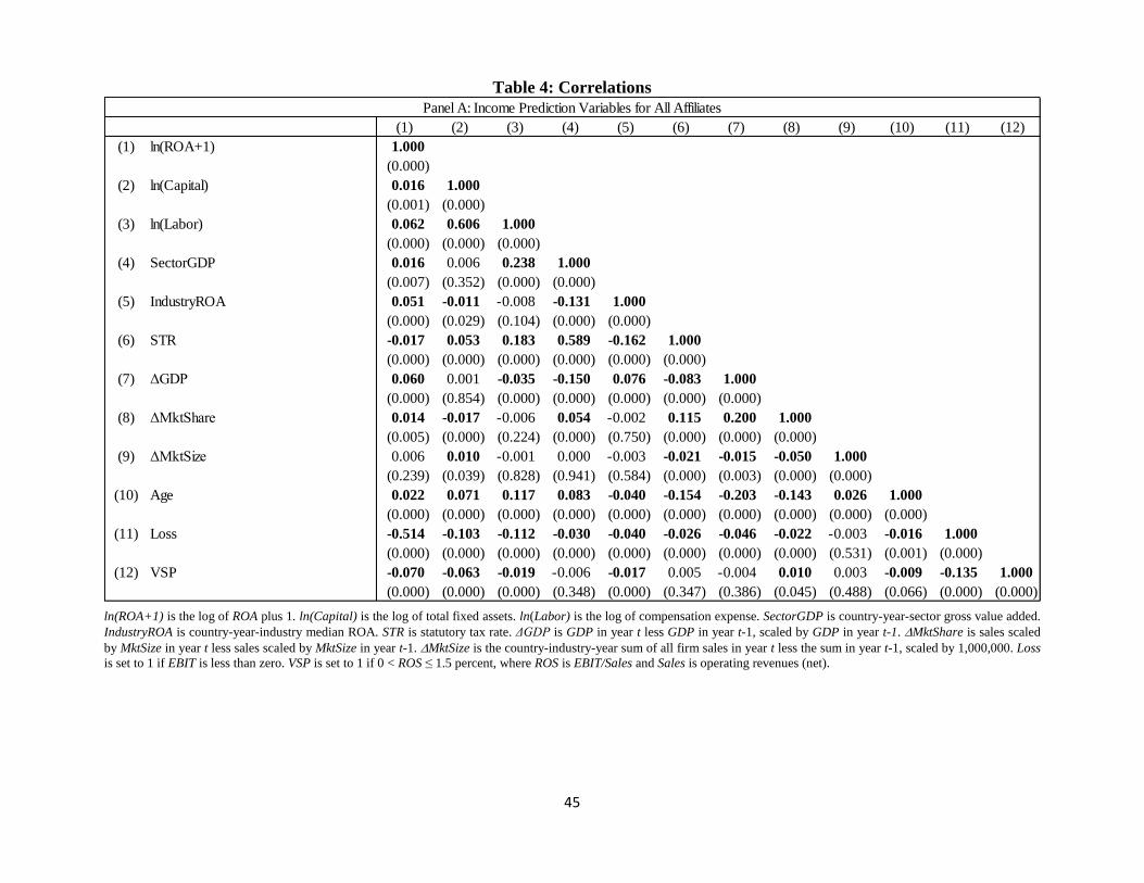
45
Table 4: Correlations
ln(ROA+1) is the log of ROA plus 1. ln(Capital) is the log of total fixed assets. ln(Labor) is the log of compensation expense. SectorGDP is country-year-sector gross value added.
IndustryROA is country-year-industry median ROA. STR is statutory tax rate. ΔGDP is GDP in year t less GDP in year t-1, scaled by GDP in year t-1. MktShare is sales scaled
by MktSize in year t less sales scaled by MktSize in year t-1. MktSize is the country-industry-year sum of all firm sales in year t less the sum in year t-1, scaled by 1,000,000. Loss
is set to 1 if EBIT is less than zero. VSP is set to 1 if 0 < ROS ≤ 1.5 percent, where ROS is EBIT/Sales and Sales is operating revenues (net).
(1) (2) (3) (4) (5) (6) (7) (8) (9) (10) (11) (12)
(1) ln(ROA+1) 1.000
(0.000)
(2) ln(Capital) 0.016 1.000
(0.001) (0.000)
(3) ln(Labor) 0.062 0.606 1.000
(0.000) (0.000) (0.000)
(4) SectorGDP 0.016 0.006 0.238 1.000
(0.007) (0.352) (0.000) (0.000)
(5) IndustryROA 0.051 -0.011 -0.008 -0.131 1.000
(0.000) (0.029) (0.104) (0.000) (0.000)
(6) STR -0.017 0.053 0.183 0.589 -0.162 1.000
(0.000) (0.000) (0.000) (0.000) (0.000) (0.000)
(7) ΔGDP 0.060 0.001 -0.035 -0.150 0.076 -0.083 1.000
(0.000) (0.854) (0.000) (0.000) (0.000) (0.000) (0.000)
(8) ΔMktShare 0.014 -0.017 -0.006 0.054 -0.002 0.115 0.200 1.000
(0.005) (0.000) (0.224) (0.000) (0.750) (0.000) (0.000) (0.000)
(9) ΔMktSize 0.006 0.010 -0.001 0.000 -0.003 -0.021 -0.015 -0.050 1.000
(0.239) (0.039) (0.828) (0.941) (0.584) (0.000) (0.003) (0.000) (0.000)
(10) Age 0.022 0.071 0.117 0.083 -0.040 -0.154 -0.203 -0.143 0.026 1.000
(0.000) (0.000) (0.000) (0.000) (0.000) (0.000) (0.000) (0.000) (0.000) (0.000)
(11) Loss -0.514 -0.103 -0.112 -0.030 -0.040 -0.026 -0.046 -0.022 -0.003 -0.016 1.000
(0.000) (0.000) (0.000) (0.000) (0.000) (0.000) (0.000) (0.000) (0.531) (0.001) (0.000)
(12) VSP -0.070 -0.063 -0.019 -0.006 -0.017 0.005 -0.004 0.010 0.003 -0.009 -0.135 1.000
(0.000) (0.000) (0.000) (0.348) (0.000) (0.347) (0.386) (0.045) (0.488) (0.066) (0.000) (0.000)
Panel A: Income Prediction Variables for All Affiliates

46
Table 4: Correlations (cont.)
Max_TP_RiskFt is a group-year measure of transfer pricing risk from 0 to 4, where 0 represents the least risk. STRit is statutory tax rate. CB/CF_Valueit equals zero when carryback
or carryforward is not allowed, carryback will not generate an immediate refund due to persistent losses, and the carryforward will not be used within two years. Loss_Scrutinyit is
an indicator variable equal to 1 if country-year transfer pricing risk is higher for reported affiliate losses.
Max_TP_RiskFt, STRit, CB/CF_Valueit, and Loss_Scrutinyit are as defined in Panel B. LSTRFt , CB/CF_ValueFt, and Loss_ScrutinyFt are the weighted average values for loss
affiliates in the same group-year, for STRit, CB/CF_Valueit, and Loss_Scrutinyit respectively, weighted by assets or labor. Rel_Activityit is alternatively profitable affiliate total
assets scaled by the sum of group-year total assets or total compensation expense scaled by the sum of group-year total compensation expense.

47
Table 5: Profit Prediction Model
ln(+1) = β0 + β1*ln(Capital) + β2*ln(Labor) + β3*Productivity + β4*TaxRate + β5*Shock + β6*VSP + β7*VSP*Shock + β8*Loss +
β9*Loss*Shock
This table estimates the profit prediction model on a sample of 41,199 European affiliate-years 2003-2012 with at least one foreign affiliated firm also located in Europe and
sufficient data from Amadeus and the European Commission for estimation. ln(ROA+1) is the natural log of EBIT scaled by TotalAssets plus 1. ln(Capital) is that natural log of
total fixed assets. ln(Labor) is the natural log of compensation expense. In column (1), Productivity is SectorGDP, a measure of country-year-sector gross value added as reported
by the European Commission. In column (2), Productivity is IndustryROA, a measure of country-year-industry median ROA. STR is the affiliate’s statutory tax rate. ΔGDP is GDP
in year t less GDP in year t-1, scaled by GDP in year t-1. MktShare is affiliate sales scaled by MktSize in year t less affiliate sales scaled by MktSize in year t-1. MktSize is the
country-industry-year sum of all affiliate and standalone firm sales in year t less the sum in year t-1, scaled by 1,000,000. Age equals year t minus the year the affiliate first appears
in the Amadeus database. VSP is set to 1 if 0 < ROS ≤ 1.5 percent, where ROS is EBIT/Sales and Sales is operating revenues (net). Loss is set to 1 if affiliate EBIT is less than zero.
All specifications include standard errors clustered by group. *, **, and *** represent two-tailed statistical significance at the 10%, 5%, and 1% levels, respectively.
Dependent Variable
Prediction X X*VSP X*Loss X X*VSP X*Loss
Intercept 0.1748 *** -0.1190 *** -0.3739 *** 0.1632 *** -0.1204 *** -0.3970 ***
(0.0141) (0.0050) (0.0281) (0.0117) (0.0044) (0.0244)
ln(Capital) - -0.0055 *** -0.0057 ***
(0.0009) (0.0008)
ln(Labor) + 0.0039 *** 0.0054 ***
(0.0012) (0.0009)
Productivity + 0.0111 *** 0.0126 ***
(0.0041) (0.0041)
STR - -0.1936 *** -0.0955 ***
(0.0390) (0.0226)
ΔGDP + 0.1021 *** -0.1076 *** 0.3490 *** 0.1179 *** -0.1268 *** 0.2583 **
(0.0194) (0.0231) (0.1159) (0.0184) (0.0211) (0.1038)
ΔMktShare + 0.0000 * -0.0000 -0.0000 0.0000 * -0.0000 0.0000
(0.0000) (0.0000) (0.0000) (0.0000) (0.0000) (0.0000)
ΔMktSize - -0.0009 0.0043 *** 0.0042 -0.0004 0.0030 *** 0.0054
(0.0007) (0.0011) (0.0068) (0.0005) (0.0009) (0.0054)
Age + -0.0098 *** 0.0045 * 0.0573 *** -0.0076 *** 0.0057 *** 0.0667 ***
(0.0028) (0.0027) (0.0139) (0.0021) (0.0021) (0.0111)
Sample
Productivity measure
N
adj. R-sq
Cluster
FE No
0.2936
All All
SectorGDP
Group
No
0.2881
Group
(2)
ln(ROA+1)
(1)
27,198 41,199
IndustryROA
ln(ROA+1)

48
Table 6: Determinants of Unexplained Profitability of Unprofitable Affiliates
Residit = β0 + 1*Max_TP_RiskFt + 2*STRit + 3*CB/CF_Valueit
+ 4*Loss_Scrutinyit + FE
This table tests the tax benefits and costs of achieving a shift-to-loss strategy on a sample of unprofitable affiliates.
The dependent variable is the residual from the income prediction model reported in Table 5 on the full sample of
41,199 European affiliate-years over the period 2003-2012 with at least one foreign affiliated firm also located in
Europe and sufficient data from Amadeus and the European Commission for estimation. Column (1) uses the
residual from estimating income using SectorGDP as the measure of Productivity, where SectorGDP is a measure
of country-year-sector gross value added as reported by the European Commission. Column (2) uses the residual
from estimating income using IndustryROA as the measure of Productivity, where IndustryROA is a measure of
country-year-industry median ROA. Max_TP_RiskFt is a group-year measure of EY’s country-year rating of
transfer pricing risk from 0 to 4, where 0 represents the least risk. STRit is statutory tax rate. CB/CF_Valueit equals
zero when carryback or carryforward is not allowed, when carryback will not generate an immediate refund due to
persistent losses, or when the carryforward will not be used within two years, assuming perfect foresight.
Loss_Scrutinyit is an indicator variable equal to 1 if country-year transfer pricing risk is higher for reported
affiliate losses. All specifications include industry, and year fixed effects and clustered standard errors by group. *,
**, and *** represent two-tailed statistical significance at the 10%, 5%, and 1% levels, respectively.
Productivity measure
Prediction
Intercept 40.5920 ** 18.5551 ***
(16.8087) (7.0850)
Max_TP_RiskFt - 0.0033 -0.0010
(0.0168) (0.0171)
STRit + 0.1846 0.2284 *
(0.1429) (0.1246)
CB/CF_Valueit - 0.0870 *** 0.0949 ***
(0.0204) (0.0128)
Loss_Scrutinyit + 0.0363 ** 0.0048
(0.0142) (0.0118)
Sample
N
adj. R-sq
Cluster
Industry / Year FE
Loss affiliates
Sector GDP Industry ROA
(1) (2)
Loss affiliates
4,361
0.0772
Group
Yes
Group
Yes
6,962
0.0577

49
Table 7: Determinants of Unexplained Profitability of Profitable Affiliates
Residit = β0 + 1*Max_TP_RiskFt + 2*LSTRFt + 3*CB/CF_ValueFt + 4*Loss_ScrutinyFt + 5*Rel_ActivityFt + FE
This table tests the tax benefits and costs of achieving a shift-to-loss strategy on a sample of profitable affiliates. The dependent variable is the
residual from the income prediction model reported in Table 5 on the full sample of 41,199 European affiliate-years over the period 2003-2012.
Column (1) uses the residual from estimating income using the Productivity measure SectorGDP, a measure of country-year-sector gross value
added as reported by the European Commission. Column (2) uses the residual from estimating income using Productivity measure IndustryROA,
a measure of country-year-industry median ROA. Max_TP_RiskFt is a group-year measure of EY’s country-year rating of transfer pricing risk
from 0 to 4, where 0 represents the least risk. LSTRFt is the weighted average STRit of loss affiliates in the same group-year, where STRit is
statutory tax rate. CB/CF_Valueit equals zero when carryback or carryforward is not allowed, when carryback will not generate an immediate
refund due to persistent losses, or when the carryforward will not be used within two years, assuming perfect foresight. CB/CF_ValueFt is the
weighted average CB/CF_Valueit of loss affiliates in the same group-year. Loss_Scrutinyit is an indicator variable equal to 1 if country-year
transfer pricing risk is higher for reported affiliate losses. Loss_ScrutinyFt is the weighted average Loss_Scrutinyit for loss affiliates in the same
group-year. Rel_Activityit is either profitable affiliate total assets scaled by the sum of group-year total assets or profitable affiliate total
compensation expense scaled by the sum of group-year total compensation expense. All specifications include industry, and year fixed effects
and clustered standard errors by group. *, **, and *** represent two-tailed statistical significance at the 10%, 5%, and 1% levels, respectively.
Recommended