University of Amsterdam
MSc PhysicsTheoretical Physics
Master Thesis
Quantum Monte Carlo simulations for the Bose-Hubbard modelExploring new parameter regimes for quantum simulation
by
Etienne van Walsem
6148204
September 2015
60 ECTS
Research carried out between September 2014 and October 2015
Supervisor:Dr. Philippe Corboz
Examiner:Dr. Robert Spreeuw
Institute for Theoretical Physics

Abstract
In this thesis we simulate the Bose-Hubbard model with quantum Monte Carlo techniques. We use thedirected worm algorithm. We investigate the normal fluid to superfluid phase transition of the Bose-Hubbard model in the Kagome lattice. The phase diagram is found to have a similar shape as the phasediagram of the square lattice, but with lower temperatures. We investigate parameter regions relevantfor experiments done in the quantum gases and quantum information group of the UvA. We show thatthere are Mott-insulating, normal fluid and superfluid phases in the parameter regime between t
U = 0.14and t
U = 0.02. We mimic disorder for the same systems and find that for disorder of ∆ = 0.05U and∆ = 0.1U there is little effect on the density and superfluid stiffness of the system, but for a disorder of∆ = 0.2U there is a clear difference. Kagome superlattices on top of triangular lattices are investigatedas well. It is found that Kagome superlattices created by lowering the chemical potential at certainlattice sites gives the same physics as the intended Kagome lattice. For a change in the local chemicalpotential of δ = 20U the Kagome superlattice is clearly visible, for δ = 0.2U the superlattice is notvisible at all, and for δ = 0.5U the Kagome superlattice is only visible for µ < 0.4. The influences offences on periodic systems are compared to open systems. Here we see that fences with a height in therange of 2U − 10.5U give similar results.

Acknowledgements
First of all I would like to thank my supervisor Philippe Corboz guiding me through this project andteaching me about computation techniques as well as physics. Furthermore I would like to thank Arthurla Rooij for coming up with the project, helping me to understand the experiment and helping with thecomputations of the experimental parameter region. It was a pleasant cooperation. Thanks to Tama Mafor taking his time and helping to understand the DWA source code. And finally, thanks to Sarah andKoen for proofreading this thesis for grammar and spelling.

Nederlandse samenvatting
In deze thesis is het Bose-Hubbard model gesimuleerd met behulp van kwantum Monte Carlo techniek.Dit is gedaan om toekomstige experimenten een idee te geven over wat voor soort natuurkundige systemze kunnen verwachten.
Het Bose-Hubbard model is een model dat beschrijft hoe kwantumdeeltjes op een rooster bewegen.Het model heeft drie parameters. De eerste parameter is de hop-parameter die beschrijft hoe makkelijkdeeltjes naar aanliggende roosterpunten kunnen verplaatsen. De tweede parameter is de plaatselijkeinteractieparameter die aangeeft in wat voor mate de deeltjes elkaar afstoten. De laatste parameter is eenchemische potentiaal: deze reguleert hoeveel deeltjes in het totale systeem zitten. De kwantumdeeltjeszijn in ons geval zogenaamde bosonen, wat inhoudt dat er meerdere van de zelfde soort deeltjes op eenplaats kunnen zijn. Er bestaan ook andere deeltjes, fermionen, die niet op dezelfde plek kunnen zitten.Afhankelijk van de verhoudingen tussen deze parameters zijn de deeltjes in verschillende fases. De Mott-isolerende-fase, de vloeistof-fase en de superfluıde-fase. De Mott-isolerende-fase komt voor als er precieseen geheel aantal deeltjes per roosterpunt is en de invloed van de plaatselijke interactie groter is dan dievan het verplaatsen. Dit betekent dat er geen deeltjes meer door het systeem bewegen omdat ze op elkroosterpunt afgestoten worden.
Als de hop-parameter veel groter is dan de plaatselijke interactie kunnen de deeltjes door het systeembewegen. Als de temperatuur van het systeem zich op het absolute nulpunt bevindt zijn de deeltjesin de superfluıde-fase, wat inhoudt dat de deeltjes geen viscositeit meer hebben en wrijvingsloos doorhet systeem bewegen. Op temperaturen boven het nulpunt ontstaat er de vloeistof-fase tussen de Mott-isolerende-fase en de superfluıde-fase.
Dit lijkt allemaal overzichtelijk, maar is het niet. Het is nog niet bekend hoe we de beweging vande deeltjes kunnen beschrijven in een twee-dimensionaal rooster. Ook is het niet bekend in welke fasehet systeem is bij bepaalde temperaturen en parameterverhoudingen. Gelukkig is dit wel te simulerenmet computers. Het doel van deze thesis is om met computersimulaties te laten zien wat experimentelegroepen kunnen verwachten met bosonische deeltjes.
Het experiment waar we dit voor doen is bezig met kwantumsimulatie. Daar bootsen ze een systeemna, zoals het Bose-Hubbard model, op een manier waar ze de parameters van het systeem kunnen contro-leren en de observabelen kunnen meten. Dit is een toevoeging op de berekeningen en computersimulatiesomdat computersimulaties niet mogelijk zijn voor fermionsiche deeltjes.
Voor onze computersimulaties hebben we kwantum Monte Carlo technieken gebruikt. Monte Carlotechniek maakt gebruik van willekeurige getallen om steekproeven van natuurkundige systemen te si-muleren. Vanuit die steekproeven kan een gemiddelde bepaald worden. Bijvoorbeeld kunnen we in onsBose-Hubbard model steekproeven van de dichtheid en superfluıditeit nemen. Het voordeel van eenMonte Carlo simulatie is dat hoe meer steekproeven je neemt hoe nauwkeuriger je antwoord wordt.
Omdat het systeem wat onderzocht word kwantummechanisch is gebruiken we kwantum Monte Carlotechnieken. Hierin beschrijven we het 2-dimensionale systeem in een 2+1-dimensionele wereldlijnenrepresentatie. Vervolgens maken we steekproeven met behulp van het directed worm algoritme.
In deze thesis hebben we deze techniek toegepast op wat er in de experimenten gedaan gaat worden.Zo hebben we gekeken naar welke fase het systeem zich in bevind binnen de regio waar het systeemexperimenteel gesimuleerd gaat worden. Ook of de methodes werken om verschillende roosterconfiguratieste maken en deeltjes in het systeem te vangen. En of er effect op de fysica van het systeem is van de
wanorde tussen de verschillende roosterpunten wat fundamenteel in het experiment voorkomt . Alslaatste hebben we gekeken bij welke temperaturen de overgang van de superfluıde fase naar de normalevloeistof fase gebeurd. Dit was al bekend voor het vierkante rooster en dit hebben wij nu ook gesimuleerdvoor het Kagome rooster.
In deze thesis is er gevonden dat het systeem alle drie de fases (Mott-isolerend, normale vloeistofen superfluıde) voorkomen in het regime waarin het experiment word uitgevoerd. De methodes omverschillende roosterconfiguraties te maken en om de deeltjes in het systeem te vangen werken, mits dejuiste parameters worden gebruikt. Wanorde op kleine schaal heeft nauwelijks invloed op de fysica. Ende overgangs temperatuur voor de superfluıde naar normale vloeistof fase is lager in het Kagome roosterdan in het vierkante rooster.
Contents
1 Introduction 1
2 Theory 22.1 Ultra-cold atoms in lattices and the Bose Hubbard model . . . . . . . . . . . . . . . . . . 2
2.1.1 Cold atom lattice physics . . . . . . . . . . . . . . . . . . . . . . . . . . . . . . . . 22.1.2 Wannier states . . . . . . . . . . . . . . . . . . . . . . . . . . . . . . . . . . . . . . 3
2.2 Phase diagram of the Bose-Hubbard model . . . . . . . . . . . . . . . . . . . . . . . . . . 32.2.1 Superfluid phase U
t � 1 . . . . . . . . . . . . . . . . . . . . . . . . . . . . . . . . . 42.2.2 Mott-insulating phase t
U � 1 . . . . . . . . . . . . . . . . . . . . . . . . . . . . . . 42.2.3 Phase transition . . . . . . . . . . . . . . . . . . . . . . . . . . . . . . . . . . . . . 5
2.3 Superfluid to normal fluid phase transition . . . . . . . . . . . . . . . . . . . . . . . . . . . 52.3.1 Berezinskii-Kosterlitz-Thouless transition . . . . . . . . . . . . . . . . . . . . . . . 6
3 Numerical methods 83.1 The Monte Carlo method . . . . . . . . . . . . . . . . . . . . . . . . . . . . . . . . . . . . 8
3.1.1 Markov Chains . . . . . . . . . . . . . . . . . . . . . . . . . . . . . . . . . . . . . . 83.1.2 Errors and correlations . . . . . . . . . . . . . . . . . . . . . . . . . . . . . . . . . . 9
3.2 The Ising model . . . . . . . . . . . . . . . . . . . . . . . . . . . . . . . . . . . . . . . . . 93.2.1 Clusters and the Wolff algorithm . . . . . . . . . . . . . . . . . . . . . . . . . . . . 103.2.2 Simulating the Ising model . . . . . . . . . . . . . . . . . . . . . . . . . . . . . . . 11
3.3 Worldline representation . . . . . . . . . . . . . . . . . . . . . . . . . . . . . . . . . . . . . 113.3.1 The Worm algorithm . . . . . . . . . . . . . . . . . . . . . . . . . . . . . . . . . . . 123.3.2 Observables . . . . . . . . . . . . . . . . . . . . . . . . . . . . . . . . . . . . . . . . 14
4 Normal fluid to superfluid phase transition 164.1 Normal to superfluid . . . . . . . . . . . . . . . . . . . . . . . . . . . . . . . . . . . . . . . 164.2 Method . . . . . . . . . . . . . . . . . . . . . . . . . . . . . . . . . . . . . . . . . . . . . . 164.3 Simulations . . . . . . . . . . . . . . . . . . . . . . . . . . . . . . . . . . . . . . . . . . . . 17
4.3.1 Literature comparison . . . . . . . . . . . . . . . . . . . . . . . . . . . . . . . . . . 174.3.2 Kagome lattice . . . . . . . . . . . . . . . . . . . . . . . . . . . . . . . . . . . . . . 17
5 Mott-superfluid phase transition 215.1 Method . . . . . . . . . . . . . . . . . . . . . . . . . . . . . . . . . . . . . . . . . . . . . . 215.2 Result . . . . . . . . . . . . . . . . . . . . . . . . . . . . . . . . . . . . . . . . . . . . . . . 22
5.2.1 Literature comparison and finite temperature and finite size effects . . . . . . . . . 225.2.2 Results of the experimental region . . . . . . . . . . . . . . . . . . . . . . . . . . . 22
6 Superlattices 276.1 Introduction . . . . . . . . . . . . . . . . . . . . . . . . . . . . . . . . . . . . . . . . . . . . 276.2 Results . . . . . . . . . . . . . . . . . . . . . . . . . . . . . . . . . . . . . . . . . . . . . . . 27
6.2.1 Smaller δ . . . . . . . . . . . . . . . . . . . . . . . . . . . . . . . . . . . . . . . . . 28
i
CONTENTS
7 Disorder and trapping atoms in magnetic lattices 317.1 Disorder . . . . . . . . . . . . . . . . . . . . . . . . . . . . . . . . . . . . . . . . . . . . . . 31
7.1.1 Simulating disorder . . . . . . . . . . . . . . . . . . . . . . . . . . . . . . . . . . . . 317.2 Trapping atoms in finite magnetic lattices . . . . . . . . . . . . . . . . . . . . . . . . . . . 32
8 Conclusion and outlook 358.1 Conclusion . . . . . . . . . . . . . . . . . . . . . . . . . . . . . . . . . . . . . . . . . . . . 358.2 Outlook . . . . . . . . . . . . . . . . . . . . . . . . . . . . . . . . . . . . . . . . . . . . . . 36
ii
Chapter 1
Introduction
’Nature isn’t classical, dammit, and if you want to make a simulation of nature, you’d better make itquantum mechanical, and by golly it’s a wonderful problem, because it doesn’t look so easy.’
- R.P. Feynman
Understanding highly correlated quantum systems is a big challenge in modern physics. Analyticaland numerical methods have not been capable of solving the current problems. To get a better under-standing of those systems Richard Feynman proposed in 1982 that a quantum simulator can be used toinvestigate quantum systems. Here a quantum simulator is where a controlled quantum system is usedto investigate the behaviour and proporties of an uncontrollable quantum system [1].
In this thesis the Bose-Hubbard model has been investigated. There is no full analytical solutionknown for this model. Numerical methods such as Quantum Monte Carlo methods are capable to givenew insights in this model. For the fermionic version of the Hubbard model there is no analytical solutionknown either. And due to the infamous negative sign problem Monte Carlo simulations are not suitableto investigate this case as well. Quantum simulation would be a good method to further investigate the(Bose) Hubbard model.
One of the potential techniques to build a quantum simulator for the Hubbard model is ultra coldatoms in lattice traps. Jaksch et al. proposed it is possible to do such simulations with rubidium atomsin a BEC state in optical traps [2]. In 2001 Greiner et al. actually preformed the experiment [3]. Inthat experiment known states of the Bose-Hubbard model are found such as the Mott insulating phaseand superfluid phase. This technique is limited by the atom laser interactions, in nearly all latticesthe minimal lattice spacing is 450 nanometer. Other parameter regimes of the Hubbard model can beinvestigated if the lattice spacing decreases. Currently there is a lot of scientific activity in developingnew techniques for trapping ultra cold atoms which can lead to smaller lattice spacings so that newparameter regimes can be studied.
New techniques include ultra cold atoms trapped in magnetic lattices [4, 5], atoms trapped in evan-escent fields [6] and photonic crystals [7].
Another perk of the magnetic trap is that the trapping potential is a box potential instead of anharmonic potential in the optical case. This leads to a better understanding of the particle density inthe superfluid phase and also the possibility to research edge effects.
In this thesis benchmark simulations for this new parameter regimes will be presented. Togetherwith the Quantum Gases & Quantum Information group at the UvA we looked at which parameterregimes are feasible [8], and what the expected edge effects are from the trapping potential for differentparameter regimes. Simulations of the effects of a disordered local chemical potential to mimic disorderin experimental set ups are done as well. This is interesting for the new magnetic trap techniquesbecause, in an optical trap, there is some disorder between the different lattice sites. This thesis canplay an advisory role in what parameter regimes are interesting to study experimentally. In addition webenchmarked the critical temperature for the normal fluid to superfluid phase transition in the squareand Kagome geometry.
1
Chapter 2
Theory
2.1 Ultra-cold atoms in lattices and the Bose Hubbard model
2.1.1 Cold atom lattice physics
For describing ultra-cold Bosonic atoms in an external trapping potential we can write the Hamiltonianas:
H =
∫d3rψ†(r)
[− ~2
2m∇2 + VT(r) + V0(r)
]ψ(r) +
1
2gint
∫d3rψ†(r)ψ†(r)ψ(r)ψ(r) (2.1)
where m is the atom mass, VT the external trapping potential, V0 the lattice potential and gint thecoupling strength [9]. In the two dimensional case a possible lattice potential can be written as V0(x) =∑2j=1 Vj0 sin2(kxj) with k = 2π
λ , where λ is the periodicity of the lattice. In modern experiments theperiodicity lies in the range of 100 nm to 450 nm.
The atoms will be periodically localised by the potential V0. The standard approach to find the bandstructure is by only considering the kinetic and periodic potential terms of the Hamiltonian:
H = − ~2
2m
∂2
∂x2+
2∑j=1
Vj0 sin2(kxj). (2.2)
Due to periodic boundaries the momenta are quantised:
q =2πlλ2N
, l = 0, 1, . . . , N − 1. (2.3)
In order to rewrite equation (2.2) in dimensionless variables the following coordinate change is performed:
πz = kx
such that equation (2.2) becomes the eigenequation equation (2.4).− ∂2
∂z2+
2∑j=1
V ′j sin2(πzj)
ψ(z) = Eψ(z), (2.4)
where V ′ = π22m~2k2 V0 = π2
ERV0. This introduces the recoil energy ER which is used as an energy scale
for the lattice. The eigenstates ψ of equation (2.4) can be expected to have the form of Bloch wavefunctions: ψ(z) = eiqzunq(z). Here unq(z) is a function with the same periodicity as equation (2.4), qis the quantised momentum and n is the band index. In this case it is sufficient to do computations
2
CHAPTER 2. THEORY
with the lowest band only, n = 1. Combining all this, we finally obtain the following solvable differentialequation:
−(∂2
∂z2+ iq
)2
uq(z) +
2∑j=1
V ′j sin2(πzj)uq(zj) = Equq(z). (2.5)
2.1.2 Wannier states
In the atomic limit for lattices, where the lattice spacing is larger than the Bohr radius, the weight ofthe electron functions is tightly bound to the lattice centers. A Wannier basis is defined as:
|ψkn〉 =1√N
∑R
eik·R|ψRn〉 (2.6)
and the Wannier function ψRn(r) ≡ 〈r|ψRn〉. Where Rn denote the coordinates of the lattice sites.Wannier states are not eigenfunctions of the Hamiltonian but linear combinations of Bloch functions[10].
Wannier states localised around lattice sites Rn for N Bloch states uq(x) can be written as follows:
w(x−Rn) =1√N
∑q
eiq(x−Rn)uq(x). (2.7)
The Wannier function is often approximated by a Gaussian function:
w(x−Rn) =
(1
πaax
)1/4
e− (x−Rn)2
2a2ax , (2.8)
where aax =√
~mωax
, and ωax the harmonic oscillator length in the axial direction. [9]
The field operators in the lowest Wannier state can be be expanded as:
ψ(x) =∑i
biw(x−Ri), (2.9)
where bi is the boson annihilation operator. If we insert this in equation (2.1) we get the Bose-HubbardHamiltonian:
H = −t∑〈i,j〉
b†i bj +U
2
∑i
ni(ni − 1)− µ∑i
ni. (2.10)
having the following amplitudes:
ti,j = −∫dxw∗(x− xi)
(− d2
dx2+ V0 sin2(kx)
)w(x− xj)
U = gint
∫dxw4(x)
εi =
∫d3xVT (x)|w(x− xi)|2
(2.11)
For an homogeneous lattice we can write our chemical potential to µi = µ− εi or just µ [9, 2].
2.2 Phase diagram of the Bose-Hubbard model
At T = 0 two different phases are observed in the Bose-Hubbard model. When Ut � 1 the system is in
the superfluid phase and when tU � 1 in the Mott-insulating phase. In this section both phases will be
described briefly.
3
CHAPTER 2. THEORY
2.2.1 Superfluid phase Ut� 1
The dominant phase in the low T range is the superfluid phase. In a superfluid the particles behave asa fluid without viscosity. Superfluidity has been described by a two liquid fluid model, where superfluidand normal fluid particles are combined in the superfluid phase. The superfluid part of the liquid isassumed to carry zero entropy and to flow irrotationally, while the normal fluid part behaves as a fluidwe are used to, for example H2O. In the superfluid phase the fraction of superfluid particles is non zero;thus not necessarily one. This model was proposed by Laszlo Tisza in 1938 [11].
The microscopic description of a superfluid can be written from the generalised condensate wavefunction χ(~x) = eiθ(~x)|χ(~x)|. The spatial variation of phase θ(~x) is used to describe a velocity field vs:
~vs =~m~∇θ(~x), (2.12)
with m the mass per particle.This velocity is irrotational by definition (∇× vs = 0) and one can observethere is no ‘ignorance’ in the state χ thus the entropy must be carried entirely by the normal component.The two assumptions of the two fluid model are thus fulfilled [11, 12].
An expression for the superfluid fraction can be derived in the macroscopic framework. For simplicitywe derive this equation in the one dimensional case. Here we assume an imposed linear phase variationθ(x) with a total phase difference of Θ over the system length L. So θ(x) = Θx/L. This creates a flowwith velocity
vs =~Θ
mL.
The part of the system which responds to the phase difference and thus flows with this velocity issuperfluid. The increase in energy between the original state’s ground state energy E0 and the groundstate energy of the system with the phase variation EΘ can be accounted to the kinetic energy of thesuperfluid flow
EΘ − E0 =1
2Msv
2s .
Here vs is the aforementioned velocity of the flow and Ms is the total mass of the superfluid portion.Assuming ms = fsmN we end with an expression for the superfluid fraction fs:
fs =2mL2
~NEΘ − E0
Θ=
I2
tN
EΘ − E0
Θfor θ � π. (2.13)
Here N is the total number of particles. It has to be noted that the twist Θ must be small for thisexpression to hold. In the last part of equation (2.13) we expressed the fraction for a lattice with thenumber of sites I, instead of the continuous case, and replace the kinetic prefactor ~2/(2m) with thetunnelling t [12].
2.2.2 Mott-insulating phase tU� 1
When tU � 1 the superfluid phase gets suppressed by the Mott-insulating phase. We follow the seminal
paper of Fisher et al. in the explanation below [13]. To describe this phase let us first consider the caset = 0. Here all the lattice sites are completely decoupled from each other. This means that each site isoccupied by a positive integer number of bosons. Our Hamiltonian now gives the following expressionfor the onsite energy:
ε(n) = −µn+1
2Un(n− 1) (2.14)
4
CHAPTER 2. THEORY
This shows that there is an occupation of an integer number, n, of bosons per site dependent on thefraction µ/U . The relation can be shown as:
〈n(µ/U)〉 =
0 µ/U < 0
1 0 < µ/U < 1
2 1 < µ/U < 2...
n n− 1 < µ/U < n
Now we proceed with the t 6= 0 case. Imagine a fixed µU = n− 1
2 +α with − 12 < α < 1
2 so that the densityis still fixed on n. The energy required to add or remove a particle is δEp ∼ ( 1
2 −α)U or δEh ∼ ( 12 +α)U .
Ep to denote the energy to add an particle and Eh an hole respectively. Suppose the hopping t is smallerthen δEp and δEh; this means that the kinetic energy gained to move a particle is smaller than the lostenergy to overcome the lost potential by adding or removing a particle. So there exists a finite region inthe µ− t plane where the density of particles n is constant. Moreover, in that region the energy gain tis smaller than the cost in potential energy δEp + δEh, therefore hops are energetically costly. It follows
that the probability of a boson hopping r number of sites is proportional to(
tδEp+δEh
)or exp(−r/ξ)
where ξ ∼ [ln((δEp + δEh)/J)]−1. Thus in the region of constant integer n the density fluctuations
are localised in a volume of linear size ξ. And lastly the region is incompressible because ∂ρ∂µ vanishes
everywhere in that region. The states are Mott states [13].
The shape of the Mott-insulating region in the µ− t plane can be obtained from the mean field valueof the ground state by applying the usual Landau argument for second order phase transitions throughexpanding this energy in powers of ψB:
E0 = E00 + r|ψB|2 +O(|ψB|4).
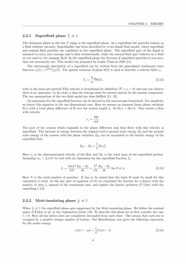
The boundary of the Mott-insulating region is now where r changes sign [14]. See figure 2.1 for the phasediagram and the shape of the Mott-insulating region.
2.2.3 Phase transition
The phase transition between this superfluid phase and Mott-insulating phase is at a certain quantumcritical point (QCP) which is in the 2D case at U
t = 29.34(2) [15]. In the extreme cases Ut � 1 and
tU � 1 the two phases can be described using perturbation theory. One of the motivations to study theBose-Hubbard model numerical is to better understand the transition between these two phases [9].
2.3 Superfluid to normal fluid phase transition
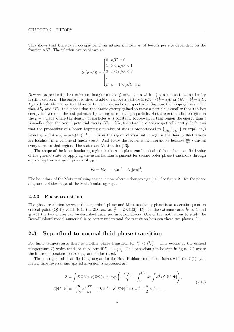
For finite temperatures there is another phase transition for Ut <
(Ut
)c. This occurs at the critical
temperature Tc which tends to go to zero if Ut →
(Ut
)c. This behaviour can be seen in figure 2.2 where
the finite temperature phase diagram is illustrated.
The most general mean-field Lagrangian for the Bose-Hubbard model consistent with the U(1) sym-metry, time reversal and spatial inversion is expressed as:
Z =
∫DΨ∗(x, τ)DΨ(x, τ) exp
(−V F0
T−∫ 1/T
o
dτ
∫ddxL[Ψ∗,Ψ]
),
L[Ψ∗,Ψ] = − ∂r∂µ
Ψ∗∂Ψ
∂τ+ |∂τΨ|2 + c2|∇Ψ|2 + r|Ψ|2 +
u
2|Ψ|4 + . . .
(2.15)
5
CHAPTER 2. THEORY
Figure 2.1: Zero temperature phase diagram for interacting bosons. The Mott-insulating phase is denotedby MI for small t/U and the superfluid phase is denoted by SF. Figure taken from Fisher et al. [13]
Here V is the total volume of the lattice and F0 is the free energy density of a system with decoupledsites [14]. The density of the Mott-insulating phase 〈n〉 is related to this free energy density as:
−∂F0
∂µ= 〈n〉.
In the r � 0 case the insulating phase is found and in the r � 0 the superfluid phase is found. Ifthe first term of equation (2.15), ∂r
∂µ , is zero the tangent at the tips in the Mott lobes is vertical, see
figure 2.1. When this term is zero equation (2.15) is the same as for the N = 2 quantum rotor modelor the (d+1)-dimensional XY model. This means that the phase transition between the Mott-insulatingand the superfluid phase is in the same universality class as the O(2) quantum rotor model [14]. It isshown that this transition is of the Berezinskii-Kosterlitz-Thouless (BKT) type [9, 16, 17].
2.3.1 Berezinskii-Kosterlitz-Thouless transition
The Berezinskii-Kosterlitz-Thouless transition was originally developed for the two-dimensional neutralsuperfluid and the XY model [17, 16]. The XY model is a two-dimensional spin model possessing a U(1)symmetry. This model is not expected to have a second order phase transition. This is a result of theordered phase being destroyed by transverse fluctuations, due to the broken continuous symmetry. WhatBerezinskii, and Kosterlitz and Thouless showed is that there is a phase transition due to topologicallong range order.
At low temperatures the vortex anti-vortex pair is likely to be close to another because of the Boltzmanfactor. On the other hand, in the high temperature case the Boltzman distribution is the other wayaround and we have a plasma of vortices. The transition between these situations is the BKT-phasetransition.
We can obtain the critical temperature as discussed by Kosterlitz and Thouless [16]. At large distancesfrom a vortex the strain produced is inversely proportional to the distance and so the energy of a single
6
CHAPTER 2. THEORY
Figure 2.2: Simplified scheme of the finite T phase diagram for interacting bosons in a lattice potentialat a filling of n = 1. Figure taken from Trotzky et al. [15]
vortex depends logarithmically on the size of the system. They show that the energy is given by:
E =vb2(1 + τ)
4πln
A
A0.
where v is the two-dimensional rigidity modulus, τ is the Poissons ratio, and A0 is an area of the orderof the Burgers vector squared, b2. The entropy associated with a vortex also depends logarithmically onthe area and is shown to be:
S = kB lnA
A0+O(1).
where kB is the Boltzmann constant. Since both energy and entropy depend on the size of the system inthe same way, the energy term will dominate the free energy at low temperatures, and the probability ofa single dislocation appearing in a large system will be negligible small. At high temperatures, vorticeswill appear spontaneously when the entropy term takes over. For a superfluid this will be:
kBTc =π~2ρs
2m(2.16)
where ρs is the superfluid density. This is also referred to as the Nelson-Kosterlitz jump [18]. Thiscritical temperature is also the temperature where the free energy changes sign.
7
Chapter 3
Numerical methods
3.1 The Monte Carlo method
The Monte Carlo method is a computational method which is widely used within physics. In thisthesis the Monte Carlo method is used as well. The method is advantageous for doing high-dimensionalintegrals and evaluation of exponentially large sums.The efficiency of the method is, unlike in othermethods, independent on the number of dimensions of the integral. Monte Carlo makes use of randomsampling to obtain statistical results. Monte Carlo was invented in 1946 by Stanislaw Ulam. Theinspiration of the method came from determining the winning percentage of a game of Solitaire. Insteadof using combinatory calculus the estimation is done by playing a finite number of Solitaire games witha random shuffled card desks. One can estimate the total winning percentage by taking the winningpercentage of the finite number of games. The precision of the answer can be improved by increasing thesize of your limited set. Ulam, in cooperation with von Neumann, used this method in the Manhattanproject to estimate neutron multiplication rates in order to predict explosive behaviour of fission weapons[19]. The method is considered useful for multiple fields of physics, including condensed matter physics,the topic of this thesis.
3.1.1 Markov Chains
A Markov chain is a random process on a chain of states. The process forms pseudo random numbersaccording to a arbitrary probability p. Every state, x, in the Markov chain can transform into anotherstate, y, with a certain probability. Those probabilities can be represented in a transition matrix Wxy
for which holds that the total probability to transform from any state x to a certain state y is one. TheMarkov Chain and transformation matrix have to fulfil ergodicity and detailed balance to sample thedesired distribution given by p.
Ergodicity holds if it is possible to reach any state y from state x in a finite number of steps. In otherwords, for every x and y, ∃n0 <∞|∀n > n0 : (Wn)xy 6= 0.
Detailed balance holds if
Wxy
Wyx=pypx. (3.1)
Here px and py are distributions in equilibrium. At each step the probability p(n)x changes, it will converge
to this equilibrium distribution px for which the detailed balance condition equation (3.1) holds.A Monte Carlo method based on Markov Chains is the Metropolis Algorithm, introduced by Metro-
polis in 1953 [20]. The algorithm starts with a random point xi. At the next step we propose a randomnew point x′ = xi + ∆x and accept that point with a probability P = px′
pxi. By accepting we mean:
xi+1 = x′, and by not accepting xi+1 = xi. If P ≥ 1 the new point is accepted by default. If P < 1 wedraw a random number r in the interval [0,1[ and accept the new point if r < P holds, and reject it if
8
CHAPTER 3. NUMERICAL METHODS
does not hold. Theses steps are repeated for random new points to gain a set of samples. Measurementscan be performed on the set of samples.
This algorithm is ergodic if all the finite possible random changes, x′ = xi + ∆x, allow all points inthe domain to be reached in a finite number of steps. And for each change ∆x there should be a change−∆x such that detailed balance holds:
Wij
Wji=
1Nmin(1, p(j)/p(i))1Nmin(1, p(i)/p(j))
=p(j)
p(i).
Here N is the number of possible random changes.
3.1.2 Errors and correlations
In Monte Carlo simulations the error of an observable O for N number of uncorrelated samples scalesas:
∆O =
√Var O
N. (3.2)
Here we have to take into account the possible correlation between successive points xi. The correlationof two observables Oi and Oi+δ decays exponentially as follows:
〈OiOi+δ〉 − 〈O〉2 ∝ exp−δτO
. (3.3)
Here we can see that the error on the observable ∆O diverges to its true value for δ → ∞, with anautocorrelation time τO. To obtain a reliable statistical error a binning analysis can be performed. Herea new ’binned’ series is created iteratively by equation (3.4), were subsequently the average and error ofthis new binned series can be determined.
O(l)i =
1
2(O
(l−1)2i−1 +O
(l−1)2i ) (3.4)
The errors on the averages of O(l) are less correlated than for the previous averages, the new error willbe larger than the previous error. By iteratively creating new binned series the error will converge to itstrue value. The mean value stays the same.
3.2 The Ising model
The metropolis algorithm has proven to be successful in solving the classical Ising model. The Isingmodel describes a spin system with nearest neighbouring spin interaction, a spin can either point up(+1) or down (-1). The hamiltonian is written as:
H = −J∑〈i,j〉
σiσj . (3.5)
Here the J gives the strength of the coupling of two neighbouring spins σi and σj . The Ising model isviewed as a simple model for magnetism where in the case J > 0 it describes a ferromagnet and in thecase J < 0 an anti-ferromagnet.
The Metropolis algorithm for the Ising model works as follows:
1. Start with an random spin configuration x0
2. Propose a spin-flip on a random lattice site resulting in a new configuration xnew. Accept thisspin-flip with probability P = e−β∆E . Here β is the inverse temperature and ∆E is the energydifference of the spin configuration for the proposed spin-flip. P is determined as the fraction ofthe two probabilities of the two configurations with energy Ei: pi = e−βEi/Z.
9
CHAPTER 3. NUMERICAL METHODS
3. If the flip is accepted continue with a new configuration xn+1 = xnew
4. If the flip is rejected continue with the previous configuration xn+1 = xn
5. Repeat the aforementioned step N times. Before taking measurements run a finite number of spin-flips to ’thermalise’ the spin configuration. It is conventional to do measurements each sweep wherea sweep is a series of Ns single spin flips, where Ns is the number of spins in the system.
This is ensured to be ergodic since every possible spin configuration can be reached in a finite numberof steps.
3.2.1 Clusters and the Wolff algorithm
The single flip metropolis algorithm is shown to be inefficient around the critical temperature. Theautocorrelation time (τ), the typical time scale for two measurements to be uncorrelated, is shown todiverge as τ ≈ [min(L, ξ)]z, where at Tc, ξ →∞. For the single flip algorithm the critical exponent z isfound to be 2. To improve the precision around the critical temperature, cluster based algorithms aredeveloped, such as the Wolff algorithm [21].
All cluster algorithms are built on the Kandel-Domany framework which is a generalised version ofthe Fortuin-Kastelyn representation of the Ising model [22, 23]. In this framework the partition functionis written as a set of possible graphs G of each configuration C in the set of all possible configurations C.
Z =∑C∈C
∑G∈G
W (C,G),∑G∈G
W (C,G) = W (C) := e−βEC
(3.6)
Here we used Ec as the energy of the configuration C. In the method a graph G ∈ G is assigned tothe configuration C with the probability PC(G) = W (C,G)/W (C). Subsequently a new configurationis chosen with probability p[(C,G) → p(C ′, G)]. Here the graph G is kept fixed and the probability,p, can be determined by e.g. the Metropolis algorithm. Next a new graph can be chosen for the newconfiguration. The method simplifies if a graph mapping is found for which the weights are independent ofthe configuration, providing the weights are non-zero. Therefore we want the weights to be W (C,G) =∆(C,G)V (G) with ∆ = 1 for non-zero weights and ∆ = 0 for a weight of zero. This means in theMetropolis algorithm that p = 1 [24].
The Wolff algorithm is where this method is used for the Ising model. The graphs are bond graphs, abond can be between two neighbouring sites. Two spins pointing in the same direction can be connectedor disconnected. Two spins pointing in opposite directions are disconnected by default. For the Isingmodel the weights are:
W (C) =∏b
w(Cb),
W (C,G) =∏b
w(Cb, Gb) =∏b
∆(Cb, Gb)V (Gb).(3.7)
The Wolf algorithm goes as follows:
1. Pick a random spin.
2. Add neighbouring spins to the cluster pointed in the same direction with probability p = 1 −exp(−2βJ).
3. Repeat the previous step until no spins are added to the cluster.
4. Flip all spins in the cluster.
There are improved estimators for this algorithm which speed up the process [24, 21]. An alternativecluster algorithm is the Swendsen-Wang algorithm [25].
10
CHAPTER 3. NUMERICAL METHODS
3.2.2 Simulating the Ising model
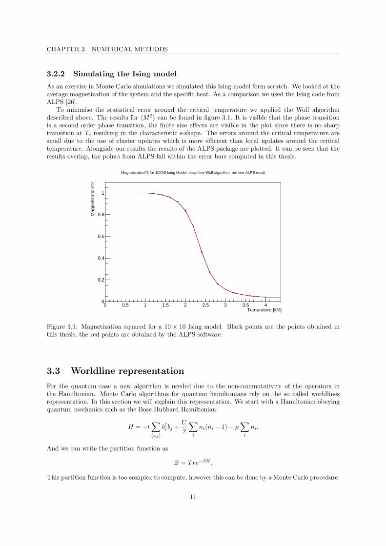
As an exercise in Monte Carlo simulations we simulated this Ising model form scratch. We looked at theaverage magnetization of the system and the specific heat. As a comparison we used the Ising code fromALPS [26].
To minimise the statistical error around the critical temperature we applied the Wolf algorithmdescribed above. The results for 〈M2〉 can be found in figure 3.1. It is visible that the phase transitionis a second order phase transition, the finite size effects are visible in the plot since there is no sharptransition at Tc resulting in the characteristic s-shape. The errors around the critical temperature aresmall due to the use of cluster updates which is more efficient than local updates around the criticaltemperature. Alongside our results the results of the ALPS package are plotted. It can be seen that theresults overlap, the points from ALPS fall within the error bars computed in this thesis.
Temprature [k/J]0 0.5 1 1.5 2 2.5 3 3.5 4
Mag
netiz
atio
n^2
0
0.2
0.4
0.6
0.8
1
Magnetization^2 for 10X10 Ising Model, black line Wolf algorithm, red line ALPS result
Figure 3.1: Magnetization squared for a 10 × 10 Ising model. Black points are the points obtained inthis thesis, the red points are obtained by the ALPS software.
3.3 Worldline representation
For the quantum case a new algorithm is needed due to the non-commutativity of the operators inthe Hamiltonian. Monte Carlo algorithms for quantum hamiltonians rely on the so called worldlinesrepresentation. In this section we will explain this representation. We start with a Hamiltonian obeyingquantum mechanics such as the Bose-Hubbard Hamiltonian:
H = −t∑〈i,j〉
b†i bj +U
2
∑i
ni(ni − 1)− µ∑i
ni.
And we can write the partition function as
Z = Tre−βH .
This partition function is too complex to compute, however this can be done by a Monte Carlo procedure.
11
CHAPTER 3. NUMERICAL METHODS
The core of the idea is that we map our d-dimensional quantum system on a (d+1)-dimensionalclassical system. To compute this partition function one starts by discretising the imaginary time bywriting it in M steps of ∆τ :
β → ∆τM,
Z = Tre−βH = Tre−(∆τH)M .
And the trace is written as a sum over the complete set of position eigenstates:
Z = Tre−(∆τH)M
=∑i
〈i|e−(∆τH)M |i〉. (3.8)
Furthermore, we write the exponent of the sum of M as a product of M exponentials and insert basisstates
∑i |i〉〈i| between all operators:
Z →∑
i1,...,iM
〈i1|e−∆τH |i2〉〈i2|e−∆τH |i3〉 . . . 〈iL|e−∆τH |i1〉
=∑i1...iM
P (i1, i2)P (i2, i3) . . . P (iM, i1).(3.9)
Here we make use of the Suzuki-Trotter approximation which becomes exact in the case of M → ∞ ,∆τ → 0. And the states |in〉 are the configurations of the bosons at imaginary time n, so it describeshow many particles are at each lattice site at imaginary time n. Under the operators e−∆τH the state|i1〉 evolves in imaginary time. Since in the Bose-Hubbard model the hopping term changes the stateby shifting only one particle to a neighbouring site, the sequence of matrix elements, 〈i|e−∆τH |j〉, iscompletely determined by the evolution of occupation numbers ni(τ). This can be viewed in the socalled worldlines interpretation as illustrated in figure 3.2. The values of P (i, j) can be interpreted asprobabilities.
Note that negative probabilities are in general not interpretable. So if off-diagonal values of thehamiltonian are positive these probabilities will be negative. (The emergence of the minus sign comesfrom positive off-diagonal values which can be seen from the approximation e−∆τH → 1−∆τH+O(τ2)).By taking account for a minus sign the algorithm slows down exponentially as O(eβN ) while without thesign problem the worldlines representation scales with O(βN). This is referred to as the negative signproblem. Examples of systems with positive off-diagonal values are frustrated spin systems. Anothersign problem occurs in fermionic systems where a minus sign occurs when two fermions exchange. Thisis the reason why Monte Carlo techniques don’t work for fermionic systems.
For each configuration a weight is assigned. Now the partition function can be computed usinga Monte Carlo algorithm. The aforementioned Metropolis algorithm is a possible candidate. In theworldlines representation the worldlines need to be continuous to give a valid physical system (due toparticle number conservation). Update moves that break worldlines are not be allowed.
This world line algorithm is derived for discrete time, in this thesis we use an algorithm which works inthe continues time limit. The main idea of the representation stays the same, only updates are proposedfor a certain time step instead at each discrete time.
3.3.1 The Worm algorithm
Single update methods like the Metropolis algorithm are not efficient because of the critical slowingdown near the critical temperature. There are other, more sophisticated, algorithms based on theKandel-Domany framework which does not have this problem. Algorithms include: the Loop Algorithm[28] and the Directed Loop Algorithm [29]. Another, more efficient, local update scheme is the WormAlgorithm [30], and the Directed Worm Algorithm [31]. This is the algorithm used in this thesis andwill be described in this section. The Worm Algorithm has two more advantages in comparison withmetropolis-like local updates. The first is that the worm algorithm is ergodic, since it includes moves
12
CHAPTER 3. NUMERICAL METHODS
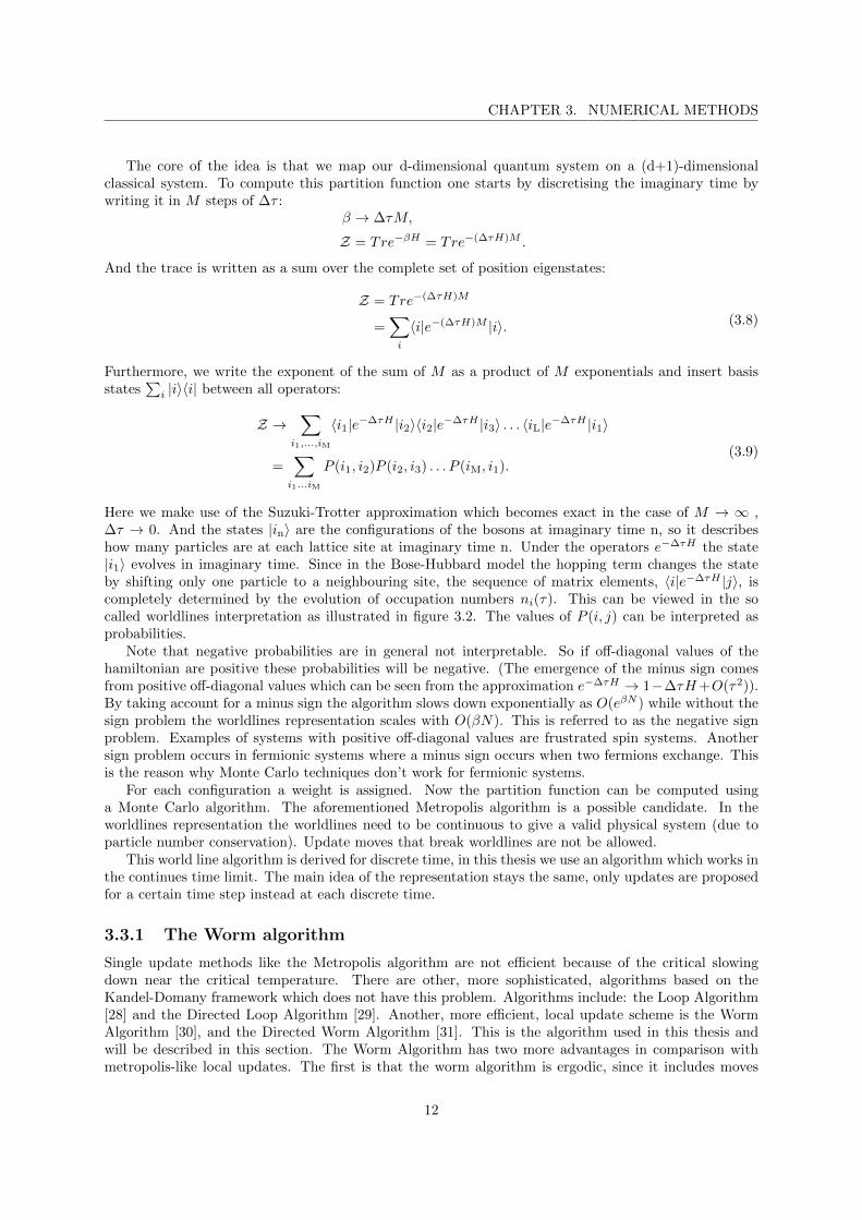
Figure 3.2: Example of a worldlines representation for a 1-dimensional lattice.The horizontal axis isdisplaying the lattice site, and the vertical axis the imaginary time direction. The number of lines oneach lattice site display the number of particles, so one line means one particle is present on that latticesite, two lines two particles, zero lines no particles and so forth. Note that each line has to be continuousto be a valid. At sites 5 and 6 a worm is inserted, where the red dot denotes the wormhead and the bluedot the wormtail. Figure obtained from [27]
13
CHAPTER 3. NUMERICAL METHODS
which can create particles winding over a periodic system. The second merit is that it is capable ofcomputing off-diagonal correlation functions such as the Green’s function.
The Worm Algorithm starts by inserting a segment of worldline in to a worldlines representation.This segment can either raise or lower (create or annihilate) the number of particles at that segment.This segment is called the worm. One of the end points of the worm stays immobile, this is called thewormtail, and the other end moves in the representation, this is called the wormhead. In figure 3.2 thereis an example of a worm at sites 5 and 6. The wormhead moves around until it reaches the wormtailsuch that a diagonal configuration is achieved and the update is completed.
Propagation of the wormhead can be described in continuous time, the wormhead jumps from τp toa new time τ ′p:
τ ′p − τp = − log(1− r)εp
.
Here r is a random number in the interval [0,1[ and εp the eigenvalue of the diagonal Hamiltonian partat state p. If in this jump the wormhead does not pass a vertex the wormhead either jumps at time τ+
ν
to a neighbouring site and creates a new vertex, or the worm turns around in its direction (this is calledbouncing). If the wormhead does pass a vertex in the jump the wormhead is halted and the followingthree scenarios can occur. One, the passed vertex is the wormtail, and the wormhead and the wormtailare connected such that there is a diagonal configuration and the update is completed. Two, if the vertexis of the same type, creating or annihilating, the worm crosses over with probability 1. Three, if thevertex is of the different type the wormhead either: jumps to the neighbouring site and deletes the vertexat time t+ν , jumps to the neighbouring site of its neighbouring site at time τ−ν and relinks the vertex,or changes its direction. If the worm still exists the algorithm continues propagating the wormhead byproposing a new jump from the new wormhead position. A more sophisticated algorithm, the DirectedWorm Algorithm, suppresses the bouncing leading to more efficient computations [32].
Worms can be seen as annihilation or creation operators, b(τ) b†(τ), which extend a configurationto an extended configuration of n vertices and the annihilation (creation) operator at time τp (τq). Theconfiguration weight is defined as
W = (e−τ1ε1Vi1i2eτ1ε2) . . . (e−τpεpbpe
τpε′p) . . . (e−τqεqb†pe
τqε′q ) . . . (e−τnεnVini1e
τnε1),
where Vij = 〈i|t∑〈i,j〉 b
†i bj |j〉 . This sums up to the greens function after normalisation
G =1
Z
∞∑m=0
∑i1...in
∑ip,iq
∫ β
0
dτ1 . . .
∫ τm−1
0
dτn(e−τ1ε1Vi1i2eτ1ε2) . . .
. . . (e−τpεpbpeτpε′p) . . . (e−τqεqb†pe
τqε′q ) . . . (e−τnεnVini1e
τnε1).
(3.10)
Density matrices are Greens functions at equal time: 〈b†pbq〉 = G(xp, τ ;xq, τ) [27].In this thesis the Directed Worm Algorithm implementation of the ALPS package is used [26]. For
some chapters in this thesis alterations to the lattice and local hamiltonian are made.
3.3.2 Observables
An observable in the worldlines representation can be computed in the following way:
〈O〉 =TrOe−βH
Z(3.11)
From here we can statistically estimate the expectation value 〈O〉. This can be computed by taking theaverage of different configurations x(i):
〈O〉 =1
N
N∑i=1
〈O(x(i))〉. (3.12)
14
CHAPTER 3. NUMERICAL METHODS
As mentioned before, the error on this expectation value is equation (3.2), which differs a factor 1√N
from a normal standard deviation.For some observables, improved, or more sophisticated estimators exist. Observables we like to give
extra attention are the (local) density and the superfluid stiffness in the Bose Hubbard model. The localdensity is computed by taking an average of the number of particles over imaginary time at each lattice.The total density can be computed by taking the average of all the local density values.
The superfluid stiffness can be computed from the winding number as:
ρs =mT
2〈W2〉. (3.13)
Here m is the boson mass and W the winding number [33, 34]. The winding number denotes the numberof times the particles wind over the cyclic boundary conditions. The superfluid stiffness and superfluiddensity are related as ns = ρsm, where I denoted the superfluid density as ns and m is the boson mass[35]. In literature both quantities are often denoted as ρs. In this thesis we will use ρs for the superfluidstiffness as a default, except when mentioned otherwise.
15
Chapter 4
Normal fluid to superfluid phasetransition
4.1 Normal to superfluid
In this chapter the phase transition between the normal fluid and the superfluid phase in the Bose-Hubbard model is investigated, this phase transition is a BKT-phase transition. We looked at the phasediagram of this transition and determined the critical temperature for different values of U
t at fillingn = 1. First we treat the method used to determine this critical temperature, after which we compareour results to known results from literature. Finally we determine the critical temperature for theKagome lattice the latter has not been done before.
4.2 Method
The method used to find the critical temperature TKT of the BKT-transition has been used before inseveral other papers [34, 36, 37, 38] and makes use of the Nelson-Kosterlitz relation which we derived insection 2.3.1:
ρs(TKT) =2
πmTKT, (4.1)
where ρs is the superfluid stiffness and m the boson mass [18]. This relation predicts that the superfluidstiffness jumps from zero to this value from equation (4.1) at the critical temperature. For finite sizesthe correction ρsπ = 2mTKT(1 + {2Log[ L
L0(TKT) )]}−1) is given [33]. A plot of the superfluid stiffness at
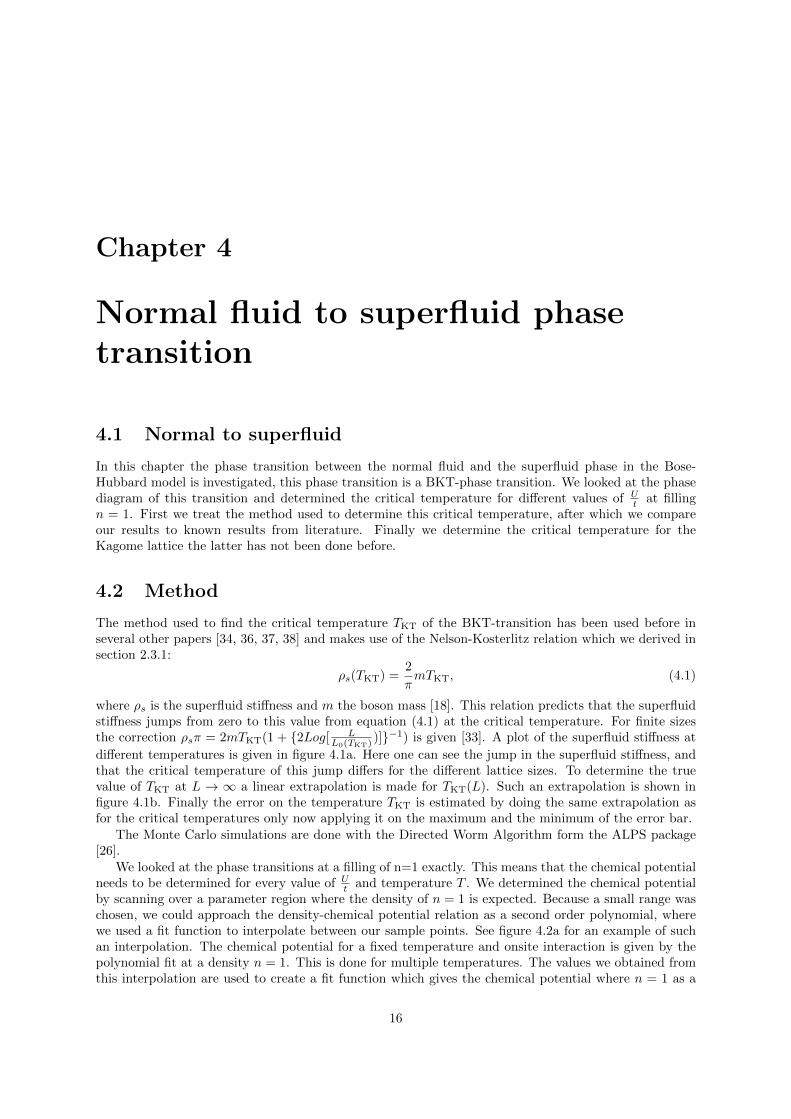
different temperatures is given in figure 4.1a. Here one can see the jump in the superfluid stiffness, andthat the critical temperature of this jump differs for the different lattice sizes. To determine the truevalue of TKT at L → ∞ a linear extrapolation is made for TKT(L). Such an extrapolation is shown infigure 4.1b. Finally the error on the temperature TKT is estimated by doing the same extrapolation asfor the critical temperatures only now applying it on the maximum and the minimum of the error bar.
The Monte Carlo simulations are done with the Directed Worm Algorithm form the ALPS package[26].
We looked at the phase transitions at a filling of n=1 exactly. This means that the chemical potentialneeds to be determined for every value of U
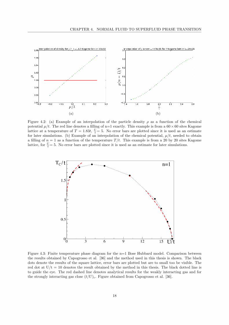
t and temperature T . We determined the chemical potentialby scanning over a parameter region where the density of n = 1 is expected. Because a small range waschosen, we could approach the density-chemical potential relation as a second order polynomial, wherewe used a fit function to interpolate between our sample points. See figure 4.2a for an example of suchan interpolation. The chemical potential for a fixed temperature and onsite interaction is given by thepolynomial fit at a density n = 1. This is done for multiple temperatures. The values we obtained fromthis interpolation are used to create a fit function which gives the chemical potential where n = 1 as a
16
CHAPTER 4. NORMAL FLUID TO SUPERFLUID PHASE TRANSITION
0.8 1.0 1.2 1.4 1.6 1.8 2.0 2.2 2.4Tt
0.0
0.2
0.4
0.6
0.8
1.0
1.2
1.4
1.6
ρs
Stiffness for square lattice, u/t=10
2πTt
20 x 2030 x 3040 x 4050 x 5060 x 60
(a)
0.00 0.01 0.02 0.03 0.04 0.05 0.06 0.07 0.081/L
1.35
1.40
1.45
1.50
1.55
1.60
1.65
Tc/
t
Fit for Tc versus L, L->∞ = 1.40601436914=/-0.00697677655292Tc/t
Fit a*x + bData points
(b)
Figure 4.1: (a) Superfluid stiffness as a function of Tt for a square lattice with onsite interaction U
t = 10and a filling of n = 1. Different lattice sizes are plotted to demonstrate the finite size effect. Theyellow dotted line denotes the value of the Nelson-Kosterlitz relation, the intersection gives the criticaltemperature for each lattice size. (b) Critical temperatures obtained from the Nelson-Kosterlitz relationin figure 4.1a. The blue dotted line denotes the extrapolation of the critical temperature to infinitesystem size. This results in limL→∞ Tc(L) = 1.603(7)
function of the temperature µ(T ) → (n = 1) which is used to set the chemical potential for the finalsimulations. See figure 4.2b for the temperature interpolation.
4.3 Simulations
4.3.1 Literature comparison
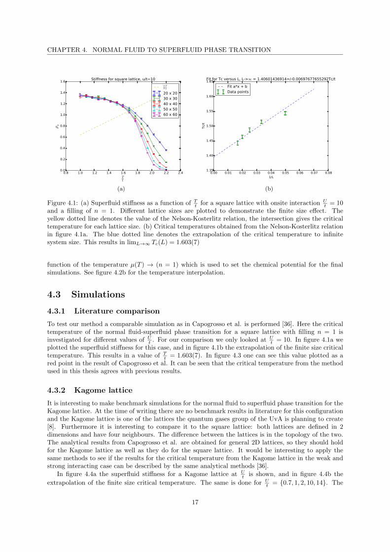
To test our method a comparable simulation as in Capogrosso et al. is performed [36]. Here the criticaltemperature of the normal fluid-superfluid phase transition for a square lattice with filling n = 1 isinvestigated for different values of U
t . For our comparison we only looked at Ut = 10. In figure 4.1a we
plotted the superfluid stiffness for this case, and in figure 4.1b the extrapolation of the finite size criticaltemperature. This results in a value of T
t = 1.603(7). In figure 4.3 one can see this value plotted as ared point in the result of Capogrosso et al. It can be seen that the critical temperature from the methodused in this thesis agrees with previous results.
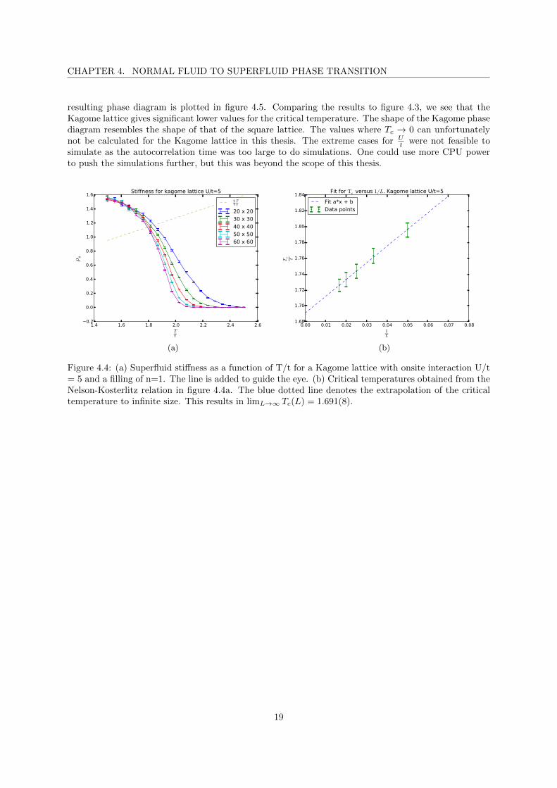
4.3.2 Kagome lattice
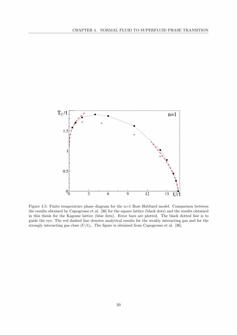
It is interesting to make benchmark simulations for the normal fluid to superfluid phase transition for theKagome lattice. At the time of writing there are no benchmark results in literature for this configurationand the Kagome lattice is one of the lattices the quantum gases group of the UvA is planning to create[8]. Furthermore it is interesting to compare it to the square lattice: both lattices are defined in 2dimensions and have four neighbours. The difference between the lattices is in the topology of the two.The analytical results from Capogrosso et al. are obtained for general 2D lattices, so they should holdfor the Kagome lattice as well as they do for the square lattice. It would be interesting to apply thesame methods to see if the results for the critical temperature from the Kagome lattice in the weak andstrong interacting case can be described by the same analytical methods [36].
In figure 4.4a the superfluid stiffness for a Kagome lattice at Ut is shown, and in figure 4.4b the
extrapolation of the finite size critical temperature. The same is done for Ut = {0.7, 1, 2, 10, 14}. The
17
CHAPTER 4. NORMAL FLUID TO SUPERFLUID PHASE TRANSITION
(a) (b)
Figure 4.2: (a) Example of an interpolation of the particle density ρ as a function of the chemicalpotential µ/t. The red line denotes a filling of n=1 exactly. This example is from a 60×60 sites Kagomelattice at a temperature of T = 1.83t, U
t = 5. No error bars are plotted since it is used as an estimatefor later simulations. (b) Example of an interpolation of the chemical potential, µ/t, needed to obtaina filling of n = 1 as a function of the temperature T/t. This example is from a 20 by 20 sites Kagomelattice, for U
t = 5. No error bars are plotted since it is used as an estimate for later simulations.
t
t
Figure 4.3: Finite temperature phase diagram for the n=1 Bose Hubbard model. Comparison betweenthe results obtained by Capogrosso et al. [36] and the method used in this thesis is shown. The blackdots denote the results of the square lattice, error bars are plotted but are to small too be visible. Thered dot at U/t = 10 denotes the result obtained by the method in this thesis. The black dotted line isto guide the eye. The red dashed line denotes analytical results for the weakly interacting gas and forthe strongly interacting gas close (t/U)c. Figure obtained from Capogrosso et al. [36].
18
CHAPTER 4. NORMAL FLUID TO SUPERFLUID PHASE TRANSITION
resulting phase diagram is plotted in figure 4.5. Comparing the results to figure 4.3, we see that theKagome lattice gives significant lower values for the critical temperature. The shape of the Kagome phasediagram resembles the shape of that of the square lattice. The values where Tc → 0 can unfortunatelynot be calculated for the Kagome lattice in this thesis. The extreme cases for U
t were not feasible tosimulate as the autocorrelation time was too large to do simulations. One could use more CPU powerto push the simulations further, but this was beyond the scope of this thesis.
1.4 1.6 1.8 2.0 2.2 2.4 2.6Tt
0.2
0.0
0.2
0.4
0.6
0.8
1.0
1.2
1.4
1.6
ρs
Stiffness for kagome lattice U/t=5
2πTt
20 x 2030 x 3040 x 4050 x 5060 x 60
(a)
0.00 0.01 0.02 0.03 0.04 0.05 0.06 0.07 0.081L
1.68
1.70
1.72
1.74
1.76
1.78
1.80
1.82
1.84
Tc t
Fit for Tc versus 1/L. Kagome lattice U/t=5
Fit a*x + bData points
(b)
Figure 4.4: (a) Superfluid stiffness as a function of T/t for a Kagome lattice with onsite interaction U/t= 5 and a filling of n=1. The line is added to guide the eye. (b) Critical temperatures obtained from theNelson-Kosterlitz relation in figure 4.4a. The blue dotted line denotes the extrapolation of the criticaltemperature to infinite size. This results in limL→∞ Tc(L) = 1.691(8).
19
CHAPTER 4. NORMAL FLUID TO SUPERFLUID PHASE TRANSITION
t
t
Figure 4.5: Finite temperature phase diagram for the n=1 Bose Hubbard model. Comparison betweenthe results obtained by Capogrosso et al. [36] for the square lattice (black dots) and the results obtainedin this thesis for the Kagome lattice (blue dots). Error bars are plotted. The black dotted line is toguide the eye. The red dashed line denotes analytical results for the weakly interacting gas and for thestrongly interacting gas close (U/t)c. The figure is obtained from Capogrosso et al. [36].
20
Chapter 5
Mott-superfluid phase transition
5.1 Method
In this chapter the occupation ρ and superfluid density ρs as a function of the chemical potential in theBose-Hubbard model is examined. Several plots for a fixed temperature T and different hopping t
U aremade.
To ensure that the simulations are in the same region for the temperature and the hopping-onsiteinteraction ratio t
U as the experiments an estimation is made. Doing actual band structure calculationsto extract the hopping and onsite interaction for our geometries was outside of the scope of this thesis.To make an estimate of those values we followed the results of Gerbier et al. [39]. They calculated theband structure for the cubic lattice and found the following approximate expressions for the hopping andonsite interaction, respectively:
t
ER= 1.42
(V0
ER
)0.98
e−2.07√V0/ER ,
U
ER=
5.97asλ
(V0
ER
)0.88
.
(5.1)
Here ER is the recoil energy, V0 the lattice depth and as the lattice spacing. These formulas were foundto be accurate within 1% in the range V0 = 8− 30ER. Although it is not possible to compare the bandstructures of the cubic lattice to the band structures of the Kagome and triangular lattices but it givesan idea of which magnitudes the experiments are dealing with.
To do a crosscheck for equation (5.1) in the Kagome lattice we did an approximation off the Wannierfunctions in the magnetic potential of the quantum gases and quantum information group at the UvA[8]. As mentioned in section 2.1.2 the Wannier function can be approximated by a gaussian function as:
w(x−Rn) =
(1
πaax
)1/4
e− (x−Rn)2
2a2ax , (5.2)
where aax =√
~mωax
, and ωax the harmonic oscillator length in the axial direction [9]. By using the
lattice potential we found for a Kagome lattice with a spacing of 100nm and lattice to atoms spacing150nm that the hopping would be t = 27nK. This lattice to atoms spacing gives a V0
ER= 1.774 which
results in t = 145nK according to equation (5.1). Note that both methods are approximations. Wecan conclude that it is justified to use equation (5.1) to estimate the magnitudes of the Bose-Hubbardparameters in the experiment.
The temperature of the experiment is in the range 0.2µK−2µK. Using equation (5.1) the temperaturecan be expressed in units of hopping, t.
21
CHAPTER 5. MOTT-SUPERFLUID PHASE TRANSITION
5.2 Result
5.2.1 Literature comparison and finite temperature and finite size effects
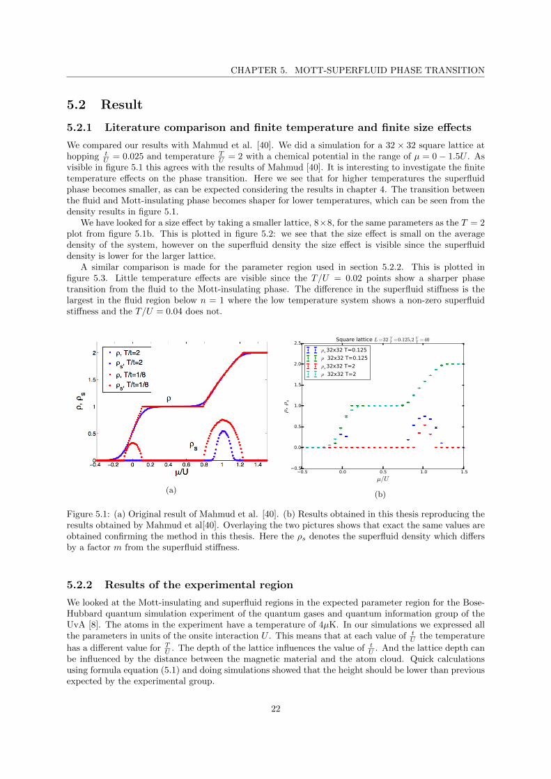
We compared our results with Mahmud et al. [40]. We did a simulation for a 32 × 32 square lattice athopping t
U = 0.025 and temperature TU = 2 with a chemical potential in the range of µ = 0− 1.5U . As
visible in figure 5.1 this agrees with the results of Mahmud [40]. It is interesting to investigate the finitetemperature effects on the phase transition. Here we see that for higher temperatures the superfluidphase becomes smaller, as can be expected considering the results in chapter 4. The transition betweenthe fluid and Mott-insulating phase becomes shaper for lower temperatures, which can be seen from thedensity results in figure 5.1.
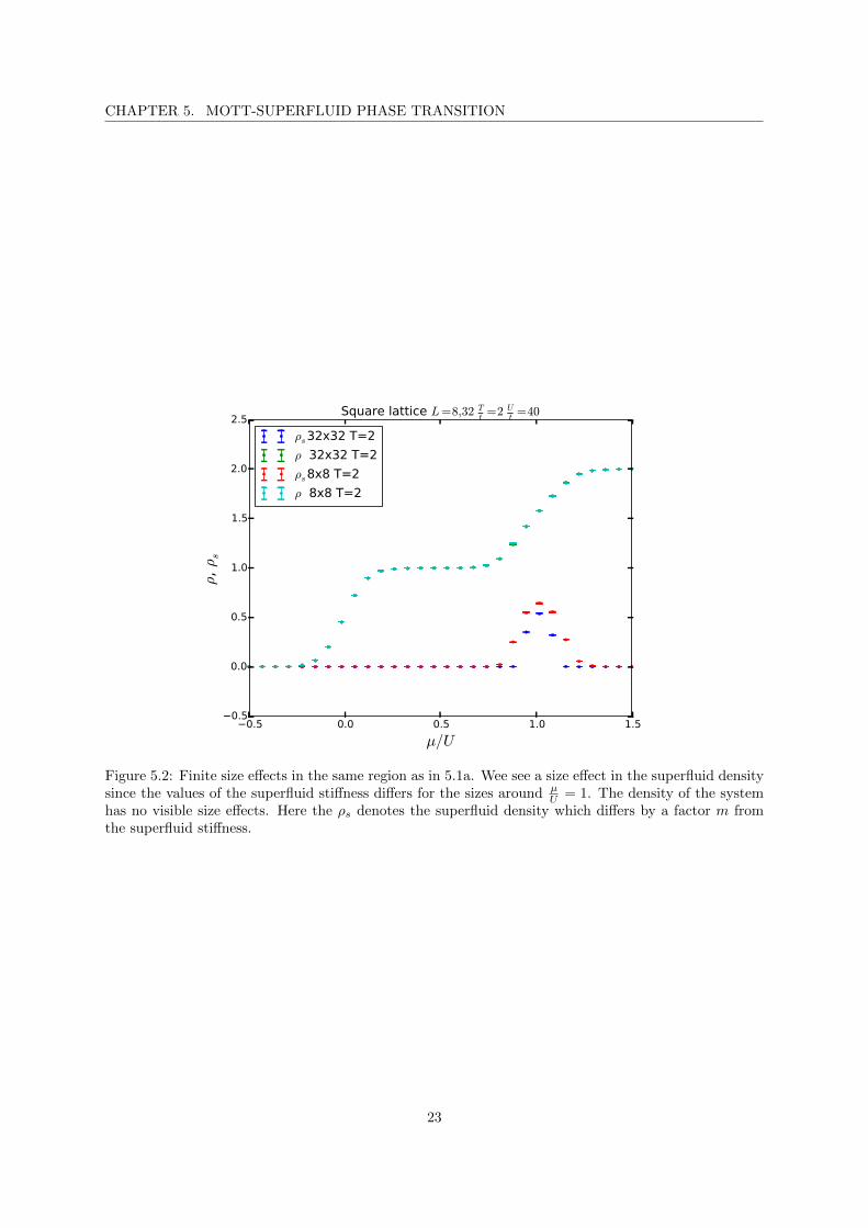
We have looked for a size effect by taking a smaller lattice, 8×8, for the same parameters as the T = 2plot from figure 5.1b. This is plotted in figure 5.2: we see that the size effect is small on the averagedensity of the system, however on the superfluid density the size effect is visible since the superfluiddensity is lower for the larger lattice.
A similar comparison is made for the parameter region used in section 5.2.2. This is plotted infigure 5.3. Little temperature effects are visible since the T/U = 0.02 points show a sharper phasetransition from the fluid to the Mott-insulating phase. The difference in the superfluid stiffness is thelargest in the fluid region below n = 1 where the low temperature system shows a non-zero superfluidstiffness and the T/U = 0.04 does not.
(a)
0.5 0.0 0.5 1.0 1.5
µ/U
0.5
0.0
0.5
1.0
1.5
2.0
2.5
ρ, ρs
Square lattice L=32 Tt=0.125,2 U
t=40
ρs32x32 T=0.125
ρ 32x32 T=0.125
ρs32x32 T=2
ρ 32x32 T=2
(b)
Figure 5.1: (a) Original result of Mahmud et al. [40]. (b) Results obtained in this thesis reproducing theresults obtained by Mahmud et al[40]. Overlaying the two pictures shows that exact the same values areobtained confirming the method in this thesis. Here the ρs denotes the superfluid density which differsby a factor m from the superfluid stiffness.
5.2.2 Results of the experimental region
We looked at the Mott-insulating and superfluid regions in the expected parameter region for the Bose-Hubbard quantum simulation experiment of the quantum gases and quantum information group of theUvA [8]. The atoms in the experiment have a temperature of 4µK. In our simulations we expressed allthe parameters in units of the onsite interaction U . This means that at each value of t
U the temperature
has a different value for TU . The depth of the lattice influences the value of t
U . And the lattice depth canbe influenced by the distance between the magnetic material and the atom cloud. Quick calculationsusing formula equation (5.1) and doing simulations showed that the height should be lower than previousexpected by the experimental group.
22
CHAPTER 5. MOTT-SUPERFLUID PHASE TRANSITION
0.5 0.0 0.5 1.0 1.5
µ/U
0.5
0.0
0.5
1.0
1.5
2.0
2.5
ρ, ρs
Square lattice L=8,32 Tt=2 U
t=40
ρs32x32 T=2
ρ 32x32 T=2
ρs8x8 T=2
ρ 8x8 T=2
Figure 5.2: Finite size effects in the same region as in 5.1a. Wee see a size effect in the superfluid densitysince the values of the superfluid stiffness differs for the sizes around µ
U = 1. The density of the systemhas no visible size effects. Here the ρs denotes the superfluid density which differs by a factor m fromthe superfluid stiffness.
23
CHAPTER 5. MOTT-SUPERFLUID PHASE TRANSITION
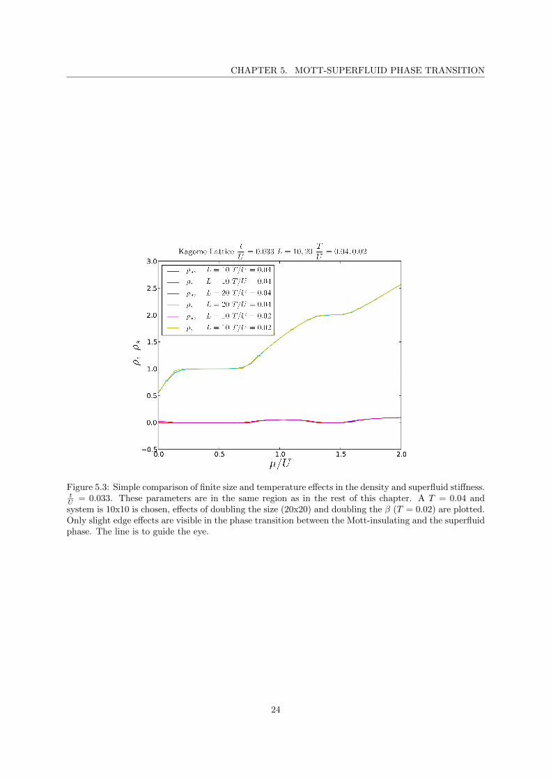
Figure 5.3: Simple comparison of finite size and temperature effects in the density and superfluid stiffness.tU = 0.033. These parameters are in the same region as in the rest of this chapter. A T = 0.04 andsystem is 10x10 is chosen, effects of doubling the size (20x20) and doubling the β (T = 0.02) are plotted.Only slight edge effects are visible in the phase transition between the Mott-insulating and the superfluidphase. The line is to guide the eye.
24
CHAPTER 5. MOTT-SUPERFLUID PHASE TRANSITION
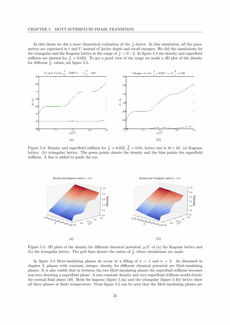
In this thesis we did a more theoretical evaluation of the tU -factor. In this simulation, all the para-
meters are expressed in t and U instead of lattice depth and recoil energies. We did the simulations forthe triangular and the Kagome lattice in the range of t
U = 0− 2. In figure 5.4 the density and superfluidstiffness are plotted for t
U = 0.022. To get a good view of the range we made a 3D plot of the densityfor different t
U values, see figure 5.5.
(a) (b)
Figure 5.4: Density and superfluid stiffness for tU = 0.022, T
U = 0.04, lattice size is 10× 10. (a) Kagomelattice. (b) triangular lattice. The green points denote the density and the blue points the superfluidstiffness. A line is added to guide the eye.
tU
0.020.04
0.060.08
0.100.12
0.14
µ/U0.0
0.51.0
1.52.0
Densi
ty
0.5
1.0
1.5
2.0
2.5
3.0
Density plot Kagome Lattice TU
=0.04
(a)
tU 0.000.020.040.060.080.100.120.14
µ/U0.0
0.51.0
1.52.0
Densi
ty
0.5
1.0
1.5
2.0
2.5
3.0
3.5
Density plot Triangular Lattice TU
=0.04
(b)
Figure 5.5: 3D plots of the density for different chemical potential, µ/U of (a) the Kagome lattice and(b) the triangular lattice. The grid lines denote the values of t
U where simulations are made.
In figure 5.4 Mott-insulating phases do occur at a filling of n = 1 and n = 2. As discussed inchapter 2, phases with constant, integer, density for different chemical potential are Mott-insulatingphases. It is also visible that in between the two Mott-insulating phases the superfluid stiffness becomesnon-zero denoting a superfluid phase. A non constant density and zero superfluid stiffness would denotethe normal fluid phase [40]. Both the kagome (figure 5.4a) and the triangular (figure 5.4b) lattice showall three phases at finite temperature. From figure 5.5 can be seen that the Mott-insulating phases are
25
CHAPTER 5. MOTT-SUPERFLUID PHASE TRANSITION
smaller in the triangular lattice case than in the Kagome lattice case. In the triangular lattice the n = 2Mott lobe seems to finish around t
U = 0.03, while in the Kagome lattice case this is at tU = 0.05. The
tip of the n = 1 Mott lobe seems to be at tU = 0.05, while in the Kagome lattice case this is at t
U = 0.07.
26
Chapter 6
Superlattices
6.1 Introduction
An interest of the quantum gasses and quantum information group is to investigate the Bose-Hubbardmodel in different geometries, like the Kagome and the triangular geometry. This Kagome geometry iscreated on top of a triangular lattice by raising the bottom magnetic field at certain lattice sites. Theraised magnetic field repels atoms from this lattice site. To fully resemble a Kagome lattice the raisingneeds to be sufficient. If it is too low atoms still occupy this lattice site, if it is too high the local magneticfield of neighbouring lattice sites can be affected. In this chapter the influence of this local magnetic fieldraising on the triangular lattice is investigated. A combination of two lattices is called a superlattice.
In our simulation we simulate this effect by raising the local chemical potential. First let us remindthe Bose-Hubbard hamiltonian:
H = −t∑〈i,j〉
b†i bj +U
2
∑i
ni(ni − 1)−∑i
µini. (6.1)
Where we made a slight alteration from equation (2.10) by writing a local chemical potential instead ofa general one. For this local chemical potential we write:
µi =
{µ Kagome sites
µ− δ non-Kagome sites. (6.2)
Here δ is the magnitude of offset for the raised lattice sites, Kagome sites are the sites which are partof the Kagome geometry and non-Kagome sites are the sites which are not and are raised by a value ofδ. The simulation is done with use of the directed worm algorithm provided by the ALPS project [26].The author implemented equation (6.2) into the DWA code.
6.2 Results
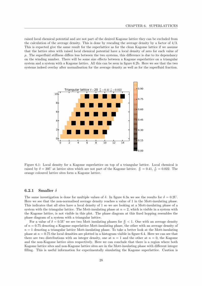
The influence of different values of δ on a system with a triangular lattice is investigated. As a startwe looked at a very large δ to see if we get a pure Kagome geometry. We took δ = 20U for a chemicalpotential of µ = 0.41U . This can be seen in figure 6.1. There it is visible that the occupation of thelattice sites with raised local chemical potential have a local density of 0, and the other lattice sites havea non zero occupation. A Kagome lattice can be drawn over the orange coloured lattice sites in figure 6.1.
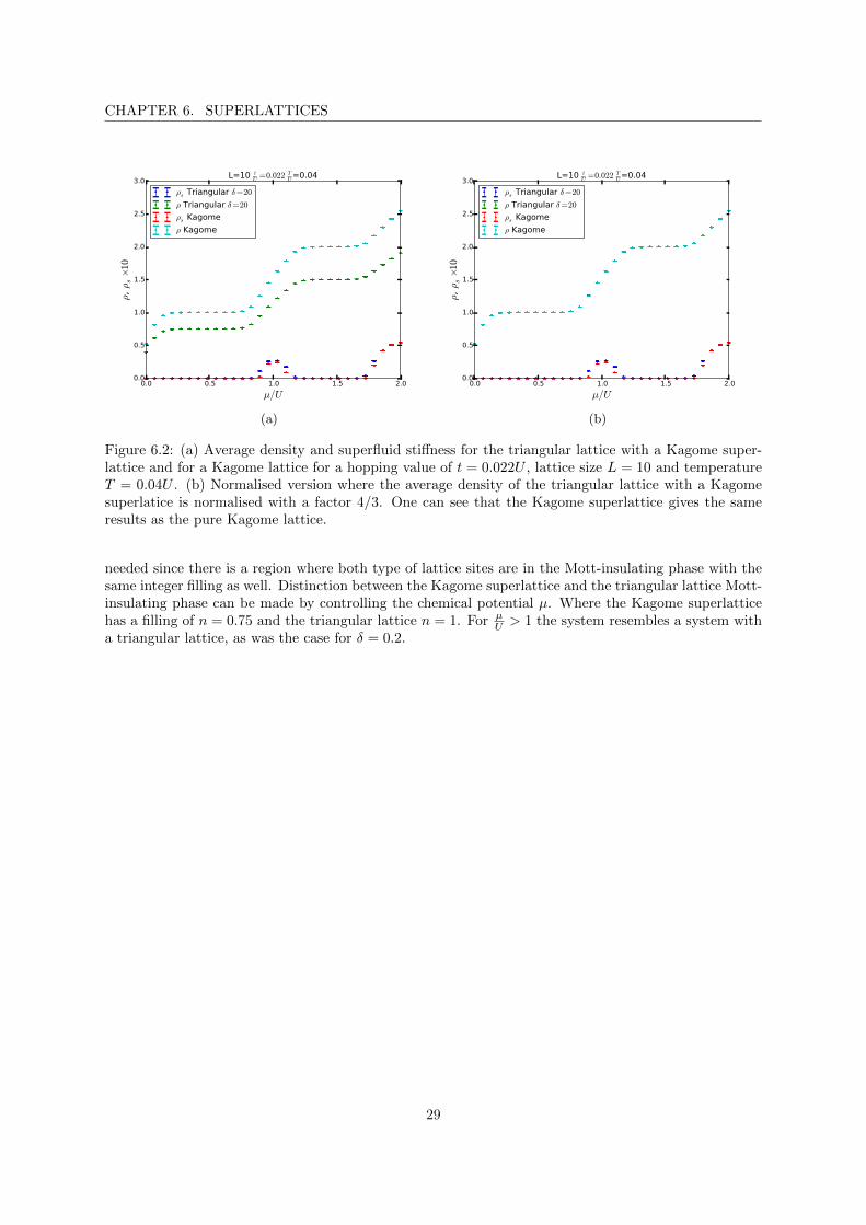
To compare the results of a superlattice with δ = 20U to a pure Kagome lattice we compared thetotal density and superfluid on a range of the total chemical potential µ = 0 − 2. This can be seen infigure 6.2a. Here you can see that both systems have the same phases for the same chemical potential.To make a better comparison we can normalise the superlattice. Since 1/4th of the lattice sites has a
27
CHAPTER 6. SUPERLATTICES
raised local chemical potential and are not part of the desired Kagome lattice they can be excluded fromthe calculation of the average density. This is done by rescaling the average density by a factor of 4/3.This is expected give the same result for the superlattice as for the clean Kagome lattice if we assumethat the lattice sites with raised local chemical potential have a local density of zero for each value ofµ. The superfluid stiffness differs less between the two systems, this difference is due to its dependancyon the winding number. There will be some size effects between a Kagome superlattice on a triangularsystem and a system with a Kagome lattice. All this can be seen in figure 6.2b. Here we see that the twosystems indeed overlay after normalisation for the average density as well as for the superfluid fraction.
0 2 4 6 8 10 12 14
0
2
4
6
8
10
Triangular lattice δ=20 µU
=0.41 tU
=0.022
0.00
0.15
0.30
0.45
0.60
0.75
0.90
Figure 6.1: Local density for a Kagome superlattice on top of a triangular lattice. Local chemical israised by δ = 20U at lattice sites which are not part of the Kagome lattice. µ
U = 0.41, tU = 0.022. The
orange coloured lattice sites form a Kagome lattice.
6.2.1 Smaller δ
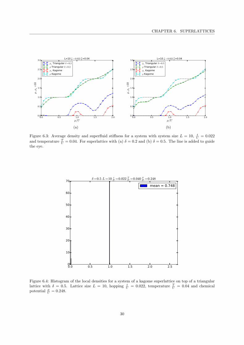
The same investigation is done for multiple values of δ. In figure 6.3a we see the results for δ = 0.2U .Here we see that the non-normalised average density reaches a value of 1 in the Mott-insulating phase.This indicates that all sites have a local density of 1 so we are looking at a Mott-insulating phase of asystem with the triangular lattice. The Mott-insulating phase at n = 2, which is visible in a system withthe Kagome lattice, is not visible in this plot. The phase diagram at this fixed hopping resembles thephase diagram of a system with a triangular lattice.
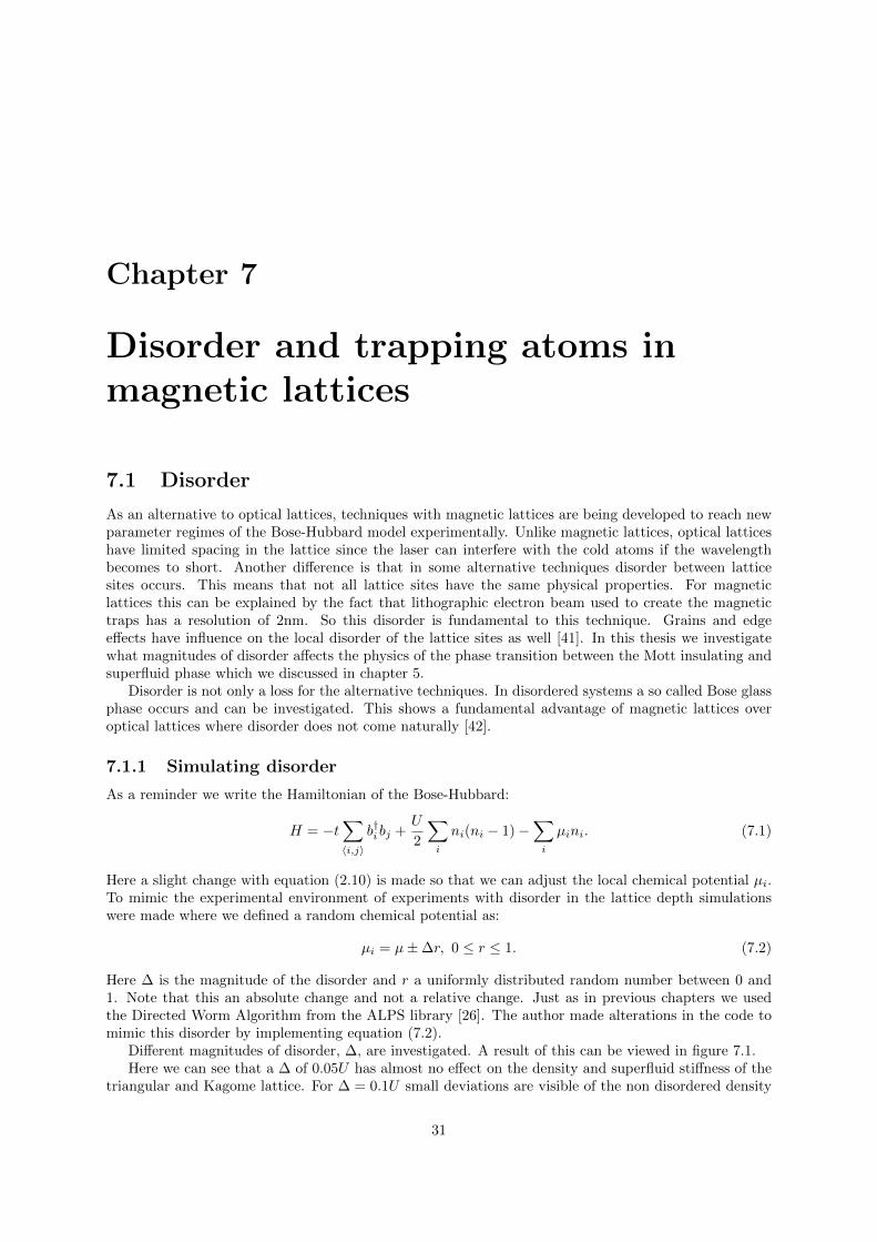
For a value of δ = 0.5U we see two Mott insulating phases for µU < 1. One with an average density
of n = 0.75 denoting a Kagome superlattice Mott-insulating phase, the other with an average density ofn = 1 denoting a triangular lattice Mott-insulating phase. To take a better look at the Mott-insulatingphase at n = 0.75 the local densities are plotted in a histogram visible in figure 6.4. Here we can see thatthere are two distributions with an integer density, one at n = 1 and the other at n = 0, the Kagomeand the non-Kagome lattice sites respectively. Here we can conclude that there is a region where bothKagome lattice sites and non-Kagome lattice sites are in the Mott-insulating phase with different integerfilling. This is useful information for experimentally simulating the Kagome superlattice. Caution is
28
CHAPTER 6. SUPERLATTICES
0.0 0.5 1.0 1.5 2.0
µ/U
0.0
0.5
1.0
1.5
2.0
2.5
3.0
ρ, ρs×1
0
L=10 tU
=0.022 TU=0.04
ρs Triangular δ=20
ρ Triangular δ=20
ρs Kagome
ρ Kagome
(a)
0.0 0.5 1.0 1.5 2.0
µ/U
0.0
0.5
1.0
1.5
2.0
2.5
3.0
ρ, ρs×1
0
L=10 tU
=0.022 TU=0.04
ρs Triangular δ=20
ρ Triangular δ=20
ρs Kagome
ρ Kagome
(b)
Figure 6.2: (a) Average density and superfluid stiffness for the triangular lattice with a Kagome super-lattice and for a Kagome lattice for a hopping value of t = 0.022U , lattice size L = 10 and temperatureT = 0.04U . (b) Normalised version where the average density of the triangular lattice with a Kagomesuperlatice is normalised with a factor 4/3. One can see that the Kagome superlattice gives the sameresults as the pure Kagome lattice.
needed since there is a region where both type of lattice sites are in the Mott-insulating phase with thesame integer filling as well. Distinction between the Kagome superlattice and the triangular lattice Mott-insulating phase can be made by controlling the chemical potential µ. Where the Kagome superlatticehas a filling of n = 0.75 and the triangular lattice n = 1. For µ
U > 1 the system resembles a system witha triangular lattice, as was the case for δ = 0.2.
29
CHAPTER 6. SUPERLATTICES
0.0 0.5 1.0 1.5 2.0
µ/U
0.0
0.5
1.0
1.5
2.0
2.5
3.0
ρ, ρs×1
0
L=10 tU
=0.022 TU=0.04
ρs Triangular δ=0.2
ρ Triangular δ=0.2
ρs Kagome
ρ Kagome
(a)
0.0 0.5 1.0 1.5 2.0
µ/U
0.0
0.5
1.0
1.5
2.0
2.5
3.0
ρ, ρs×1
0
L=10 tU
=0.022 TU=0.04
ρs Triangular δ=0.5
ρ Triangular δ=0.5
ρs Kagome
ρ Kagome
(b)
Figure 6.3: Average density and superfluid stiffness for a system with system size L = 10, tU = 0.022
and temperature TU = 0.04. For superlattice with (a) δ = 0.2 and (b) δ = 0.5. The line is added to guide
the eye.
0.0 0.5 1.0 1.5 2.0 2.50
10
20
30
40
50
60
70δ=0.5 L=10 t
U=0.022 T
U=0.040 µ
U=0.248
mean = 0.748
Figure 6.4: Histogram of the local densities for a system of a kagome superlattice on top of a triangularlattice with δ = 0.5. Lattice size L = 10, hopping t
U = 0.022, temperature TU = 0.04 and chemical
potential µU = 0.248.
30
Chapter 7
Disorder and trapping atoms inmagnetic lattices
7.1 Disorder
As an alternative to optical lattices, techniques with magnetic lattices are being developed to reach newparameter regimes of the Bose-Hubbard model experimentally. Unlike magnetic lattices, optical latticeshave limited spacing in the lattice since the laser can interfere with the cold atoms if the wavelengthbecomes to short. Another difference is that in some alternative techniques disorder between latticesites occurs. This means that not all lattice sites have the same physical properties. For magneticlattices this can be explained by the fact that lithographic electron beam used to create the magnetictraps has a resolution of 2nm. So this disorder is fundamental to this technique. Grains and edgeeffects have influence on the local disorder of the lattice sites as well [41]. In this thesis we investigatewhat magnitudes of disorder affects the physics of the phase transition between the Mott insulating andsuperfluid phase which we discussed in chapter 5.
Disorder is not only a loss for the alternative techniques. In disordered systems a so called Bose glassphase occurs and can be investigated. This shows a fundamental advantage of magnetic lattices overoptical lattices where disorder does not come naturally [42].
7.1.1 Simulating disorder
As a reminder we write the Hamiltonian of the Bose-Hubbard:
H = −t∑〈i,j〉
b†i bj +U
2
∑i
ni(ni − 1)−∑i
µini. (7.1)
Here a slight change with equation (2.10) is made so that we can adjust the local chemical potential µi.To mimic the experimental environment of experiments with disorder in the lattice depth simulationswere made where we defined a random chemical potential as:
µi = µ±∆r, 0 ≤ r ≤ 1. (7.2)
Here ∆ is the magnitude of the disorder and r a uniformly distributed random number between 0 and1. Note that this an absolute change and not a relative change. Just as in previous chapters we usedthe Directed Worm Algorithm from the ALPS library [26]. The author made alterations in the code tomimic this disorder by implementing equation (7.2).
Different magnitudes of disorder, ∆, are investigated. A result of this can be viewed in figure 7.1.Here we can see that a ∆ of 0.05U has almost no effect on the density and superfluid stiffness of the
triangular and Kagome lattice. For ∆ = 0.1U small deviations are visible of the non disordered density
31
CHAPTER 7. DISORDER AND TRAPPING ATOMS IN MAGNETIC LATTICES
(a) Triangular (b) Kagome
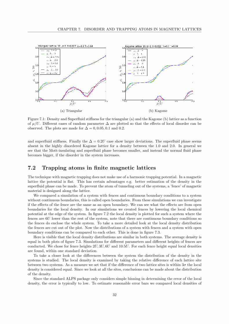
Figure 7.1: Density and Superfluid stiffness for the triangular (a) and the Kagome (b) lattice as a functionof µ/U . Different cases of random parameter ∆ are plotted so that the effects of local disorder can beobserved. The plots are made for ∆ = 0, 0.05, 0.1 and 0.2.
and superfluid stiffness. Finally the ∆ = 0.2U case show larger deviations. The superfluid phase seemsabsent in the highly disordered Kagome lattice for a density between the 1.0 and 2.0. In general wesee that the Mott-insulating and superfluid phase becomes smaller, and instead the normal fluid phasebecomes bigger, if the disorder in the system increases.
7.2 Trapping atoms in finite magnetic lattices
The technique with magnetic trapping does not make use of a harmonic trapping potential. In a magneticlattice the potential is flat. This has certain advantages e.g. better estimation of the density in thesuperfluid phase can be made. To prevent the atom of tunneling out of the systems, a ’fence’ of magneticmaterial is designed along the lattice.
We compared a simulation of a system with fences and continuous boundary conditions to a systemwithout continuous boundaries, this is called open boundaries. From these simulations we can investigateif the effects of the fence are the same as an open boundary. We can see what the effects are from openboundaries for the local density. In our simulations we created fences by lowering the local chemicalpotential at the edge of the system. In figure 7.2 the local density is plotted for such a system where thefences are 6U lower than the rest of the system, note that there are continuous boundary conditions sothe fences do enclose the whole system. To take a more detailed look at the local density distributionthe fences are cut out of the plot. Now the distributions of a system with fences and a system with openboundary conditions can be compared to each other. This is done in figure 7.3.
Here is visible that the local density distributions are similar in both systems. The average density isequal in both plots of figure 7.3. Simulations for different parameters and different heights of fences areconducted. We chose for fence heights 2U, 3U, 6U and 10.5U . For each fence height equal local densitiesare found, within one standard deviation.
To take a closer look at the differences between the system the distribution of the density in thesystems is studied. The local density is examined by taking the relative difference of each lattice sitebetween two systems. As a measure we set that if the difference of two lattice sites is within 3σ the localdensity is considered equal. Since we look at all the sites, conclusions can be made about the distributionof the density.
Since the standard ALPS package only considers simple binning in determining the error of the localdensity, the error is typically to low. To estimate reasonable error bars we compared local densities of
32
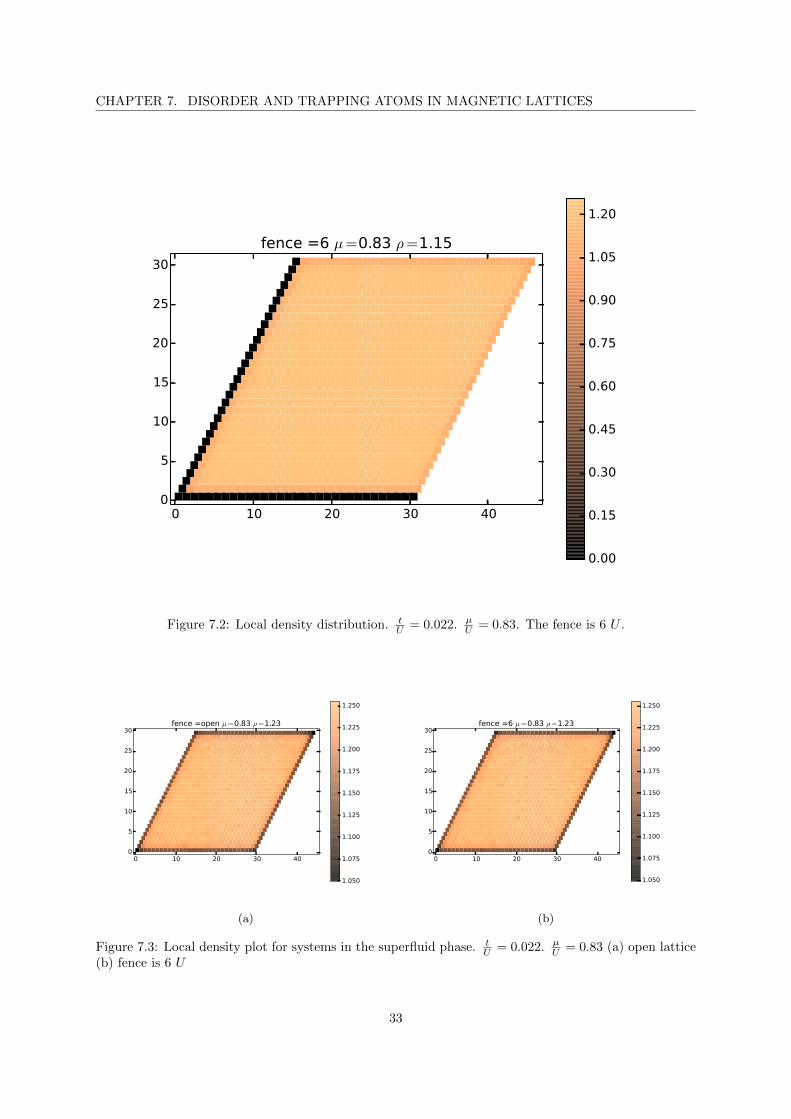
CHAPTER 7. DISORDER AND TRAPPING ATOMS IN MAGNETIC LATTICES
0 10 20 30 400
5
10
15
20
25
30
fence =6 µ=0.83 ρ=1.15
0.00
0.15
0.30
0.45
0.60
0.75
0.90
1.05
1.20
Figure 7.2: Local density distribution. tU = 0.022. µ
U = 0.83. The fence is 6 U .
0 10 20 30 400
5
10
15
20
25
30fence =open µ=0.83 ρ=1.23
1.050
1.075
1.100
1.125
1.150
1.175
1.200
1.225
1.250
(a)
0 10 20 30 400
5
10
15
20
25
30fence =6 µ=0.83 ρ=1.23
1.050
1.075
1.100
1.125
1.150
1.175
1.200
1.225
1.250
(b)
Figure 7.3: Local density plot for systems in the superfluid phase. tU = 0.022. µ
U = 0.83 (a) open lattice(b) fence is 6 U
33
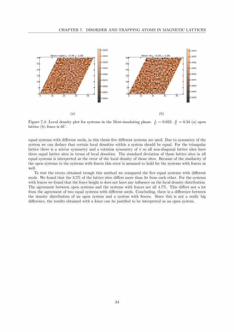
CHAPTER 7. DISORDER AND TRAPPING ATOMS IN MAGNETIC LATTICES
0 10 20 30 400
5
10
15
20
25
30fence =open µ=0.34 ρ=1.00
0.9930
0.9945
0.9960
0.9975
0.9990
1.0005
1.0020
1.0035
1.0050
(a)
0 10 20 30 400
5
10
15
20
25
30fence =6 µ=0.34 ρ=1.00
0.9930
0.9945
0.9960
0.9975
0.9990
1.0005
1.0020
1.0035
1.0050
(b)
Figure 7.4: Local density plot for systems in the Mott-insulating phase. tU = 0.022. µ
U = 0.34 (a) openlattice (b) fence is 6U .
equal systems with different seeds, in this thesis five different systems are used. Due to symmetry of thesystem we can deduce that certain local densities within a system should be equal. For the triangularlattice there is a mirror symmetry and a rotation symmetry of π so all non-diagonal lattice sites havethree equal lattice sites in terms of local densities. The standard deviation of those lattice sites in allequal systems is interpreted as the error of the local density of those sites. Because of the similarity ofthe open systems to the systems with fences this error is assumed to hold for the systems with fences aswell.
To test the errors obtained trough this method we compared the five equal systems with differentseeds. We found that the 3.5% of the lattice sites differs more than 3σ from each other. For the systemswith fences we found that the fence height is does not have any influence on the local density distribution.The agreement between open systems and the systems with fences are all 4.7%. This differs not a lotfrom the agreement of two equal systems with different seeds. Concluding, there is a difference betweenthe density distribution of an open system and a system with fences. Since this is not a really bigdifference, the results obtained with a fence can be justified to be interpreted as an open system.
34
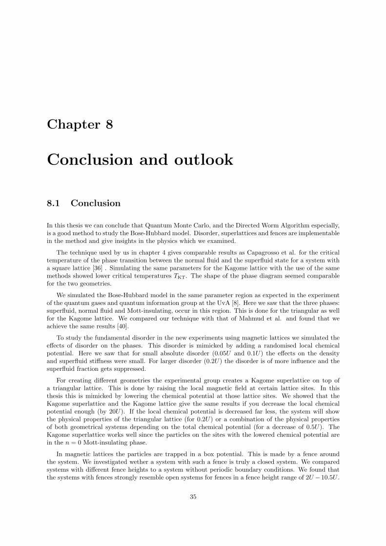
Chapter 8
Conclusion and outlook
8.1 Conclusion
In this thesis we can conclude that Quantum Monte Carlo, and the Directed Worm Algorithm especially,is a good method to study the Bose-Hubbard model. Disorder, superlattices and fences are implementablein the method and give insights in the physics which we examined.
The technique used by us in chapter 4 gives comparable results as Capagrosso et al. for the criticaltemperature of the phase transition between the normal fluid and the superfluid state for a system witha square lattice [36] . Simulating the same parameters for the Kagome lattice with the use of the samemethods showed lower critical temperatures TKT. The shape of the phase diagram seemed comparablefor the two geometries.
We simulated the Bose-Hubbard model in the same parameter region as expected in the experimentof the quantum gases and quantum information group at the UvA [8]. Here we saw that the three phases:superfluid, normal fluid and Mott-insulating, occur in this region. This is done for the triangular as wellfor the Kagome lattice. We compared our technique with that of Mahmud et al. and found that weachieve the same results [40].
To study the fundamental disorder in the new experiments using magnetic lattices we simulated theeffects of disorder on the phases. This disorder is mimicked by adding a randomised local chemicalpotential. Here we saw that for small absolute disorder (0.05U and 0.1U) the effects on the densityand superfluid stiffness were small. For larger disorder (0.2U) the disorder is of more influence and thesuperfluid fraction gets suppressed.
For creating different geometries the experimental group creates a Kagome superlattice on top ofa triangular lattice. This is done by raising the local magnetic field at certain lattice sites. In thisthesis this is mimicked by lowering the chemical potential at those lattice sites. We showed that theKagome superlattice and the Kagome lattice give the same results if you decrease the local chemicalpotential enough (by 20U). If the local chemical potential is decreased far less, the system will showthe physical properties of the triangular lattice (for 0.2U) or a combination of the physical propertiesof both geometrical systems depending on the total chemical potential (for a decrease of 0.5U). TheKagome superlattice works well since the particles on the sites with the lowered chemical potential arein the n = 0 Mott-insulating phase.
In magnetic lattices the particles are trapped in a box potential. This is made by a fence aroundthe system. We investigated wether a system with such a fence is truly a closed system. We comparedsystems with different fence heights to a system without periodic boundary conditions. We found thatthe systems with fences strongly resemble open systems for fences in a fence height range of 2U − 10.5U .
35
CHAPTER 8. CONCLUSION AND OUTLOOK
8.2 Outlook
More results can be obtained by having more CPU power. It is interesting to use this power to investigatethe extreme cases of U
t in the normal fluid to superfluid phase transition, where we can compare theanalytical results for the square lattice to that of the Kagome lattice. A higher precision in the results canbe obtained with more CPU power as well. This can be obtained by creating more points. Also, largersystem sizes will lead to smaller finite size effects and lower temperature to smaller finite temperatureeffects. For both more CPU power is necessary.
It is interesting to investigate further at which fence height the local density distribution starts todeviate more from the open lattice case.
36
Bibliography
[1] Richard P Feynman. Simulating physics with computers. International journal of theoretical physics,21(6/7):467–488, 1982.
[2] Dieter Jaksch, Ch Bruder, Juan Ignacio Cirac, Crispin W Gardiner, and Peter Zoller. Cold bosonicatoms in optical lattices. Physical Review Letters, 81(15):3108, 1998.
[3] Markus Greiner, Olaf Mandel, Tilman Esslinger, Theodor W Hansch, and Immanuel Bloch.Quantum phase transition from a superfluid to a mott insulator in a gas of ultracold atoms. nature,415(6867):39–44, 2002.
[4] V.Y.F. Leung, A. Tauschinsky, N.J. van Druten, and R.J.C. Spreeuw. Microtrap arrays on magneticfilm atom chips for quantum information science. Quantum Information Processing, 10(6):955–974,2011.
[5] I Herrera, Y Wang, P Michaux, D Nissen, P Surendran, S Juodkazis, S Whitlock, R J McLean,A Sidorov, M Albrecht, and P Hannaford. Sub-micron period lattice structures of magnetic micro-traps for ultracold atoms on an atom chip. Journal of Physics D: Applied Physics, 48(11):115002,2015.
[6] TG Tiecke, Jeffrey Douglas Thompson, Nathalie Pulmones de Leon, LR Liu, V Vuletic, andMikhail D Lukin. Nanophotonic quantum phase switch with a single atom. Nature, 508(7495):241–244, 2014.
[7] Fam Le Kien and A. Rauschenbeutel. Propagation of nanofiber-guided light through an array ofatoms. Phys. Rev. A, 90:063816, Dec 2014.
[8] Quantum Gases & Quantum Information group.http://iop.uva.nl/research/researchgroups/content/qgqi/quantum-gases-quantum-information.html.
[9] Lode Pollet. Ultracold atoms in an optical lattice: a numerical approach. Sort, 100:250, 2005.
[10] Alexander Altland and Ben D Simons. Condensed matter field theory. Cambridge University Press,2010.
[11] AJ Leggett. Superfluidity. Reviews of Modern Physics, 71:S318, 1999.
[12] Robert Roth and Keith Burnett. Phase diagram of bosonic atoms in two-color superlattices. PhysicalReview A, 68(2):023604, 2003.
[13] Matthew PA Fisher, Peter B Weichman, G Grinstein, and Daniel S Fisher. Boson localization andthe superfluid-insulator transition. Physical Review B, 40(1):546, 1989.
[14] Subir Sachdev. Quantum phase transitions. Wiley Online Library, 2007.
37
BIBLIOGRAPHY
[15] S Trotzky, L Pollet, F Gerbier, U Schnorrberger, Immanuel Bloch, NV Prokof’ev, Boris Svistunov,and M Troyer. Suppression of the critical temperature for superfluidity near the mott transition.Nature Physics, 6(12):998–1004, 2010.
[16] JM Kosterlitz and DJJ Thouless. Ordering metastability and phase transitions in two-dimensionalsystems. J. Phys. C, 6:1181, 1973.
[17] VL Berezinskii. Sov. Phys. JETP, 32:493, 1970.
[18] David R Nelson and JM Kosterlitz. Universal jump in the superfluid density of two-dimensionalsuperfluids. Physical Review Letters, 39(19):1201, 1977.
[19] Roger Eckhardt. Stan ulam, john von neumann, and the monte carlo method. Los Alamos Science,15:131–136, 1987.
[20] Nicholas Metropolis, Arianna W. Rosenbluth, Marshall N. Rosenbluth, Augusta H. Teller, andEdward Teller. Equation of state calculations by fast computing machines. The Journal of ChemicalPhysics, 21(6):1087–1092, 1953.
[21] Ulli Wolff. Collective monte carlo updating for spin systems. Physical Review Letters, 62(4):361,1989.
[22] Daniel Kandel and Eytan Domany. General cluster monte carlo dynamics. Physical Review B,43(10):8539, 1991.
[23] CM Fortuin. Physica (utrecht) 57, 536 (1972); pw kasteleyn and cm fortuin. J. Phys. Soc. Jpn.Suppl, 26(11), 1969.
[24] P.R. Corboz. Advanced numerical methods in many-body physics, 2015.
[25] Robert H Swendsen and Jian-Sheng Wang. Nonuniversal critical dynamics in monte carlo simula-tions. Physical review letters, 58(2):86, 1987.
[26] B Bauer, L D Carr, H G Evertz, A Feiguin, J Freire, S Fuchs, L Gamper, J Gukelberger, E Gull,S Guertler, A Hehn, R Igarashi, S V Isakov, D Koop, P N Ma, P Mates, H Matsuo, O Parcollet,G Pawowski, J D Picon, L Pollet, E Santos, V W Scarola, U Schollwck, C Silva, B Surer, S Todo,S Trebst, M Troyer, M L Wall, P Werner, and S Wessel. The alps project release 2.0: open sourcesoftware for strongly correlated systems. Journal of Statistical Mechanics: Theory and Experiment,2011(05):P05001, 2011.
[27] Ping Nang Ma. Numerical simulations of bosons and fermions in three dimensional optical lattices.PhD thesis, ETH Zurich, 2013.
[28] Hans Gerd Evertz, Gideon Lana, and Mihai Marcu. Cluster algorithm for vertex models. Physicalreview letters, 70(7):875, 1993.
[29] Olav F Syljuasen and Anders W Sandvik. Quantum monte carlo with directed loops. PhysicalReview E, 66(4):046701, 2002.
[30] NV Prokof?ev, BV Svistunov, and IS Tupitsyn. Exact, complete, and universal continuous-timeworldline monte carlo approach to the statistics of discrete quantum systems. Journal of Experi-mental and Theoretical Physics, 87(2):310–321, 1998.
[31] Lode Pollet, Kris Van Houcke, and Stefan MA Rombouts. Engineering local optimality in quantummonte carlo algorithms. Journal of Computational Physics, 225(2):2249–2266, 2007.
[32] Prokof’ev N Svistunov B. Understanding Quantum Phase Transitions, chapter Worm Algorithm forProblems of Quantum and Classical Statistics. Taylor and Francis, 2009.
38
BIBLIOGRAPHY
[33] Guido Schmid, Synge Todo, Matthias Troyer, and Ansgar Dorneich. Finite-temperature phasediagram of hard-core bosons in two dimensions. Phys. Rev. Lett., 88:167208, Apr 2002.
[34] Kenji Harada and Naoki Kawashima. Universal jump in the helicity modulus of the two-dimensionalquantum xy model. Phys. Rev. B, 55:R11949–R11952, May 1997.
[35] Boris V Svistunov, Egor S Babaev, and Nikolay V Prokof’ev. Superfluid states of matter. Crc Press,2015.
[36] Barbara Capogrosso-Sansone, Sebnem Gune s Soyler, Nikolay Prokof’ev, and Boris Svistunov.Monte carlo study of the two-dimensional bose-hubbard model. Phys. Rev. A, 77:015602, Jan2008.
[37] Juan Carrasquilla and Marcos Rigol. Superfluid to normal phase transition in strongly correlatedbosons in two and three dimensions. Physical Review A, 86(4):043629, 2012.
[38] Nikolay Prokof’ev, Oliver Ruebenacker, and Boris Svistunov. Critical point of a weakly interactingtwo-dimensional bose gas. Physical review letters, 87(27):270402, 2001.
[39] Fabrice Gerbier, Artur Widera, Simon Folling, Olaf Mandel, Tatjana Gericke, and Immanuel Bloch.Interference pattern and visibility of a mott insulator. Physical Review A, 72(5):053606, 2005.
[40] K. W. Mahmud, E. N. Duchon, Y. Kato, N. Kawashima, R. T. Scalettar, and N. Trivedi. Finite-temperature study of bosons in a two-dimensional optical lattice. Phys. Rev. B, 84:054302, Aug2011.
[41] F. A. Tauschinsky. Rydberg Atoms on a Chip and in a Cell. PhD thesis, University of Amsterdam,2013.
[42] Julia Stasinska, Mateusz Lacki, Omjyoti Dutta, Jakub Zakrzewski, and Maciej Lewenstein. Bose-hubbard model with random impurities: Multiband and nonlinear hopping effects. Phys. Rev. A,90:063634, Dec 2014.
39
Recommended