UNIVERSITA DEGLI STUDI DI PARMA
Dottorato di Ricerca in Matematica Pura e Applicata
Ciclo XXVII
High order semi-Lagrangian methods
for BGK-type models in the kinetic theory
of rarefied gases
Coordinatore:
Chiar.ma Prof.ssa Alessandra Lunardi
Tutor:
Chiar.ma Prof.ssa Maria Groppi
Co-Tutor:
Chiar.mo Prof. Giovanni Russo
Dottorando: Giuseppe Stracquadanio
GENNAIO 2015

Contents
Introduction 7
1 The Boltzmann equation and the BGK model 11
1.1 Boltzmann equation . . . . . . . . . . . . . . . . . . . . . . . . . . . . . . . 12
1.2 Physical properties . . . . . . . . . . . . . . . . . . . . . . . . . . . . . . . . 13
1.2.1 Macroscopic moments . . . . . . . . . . . . . . . . . . . . . . . . . . 13
1.2.2 Collision invariants and Maxwellian equilibria . . . . . . . . . . . . . 14
1.2.3 H-theorem. . . . . . . . . . . . . . . . . . . . . . . . . . . . . . . . . 16
1.2.4 Entropy inequality . . . . . . . . . . . . . . . . . . . . . . . . . . . . 17
1.2.5 Fluid limit . . . . . . . . . . . . . . . . . . . . . . . . . . . . . . . . 18
1.3 BGK model . . . . . . . . . . . . . . . . . . . . . . . . . . . . . . . . . . . . 19
1.4 Chu reduction . . . . . . . . . . . . . . . . . . . . . . . . . . . . . . . . . . . 22
2 Basic numerical methods for evolutionary PDEs 25
2.1 Runge-Kutta methods for ODEs . . . . . . . . . . . . . . . . . . . . . . . . 25
2.1.1 One-step methods for ODEs . . . . . . . . . . . . . . . . . . . . . . . 26
2.1.2 Runge-Kutta methods . . . . . . . . . . . . . . . . . . . . . . . . . . 27
2.1.3 Stability analysis for Runge-Kutta methods . . . . . . . . . . . . . . 28
2.1.4 L-stability . . . . . . . . . . . . . . . . . . . . . . . . . . . . . . . . . 30
2.2 Multi-step methods . . . . . . . . . . . . . . . . . . . . . . . . . . . . . . . . 31
2.2.1 Adams methods . . . . . . . . . . . . . . . . . . . . . . . . . . . . . 31
2.2.2 BDF methods . . . . . . . . . . . . . . . . . . . . . . . . . . . . . . . 32
2.2.3 Local error and order conditions . . . . . . . . . . . . . . . . . . . . 32
2.2.4 Stability and the first Dahlquist barrier . . . . . . . . . . . . . . . . 33
2.2.5 A-Stability for multi-step methods . . . . . . . . . . . . . . . . . . . 34
2.3 High order non oscillatory reconstruction . . . . . . . . . . . . . . . . . . . 35
2.3.1 The ENO approximation . . . . . . . . . . . . . . . . . . . . . . . . 36
2.3.2 The WENO approximation . . . . . . . . . . . . . . . . . . . . . . . 38
3
Contents 4
2.3.3 General WENO reconstruction . . . . . . . . . . . . . . . . . . . . . 39
2.3.4 Second-third order WENO interpolation . . . . . . . . . . . . . . . . 40
2.3.5 Third-fifth order WENO interpolation . . . . . . . . . . . . . . . . . 40
2.4 Semi-Lagrangian schemes . . . . . . . . . . . . . . . . . . . . . . . . . . . . 41
2.4.1 Simple semi-Lagrangian examples of approximation schemes . . . . . 42
2.4.2 CFL condition for semi-Lagrangian schemes . . . . . . . . . . . . . . 44
3 Semi-Lagrangian schemes applied to BGK equation 47
3.1 Lagrangian formulation and first order scheme . . . . . . . . . . . . . . . . 47
3.2 High order Runge-Kutta methods . . . . . . . . . . . . . . . . . . . . . . . . 50
3.2.1 Second order Runge-Kutta method . . . . . . . . . . . . . . . . . . . 51
3.2.2 Third order Runge-Kutta method . . . . . . . . . . . . . . . . . . . 52
3.3 BDF methods . . . . . . . . . . . . . . . . . . . . . . . . . . . . . . . . . . . 53
3.3.1 Second order BDF method. . . . . . . . . . . . . . . . . . . . . . . . 54
3.3.2 Third order BDF method. . . . . . . . . . . . . . . . . . . . . . . . . 55
3.4 Semi-lagrangian schemes without interpolation . . . . . . . . . . . . . . . . 58
3.4.1 Construction of suitable high order Runge-Kutta schemes which
avoid interpolation . . . . . . . . . . . . . . . . . . . . . . . . . . . . 58
3.5 Chu reduction model . . . . . . . . . . . . . . . . . . . . . . . . . . . . . . . 60
3.6 Numerical tests . . . . . . . . . . . . . . . . . . . . . . . . . . . . . . . . . . 62
3.6.1 Test 1: regular velocity perturbation . . . . . . . . . . . . . . . . . . 63
3.6.2 Optimal CFL . . . . . . . . . . . . . . . . . . . . . . . . . . . . . . . 66
3.6.3 Test 2: Riemann problem . . . . . . . . . . . . . . . . . . . . . . . . 69
3.6.4 Semi-Lagrangian schemes without interpolation . . . . . . . . . . . . 72
3.6.5 Numerical results - Chu reduction . . . . . . . . . . . . . . . . . . . 74
3.7 Hybrid order schemes . . . . . . . . . . . . . . . . . . . . . . . . . . . . . . 76
4 Gas-surface interaction and boundary conditions 83
4.1 Numerical treatment of the boundary conditions . . . . . . . . . . . . . . . 85
4.1.1 Specular reflection . . . . . . . . . . . . . . . . . . . . . . . . . . . . 85
4.1.2 Diffusive condition . . . . . . . . . . . . . . . . . . . . . . . . . . . . 86
4.2 Inverse Lax-Wendroff technique . . . . . . . . . . . . . . . . . . . . . . . . . 90
4.3 Numerical test . . . . . . . . . . . . . . . . . . . . . . . . . . . . . . . . . . 90
4.3.1 Smooth solutions . . . . . . . . . . . . . . . . . . . . . . . . . . . . . 91
4.3.2 Flow generated by a gradient of temperature. . . . . . . . . . . . . . 92
4.4 WENO type extrapolation . . . . . . . . . . . . . . . . . . . . . . . . . . . . 93
5 Contents
5 BGK models for gas mixtures and semi-Lagrangian approximation 97
5.1 Boltzmann equation for inert gas mixtures . . . . . . . . . . . . . . . . . . . 97
5.2 BGK models for inert gas mixtures . . . . . . . . . . . . . . . . . . . . . . . 100
5.2.1 The BGK model of Andries, Aoki and Perthame . . . . . . . . . . . 100
5.2.2 A new BGK model for inert mixtures . . . . . . . . . . . . . . . . . 102
5.3 BGK model for reactive mixtures . . . . . . . . . . . . . . . . . . . . . . . . 106
5.3.1 The BGK model of Groppi and Spiga . . . . . . . . . . . . . . . . . 107
5.4 Numerical treatment . . . . . . . . . . . . . . . . . . . . . . . . . . . . . . . 108
5.4.1 First order SL scheme for the AAP BGK model . . . . . . . . . . . 108
5.4.2 Sketch of the first order SL scheme for the reactive BGK model . . . 112
5.5 Numerical results . . . . . . . . . . . . . . . . . . . . . . . . . . . . . . . . . 113
Conclusions and Perspectives 125

Contents 6
Introduction
In hydrodynamic regimes, fluid flows can be described by standard models such as Navier-
Stokes or compressible Euler equations. However, some regimes cannot be qualified as hy-
drodynamic and the continuum equations are not able to correctly describe the dynamics
of the flow. The parameter that dictates whether or not a flow is hydrodynamic is the
Knudsen number Kn. It is defined as the ratio between the mean free path λ between the
particles and the characteristic length of the physical problem L. When this number goes
to zero, the hydrodynamic regime is reached. For large Knudsen number (usually higher
than 10−2), the regime is qualified as rarefied and it is well described by the kinetic theory
and in particular by the Boltzmann equation, an integro-differential equation governing
the evolution of the so called distribution function in the phase space [13].
Traditionally, an important field of application of kinetic theory has been the motion of
objects in the rarefied layers of the atmosphere, such as re-entry problems in aerospace
engineering. Indeed, in these cases, the Knudsen number is large, because the mean free
path is of orders of magnitude larger than the characteristic length of the space vehicle.
Recently, however, a huge new field of applications of kinetic theory has begun to develop
in the modeling of fluid flows in nanotechnology, for example to build Micro-Electro-
Mechanical-Systems (MEMS) [14], which are present in accelerometers, micro pumps or
micro engines: in this case, the Knudsen number is large because the scale of interest L is
so small that the ratio λ/L is of order one and microscopic effects cannot be neglected.
Approximate methods of solution for the Boltzmann equation have a long history tracing
back to Hilbert, Chapman and Enskog [13] at the beginning of the last century. The
mathematical difficulties related to the Boltzmann equation make it extremely difficult to
treat; in particular, analytical solutions in most relevant situations are hard (and some-
times impossible) to find. Most of the difficulties are due to the multidimensional structure
of the collision integral. In addition, the numerical integration requires great care since
the collision integral is at the basis of the macroscopic properties of the equation. Further
7
Introduction 8
difficulties rely on the presence of stiffness, like in the case of small mean free path or of
large velocities.
For such reasons many realistic numerical simulations are based on Monte-Carlo tech-
niques. The most famous examples are Direct Simulation Monte Carlo [6], which is a
particle solver especially efficient in the rarefied regime. However, the computational time
requirement increases very rapidly as the hydrodynamic regime is reached. The number
of collisions increases and a strong restriction appears on the time step. For this reason,
attempts have been made to derive numerical solvers for the Boltzmann equation which
are not based on particles.
Among deterministic approximation, one of the most popular methods is represented by
the so called Discrete Velocity Models (DVM) of the Boltzmann equation [10, 46]. These
methods are based on a Cartesian grid in velocity and on a discrete collision mechanism
on the points of the grid that preserves the main physical properties. Unfortunately DVM
are not competitive with Monte Carlo methods in terms of computational cost.
A reduction of computation time is possible by considering simplified models of the Boltz-
mann equation. A particularly successful model is the BGK model [8], in which the col-
lision term of the Boltzmann equation is replaced by a relaxation term, simpler to treat.
The BGK model by construction reproduces several physical properties of the Boltzmann
equation and is consistent with the hydrodynamic limit at the continuous level, i.e., for
very small Knudsen numbers the Euler limit is recovered. The numerical schemes used to
solve the BGK model that fulfill this property are called asymptotic preserving (AP), after
the pioneering work by Jin [31]. For small relaxation time, a strong restriction on the time
step exists also for the BGK model, but it can be easily treated by using implicit schemes.
Among these implicit schemes, we have to mention Implicit-Explicit Runge-Kutta meth-
ods (IMEX)[40, 42]. We focus here our attention on implicit semi-Lagrangian schemes for
the BGK equation [49, 50, 51].
This thesis presents high order shock capturing semi-Lagrangian methods for the nu-
merical solutions of BGK-type equations. The starting point is the work of Santagati
and Russo [49, 51]. They have developed implicit semi-Lagrangian schemes for the one-
dimensional BGK model. The key idea of the semi-Lagrangian formulation is to integrate
partial differential equations along the characteristics and then its main advantage is that
PDEs become ODEs along such curves. Moreover, semi-Lagrangian schemes allow us to
use large time steps, avoiding the classical Courant stability condition. Contrary, the
main drawback is that some interpolation is required in order to reconstruct the solution
on the feet of the characteristics. The need for a spatial reconstruction could become a
9
drawback when we are looking for high order methods. Indeed, the computational cost
can increase considerably. In detail, in [49, 51] these problems are dealt with L-stable
diagonally implicit Runge-Kutta (DIRK) coupled with a WENO-type spatial reconstruc-
tion. The choice of DIRK methods allows to avoid strong restrictions on the time step,
and the use of a WENO reconstruction allows to preserve accuracy also in stiff regime and
in presence of discontinuities.
In the present thesis some substantial improvements of these semi-Lagrangian schemes
for the BGK equation are proposed, together with some new applications.
First of all, we tried to reduce the computational cost, due mainly to the interpolation
technique. We investigated two directions [24]: the use of multi-step methods instead of
DIRK methods and the development of particular semi-Lagrangian schemes that avoid
completely spatial interpolation. In the development of high order methods, we observed
that the number of spatial interpolations required at each step increases as the order of
the method. In particular a DIRK method required 1, 3 or 6 interpolations at each time
step to obtain respectively a first, second or third order method. Instead, using multi-step
methods, such as backward differentiation formula (BDF) methods, the number of inter-
polations is 1, 2 and 3, respectively. Thus the use of BDF methods reduces considerably
the computational cost, in particular for high order.
The study of methods that avoid interpolation also deserves attention [24]. Interpola-
tion techniques in semi-Lagrangian schemes are required because in general the feet of
the characteristic lines are not grid points. Thus if we want to avoid interpolation, we
have to find a trick in such a way the feet of characteristics coincide with the grid points.
This can be obtained imposing some restriction on the choice of the time step. Numerical
experiments show that schemes without interpolation can be cost-effective, especially for
problems that do not require a fine mesh in velocity.
Then we investigated some applications and extensions to more physical interesting prob-
lems of the numerical schemes proposed for the one dimensional BGK equation. By means
of the Chu reduction [15], we extended the schemes to more realistic physical domains,
3D in velocity. Moreover, we considered boundary-value problems and we studied the
treatment of reflective and diffusive boundary conditions. Finally, the methods have been
extended to different BGK models for inert and reactive gas mixtures.
The thesis is organized as follows. We start by recalling the Boltzmann equation, its main
physical properties and the BGK model in Chapter 1. In Chapter 2 we introduce the
basics of the Runge-Kutta methods , multi-step methods, WENO reconstruction. Next in

Introduction 10
Chapter 3, we present the high order semi-Lagrangian schemes for the BGK equation and
their properties. The extension of the methods to treat boundary conditions is presented
in Chapter 4. Finally, applications of the numerical schemes to BGK-type equations for
gas mixtures both inert and reactive, are described in Chapter 5.
Chapter 1
The Boltzmann equation and the
BGK model
Historically, kinetic theory arises for the mathematical modeling of rarefied gas dynamics.
What is a rarefied gas?
A gas can be thought as a collection of a huge number of molecules moving freely in
space, tending to occupy all the available volume. In the trajectory of a molecule one can
distinguish two phases: a phase of free motion, in which the molecule is not affected by
the presence of other molecules, and a phase of collision, strongly localized in space and
time, in which the molecule collides with another molecule, significantly deviating from
the path that would be followed in free flight. The size of the region of space in which
the collision takes place is of the order of magnitude of the radius of action of the internal
forces, which in turn is of the order of the molecular dimensions. Denote by d this typical
size and by λ the mean free path of the molecules, that is the average distance between
two subsequent collisions. When
d
λ<< 1,
the molecule is spending most of its time in the phase of free flight with collision practically
localized and instantaneous, we are in presence of a rarefied gas.
Kinetic theory represents a mesoscopic approach which lies between the macroscopic and
the microscopic one, looking at both aspects. Kinetic theory takes into account collisions
between particles, but describes their motion without following the individual trajectories
and using instead probabilistic considerations and methods of statistical mechanics, which
quantify the collective effects in an appropriate balance equation, the Boltzmann equation.
11
Chapter 1. The Boltzmann equation and the BGK model 12
1.1 Boltzmann equation
The Boltzmann equation is named after the Austrian physicist and mathematician Ludwig
Boltzmann, who proposed it in 1872 for the first time [13]. The unknown is the distribution
function f(t, x, v), defined in the phase space, (t, x, v) ∈ R+ × RD × RN where D and N
denote the dimension of the physical and velocity spaces respectively. The Boltzmann
equation reads as∂f
∂t+ v · ∇xf = Q(f, f) (1.1)
with initial data
f(t, x, v) = f0(x, v),
and describes the time evolution of a monoatomic rarefied gas of particles which move
with velocity v ∈ RN in the position x ∈ RD at time t > 0. The term v · ∇xf is the
so-called streaming term, which describes the free flight of the particles.
The bilinear collision (integral) operator Q(f, f), which describes the binary collisions of
the particles, acts over the velocity variable only
Q(f, f)(v) =
∫
RN
∫
S2B(v, w,Ω)[f(v′)f(w′)− f(v)f(w)] dΩ dw. (1.2)
In the above expression, Ω is a unit vector of the sphere S2 and (v′, w′) represents the post-
collisional velocities associated with the pre-collisional velocities (v, w). The collisional
velocities satisfy microscopic momentum and energy conservations
v′ + w′ = v + w, |v′|2 + |w′|2 = |v|2 + |w|2. (1.3)
Moreover, each collision satisfies of course microscopic mass conservation. The above
system of algebraic equations has the following parametrized solution
v′ =1
2(v + w + |v − w|Ω), w′ =
1
2(v + w − |v − w|Ω), (1.4)
where |v − w| is the relative speed and Ω is the unit vector of the post-collision relative
velocity v′ − w′ = g′.
The collision kernel B(v, w,Ω) is a non negative function which characterizes the details of
the binary interactions and depends only on |v−w| and on the scattering angle χ between
pre- and post collision relative velocities v − w and v′ − w′ = |v − w|Ω, with
cosχ =(v − w) · Ω|v − w| .
The collision kernel has the form
B(v, w,Ω) = |v − w|σ(|v − w|, cosχ),
13 1.2. Physical properties
where the function σ is the scattering cross-section. In the case of inverse k − th power
forces between particles, the collision kernel has the form
σ(|v − w|, cosχ) = bα(cosχ)|v − w|α−1, B(v, w,Ω) = bα(cosχ)|v − w|α,
with α = (k − 5)/(k − 1). For k > 5 we have hard potentials, for k < 5 we have soft
potentials. The special situation k = 5 gives the Maxwellian model with
B(v, w,Ω) = b0(cosχ).
1.2 Physical properties
1.2.1 Macroscopic moments
The Boltzmann equation, thanks to the mesoscopic nature of the kinetic approach, takes
into account the microscopic collisions between the particles, giving us macroscopic in-
formation about the time evolution of the process involving the gas. Indeed, once the
distribution function f is known, one is able to recover the macroscopic fields such as
macroscopic density ρ(t, x), macroscopic velocity u(t, x) and macroscopic temperature
T (t, x).
The distribution function, from a physical point of view, tells us how the molecules of the
gas are distributed in the phase space. Therefore, to obtain the numerical density n(t, x)
in the physical space, since f(t, x, v) is the number of molecules in x at time t and with
velocity v, the total number of molecules in x at time t is given by
n(t, x) =
∫
RNf(t, x, v) dv.
Then the mass density, or macroscopic density, is given by ρ(t, x) = mn(t, x), where m is
the particle mass. This gives us another key interpretation about the distribution function.
Indeed ∫
RN
1
n(t, x)f(t, x, v) dv = 1,
so f/n can be seen as a probability density with respect to the kinetic variable v, that is,1
nf dv is the probability to find out a particle in dv, at time t, in the position x.
Now, following the same argument, the mean velocity of the gas is given by
u(t, x) =1
n(t, x)
∫
RNv f(t, x, v) dv.
Therefore, the momentum density is
ρu =
∫
RNmv f(t, x, v) dv.
Chapter 1. The Boltzmann equation and the BGK model 14
The kinetic energy density is
E(t, x) =
∫
RN
1
2mv2 f(t, x, v) dv.
The kinetic energy E(t, x) is related to the temperature T (t, x) by the underlying relation
E =1
2ρu2 +
N
2ρRT,
where R is the gas constant, that is related to the Boltzmann constant KB by the expres-
sion KB = mR.
Resuming, the first macroscopic fields (density, momentum, kinetic energy) can be com-
puted in this way:
(ρ, ρu,E)T = 〈fφ(v)〉, where φ(v) =(m,mv,
1
2mv2
)T, 〈g〉 =
∫
RNg(v) dv. (1.5)
1.2.2 Collision invariants and Maxwellian equilibria
The macroscopic moments considered in (1.5) are relevant to molecular properties which
are conserved by collisions, the so called collision invariants. Hereafter, we assume that
f ∈ B, where B denotes the space of admissible functions for the distribution function f.
Essential properties of the elements of B are positivity and integrability. From one case
to another, smooth properties will be specified.
We consider a class of function φ(v), smooth respect to v, and we compute the weak
form of collision operator Q(f, f)∫
RNQ(f, f)φ(v) dv. (1.6)
We observe that, if φ(v) is a molecular property, (1.6) represents the production of this
molecular property due to collisions. For any test function φ(v) it can be proved [13] that∫
RNQ(f, f)φ(v) dv =
− 1
4
∫
RN×RN×S2B(v, w,Ω)[f(v′)f(w′)− f(v)f(w)][φ(v′) + φ(w′)− φ(v)− φ(w)] dΩ dw dv
(1.7)
where we have omitted the explicit dependence from t and x for the sake of simplicity.
In particular, we can choose 1, v, and v2 as test function. Due to the microscopic mass,
momentum and energy conservation (1.3) one can obtain easily that∫
RNQ(f, f) dv = 0,
15 1.2. Physical properties
∫
RNQ(f, f) v dv = 0,
∫
RNQ(f, f) v2 dv = 0, (1.8)
in others words, there is no production of mass, momentum and energy due to colli-
sions. The molecular properties which do not vary through collisions are called collision
invariants, according to the following definition
Definition 1.1. Each test function φ(v) which satisfies
φ(v) + φ(w) = φ(v′) + φ(w′) ∀(v, w,Ω) ∈ RN × RN × S2 (1.9)
is called collision invariant.
The following results can be proved [13]
Theorem 1.2.1. Let φ ∈ C0 be a collision invariant. Then there exist unique a, c ∈ R,and b ∈ RN such that
φ(v) = a+ b · v + cv2. (1.10)
Lemma 1.2.2 (Boltzmann’s lemma). Let W [f ] be the function
W [f ] =
∫
RNln fQ(f, f) dv. (1.11)
Then W [f ] satisfies the following two properties:
- W [f ] ≤ 0 ∀f ∈ B,
- W [f ] = 0⇔ f(v′)f(w′) = f(v)f(w) ∀(v, w,Ω) ∈ RN × RN × S2,
where v′ and w′ are given by (1.4.)
Proof. By (1.7) for φ(v) = ln f we have
−W [f ] =
=1
4
∫
RN×RN×S2B(v, w,Ω)[f(v′)f(w′)−f(v)f(w)][ln(f(v′)f(w′))− ln(f(v)f(w))] dΩ dw dv
=1
4
∫
RN×RN×S2B(v, w,Ω) ln
(f(v′)f(w′)f(v)f(w)
)(f(v′)f(w′)f(v)f(w)
− 1
)f(v)f(w) dΩ dw dv,
where B(v, w,Ω) and f are positive. Because the function g(x) = (x− 1) lnx with x ≥ 0
satisfies
- g(x) ≥ 0 ∀x > 0,
Chapter 1. The Boltzmann equation and the BGK model 16
- g(x) = 0⇔ x = 1,
the thesis is proved.
Definition 1.2. The distribution functions f ∈ B such that
Q(f, f)(v) = 0, ∀v ∈ RN
are said equilibrium distributions.
Through Boltzmann’s lemma 1.2.2 it is possible to state the following equivalence:
f is a collision equilibrium⇔ ln(f) is a collision invariant.
Thanks to Theorem 1.2.1 we get:
f is a collision equilibrium⇔ ∃ a, c ∈ R, and b ∈ RN such that ln f(v) = a+ b · v + cv2
⇔ ∃ a, c ∈ R, and b ∈ RN such that f(v) = ea+b·v+cv2 .
The last expression characterizes all the possible collision equilibria. Since f must be
integrable, c must be strictly negative. Computing the macroscopic fields of the collision
equilibria, we get
f(t, x, v) = M(ρ, u, T )(t, x, v) =ρ(t, x)
(2πRT (t, x))N/2exp
(− |v − u(t, x)|2
2RT (t, x)
), (1.12)
where ρ, u and T are the macroscopic density, velocity and temperature. The functions
(1.12) are the so-called Maxwellian distributions. If (1.12) does not depend on x and t we
have an absolute Maxwellian, otherwise a local Maxwellian. The H-theorem, given in the
next section, will focus on the trend to equilibrium of the distribution function, solution
of the Boltzmann equation.
1.2.3 H-theorem.
In this paragraph we investigate the effects of the collisions on the time evolution of
the distribution function. The H-theorem is one of the most important results in this
framework. It is based on the introduction of a function, the H function, which is directly
related to the irreversibility of the physical process and to the entropy of the system. We
focus on the effects of the collisions and then we consider the Boltzmann equation in a
spatially uniform state (∇xf = 0) with no external forces
∂f
∂t= Q(f, f). (1.13)
17 1.2. Physical properties
Let H[f ] : B→ R be the H-function defined as follow,
H[f ] =
∫
RNf(t, v) ln(f(t, v)) dv. (1.14)
Definition (1.14) shows that the H function depends only on time t. The time derivative
leads to
d
dtH[f ](t) =
d
dt
∫
RNf(t, v) ln(f(t, v)) dv =
∫
RN
(∂f
∂tln f + f
1
f
∂f
∂t
)dv
=
∫
RNln fQ(f, f) dv +
d
dt
∫
RNf dv = W [f ]. (1.15)
Therefore, thanks to the Boltzmann’s lemma 1.2.2, the Boltzmann H-theorem states that
∂H
∂t≤ 0, (1.16)
and the equality holds only if and only if f is a collision equilibrium, that is, a local
Maxwellian.
Boltzmann’s H-theorem implies that the H function is a Lyapunov function for the local
Maxwellian.This stresses the importance of the Maxwellian distribution functions, because
each state evolves in time towards them.
1.2.4 Entropy inequality
Instead of considering (1.13), if we take into account the complete Boltzmann equation
(1.1), we obtain the entropy inequality by the same steps of the previous paragraph.
Let φ(v) = −R ln(f) = −KBm ln(f) be a test function. We define the entropy s as
s =
∫
RNf(v)φ(v) dv = −KB
ρ
∫
RNf ln f dv = −KB
ρH, (1.17)
where H is the H-function. Now, we define the entropy flux h and the entropy production
Σ
h = −KB
m
∫
RNvf ln(f) dv,
Σ = −KB
m
∫
RNln(f)Q(f, f) dv = −KB
mW [f ] ≥ 0.
The weak form of (1.1) with φ(v) = −KBm ln(f) is
∂
∂t(ns) +∇ · h = Σ.
Due to the Boltzmann’s lemma and the entropy production expression, the last equation
becomes∂
∂t(n s) +∇ · h ≥ 0 (1.18)
that is the entropy inequality.
Chapter 1. The Boltzmann equation and the BGK model 18
1.2.5 Fluid limit
By (1.8), if we multiply the Boltzmann equation by the collision invariants φ(v) = m, mv,12mv
2 and integrate on velocity space we obtain
∂
∂t
∫
RNfφ(v) dv +∇x
(∫
RNvfφ(v) dv
)= 0. (1.19)
These equations describe the balance of mass, momentum and energy. The system of five
equations is not closed since it involves higher order moments of the distribution function
f , in addition to ρ, u, and T.
Let L be a characteristic length of the problem, and λ the mean free path. From the
comparison between λ and L we can deduce important information about the behavior of
the gas. Let us define
Kn =λ
L.
The parameter Kn is called the Knudsen number. If Kn ∼ O(1), that is L ∼ λ, the
particles cover a relative long distance between two subsequent collisions and the evolution
is governed mainly by the free flow, namely by the streaming operator in the Boltzmann
equation. In this case we state that we are in a rarefied regime. On the contrary, if
Kn → 0, that is λ << L, the particles will undergo a great number of collisions on a
macroscopic significant distance. This is the regime where the evolution is governed by
collisions and it is called hydrodynamic or fluid regime. In order to point out the different
scaling between the physical quantities in different regimes, it could be useful to consider
the dimensionless scaled Boltzmann equation
∂f
∂t+ v · ∇xf =
1
KnQ(f, f) (1.20)
where, for simplicity, we denote by the same symbols the physical dimensionless quantity
used.
As Kn → 0, the collisions become more and more important and (1.20) formally be-
comes Q(f, f) → 0, and thus f approaches the local Maxwellian. In this case the higher
order moments of the distribution function can be computed as function of ρ, u, and T
and by (1.19) we obtain the closed system of compressible Euler equations
∂ρ
∂t+∇x · (ρu) = 0
∂ρu
∂t+∇x · (ρu⊗ u+ pI) = 0
19 1.3. BGK model
∂E
∂t+∇x · (Eu+ pu) = 0
p = ρT, E =N
2ρRT +
1
2ρu2
where p is the gas pressure and ⊗ denotes the tensor product.
The rigorous passage from the Boltzmann equation to the compressible Euler equations has
been investigated by several authors. Among them we mention [12, 38]. Higher order fluid
models, such as the Navier-Stokes model, can be obtained from the Boltzmann equation
using the Chapman-Enskog and the Hilbert expansions.
1.3 BGK model
One of the main shortcomings in dealing with the Boltzmann equation is the complicated
structure of the collision integral (1.2).
It is therefore not surprising that alternative, simpler expressions have been proposed for
the collision term; they are known as collision models, and any Boltzmann-like equation
where the Boltzmann collision integral is replaced by a collision model is called a model
equation or a kinetic model [13].
The idea behind this replacement is that a large amount of detail of the collisions (which
are contained in the collision term) is not likely to influence significantly the values of
many experimentally measured quantities. That is, unless very refined experiments are
devised, it is expected that the fine structure of the collision operator can be replaced by
a blurred image, based upon a simpler operator which retains only the qualitative and
average properties of the true collision operator.
The most widely known collision model is usually called the Bhatnagar, Gross and Krook
(BGK, 1954) model [8], although Welander proposed it independently [58]. The idea
behind the BGK model is that the essential features of a collision operator are:
the true collision term satisfies Eq. (1.8). Hence the BGK collision term must also
satisfy them;
moreover, the BGK model must satisfy the Boltzmann H-theorem (1.16), with equal-
ity holding if, and only if, f is a Maxwellian.
As we have seen in section 1.2.2, this second property expresses the tendency of the gas to
a Maxwellian distribution. The simplest way of taking this feature into account seems to
assume that the average effect of collisions is to change the distribution function f by an
amount proportional to the departure of f from a Maxwellian M [f ]. So, if ε is a constant
Chapter 1. The Boltzmann equation and the BGK model 20
with respect to v, the BGK model reads as the following initial value problem
∂f
∂t+ v · ∇xf = QBGK [f ] ≡ 1
ε(M− f), (t, x, v) ∈ R+ × RD × RN
f(0, x, v) = f0(x, v),
(1.21)
where D and N denote the dimension of the physical and velocity spaces respectively,
and ε is the relaxation time, that is of the order of the Knudsen number; M denotes a
local Maxwellian. Therefore it has the same form of (1.12), but it depends on auxiliary
parameters ρ, u and T . His expression is:
M =ρ
[2πRT
]N/2 exp
(− (v − u)2
2RT
). (1.22)
The free parameters ρ, u and T , are introduced in such a way that the BGK relaxation
operator satisfies the main properties of the collision operator Q(f, f). First of all, the
collision operator of the Boltzmann equation satisfies (1.8), therefore, also for the relax-
ation operator QBGK [f ], the functions 1, v and v2 must be collision invariants. In this
way, the new operator does not have production of mass, momentum and energy. Thus,
it is needed that the weak form of QBGK [f ] vanishes for φ(v) = 1, v and v2, that is∫
RN(1, v, v2)M(v) dv =
∫
RN(1, v, v2)f dv. (1.23)
By (1.23) we obtain ρ = ρ, u = u and T = T, namely auxiliary parameters are the true
moments of the distribution function f, and therefore
M = M(ρ, u, T )(t, x, v) =ρ
(2πRT (t, x))N/2exp
(− |v − u(t, x)|2
2RT (t, x)
). (1.24)
The relaxation time ε, in general, can be a function of the local state of the gas. For
instance, it can be inversely proportional to the density and depending on the temperature
[4]:
ε−1 = A(T )ρ,
and hence varying with both time and space coordinates. Throughout the thesis, first
in chapter 3, it is assumed to be a fixed constant for simplicity. However, when we will
consider gas mixtures, the collision frequencies may vary with both time and space coor-
dinates.
The BGK model (1.21) with M given by (1.24) is a consistent approximation of the
Boltzmann equation. Indeed, it satisfies the main properties of the Boltzmann equation
21 1.3. BGK model
[8, 58], such as conservation of mass, momentum and energy, as well as entropy dissipation
and equilibrium solutions.
The equilibrium solutions are clearly Maxwellians, indeed
QBGK [f ] = 0⇔ f = M [f ].
The H-theorem is satisfied also for the BGK model. Indeed the Boltzmann’s lemma can
be easily proved: ∫
RNQBGK [f ](v) ln f(v) dv ≤ 0. (1.25)
Proof. ∫
RNQBGK [f ](v) ln f(v) dv =
∫
RNln f(v)
(M [f ](v)− f(v)
)dv =
=
∫
RN
(ln f(v)− lnM [f ](v)
)(M [f ](v)− f(v)
)dv =
=
∫
RNln
f(v)
M [f ](v)
(f(v)
M [f ](v)− 1
)M [f ](v) dv ≤ 0,
where we used ∫
RNln(M [f ])
(M [f ]− f
)dv = 0
because f and M [f ] have the same macroscopic fields.
The last inequality holds because the function (x − 1) lnx is always positive except in
x = 1 where it vanishes. Therefore, we can conclude that∫
RNQBGK [f ](v) ln f(v) dv ≤ 0 ∀f ∈ B,
and ∫
RNQBGK [f ](v) ln f(v) dv = 0 ⇔ f(v) = M [f ](v).
As a consequence, the H-theorem and the entropy inequality are satisfied also for the BGK
model.
We observe that the nonlinearity of the BGK relaxation operator is much worse than
the nonlinearity of the collision term Q(f, f). In fact, the latter is simply quadratic in f,
while the former contains f in both the numerator and the denominator of an exponential
(ρ, u and T appearing in M [f ] are functions of f).
The main advantage in using the BGK collision term is that for any given problem one
can deduce integral equations for the macroscopic variables ρ, u and T. These equations
Chapter 1. The Boltzmann equation and the BGK model 22
are strongly nonlinear, but simplify some iteration procedures and make the treatment of
interesting problems feasible on a high speed computer.
The BGK model contains the most basic features of the Boltzmann collision integral, but
has some shortcomings. Some of them can be avoided by suitable modifications, at the
expense, however, of the simplicity of the model. A first modification can be introduced
in order to allow the collision frequency to depend on the molecular velocity. This modifi-
cation is suggested, for instance, for physical models, such as rigid spheres, where ε varies
with the molecular velocity and this variation is expected to be important at high molec-
ular velocity. Formally the modification is quite simple, but some problems arise. All
the basic properties are retained, but to ensure the conservation of mass, momentum and
energy, the density, velocity and temperature that now appear in the Maxwellian M [f ]
are not the local density, velocity and temperature of the gas, but some fictitious local
parameter, different from ρ, u and T, which allow us to ensure conservation properties.
Analogous considerations will be done when BGK models for gas mixtures will be intro-
duced, in Chapter 5.
A different kind of correction to the BGK model is obtained when we want to adjust
the model to give the same Navier-Stokes equations as the full Boltzmann equation; in
fact, the BGK model gives the value Pr = 1 for the Prandtl number (the ratio between
the conductivity and the viscosity), a value that is not in agreement with both the true
Boltzmann equation and the experimental data for a monatomic gas (which agree in giving
Pr ' 23). In order to have a correct Prandtl number, further adjustable parameters are re-
quired. Without going into details, this problem can be fixed by resorting to the so-called
ES-BGK model [29], but in the present thesis we shall restrict to the classical BGK model.
These two aspects, the lower computational complexity and possibility to reproduce the
hydrodynamic limit, explain the interest in the BGK models over the last years. With-
out expecting to be exhaustive, we refer for instance to [41, 57, 42, 60, 37, 3, 39] and
the references therein for a more in-depth analysis of the various aspects (theoretical and
numerical) of BGK models.
1.4 Chu reduction
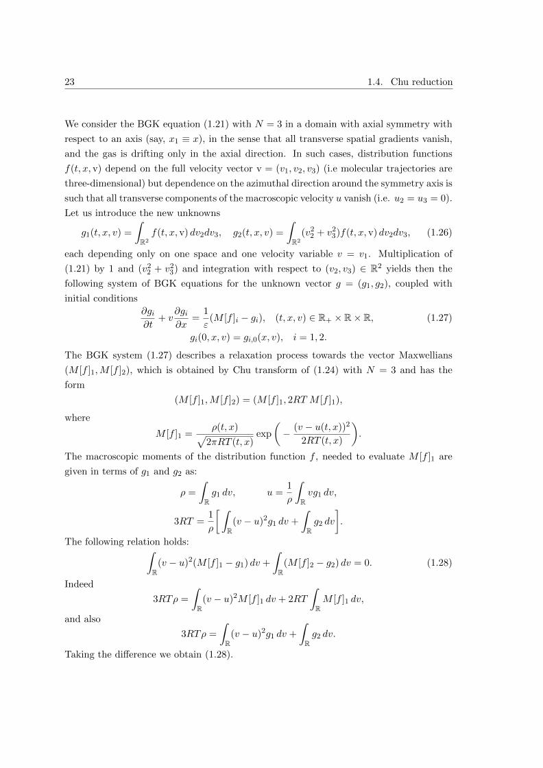
An interesting simplification that can be introduced into the BGK equation concerns, for
1D problem in space, the possibility to describe problems in 3D velocity space by means
of a system of two equations in one-dimensional velocity space. The idea is known as Chu
reduction [15] and can be applied under suitable symmetry assumptions.
23 1.4. Chu reduction
We consider the BGK equation (1.21) with N = 3 in a domain with axial symmetry with
respect to an axis (say, x1 ≡ x), in the sense that all transverse spatial gradients vanish,
and the gas is drifting only in the axial direction. In such cases, distribution functions
f(t, x, v) depend on the full velocity vector v = (v1, v2, v3) (i.e molecular trajectories are
three-dimensional) but dependence on the azimuthal direction around the symmetry axis is
such that all transverse components of the macroscopic velocity u vanish (i.e. u2 = u3 = 0).
Let us introduce the new unknowns
g1(t, x, v) =
∫
R2
f(t, x, v) dv2dv3, g2(t, x, v) =
∫
R2
(v22 + v2
3)f(t, x, v) dv2dv3, (1.26)
each depending only on one space and one velocity variable v = v1. Multiplication of
(1.21) by 1 and (v22 + v2
3) and integration with respect to (v2, v3) ∈ R2 yields then the
following system of BGK equations for the unknown vector g = (g1, g2), coupled with
initial conditions
∂gi∂t
+ v∂gi∂x
=1
ε(M [f ]i − gi), (t, x, v) ∈ R+ × R× R, (1.27)
gi(0, x, v) = gi,0(x, v), i = 1, 2.
The BGK system (1.27) describes a relaxation process towards the vector Maxwellians
(M [f ]1,M [f ]2), which is obtained by Chu transform of (1.24) with N = 3 and has the
form
(M [f ]1,M [f ]2) = (M [f ]1, 2RT M [f ]1),
where
M [f ]1 =ρ(t, x)√
2πRT (t, x)exp
(− (v − u(t, x))2
2RT (t, x)
).
The macroscopic moments of the distribution function f , needed to evaluate M [f ]1 are
given in terms of g1 and g2 as:
ρ =
∫
Rg1 dv, u =
1
ρ
∫
Rvg1 dv,
3RT =1
ρ
[ ∫
R(v − u)2g1 dv +
∫
Rg2 dv
].
The following relation holds:∫
R(v − u)2(M [f ]1 − g1) dv +
∫
R(M [f ]2 − g2) dv = 0. (1.28)
Indeed
3RTρ =
∫
R(v − u)2M [f ]1 dv + 2RT
∫
RM [f ]1 dv,
and also
3RTρ =
∫
R(v − u)2g1 dv +
∫
Rg2 dv.
Taking the difference we obtain (1.28).

Chapter 1. The Boltzmann equation and the BGK model 24
Chapter 2
Basic numerical methods for
evolutionary PDEs
In this chapter we will briefly recall some tools used in this thesis for the numerical
solution of the BGK equation. The semi-Lagrangian technique is inspired by the method of
characteristics for first order systems of linear PDEs. In order to derive a numerical method
from this general idea, several ingredients should be put together, mainly a technique for
ordinary differential equations to track characteristics, and a reconstruction technique to
recover pointwise values of the numerical solution. To this end, in the first part of this
chapter we present one-step and multi-step methods for ODEs, with particular attention to
Runge-Kutta and BDF methods. Then we present non oscillatory interpolation techniques,
such as ENO and WENO, needed in the numerical treatment of discontinuous solution
of evolutionary PDEs. Finally, the basic ideas of semi-Lagrangian schemes for PDEs are
presented.
2.1 Runge-Kutta methods for ODEs
We begin this section by introducing the generic numerical scheme for ODEs of first order1.
We have to numerically solve the following problem
y′ = g(t, y), g : R× Rm → Rm
y(0) = y0, t ∈ [0, T ]. (2.1)
This problem is well posed when g(t, y) is a Lipschitz function with respect to y, uniformly
in t. Fixed a time step ∆t, the continuous interval [0, T ] is replaced by a discrete point set
1A higher order equation may be always written as a first order system.
25
Chapter 2. Basic numerical methods for evolutionary PDEs 26
tn defined by tn = n∆t, n ∈ N. The numerical solution in this points will be denoted by
yn ' y(tn).
A numerical method is an equation that, starting from the discrete values yn+1−j , j =
0, ...k, k ∈ N, allows to evaluate the discrete solution at time tn+1. If k, the so-called step-
number, is equal to 1 the method is one-step, otherwise it is called a multi-step method.
In detail, we will examine Runge-Kutta schemes, that are a class of one-step methods,
and the Backward Differentiation Formulas (BDF) schemes, that belong to the multi-step
methods family.
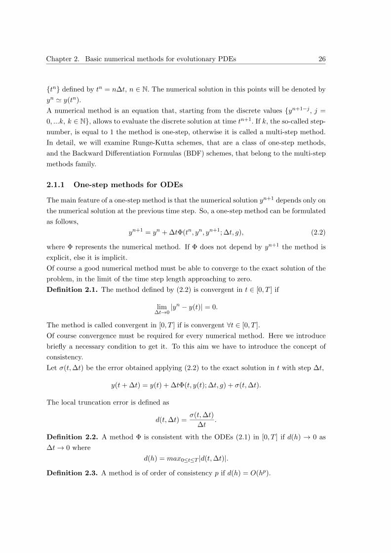
2.1.1 One-step methods for ODEs
The main feature of a one-step method is that the numerical solution yn+1 depends only on
the numerical solution at the previous time step. So, a one-step method can be formulated
as follows,
yn+1 = yn + ∆tΦ(tn, yn, yn+1; ∆t, g), (2.2)
where Φ represents the numerical method. If Φ does not depend by yn+1 the method is
explicit, else it is implicit.
Of course a good numerical method must be able to converge to the exact solution of the
problem, in the limit of the time step length approaching to zero.
Definition 2.1. The method defined by (2.2) is convergent in t ∈ [0, T ] if
lim∆t→0
|yn − y(t)| = 0.
The method is called convergent in [0, T ] if is convergent ∀t ∈ [0, T ].
Of course convergence must be required for every numerical method. Here we introduce
briefly a necessary condition to get it. To this aim we have to introduce the concept of
consistency.
Let σ(t,∆t) be the error obtained applying (2.2) to the exact solution in t with step ∆t,
y(t+ ∆t) = y(t) + ∆tΦ(t, y(t); ∆t, g) + σ(t,∆t).
The local truncation error is defined as
d(t,∆t) =σ(t,∆t)
∆t.
Definition 2.2. A method Φ is consistent with the ODEs (2.1) in [0, T ] if d(h) → 0 as
∆t→ 0 where
d(h) = max0≤t≤T |d(t,∆t)|.
Definition 2.3. A method is of order of consistency p if d(h) = O(hp).
27 2.1. Runge-Kutta methods for ODEs
Theorem 2.1.1. If the function Φ(t, y; ∆t) defines a consistent method in [0, T ] of order
p, and if it is Lipschitz ∀h ≤ h0, h0 > 0, then the method is convergent in [0, T ] with order
p.
2.1.2 Runge-Kutta methods
Runge-Kutta methods are an important family of implicit and explicit methods, which are
used in temporal discretization for the approximation of solutions of ordinary differential
equations.
In general, given a integer ν (number of stages), a ν-stage Runge-Kutta (RK) method has
the following form:
ki = g(tn + ci∆t, yn +
ν∑
j=1
aijkj) i = 1, ..., ν
yn+1 = yn + ∆t
ν∑
i=1
biki. (2.3)
In other words, a RK method is completely characterized through its Butcher’s table
c A
bT
where A = (aij) is a ν × ν matrix and c = (1, · · · , cν)T and b = (b1, · · · , bν)T are vectors.
ki are called RK fluxes. When aij = 0 for i ≥ j we have an explicit method (ERK).
If aij = 0 for i > j and at least one aii 6= 0, we have a diagonal implicit RK (DIRK)
method.In all other cases we speak of an implicit (IRK) method.
Usually, the coefficients satisfy the following relations:
ν∑
i=1
bi = 1 and ci =
ν∑
i=1
aij i = 1, ..., ν.
The first is a consistency condition and ensures that at least first order accuracy is achieved;
the second one greatly simplifies the derivation of order conditions for high order methods.
Definition 2.4. A Runge-Kutta method (2.3) has order p if for sufficiently smooth prob-
lems (2.1)
|y(t0 + ∆t)− y(1)| ≤ Chp+1,
i.e., if the Taylor series for the exact solution y(t0 + ∆t) and for y1 coincide up to (and
including) the term hp.
Chapter 2. Basic numerical methods for evolutionary PDEs 28
To recover the order conditions about the coefficients of the Butcher’s table we have to
compare the Taylor series for the exact and numerical solution. This part is very technical
and we refer to [27] for more details. Here are listed the conditions to achieve order 1, 2
and 3.
- First order condition:ν∑
i=1
bi = 1. (2.4)
- Second order condition:ν∑
i=1
bici =1
2. (2.5)
- Third order conditions:
ν∑
j=1
ν∑
i=1
biaijcj =1
6,
ν∑
i=1
bic2i =
1
3. (2.6)
Of course to obtain second and third order the conditions for the smaller order must
be satisfied. Thus, to obtain third order we have four conditions. The number of the
conditions grows with p. The construction of higher order RK formulas is not an easy
task. For instance, to achieve order 4, 5, 6, the number of conditions is respectively 8, 17,
37. Thus, to build a high order method one can increase the number ν of stages, but in
this way also the computational cost increases. Hence, one always tries to minimize the
number of intermediate stage.
Let us focus now on the stability properties of the RK methods.
2.1.3 Stability analysis for Runge-Kutta methods
Explicit methods
We consider the famous Dahlquist test equation
y′ = λy, y0 = 1, z = ∆tλ. (2.7)
Using a simple explicit Euler’s method to solve (2.7) we have
yn+1 = R(z)yn
with
R(z) = 1 + z.
29 2.1. Runge-Kutta methods for ODEs
Hence it is immediate to observe that the numerical solution yn+1 is bounded if the
argument z lies in the region
S = z ∈ C : |R(z)| < 1 = z ∈ C : |z + 1| ≤ 1
which is the circle of radius 1 and center (−1, 0) on the complex plane. The function
R(z) is called the stability function of the method. It can be interpreted as the numerical
solution after one step for (2.7). The set
S = z ∈ C : |R(z)| < 1 (2.8)
is called the stability domain of the method.
The following theorem can be proved:
Theorem 2.1.2. If an explicit RK methods is of order p, then
R(z) = 1 + z +z2
2!+ · · ·+ zp
p!+O(zp+1)
and if p = ν
R(z) = 1 + z +z2
2!+ · · ·+ zν
ν!. (2.9)
Implicit methods
Now, if we use the simple implicit Euler’s method to solve (2.7) we have
R(z) =1
1 + z.
This time, the stability domain is the exterior of the circle with radius 1 and center
(+1, 0). The stability domain thus covers the entire negative half-plane and a large part
of the positive half-plane as well. The implicit Euler method is thus more stable than the
explicit one.
Proposition 2.1.3. The ν-stage implicit RK method
ki = g(tn + ci∆t, yn +
ν∑
j=1
aijkj) i = 1, ..., ν
yn+1 = yn + ∆t
ν∑
i=1
biki
applied to (2.7) yields yn+1 = R(z)yn with
R(z) = 1 + zbT (I − zA)−1e,
where e = (1, ..., 1)T .
Chapter 2. Basic numerical methods for evolutionary PDEs 30
Moreover, can be proved that for implicit method the stability function satisfies
R(z) =det(I − zA+ zebT )
dat(I − zA). (2.10)
It is to observe immediately that the stability function is rational with numerator and
denominator of degree ≤ ν.The Dahlquist equation is stable if the eigenvalues λ lie on the entire complex half-plane
C−.Definition 2.5. A numerical method is said A-stable if the stability domain S is such
that S ⊇ C−.A RK method with (2.10) as stability function is A-stable if and only if
|R(iy)| ≤ 1, ∀y ∈ R
and R(z) is analytic for Re z < 0.
We have to notice that, by (2.9), an A-stable method must be implicit.
2.1.4 L-stability
Although some methods admit a stability region that coincides exactly with the negative
half-plane, not always these represent the best solution. This is due to the behavior of
the rational function R(z) when z →∞ in case of stiff problems. This phenomena can be
avoided if L-stability is required,
Definition 2.6. A numerical method is said L-stable if it is A-stable and
limz→∞
R(z) = 0.
A useful tool to construct an L-stable Runge-Kutta method is given by the following
theorem:
Theorem 2.1.4. If an implicit Runge-Kutta method with nonsingular A satisfies one of
the following conditions:
aνj = bj , j = 1, ..., ν, (2.11)
ai1 = b1, i = 1, ..., s,
then R(∞) = 0. This makes A-stable methods L-stable.
Methods satisfying (2.11) are called stiffly accurate.
31 2.2. Multi-step methods
2.2 Multi-step methods
The birth of multi-step methods is due mainly to J. C. Adams [27, 28]. In contrast
to one-step methods, where the numerical solution is obtained solely from the differen-
tial equation and the initial value, a multi-step approach consists of two parts: firstly, a
starting procedure which provides y1, ·, yn−1 at time t1, ·, tn−1, and, secondly, a multi-step
formula to obtain an approximation to the exact solution y(tn). There are several pos-
sibilities for obtaining the starting values. Adams actually computed them using Taylor
series expansion of the exact solution. Another possibility is to use any one-step method,
e.g. a Runge-Kutta method. It is also usual to start with low-order multi-step methods
and very small step size.
Two family of multi-step methods can be considered. One is based on numerical integra-
tion of the integral equation of (2.1) using some qradrature formula. The other one is
based on interpolation. The Adams methods belong to the former, instead, the Backward
Differentiation Formulas (BDF) methods belong to the latter one.
2.2.1 Adams methods
We suppose that the solution is known at time tn, · · · , tn−q and we wants the numerical
solution yn+1 at time tn+1. We consider (2.1) in integrated form,
y(tn+k) = y(tn−j) +
∫ tn+k
tn−jg(t, y(t)) dt. (2.12)
On the right hand of (2.12) appears the unknown solution y(t). But since the approxima-
tions yn, · · · , yn−q are known, the values gi = g(ti, yi) for i = n−q, · · · , n are also available
and it is natural to replace the function g(t, y(t)) in (2.12) by the interpolation polynomial
of degree q through the points (ti, yi), for i = n − q, · · · , n. Skipping the technical steps,
available in [27], one obtain the following general form for the Adams multi-steps methods
yn+k = yn−j + ∆t
q∑
i=0
βign−i. (2.13)
Varying the values of k and j, the Adams methods achieve different features and names:
j = 0, k = 1 : explicit Adams or Adams-Bashforth methods;
j = 1, k = 0 : implicit Adams or Adams-Moulton methods;
j = 1, k = 1 : Nystrom methods (explicit methods);
j = 2, k = 0 : Milne methods (implicit methods).
Chapter 2. Basic numerical methods for evolutionary PDEs 32
2.2.2 BDF methods
The Backward Differentiation Formulas (BDF) methods are linear implicit multi-step
methods that, for a given function and time, approximate the derivative of that func-
tion using information from already computed times by interpolation, thereby increasing
the accuracy of the approximation. These methods are especially used for the solution of
stiff differential equations.
Assume that the approximation yn+1−q, ..., yn to the exact solution of (2.1) are known. In
order to derive a formula for yn+1, we consider the polynomial p(t) which interpolates the
values (ti, yi) | i = n− q + 1, ..., n+ 1. The unknown value yn+1 will now be determined
in such a way that the polynomial p(t) satisfies the differential equation at tn+1, i.e.
q′(tn+1) = g(tn+1, yn+1).
Skipping the details, present in [27], the general form of the BDF method is
q∑
i=0
αiyn+1−i = ∆tg(tn+1, yn+1). (2.14)
For the sake of completeness we give the formulas related to q = 1, 2, 3 :
q = 1, yn+1 − yn = ∆tg(tn+1, yn+1), (2.15)
q = 2,3
2yn+1 − 2yn +
1
2yn−1 = ∆tg(tn+1, yn+1), (2.16)
q = 3,11
6yn+1 − 3yn +
3
2yn−1 − 1
3yn−2 = ∆tg(tn+1, yn+1). (2.17)
2.2.3 Local error and order conditions
The general theory of multi-step methods studies the following difference equation
q∑
i=0
αiyn+i = ∆t
q∑
i=0
βign+i, (2.18)
which includes all previously considered methods as special cases.
Definition 2.7. The local error d(y, t,∆t) of the multi-step method (2.18) is defined by
d(y, t,∆t) = |y(tn+1)− yn+1|,
where y(t) is the exact solution of (2.1) and yn+1 the numerical solution obtained from
(2.18).
33 2.2. Multi-step methods
Once the local error of a multistep method is defined, one can introduce the concept of
order in the same way as for one-step methods.
Definition 2.8. The multi-step method (2.18) is said to be of order p if for all sufficiently
regular functions y(t), we have
d(y, t,∆t) = O(∆tp+1).
Our next aim is to characterize the order of a multi-step method in terms of the free
parameters αi and βi. Dahlquist was the first to observe the fundamental role of the
polynomials
ρ(z) =
q∑
i=0
αizi, σ(z) =
q∑
i=0
βizi.
They will be called the generating polynomials of the multi-step method (2.18).
Theorem 2.2.1. The multi-step method (2.18) is of order p, if and only if one of the
following equivalent conditions is satisfied:
∑qi=0 αi = 0 and
∑qi=0 αii
k = k∑q
i=0 βiik−1 for k = 1, · · · , p;
ρ(e∆t)−∆tσ(e∆t) = O(∆tp+1) for ∆t→ 0;
ρ(z)
ln z− σ(z) = O((z − 1)p) for z → 1.
Remark 1. The conditions for a multi-step method to be of order 1, which are usually
called consistency conditions, can also be written in the form
ρ(1) = 0, ρ′(1) = σ(1).
2.2.4 Stability and the first Dahlquist barrier
High order and a small local error are not sufficient for a useful multi-step method. The
numerical solution can be unstable even though the step size ∆t is taken very small. The
essential part is the behavior of the solution as n→∞ (or ∆t→ 0) with n∆t fixed. From
(2.18) for ∆t→ 0 we obtain
αqyn+q + αq−1y
n+q−1 + · · ·+ α0 = 0. (2.19)
This can be interpreted as the numerical solution of the method (2.18) for the differential
equation
y′ = 0.
We put yj = zj in (2.19), divide by zn, and find that z must be a root of ρ(z).
Chapter 2. Basic numerical methods for evolutionary PDEs 34
Lemma 2.2.2. Let z1, · · · , zl be the roots of ρ(z), of respective multiplicity m1, · · · ,ml.
Then the general solution of (2.19) is given by
yn = p1(n)zn1 + · · ·+ pl(n)znl (2.20)
where the pj(n) are polynomials of degree mj − 1.
Formula (2.20) shows us that for boundedness, and therefore stability, of yn, as n → ∞,we need that the roots of ρ(z) lie in the unit disc and that the roots on the unit circle are
simple.
Definition 2.9. The multi-step method (2.18) is called zero-stable if the generating poly-
nomial ρ(z) satisfies the root conditions; i.e.
- The roots of ρ(z) lie on or within the unit circle;
- The roots on the unit circle are simple.
The following theorem can be proved about the relation between the stability of multi-step
methods and accuracy order.
Theorem 2.2.3. The k-step BDF formula (2.14) is stable for q ≤ 6, and unstable for
q ≥ 7.
Theorem 2.2.4 (The first Dahlquist barrier). The order p of a stable linear q-step method
satisfies
p ≤ q + 2 if q is even,
p ≤ q + 1 if q is odd,
p ≤ q if βq/αq ≤ 0 (in particular if the method is explicit.)
2.2.5 A-Stability for multi-step methods
If we applied method (2.18) to the Dahlquist’s test function y′ = λy we obtain
(αk − µβk)yn+k + · · ·+ (α0 − µβ0)yn = 0, µ = λ∆t. (2.21)
The characteristic equation of the difference equation (2.21) is therefore
ρ(z)− µσ(z) = 0, (2.22)
which depends on the complex parameter µ. The difference equation (2.21) has stable
solutions iff all roots of (2.22) are ≤ 1 in modulus. In addition, multiple roots must be
strictly smaller than 1. We therefore formulate
Definition 2.10. The set S of µ ∈ C such that all roots zj(µ) of (2.22) satisfy |zj(µ)| ≤ 1
and multiple roots satisfy |zj(µ)| < 1, is called the stability domain or region of absolute
stability of method (2.18).
35 2.3. High order non oscillatory reconstruction
Definition 2.11. A multi-step method of the form (2.18) is A-stable if S ⊇ C−.BDF methods are A-stable only for q ≤ 2, see [28]. For q = 3, 4, 5 and 6, we see that the
methods loose more and more stability, even if for q = 3 only a very small part of C− in
not included in the region of the absolute stability. For q ≥ 7, as we know, the formulas
are unstable anyway.
2.3 High order non oscillatory reconstruction
The new class of numerical methods to solve the BGK model of the Boltzmann equation,
that we will introduce in Chapter 3, is based on a semi-Lagrangian formulation of (1.21)-
(1.24). As we will see in the next sections, this formulation permits in principle to solve
the problem along characteristics, by tracking them back until the initial time. The feet of
characteristics generally will not be grid nodes, so interpolation is needed to reconstruct
the distribution function from the values on the grid nodes. In this section we are going
to introduce the numerical reconstruction adopted.
In order to obtain high order accuracy and to ensure the shock capturing properties of the
proposed schemes near the fluid regime, a suitable nonlinear reconstruction technique for
the computation of the numerical solution outside grid points is required. The numerical
technique used, developed in [11], is based on a ENO (Essential Non-Oscillatory) tech-
nique reconstruction. As the name suggests, their development is due to the necessity to
reconstruct a function, given by a discrete set of data, which exhibits discontinuity. In this
case in fact classical high order Lagrange interpolation methods are oscillatory. Of course,
these oscillations lead to numerical instability. Different ways have been proposed in the
past to solve this problem. One consists in the introduction of artificial viscosity to reduce
the oscillations, but this affects the solutions of the problems. Another way consists in the
use of slope limiters [34]. In this case the goal was to eliminate the oscillations completely.
The greater disadvantage of this method is that accuracy decreases to first order near the
discontinuity. ENO (essentially non oscillator) and WENO (weighted ENO) methods [53]
prevent formation of oscillations, still guaranteeing high order accuracy. Both methods are
based on the reconstruction of piecewise smooth functions by choosing the interpolation
points on smooth side of the function.
The original ENO and WENO techniques proposed by Shu [53], starting from the cell
averages values of the unknown function, aims to reconstruct the unknown function at cell
boundaries. Since we are interested in reconstruction for a generic point of the grid, we
refer to WENO reconstruction developed by Carlini, Ferretti and Russo [11] by reporting
Chapter 2. Basic numerical methods for evolutionary PDEs 36
the general framework for its implementation. In the following sections we introduce this
techniques.
2.3.1 The ENO approximation
Let us assume there is a smooth function u(x), and we know only its cell averages uj.Then we want to construct in each cell j a polynomial pj of a given degree m − 1 (i.e.
pj ∈ Πm−1)
pj(x) = u(x) +O(∆xm). (2.23)
In particular, we shall be interested in evaluating this polynomial at cell boundaries:
u−j+1/2 = pj(xj+1/2),
u+j−1/2 = pj(xj−1/2).
Such polynomial is constructed as follows. Take m adjacent cells, that include cell j. Let
these cells be denoted by j − r, j − r + 1, · · · , j + s with r + s + 1 = m, r, s ≥ 0. Then
impose that
〈pj〉l = 〈u〉l =1
∆x
∫ xl+1/2
xl−1/2
u(x) dx, l = j − r, · · · , j + s. (2.24)
These m independent conditions uniquely determine a polynomial of degree m − 1. Let
us show that indeed this polynomial satisfies condition (2.23). This is easily shown by
defining
U(x) ≡∫ x
au(x) dx,
a primitive of u(x). The left bound a is not relevant. We choose it so that a = xja−1/2. At
the right edge of cell i one has:
U(xi+1/2) = ∆xi∑
j=ja
uj .
Let Pj(x) ∈ Πm, and let Pj(xi+1/2) = U(xi+1/2), i = j − r − 1, · · · , j + s. These m + 1
conditions uniquely determine Pj ∈ Πm. Furthermore, from interpolation theory, one has
P (x) = U(x) +O(∆xm+1),
and therefore
p(x) = P ′(x) = U ′(x) +O(∆xm) = u(x) +O(∆xm).
Polynomial p(x) therefore satisfies (2.23) and (2.24).
There are m such polynomials. For example, for a polynomial of degree 2 one can choose
37 2.3. High order non oscillatory reconstruction
cells j − 2, j − 1, j, or j − 1, j, j + 1, or j, j + 1, j + 2. Which one should be chosen for
the reconstruction? This is exactly where ENO comes into play. First, observe that for
a given stencil, polynomial P (x) can be computed using the divided difference of the
function U(x) :
U [xi−1/2,xi+1/2] =
U(xi+1/2)− U(xi−1/2)
xi+1/2 − xi−1/2= ui,
therefore first and higher order divided differences of U can be computed by uj, without
using function U explicitly. Likewise, computation of p(x) can be performed using divided
differences that make use only of uj. The main purpose of the primitive function U(x)
is to find the proper stencil. The idea of ENO construction is the following. Take cell j,
and construct a linear function between point (xj−1/2, U(xj−1/2)) and (xj+1/2, U(xj+1/2)).
Let us call it P1(x). Then add one point, either to the left obtaining
R(x) = P1(x) + U [xj−3/2, xj−1/2, xj+1/2](x− xj−1/2)(x− xj+1/2),
or on the right, obtaining
R(x) = P1(x) + U [xj−1/2, xj+1/2, xj+3/2](x− xj−1/2)(x− xj+1/2).
Then choose the one which is less oscillatory, i.e. the one with the smallest second deriva-
tive. Therefore, extend your stencil by:
r → r + 1 if |U [xj−3/2, xj−1/2, xj+1/2]| < |U [xj−1/2, xj+1/2, xj+3/2]|,
or
s→ s+ 1 if |U [xj−3/2, xj−1/2, xj+1/2]| > |U [xj−1/2, xj+1/2, xj+3/2]|.Then one can repeat the procedure by adding one more point to the stencil, either to the
left or to the right, comparing the size of the next divided difference. The net effect of
this procedure will be to choose a stencil that uses the smooth part of the function in the
reconstruction.
For a given degree m−1, there are m possible stencils. For each of them there are two sets
of coefficients [53], cri, cri that compute u−j+1/2 and u+j−1/2 as a linear combination of
cell averages on the stencil. These coefficients can be computed once and used later. Once
the stencil is chosen (i.e. r is defined) by the ENO procedure, then one knows which set
of coefficients cri one has to use. The expression for u−j+1/2 and u+j−1/2 for each choice of
the stencil are of the form
u−j+1/2 =
m−1∑
i=0
criuj−r+1,
u+j−1/2 =
m−1∑
i=0
criuj−r+1.
Chapter 2. Basic numerical methods for evolutionary PDEs 38
2.3.2 The WENO approximation
In the ENO reconstruction one chooses a stencil with m nodes to construct a polynomial
of degree m − 1, in order to reach an accuracy of O(∆xm) in the cell. However, the
total number of points involved is 2m − 1. With all these points, a much more accurate
reconstruction is possible. Suppose, for the sake of argument, that m = 3, and that we
use a parabola to reconstruct the function u(x) in the cell j. Let qk denotes the parabola
obtained by matching the cell average in cells k − 1, k, k + 1, i.e. qk(x) is obtained by
imposing
〈qk〉l = ul, l = k − 1, k, k + 1.
Then for our polynomial pj ∈ Π2 we can use either qj−1, qj , or qj+1. Each choice would
give us third order accuracy. We could also choose a convex combination of qk,
pj = ωj−1qj−1 + ωj0qj + ωj1qj+1,
with ωj−1 +ωj0 +ωj1 = 1, ωjl ≥ 0, l = −1, 0, 1. Every such convex combination would provide
at least third order accuracy.
We can choose the weights according to the following requirements:
i) in the region of regularity of u(x) the values of the weights are chosen in such a way
to have a reconstruction of the function at some particular point with higher order
of accuracy. Typically we need high order accuracy at points xj + ∆x2 and xj − ∆x
2 .
With two more degrees of freedom it is possible to obtain fifth order accuracy at
point xj+1/2 (instead of third order).
We shall denote by C+−1, C
+0 , C
+1 the constants that provide high order accuracy at
point xj+1/2 :
pj(xj+1/2) =1∑
k=−1
C+k qj+k(xj+1/2) = u(xj+1/2) +O(h5),
and C−k , k = −1, 0, 1 the corresponding constants for high order reconstruction at
point xj−1/2,
pj(xj−1/2) =
1∑
k=−1
C−k qj+k(xj−1/2) = u(xj−1/2) +O(h5).
The value of these constants can be computed, and are given by
C+1 = C−−1 =
3
10, C+
0 = C−0 =3
5, C+
−1 = C−1 =1
10.
39 2.3. High order non oscillatory reconstruction
ii) in the region near a discontinuity, one should make use only of the values of the cell
averages that belong to the regular part of the profile.
This is obtained by making the weights depend on the regularity of the function in the
corresponding cell. In WENO scheme this results in setting
αjk =Ck
(βjk + δ)2, k = −1, 0, 1,
and
ωjk =αjk∑l α
jl
,
with δ a properly small parameter, usually of order 10−6. Here βk are the so called
smoothness indicators, and are used to measure the smoothness or, more precisely, the
roughness of the function, by measuring some weighted norm of the function and its
derivatives. Typically
βjk =2∑
l=1
∫ xj+1/2
xj−1/2
∆x2l−1
(dlqj+k(x)
dxl
)2
dx, k = −1, 0, 1.
The integration can be carried out explicitly, obtaining
β−1 =13
12(uj−2 − 2uj−1 + uj)
2 +1
4(uj−2 − 4uj−1 + 3uj)
2,
β0 =13
12(uj−1 − 2uj + uj+1)2 +
1
4(uj−1 − uj+1)2,
β1 =13
12(uj − 2uj+1 + uj+2)2 +
1
4(3uj − 4uj+1 + uj+2)2.
With three parabolas one obtains a reconstruction that gives up to fifth order accuracy in
smooth region, and that degrades to third order near discontinuities. A detailed descrip-
tion of ENO and WENO reconstruction can be found in the Chapter 4 of [53].
2.3.3 General WENO reconstruction
In the previous sections the WENO reconstruction method has been introduced. This
allows us to obtain a non oscillatory high order interpolation near particular points of the
computational grid, the cell boundary. Now the question concerns the WENO method for
a generic point of the grid. To this aim we refer to a recent result by Carlini, Feretti and
Russo [11]. In the following two sections we present as the second-third (WENO23) and
the third-fifth (WENO35) order interpolation work.
Chapter 2. Basic numerical methods for evolutionary PDEs 40
2.3.4 Second-third order WENO interpolation (WENO23)
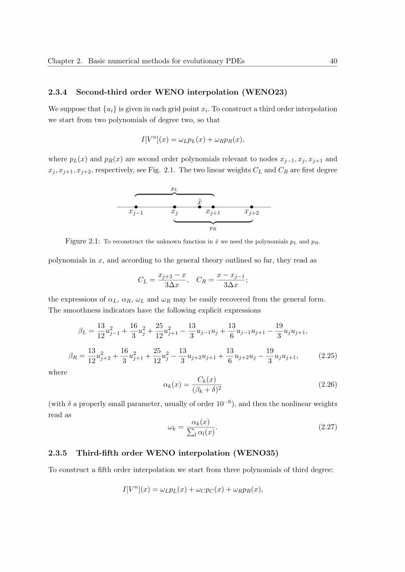
We suppose that ui is given in each grid point xi. To construct a third order interpolation
we start from two polynomials of degree two, so that
I[V n](x) = ωLpL(x) + ωRpR(x),
where pL(x) and pR(x) are second order polynomials relevant to nodes xj−1, xj , xj+1 and
xj , xj+1, xj+2, respectively, see Fig. 2.1. The two linear weights CL and CR are first degree
xj−1 xj xj+1 xj+2
x
pL︷ ︸︸ ︷
︸ ︷︷ ︸pR
Figure 2.1: To reconstruct the unknown function in x we need the polynomials pL and pR.
polynomials in x, and according to the general theory outlined so far, they read as
CL =xj+2 − x
3∆x, CR =
x− xj−1
3∆x;
the expressions of αL, αR, ωL and ωR may be easily recovered from the general form.
The smoothness indicators have the following explicit expressions
βL =13
12u2j−1 +
16
3u2j +
25
12u2j+1 −
13
3uj−1uj +
13
6uj−1uj+1 −
19
3ujuj+1,
βR =13
12u2j+2 +
16
3u2j+1 +
25
12u2j −
13
3uj+2uj+1 +
13
6uj+2uj −
19
3ujuj+1, (2.25)
where
αk(x) =Ck(x)
(βk + δ)2(2.26)
(with δ a properly small parameter, usually of order 10−6), and then the nonlinear weights
read as
ωk =αk(x)∑l αl(x)
. (2.27)
2.3.5 Third-fifth order WENO interpolation (WENO35)
To construct a fifth order interpolation we start from three polynomials of third degree:
I[V n](x) = ωLpL(x) + ωCpC(x) + ωRpR(x),
41 2.4. Semi-Lagrangian schemes
where the third order polynomials pL(x), pC(x) and pR(x) are constructed, respectively,
on xj−2, xj−1, xj , xj+1, on xj−1, xj , xj+1, xj+2, and on xj , xj+1, xj+2, xj+3. The weights
CL, CC and CR are second degree polynomials in x, and have the form
CL =(x− xj+2)(x− xj+3)
20∆x2, CC = −(x− xj−2)(x− xj+3)
10∆x2,
CR =(x− xj−2)(x− xj−1)
20∆x2,
while the smoothness indicators βC and βR have the expressions
βC =61
45u2j−1 +
331
30u2j +
331
30u2j+1 +
61
45u2j+2 −
141
20uj−1uj +
179
30uj−1uj+1
−293
180uj−1uj+2 −
1259
60ujuj+1 +
179
30ujuj+2 −
141
20uj+1uj+2,
βR =407
90u2j +
721
30u2j+1 +
248
15u2j+2 +
61
45u2j+3 −
1193
60ujuj+3 +
439
30ujuj+2
−683
180ujuj+3 −
2309
60uj+1uj+2 +
309
30uj+1uj+3 −
553
60uj+2uj+3,
and βL can be obtained using the same set of coefficients of βR in a symmetric way (that
is, replacing the indices j−2, · · · , j+3 with j+3, · · · , j−2) and αk and ωk are computed
as in (2.26) and in (2.27).
2.4 Semi-Lagrangian schemes
The semi-Lagrangian technique for the approximation of first-order partial differential
equations is based on the method of characteristics for advection equation, which ac-
counts for the flow of information in the model equation.
At the numerical level, the semi-Lagrangian approximation mimics the method of char-
acteristics, looking for the foot of the characteristic curve passing through every node,
and following this curve for a single time step. This procedure provides methods which
are unconditionally stable with respect to the choice of the time step. In this section we
present this approach through some model problems.
A basic and very intuitive example to show as the semi-Lagrangian formulation works is
the linear advection equation:
ut(t, x) + f(t, x) · ux(u, x) = g(t, x), (t, x) ∈ (t0, T )× R. (2.28)
Here, f : (t0, T )×R→ R is the drift term and g : (t0, T )×R→ R is the source term. We
look for a solution u : (t0, T )× R→ R satisfying the initial condition
u(t0, x) = u0(x), x ∈ R. (2.29)
Chapter 2. Basic numerical methods for evolutionary PDEs 42
This is a classical model describing the transport of a scalar field, e.g. the distribution
of a pollutant emitted by one of more sources (represented by g), and transported by a
water stream or a wind (represented by f).
The physical interpretation is better clarified through the method of characteristics which
provides an alternative characterization of the solution. In the simplest case, for g(t, x) = 0
and f(t, x) = c (constant) the solution is given by the well known representation formula
u(t, x) = u0(x− c(t− t0)) (t, x) ∈ (t0, T )× R. (2.30)
In fact, assume that a regular solution u exists. Differentiating u with respect to t along
a curve of the form (t, y(t)), we obtain
d
dtu(t, y(t)) = ux(t, y(t)) · y(t) + ut(t, y(t)), (2.31)
so that, since u solves the advection equation, the total derivative (2.31) will identically
vanish along the curves which satisfy
y(t) = c.
Such curves have the physical meaning of flow lines along which the scalar field u is
transported. They are known as characteristics and, in this particular case, are straight
lines. Then, to assign a value to the solution at a point (t, x) it suffices to follow the
unique line passing through (t, x) until it crosses the x-axis at the point z = x− c(t− t0),
z being the foot of the characteristic. Since the solution is constant along this line, we get
expression (2.30). Conversely, it is easy to check that a function of x and t in the form
(2.30) satisfies with (2.28) f(t, x) = c and g(t, x) = 0, provided u0 is differentiable.
2.4.1 Simple semi-Lagrangian examples of approximation schemes
Now we try to give some basic ideas (in a single space dimension) about the approxima-
tion schemes for the model problems introduced above, the linear advection equation at
constant speed c (to fix ideas, we assume that c > 0):
ut + cux = 0 (t, x) ∈ (0, T )× R
u(0, x) = u0(x) x ∈ R.(2.32)
The more classical method to construct an approximation of (2.32) is to build a uniform
grid in space and time (a lattice) with constant steps ∆x and ∆t, covering the domain of
the solution: (tn, xj) = (n∆t, j∆x), n ∈ N, n ≤ T
∆t, j ∈ Z
.
43 2.4. Semi-Lagrangian schemes
The basic idea behind all finite difference approximation is to replace every derivative by
an incremental ratio. Thus, one obtains a finite dimensional problem whose unknowns are
the values of the numerical solution at all the nodes of the lattice, so that the value unjassociated to the node (tn, xj) should be regarded as an approximation of u(tn, xj). For
the time derivative, it is natural to choose the forward incremental ratio
ut(t, x) =u(t+ ∆t, x)− u(t, x)
∆t
which allows, starting from the solution at the initial time t0, to compute explicitly the
approximations for increasing times tk > t0. Writing the forward incremental ratio in time
at (tn, xj), we get
ut(tn, xj) '
un+1j − unj
∆t. (2.33)
For the approximation of ux we have several possibilities, like
ux(tn, xj) 'unj+1 − unj
∆x(right finite difference)
ux(tn, xj) 'unj − unj−1
∆x(left finite difference)
ux(tn, xj) 'unj+1 − unj−1
2∆x(centered finite difference)
which are all based on the values at the nodes (tn, xk).
In this case , the choice of the approximation for ux crucially affects the convergence of
the numerical solution to the exact solution. Although centered finite difference would
in principle provide a more accurate approximation of the space derivative, given the
time derivative approximation (2.33), the only choice which leads to a convergent scheme
[33, 34] is to use the left incremental ratio if c > 0, the right incremental ratio if c < 0,
which corresponds to the so-called upwind scheme. In conclusion, for c > 0, we obtain a
scheme in the formun+1j − unj
∆t+ c
unj − unj−1
∆x= 0. (2.34)
A different way to construct the approximation of (2.32) is to consider the advection term
as a directional derivative and write
cux(tn, xj) ' −un(xj − cδ)− unj
δ
where δ is a small positive parameter, and un denotes an extension of the numerical
solution (at time tn) to be computed outside the grid points. Coupling the forward finite
Chapter 2. Basic numerical methods for evolutionary PDEs 44
difference in time with this approximation we get
un+1j − unj
∆t−un(xj − cδ)− unj
δ= 0,
and finally, choosing δ = ∆t, we obtain the scheme
un+1j = un(xj − c∆t). (2.35)
This is the semi-Lagrangian scheme for (2.32), which could also be deduced from a dis-
cretization of the representation formula (2.30). Contrary to finite difference approach,
semi-Lagrangian schemes use points which may not be grid nodes (xj − c∆t in our ex-
ample), thus the corresponding values of the numerical solution need to be reconstructed
by some interpolation technique. In section 2.3 we have already presented the high order
interpolation techniques used to achieve high order semi-Lagrangian numerical schemes
developed in chapter 3.
2.4.2 CFL condition for semi-Lagrangian schemes
In 1928, long time before the theory of convergence of numerical schemes for PDEs had
become an established matter, Courant, Friedrichs and Lewy published a paper in which
the concept of domain of dependence [33, 34, 48] was singled out as a key point for the
convergence of numerical schemes. To sketch the general idea, we first define the analytical
domain of dependence Dd(t, x) of the solution u at a point (t, x), as the smallest set such
that, if the initial condition u0 of (2.32) is changed on the set RdrDd(t, x), u(t, x) remains
unchanged. The discrete counterpart of this set is the numerical domain of dependence
D∆d (t, x), for a point (t, x) = (tn, xi) in the space-time grid, which is the set of all nodes
xj such that u0(xj) affects the value uni .
The Courant, Friedrichs and Lewy (CFL) condition states that, for any point (t, x), the
condition that the analytical domain of dependence must be included in the numerical
domain of dependence, is a necessary condition for stability.
The proof of the CFL condition is very simple: if the analytical domain of dependence is
not included in the numerical one, then there exist a subset of Dd(t, x) which have non
intersection with D∆d (t, x). Therefore, since any change in the value of u0 in this subsets
modifies the value of u(t, x) but not the value of the numerical approximation, the scheme
cannot be convergent.
On the other hand, by the Lax equivalence theorem (which was stated about thirty years
later) [33, 34] the CFL condition is also a necessary condition for stability. Indeed, since
a consistent scheme is convergent if and only if it is stable, if a consistent scheme violates
45 2.4. Semi-Lagrangian schemes
the CFL condition, then this scheme is unstable.
One of the most interesting advantages of the numerical schemes based on a semi-Lagrangian
formulation is that they allow to achieve stability without strict restrictions on the time
step.
If we look at the upwind scheme (2.34), that can be written in the following way:
un+1j = unj − c
∆t
∆x(unj − unj−1), (2.36)
we can observe that the numerical domain of dependence is composed by xj and xj−1. The
analytical one depends on the choice of the time step. A relative big time step could take
the foot of characteristic with velocity c > 0 outside the grid cell [xj−1, xj ], and therefore
could violate the CFL condition. So, intuitively, the CFL condition for the upwind scheme
states thatc∆t
∆x< 1 ⇔ ∆t <
∆x
c. (2.37)
The stability of the scheme can be checked in various ways. A rigorous one that can be
used, since the equation and method are linear, is Fourier analysis. We look for a solution
of the form
unj = ρneijξ, (2.38)
where i =√−1 denotes the imaginary unit. Assume c > 0. Then, substituting (2.38) in
(2.36) we have
ρ = 1− ∆t
∆xc(1− eiξ)
= 1− λ(1− cosξ)− iλ sin ξ,
where λ = c∆t/∆x. Performing the calculations one has
|ρ|2 = 1− 2λ(1− λ)(1− cosξ).
Because 1− cosξ ≥ 0 and λ > 0, it is |ρ|2 < 1 if 1− λ > 0, and therefore if λ < 1 that is
the same of (2.37).
So, if we introduce the Courant number, denoted by CFL, the upwind scheme is stable if
∆t = CFL∆x
c,
where CFL< 1.
In the same way, we can compute the CFL condition for the semi-Lagrangian scheme
for the advection equation expressed by (2.35). As we can see, in this case the numerical
Chapter 2. Basic numerical methods for evolutionary PDEs 46
domain of dependence is composed by xj and by the foot of the characteristics xj − c∆t.Therefore, in this case, the numerical domain of dependence is not fixed, but depends on
c and ∆t. In this way the analytical domain of dependence will be always included in the
numerical one, and to achieve numerical stability there is no need for restrictions on time
step choice.
This is the more relevant feature of numerical schemes based on a semi-Lagrangian for-
mulation. The possibility to choose CFL numbers greater than one or more, without
losing stability properties, makes them very interesting from a computational point of
view, because the computational cost decreases substantially.
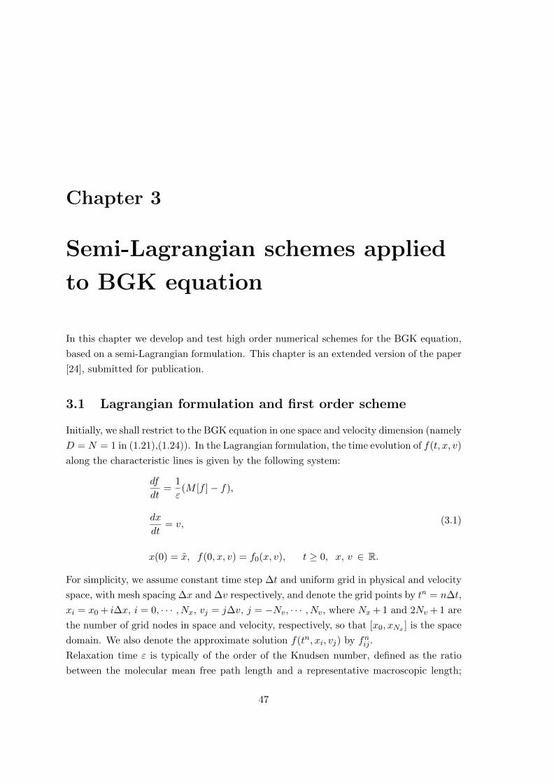
Chapter 3
Semi-Lagrangian schemes applied
to BGK equation
In this chapter we develop and test high order numerical schemes for the BGK equation,
based on a semi-Lagrangian formulation. This chapter is an extended version of the paper
[24], submitted for publication.
3.1 Lagrangian formulation and first order scheme
Initially, we shall restrict to the BGK equation in one space and velocity dimension (namely
D = N = 1 in (1.21),(1.24)). In the Lagrangian formulation, the time evolution of f(t, x, v)
along the characteristic lines is given by the following system:
df
dt=
1
ε(M [f ]− f),
dx
dt= v,
x(0) = x, f(0, x, v) = f0(x, v), t ≥ 0, x, v ∈ R.
(3.1)
For simplicity, we assume constant time step ∆t and uniform grid in physical and velocity
space, with mesh spacing ∆x and ∆v respectively, and denote the grid points by tn = n∆t,
xi = x0 + i∆x, i = 0, · · · , Nx, vj = j∆v, j = −Nv, · · · , Nv, where Nx + 1 and 2Nv + 1 are
the number of grid nodes in space and velocity, respectively, so that [x0, xNx ] is the space
domain. We also denote the approximate solution f(tn, xi, vj) by fnij .
Relaxation time ε is typically of the order of the Knudsen number, defined as the ratio
between the molecular mean free path length and a representative macroscopic length;
47
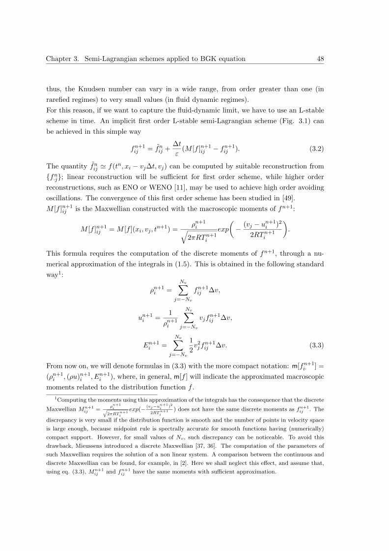
Chapter 3. Semi-Lagrangian schemes applied to BGK equation 48
thus, the Knudsen number can vary in a wide range, from order greater than one (in
rarefied regimes) to very small values (in fluid dynamic regimes).
For this reason, if we want to capture the fluid-dynamic limit, we have to use an L-stable
scheme in time. An implicit first order L-stable semi-Lagrangian scheme (Fig. 3.1) can
be achieved in this simple way
fn+1ij = fnij +
∆t
ε(M [f ]n+1
ij − fn+1ij ). (3.2)
The quantity fnij ' f(tn, xi − vj∆t, vj) can be computed by suitable reconstruction from
fn·j; linear reconstruction will be sufficient for first order scheme, while higher order
reconstructions, such as ENO or WENO [11], may be used to achieve high order avoiding
oscillations. The convergence of this first order scheme has been studied in [49].
M [f ]n+1ij is the Maxwellian constructed with the macroscopic moments of fn+1:
M [f ]n+1ij = M [f ](xi, vj , t
n+1) =ρn+1i√
2πRTn+1i
exp
(− (vj − un+1
i )2
2RTn+1i
).
This formula requires the computation of the discrete moments of fn+1, through a nu-
merical approximation of the integrals in (1.5). This is obtained in the following standard
way1:
ρn+1i =
Nv∑
j=−Nvfn+1ij ∆v,
un+1i =
1
ρn+1i
Nv∑
j=−Nvvjf
n+1ij ∆v,
En+1i =
Nv∑
j=−Nv
1
2v2j f
n+1ij ∆v. (3.3)
From now on, we will denote formulas in (3.3) with the more compact notation: m[fn+1i· ] =
(ρn+1i , (ρu)n+1
i , En+1i ), where, in general, m[f ] will indicate the approximated macroscopic
moments related to the distribution function f .
1Computing the moments using this approximation of the integrals has the consequence that the discrete
Maxwellian Mn+1ij =
ρn+1i√
2πRTn+1i
exp(− (vj−un+1i )2
2RTn+1i
) does not have the same discrete moments as fn+1ij . The
discrepancy is very small if the distribution function is smooth and the number of points in velocity space
is large enough, because midpoint rule is spectrally accurate for smooth functions having (numerically)
compact support. However, for small values of Nv, such discrepancy can be noticeable. To avoid this
drawback, Mieussens introduced a discrete Maxwellian [37, 36]. The computation of the parameters of
such Maxwellian requires the solution of a non linear system. A comparison between the continuous and
discrete Maxwellian can be found, for example, in [2]. Here we shall neglect this effect, and assume that,
using eq. (3.3), Mn+1ij and fn+1
ij have the same moments with sufficient approximation.
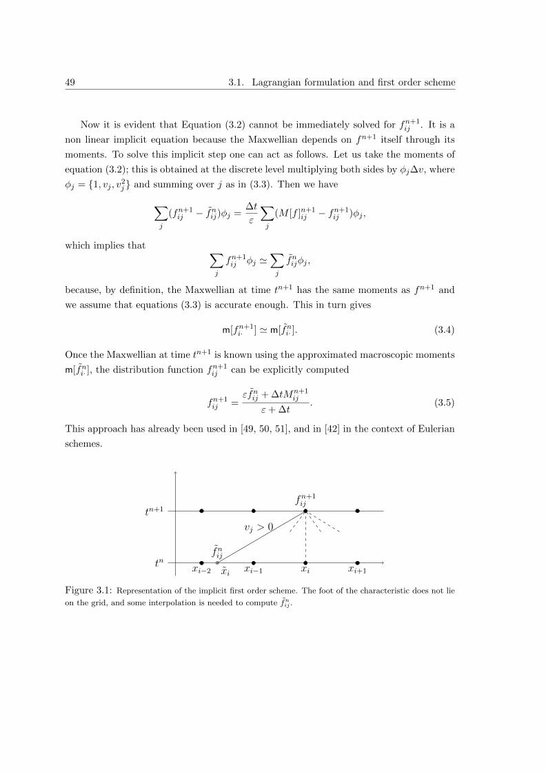
49 3.1. Lagrangian formulation and first order scheme
Now it is evident that Equation (3.2) cannot be immediately solved for fn+1ij . It is a
non linear implicit equation because the Maxwellian depends on fn+1 itself through its
moments. To solve this implicit step one can act as follows. Let us take the moments of
equation (3.2); this is obtained at the discrete level multiplying both sides by φj∆v, where
φj = 1, vj , v2j and summing over j as in (3.3). Then we have
∑
j
(fn+1ij − fnij)φj =
∆t
ε
∑
j
(M [f ]n+1ij − fn+1
ij )φj ,
which implies that ∑
j
fn+1ij φj '
∑
j
fnijφj ,
because, by definition, the Maxwellian at time tn+1 has the same moments as fn+1 and
we assume that equations (3.3) is accurate enough. This in turn gives
m[fn+1i· ] ' m[fni· ]. (3.4)
Once the Maxwellian at time tn+1 is known using the approximated macroscopic moments
m[fni· ], the distribution function fn+1ij can be explicitly computed
fn+1ij =
εfnij + ∆tMn+1ij
ε+ ∆t. (3.5)
This approach has already been used in [49, 50, 51], and in [42] in the context of Eulerian
schemes.
xi−2 xi−1 xi xi+1xitn
tn+1fn+1ij
fnij
vj > 0
Figure 3.1: Representation of the implicit first order scheme. The foot of the characteristic does not lie
on the grid, and some interpolation is needed to compute fnij .
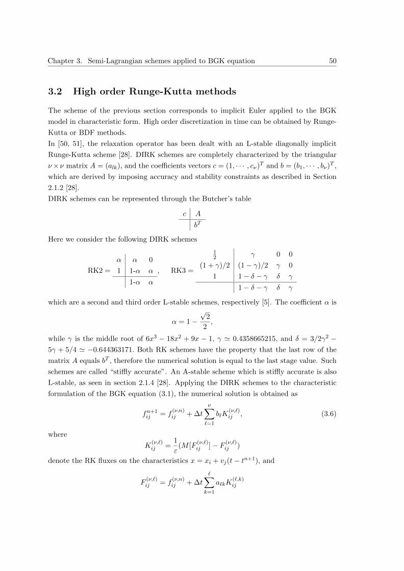
Chapter 3. Semi-Lagrangian schemes applied to BGK equation 50
3.2 High order Runge-Kutta methods
The scheme of the previous section corresponds to implicit Euler applied to the BGK
model in characteristic form. High order discretization in time can be obtained by Runge-
Kutta or BDF methods.
In [50, 51], the relaxation operator has been dealt with an L-stable diagonally implicit
Runge-Kutta scheme [28]. DIRK schemes are completely characterized by the triangular
ν×ν matrix A = (alk), and the coefficients vectors c = (1, · · · , cν)T and b = (b1, · · · , bν)T ,
which are derived by imposing accuracy and stability constraints as described in Section
2.1.2 [28].
DIRK schemes can be represented through the Butcher’s table
c A
bT
Here we consider the following DIRK schemes
RK2 =
α α 0
1 1-α α
1-α α
, RK3 =
12 γ 0 0
(1 + γ)/2 (1− γ)/2 γ 0
1 1− δ − γ δ γ
1− δ − γ δ γ
which are a second and third order L-stable schemes, respectively [5]. The coefficient α is
α = 1−√
2
2,
while γ is the middle root of 6x3 − 18x2 + 9x − 1, γ ' 0.4358665215, and δ = 3/2γ2 −5γ + 5/4 ' −0.644363171. Both RK schemes have the property that the last row of the
matrix A equals bT , therefore the numerical solution is equal to the last stage value. Such
schemes are called “stiffly accurate”. An A-stable scheme which is stiffly accurate is also
L-stable, as seen in section 2.1.4 [28]. Applying the DIRK schemes to the characteristic
formulation of the BGK equation (3.1), the numerical solution is obtained as
fn+1ij = f
(ν,n)ij + ∆t
ν∑
`=1
b`K(ν,`)ij , (3.6)
where
K(ν,`)ij =
1
ε(M [F
(ν,`)ij ]− F (ν,`)
ij )
denote the RK fluxes on the characteristics x = xi + vj(t− tn+1), and
F(ν,`)ij = f
(ν,n)ij + ∆t
∑
k=1
a`kK(`,k)ij
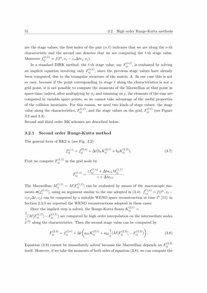
51 3.2. High order Runge-Kutta methods
are the stage values; the first index of the pair (ν, `) indicates that we are along the ν-th
characteristic and the second one denotes that we are computing the `-th stage value.
Moreover f(ν,n)ij ≡ f(tn, xi − cν∆tvj , vj).
In a standard DIRK method, the `-th stage value, say F(ν,`)ij , is evaluated by solving
an implicit equation involving only F(ν,`)ij , since the previous stage values have already
been computed, due to the triangular structure of the matrix A. In our case this is not
so easy, because if the point corresponding to stage ` along the characteristics is not a
grid point, it is not possible to compute the moments of the Maxwellian at that point in
space-time; indeed, after multiplying by φj and summing on j, the elements of the sum are
computed in variable space points, so we cannot take advantage of the useful properties
of the collision invariants. For this reason, we need two kinds of stage values: the stage
value along the characteristics, F(ν,`)ij , and the stage values on the grid, F
(`,`)ij (see Figure
3.2 and 3.3).
Second and third order RK schemes are described below.
3.2.1 Second order Runge-Kutta method
The general form of RK2 is (see Fig. 3.2)
fn+1ij = f
(2,n)ij + ∆t(b1K
(2,1)ij + b2K
(2,2)ij ). (3.7)
First we compute F(1,1)ij in the grid node by
F(1,1)ij =
εf(1,n)ij + ∆ta11M
(1,1)ij
ε+ ∆ta11.
The Maxwellian M(1,1)ij = M [F
(1,1)ij ] can be evaluated by means of the macroscopic mo-
ments m[f(1,n)i· ], using an argument similar to the one adopted in (3.4). f
(1,n)i,j = f(tn, xi−
c1vj∆t, vj) can be computed by a suitable WENO space reconstruction at time tn [11]; in
Section 2.3.3 we reported the WENO reconstructions adopted in these cases.
Once the implicit step is solved, the Runge-Kutta fluxes K(2,1)ij =
1
ε(M [F
(1,1)ij ]−F (1,1)
ij ) are computed by high order interpolation on the intermediate nodes
x(3) along the characteristics. Then the second stage value can be computed by
F(2,2)ij = f
(2,n)ij + ∆t
(a21K
(2,1)ij + a22
1
ε(M [F
(2,2)ij ]− F (2,2)
ij )
). (3.8)
Equation (3.8) cannot be immediately solved because the Maxwellian depends on F(2,2)ij
itself. However, if we take the moments of both sides of equation (3.8), we can compute the
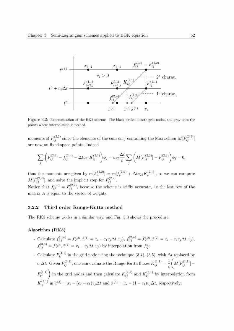
Chapter 3. Semi-Lagrangian schemes applied to BGK equation 52
x(1)x(2) x(3)
xi−2 xi−1
xi
tn
tn + c1∆t
tn+1fn+1ij ≡ F
(2,2)ij
F(1,1)ijF
(1,1)i−1,jF
(1,1)i−2,j
K(2,1)i,j
vj > 0
f(1,n)ijf
(2,n)ij
2 charac.
1 charac.
Figure 3.2: Representation of the RK2 scheme. The black circles denote grid nodes, the gray ones the
points where interpolation is needed.
moments of F(2,2)ij since the elements of the sum on j containing the Maxwellian M [F
(2,2)ij ]
are now on fixed space points. Indeed
∑
j
(F
(2,2)ij − f (2,n)
ij −∆ta21K(2,1)ij
)φj = a22
∆t
ε
∑
j
(M [F
(2,2)ij ]− F (2,2)
ij
)φj = 0,
thus the moments are given by m[F(2,2)i· ] = m[f
(2,n)i· + ∆ta21K
(2,1)i· ], so we can compute
M [F(2,2)ij ], and solve the implicit step for F
(2,2)ij .
Notice that fn+1ij = F
(2,2)ij , because the scheme is stiffly accurate, i.e the last row of the
matrix A is equal to the vector of weights.
3.2.2 Third order Runge-Kutta method
The RK3 scheme works in a similar way, and Fig. 3.3 shows the procedure.
Algorithm (RK3)
- Calculate f(1,n)i,j = f(tn, x(1) = xi − c1vj∆t, vj), f
(2,n)i,j = f(tn, x(2) = xi − c2vj∆t, vj),
f(3,n)i,j = f(tn, x(4) = xi − vj∆t, vj) by interpolation from fn·j ;
- Calculate F(1,1)ij in the grid node using the technique (3.4), (3.5), with ∆t replaced by
c1∆t. Given F(1,1)ij , one can evaluate the Runge-Kutta fluxes K
(1,1)ij =
1
ε
(M [F
(1,1)ij ]−
F(1,1)ij
)in the grid nodes and then calculate K
(2,1)ij and K
(3,1)ij by interpolation from
K(1,1)·j in x(3) = xi − (c2 − c1)vj∆t and x(5) = xi − (1− c1)vj∆t, respectively;
53 3.3. BDF methods
- Calculate F(2,2)ij in the grid node using RK2 scheme described in the previous section
with time step c2∆t. Given F(2,2)ij , one can evaluate K
(2,2)ij =
1
ε
(M [F
(2,2)ij ]− F (2,2)
ij
)
in the grid nodes and then calculate K(3,2)ij by interpolation from K
(2,2)·j in x(6) =
xi − (1− c2)vj∆t;
- Now one can update fn+1ij using (3.6), taking into account that the method is stiffly
accurate and using the properties of the collision invariants to solve the implicit step.
Summary of the Runge-Kutta schemes
Three schemes based on RK are tested:
- scheme RK2W23: uses WENO23 for the interpolation and RK2, as described above,
for time integration;
- scheme RK3W23: uses WENO23 for the interpolation and RK3, as described above,
for time integration;
- scheme RK3W35: uses WENO35 for interpolation and RK3 for time integration.
Remark.
In practice, the Runge-Kutta fluxes can be computed from the internal stages. For exam-
ple, using RK2, we have
K(1,1)ij =
1
ε(M [F
(1,1)ij ]− F (1,1)
ij ) =F
(1,1)ij − f (1,n)
ij
∆ta11.
The latter expression can be used in the limit ε→ 0, with no constraint on the time step.
3.3 BDF methods
In this section we present a new family of high order semi-Lagrangian schemes, based
on BDF. The backward differentiation formulas are implicit linear multistep methods for
the numerical integration of ordinary differential equations y′ = g(t, y), and they had
been recalled in Section 2.2.2. Using the linear polynomial interpolating yn and yn−1 one
obtains the simplest first order BDF method (BDF1) that corresponds to backward Euler,
used in Section 3.1.
Here the characteristic formulation of the BGK model, that leads to ordinary differ-
ential equations, is approximated by using BDF2 and BDF3 methods, in order to obtain
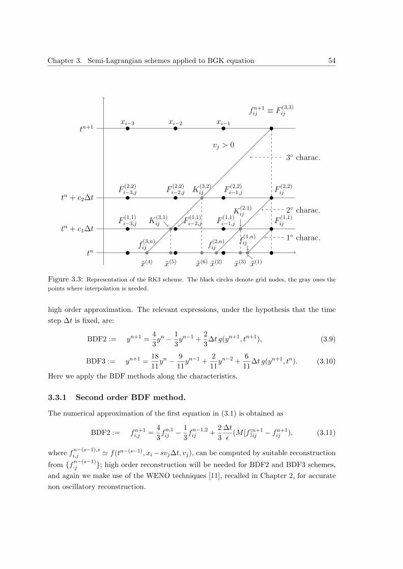
Chapter 3. Semi-Lagrangian schemes applied to BGK equation 54
xi−3 xi−2 xi−1
x(1)x(2) x(3)x(4) x(5) x(6)
tn
tn + c1∆t
tn + c2∆t
tn+1
fn+1ij ≡ F
(3,3)ij
K(3,2)ijF
(2,2)i−3,j F
(2,2)i−2,j F
(2,2)i−1,j F
(2,2)ij
F(1,1)i−3,j F
(1,1)i−2,j F
(1,1)i−1,j F
(1,1)ijK
(3,1)ij
f(3,n)ij
vj > 0
f(1,n)ijf
(2,n)ij
K(2,1)ij
3 charac.
2 charac.
1 charac.
Figure 3.3: Representation of the RK3 scheme. The black circles denote grid nodes, the gray ones the
points where interpolation is needed.
high order approximation. The relevant expressions, under the hypothesis that the time
step ∆t is fixed, are:
BDF2 := yn+1 =4
3yn − 1
3yn−1 +
2
3∆t g(yn+1, tn+1), (3.9)
BDF3 := yn+1 =18
11yn − 9
11yn−1 +
2
11yn−2 +
6
11∆t g(yn+1, tn). (3.10)
Here we apply the BDF methods along the characteristics.
3.3.1 Second order BDF method.
The numerical approximation of the first equation in (3.1) is obtained as
BDF2 := fn+1i,j =
4
3fn,1ij −
1
3fn−1,2ij +
2
3
∆t
ε(M [f ]n+1
ij − fn+1ij ), (3.11)
where fn−(s−1),si,j ' f(tn−(s−1), xi−svj∆t, vj), can be computed by suitable reconstruction
from fn−(s−1)·j ; high order reconstruction will be needed for BDF2 and BDF3 schemes,
and again we make use of the WENO techniques [11], recalled in Chapter 2, for accurate
non oscillatory reconstruction.
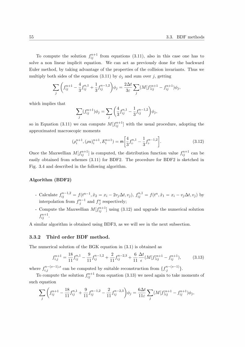
55 3.3. BDF methods
To compute the solution fn+1ij from equations (3.11), also in this case one has to
solve a non linear implicit equation. We can act as previously done for the backward
Euler method, by taking advantage of the properties of the collision invariants. Thus we
multiply both sides of the equation (3.11) by φj and sum over j, getting
∑
j
(fn+1ij − 4
3fn,1ij +
1
3fn−1,2ij
)φj =
2∆t
3ε
∑
j
(M [f ]n+1ij − fn+1
ij )φj ,
which implies that∑
j
(fn+1ij )φj =
∑
j
(4
3fn,1ij −
1
3fn−1,2ij
)φj ,
so in Equation (3.11) we can compute M [fn+1ij ] with the usual procedure, adopting the
approximated macroscopic moments
(ρn+1i , (ρu)n+1
i , En+1i ) = m
[4
3fn,1i· −
1
3fn−1,2i·
]. (3.12)
Once the Maxwellian M [fn+1ij ] is computed, the distribution function value fn+1
ij can be
easily obtained from schemes (3.11) for BDF2. The procedure for BDF2 is sketched in
Fig. 3.4 and described in the following algorithm.
Algorithm (BDF2)
- Calculate fn−1,2ij = f(tn−1, x2 = xi − 2vj∆t, vj), f
n,1ij = f(tn, x1 = xi − vj∆t, vj) by
interpolation from fn−1·j and fn·j respectively;
- Compute the Maxwellian M [fn+1ij ] using (3.12) and upgrade the numerical solution
fn+1ij .
A similar algorithm is obtained using BDF3, as we will see in the next subsection.
3.3.2 Third order BDF method.
The numerical solution of the BGK equation in (3.1) is obtained as
fn+1i,j =
18
11fn,1ij −
9
11fn−1,2ij +
2
11fn−2,3ij +
6
11
∆t
ε(M [f ]n+1
ij − fn+1ij ), (3.13)
where fn−(s−1),si,j can be computed by suitable reconstruction from fn−(s−1)
·j .To compute the solution fn+1
ij from equation (3.13) we need again to take moments of
such equation
∑
j
(fn+1ij − 18
11fn,1ij +
9
11fn−1,2ij − 2
11fn−2,3ij
)φj =
6∆t
11ε
∑
j
(M [f ]n+1ij − fn+1
ij )φj ,
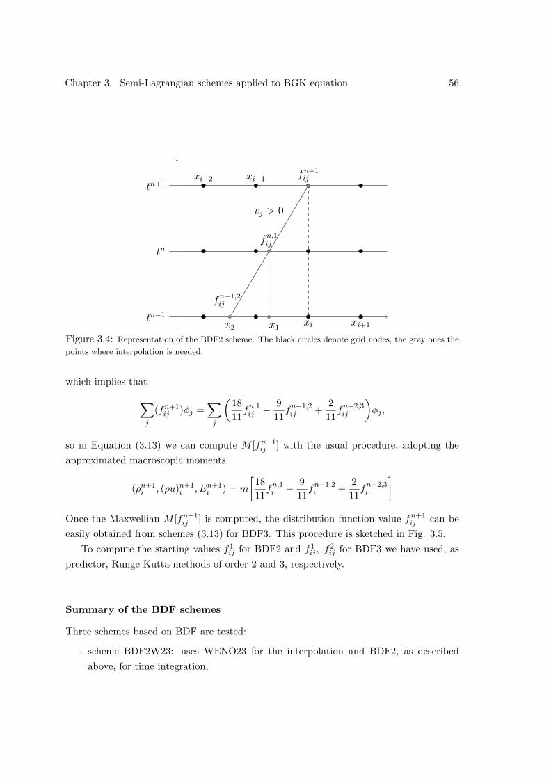
Chapter 3. Semi-Lagrangian schemes applied to BGK equation 56
xi−2 xi−1
xi xi+1tn−1
tn
tn+1fn+1ij
vj > 0
fn−1,2ij
fn,1ij
x2 x1
Figure 3.4: Representation of the BDF2 scheme. The black circles denote grid nodes, the gray ones the
points where interpolation is needed.
which implies that
∑
j
(fn+1ij )φj =
∑
j
(18
11fn,1ij −
9
11fn−1,2ij +
2
11fn−2,3ij
)φj ,
so in Equation (3.13) we can compute M [fn+1ij ] with the usual procedure, adopting the
approximated macroscopic moments
(ρn+1i , (ρu)n+1
i , En+1i ) = m
[18
11fn,1i· −
9
11fn−1,2i· +
2
11fn−2,3i·
]
Once the Maxwellian M [fn+1ij ] is computed, the distribution function value fn+1
ij can be
easily obtained from schemes (3.13) for BDF3. This procedure is sketched in Fig. 3.5.
To compute the starting values f1ij for BDF2 and f1
ij , f2ij for BDF3 we have used, as
predictor, Runge-Kutta methods of order 2 and 3, respectively.
Summary of the BDF schemes
Three schemes based on BDF are tested:
- scheme BDF2W23: uses WENO23 for the interpolation and BDF2, as described
above, for time integration;
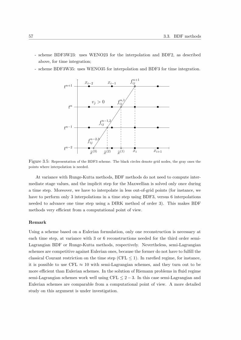
57 3.3. BDF methods
- scheme BDF3W23: uses WENO23 for the interpolation and BDF2, as described
above, for time integration;
- scheme BDF3W35: uses WENO35 for interpolation and BDF3 for time integration.
xi−2 xi−1
xi xi+1tn−2
tn−1
tn
tn+1fn+1ij
vj > 0
fn−2,3ij
fn,1ij
fn−1,2ij
x(3) x(2) x(1)
Figure 3.5: Representation of the BDF3 scheme. The black circles denote grid nodes, the gray ones the
points where interpolation is needed.
At variance with Runge-Kutta methods, BDF methods do not need to compute inter-
mediate stage values, and the implicit step for the Maxwellian is solved only once during
a time step. Moreover, we have to interpolate in less out-of-grid points (for instance, we
have to perform only 3 interpolations in a time step using BDF3, versus 6 interpolations
needed to advance one time step using a DIRK method of order 3). This makes BDF
methods very efficient from a computational point of view.
Remark
Using a scheme based on a Eulerian formulation, only one reconstruction is necessary at
each time step, at variance with 3 or 6 reconstructions needed for the third order semi-
Lagrangian BDF or Runge-Kutta methods, respectively. Nevertheless, semi-Lagrangian
schemes are competitive against Eulerian ones, because the former do not have to fulfill the
classical Courant restriction on the time step (CFL ≤ 1). In rarefied regime, for instance,
it is possible to use CFL ≈ 10 with semi-Lagrangian schemes, and they turn out to be
more efficient than Eulerian schemes. In the solution of Riemann problems in fluid regime
semi-Lagrangian schemes work well using CFL ≤ 2− 3. In this case semi-Lagrangian and
Eulerian schemes are comparable from a computational point of view. A more detailed
study on this argument is under investigation.
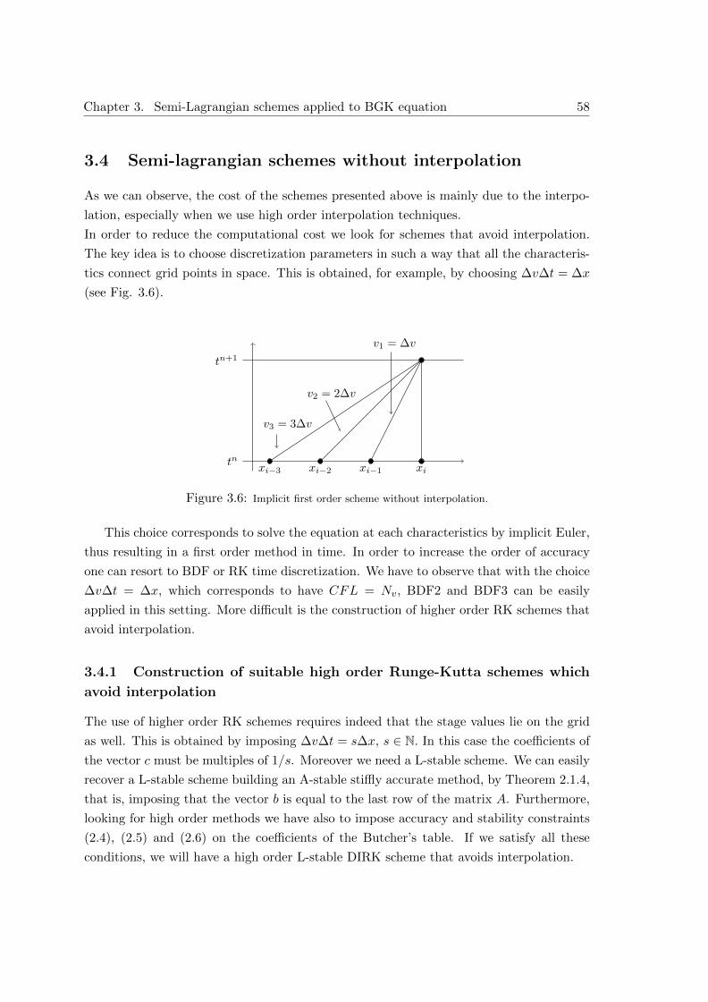
Chapter 3. Semi-Lagrangian schemes applied to BGK equation 58
3.4 Semi-lagrangian schemes without interpolation
As we can observe, the cost of the schemes presented above is mainly due to the interpo-
lation, especially when we use high order interpolation techniques.
In order to reduce the computational cost we look for schemes that avoid interpolation.
The key idea is to choose discretization parameters in such a way that all the characteris-
tics connect grid points in space. This is obtained, for example, by choosing ∆v∆t = ∆x
(see Fig. 3.6).
xi−2 xi−1 xitn
tn+1
v1 = ∆v
v2 = 2∆v
v3 = 3∆v
xi−3
Figure 3.6: Implicit first order scheme without interpolation.
This choice corresponds to solve the equation at each characteristics by implicit Euler,
thus resulting in a first order method in time. In order to increase the order of accuracy
one can resort to BDF or RK time discretization. We have to observe that with the choice
∆v∆t = ∆x, which corresponds to have CFL = Nv, BDF2 and BDF3 can be easily
applied in this setting. More difficult is the construction of higher order RK schemes that
avoid interpolation.
3.4.1 Construction of suitable high order Runge-Kutta schemes which
avoid interpolation
The use of higher order RK schemes requires indeed that the stage values lie on the grid
as well. This is obtained by imposing ∆v∆t = s∆x, s ∈ N. In this case the coefficients of
the vector c must be multiples of 1/s. Moreover we need a L-stable scheme. We can easily
recover a L-stable scheme building an A-stable stiffly accurate method, by Theorem 2.1.4,
that is, imposing that the vector b is equal to the last row of the matrix A. Furthermore,
looking for high order methods we have also to impose accuracy and stability constraints
(2.4), (2.5) and (2.6) on the coefficients of the Butcher’s table. If we satisfy all these
conditions, we will have a high order L-stable DIRK scheme that avoids interpolation.
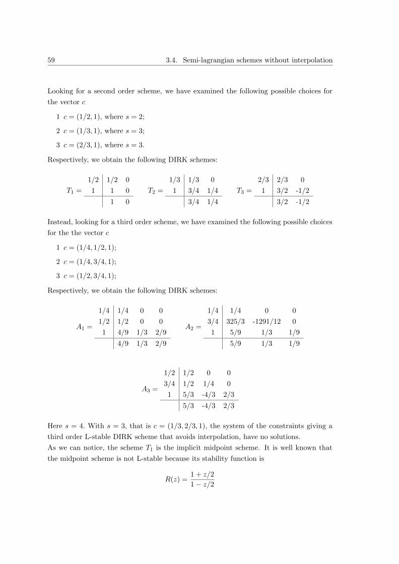
59 3.4. Semi-lagrangian schemes without interpolation
Looking for a second order scheme, we have examined the following possible choices for
the vector c
1 c = (1/2, 1), where s = 2;
2 c = (1/3, 1), where s = 3;
3 c = (2/3, 1), where s = 3.
Respectively, we obtain the following DIRK schemes:
T1 =
1/2 1/2 0
1 1 0
1 0
T2 =
1/3 1/3 0
1 3/4 1/4
3/4 1/4
T3 =
2/3 2/3 0
1 3/2 -1/2
3/2 -1/2
Instead, looking for a third order scheme, we have examined the following possible choices
for the the vector c
1 c = (1/4, 1/2, 1);
2 c = (1/4, 3/4, 1);
3 c = (1/2, 3/4, 1);
Respectively, we obtain the following DIRK schemes:
A1 =
1/4 1/4 0 0
1/2 1/2 0 0
1 4/9 1/3 2/9
4/9 1/3 2/9
A2 =
1/4 1/4 0 0
3/4 325/3 -1291/12 0
1 5/9 1/3 1/9
5/9 1/3 1/9
A3 =
1/2 1/2 0 0
3/4 1/2 1/4 0
1 5/3 -4/3 2/3
5/3 -4/3 2/3
Here s = 4. With s = 3, that is c = (1/3, 2/3, 1), the system of the constraints giving a
third order L-stable DIRK scheme that avoids interpolation, have no solutions.
As we can notice, the scheme T1 is the implicit midpoint scheme. It is well known that
the midpoint scheme is not L-stable because its stability function is
R(z) =1 + z/2
1− z/2
Chapter 3. Semi-Lagrangian schemes applied to BGK equation 60
that does not fulfill Definition 2.6 as z → ∞. The others schemes, T2, T3, A1, A2, A3
are stiffly accurate by construction. By Theorem 2.1.4, if they are A-stable, they will
be L-stable. In Fig. 3.7 the stability regions of such schemes are shown. Recalling that
a Runge-Kutta scheme is A-stable if the A-stability region includes C−, by Fig. 3.7 we
can deduce that only the schemes T2 and A3 are A-stable and therefore they are L-stable
DIRK schemes avoiding interpolation of second and third order, respectively.
Using schemes that avoid the interpolation, the choice of the time step is determined by
the other discretization steps, and the CFL number is fixed to sNv for DIRK schemes,
whereas is Nv for each BDF methods. This means that we have very large time step for
DIRK schemes. The semi-Lagrangian nature of the family of schemes introduced in the
previous sections, allows us to use large CFL numbers. Nonetheless, for example, choosing
Nv = 20, the use of schemes with s = 4 leads to CFL = 80. In these cases, i.e. scheme A3,
some instabilities arise in the numerical solution, but using a fine space grid we are able to
obtain good numerical solution. The high number of space points is not a computational
problem, because these schemes does not require interpolation and for this reason are very
efficient from a computational point of view. We notice that the BDF schemes do have
not this problem because in this case s = 1. Moreover these schemes are very simple to
implement and therefore each time step can be advanced very efficiently.
A comparison with more standard semi-Lagrangian methods that make use of interpolation
will be presented in the Section 3.6 on numerical results. Numerical experiments show
that schemes without interpolation can be cost-effective, especially for problems that do
not require a fine mesh in velocity. In particular, BDF3 without interpolation appears to
have the best performance in most tests.
3.5 Chu reduction model
The schemes presented before have been extended to treat problems in 3D in velocity,
1D in space, in slab geometry. The starting point is the Chu reduction [15] introduced
in Section 1.4, which, under suitable symmetry assumption, allows to transform a 3D
equation (in velocity) in a system of two equations 1D (in velocity), to which the schemes
previously introduced can be applied.
The system of BGK equations to discretize is the following:
∂gi∂t
+ v∂gi∂x
=1
ε(M [f ]i − gi), (t, x, v) ∈ R+ × R× R, (3.14)
gs(0, x, v) = gs,0(x, v), s = 1, 2.
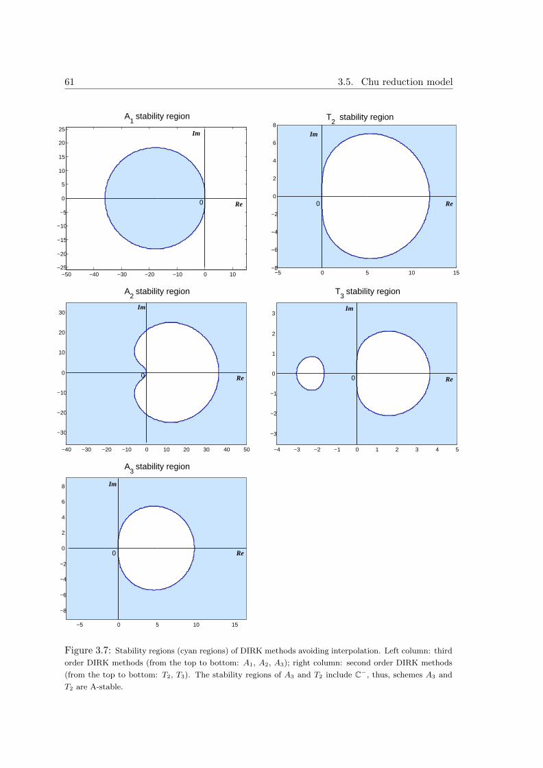
61 3.5. Chu reduction model
A1 stability region
−50 −40 −30 −20 −10 0 10−25
−20
−15
−10
−5
0
5
10
15
20
25
Re0
Im
−5 0 5 10 15−8
−6
−4
−2
0
2
4
6
8T
2 stability region
Im
Re0
−40 −30 −20 −10 0 10 20 30 40 50
−30
−20
−10
0
10
20
30
A2 stability region
Re0
Im
−4 −3 −2 −1 0 1 2 3 4 5
−3
−2
−1
0
1
2
3
T3 stability region
Re
Im
0
−5 0 5 10 15
−8
−6
−4
−2
0
2
4
6
8
A3 stability region
Re
Im
0
Figure 3.7: Stability regions (cyan regions) of DIRK methods avoiding interpolation. Left column: third
order DIRK methods (from the top to bottom: A1, A2, A3); right column: second order DIRK methods
(from the top to bottom: T2, T3). The stability regions of A3 and T2 include C−, thus, schemes A3 and
T2 are A-stable.
Chapter 3. Semi-Lagrangian schemes applied to BGK equation 62
The discrete version of the first order implicit scheme of (3.14) is
gn+1s,ij = gns,ij +
∆t
ε(Mn+1
s,ij − gn+1s,ij ) s = 1, 2. (3.15)
To solve the implicit step we have to compute m[gn+11,i· ]. The density ρn+1
i and the momen-
tum (ρu)n+1i can be easily computed multiplying the first equation of (3.15) by 1 and vj
and summing over j. In this way we get
ρn+1i = ∆v
∑
j
gn1,ij , (ρu)n+1i = ∆v
∑
j
vj gn1,ij .
To obtain the temperature Tn+1i , instead, we have to multiply by (vj − uj)
2 and by 1
respectively the first and the second equation of (3.15), and than summing over j.
Now, using the discrete analogue of (1.28):
∆v∑
j
(vj − uj)2(Mn+11,ij − gn+1
1,ij ) + ∆v∑
j
(Mn+12,ij − gn+1
2,ij ) = 0,
one can compute the temperature Tn+1i in this way:
3Rρn+1i Tn+1
i = ∆v∑
j
(vj − uj)2gn1,ij + ∆v∑
j
gn2,ij .
Once the new moments ρn+1i , (ρu)n+1
i and Tn+1i are computed, we can solve the implicit
step and upgrade the numerical solution.
In a very simple and similar way is possible to extend the high order numerical schemes
introduced before.
3.6 Numerical tests
We have considered two types of numerical tests with the purpose of verifying the accuracy
(test 1) and the shock capturing properties (test 2) of the schemes. Different values of
the Knudsen number, represented by the relaxation parameter ε, have been investigated
in order to observe the behavior of the methods varying from the rarefied (ε ' 1) to the
fluid (ε ' 10−6) regime. We use units for temperature such that R = 1.
In the first part of the section we consider the 1D model and we explore the choice
of the optimal CFL. A comparison between semi-Lagrangian schemes with and without
interpolation is also presented. The second part of the section is devoted to the results
obtained by the method applied to the 1D space–3D velocity case in slab geometry (Chu
reduction).
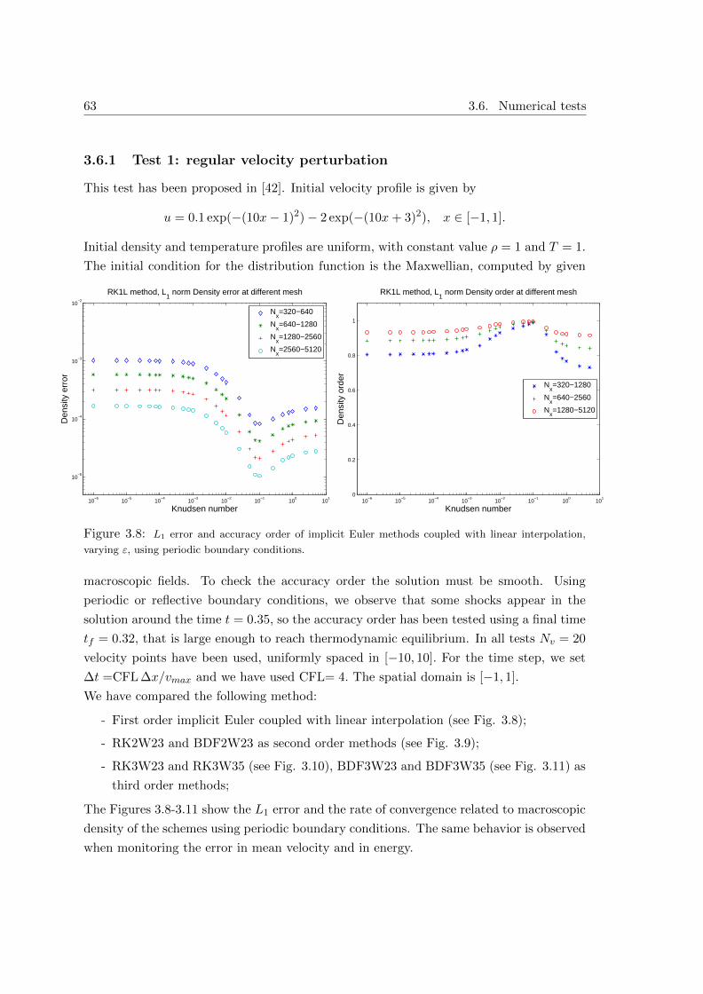
63 3.6. Numerical tests
3.6.1 Test 1: regular velocity perturbation
This test has been proposed in [42]. Initial velocity profile is given by
u = 0.1 exp(−(10x− 1)2)− 2 exp(−(10x+ 3)2), x ∈ [−1, 1].
Initial density and temperature profiles are uniform, with constant value ρ = 1 and T = 1.
The initial condition for the distribution function is the Maxwellian, computed by given
10−6
10−5
10−4
10−3
10−2
10−1
100
101
10−5
10−4
10−3
10−2
RK1L method, L1 norm Density error at different mesh
Knudsen number
Den
sity
err
or
Nx=320−640
Nx=640−1280
Nx=1280−2560
Nx=2560−5120
10−6
10−5
10−4
10−3
10−2
10−1
100
101
0
0.2
0.4
0.6
0.8
1
RK1L method, L1 norm Density order at different mesh
Knudsen number
Den
sity
ord
er
Nx=320−1280
Nx=640−2560
Nx=1280−5120
Figure 3.8: L1 error and accuracy order of implicit Euler methods coupled with linear interpolation,
varying ε, using periodic boundary conditions.
macroscopic fields. To check the accuracy order the solution must be smooth. Using
periodic or reflective boundary conditions, we observe that some shocks appear in the
solution around the time t = 0.35, so the accuracy order has been tested using a final time
tf = 0.32, that is large enough to reach thermodynamic equilibrium. In all tests Nv = 20
velocity points have been used, uniformly spaced in [−10, 10]. For the time step, we set
∆t =CFL ∆x/vmax and we have used CFL= 4. The spatial domain is [−1, 1].
We have compared the following method:
- First order implicit Euler coupled with linear interpolation (see Fig. 3.8);
- RK2W23 and BDF2W23 as second order methods (see Fig. 3.9);
- RK3W23 and RK3W35 (see Fig. 3.10), BDF3W23 and BDF3W35 (see Fig. 3.11) as
third order methods;
The Figures 3.8-3.11 show the L1 error and the rate of convergence related to macroscopic
density of the schemes using periodic boundary conditions. The same behavior is observed
when monitoring the error in mean velocity and in energy.
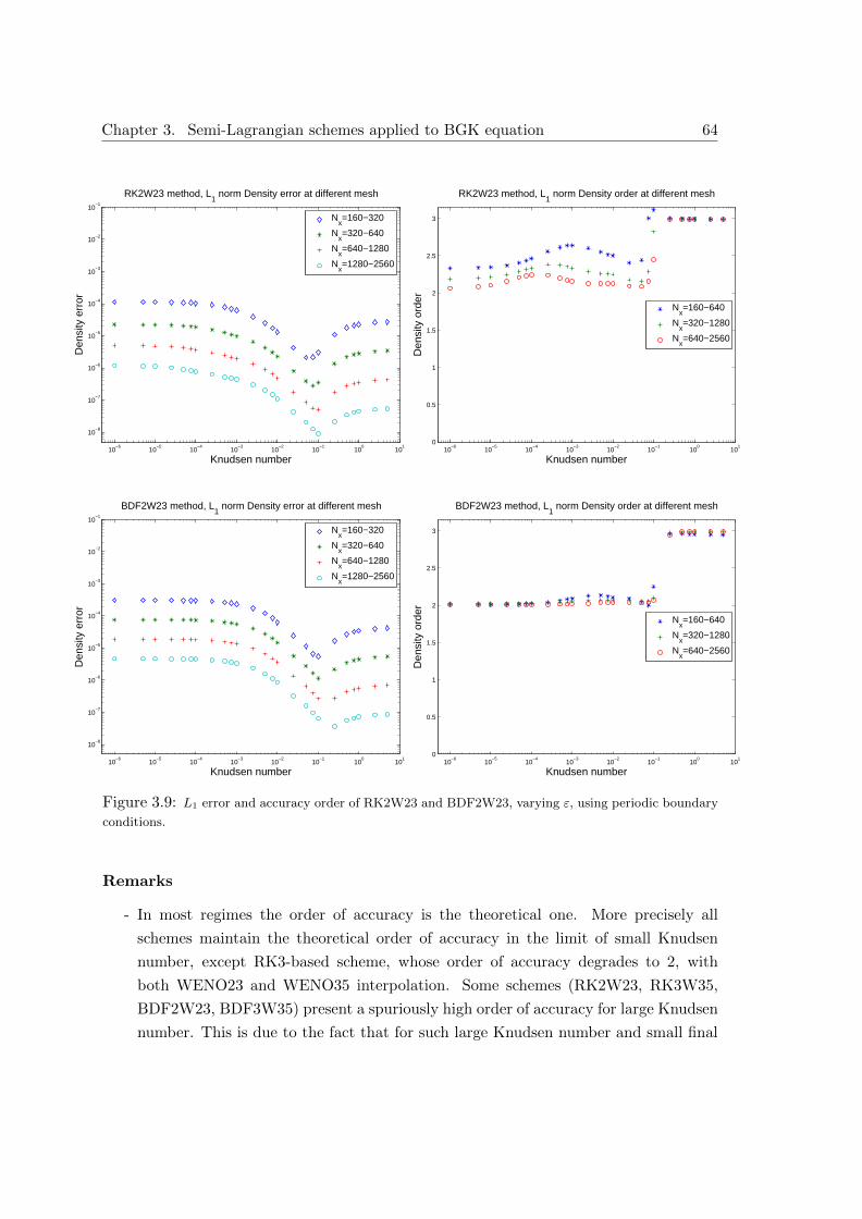
Chapter 3. Semi-Lagrangian schemes applied to BGK equation 64
10−6
10−5
10−4
10−3
10−2
10−1
100
101
10−8
10−7
10−6
10−5
10−4
10−3
10−2
10−1
RK2W23 method, L1 norm Density error at different mesh
Knudsen number
Den
sity
err
or
Nx=160−320
Nx=320−640
Nx=640−1280
Nx=1280−2560
10−6
10−5
10−4
10−3
10−2
10−1
100
101
0
0.5
1
1.5
2
2.5
3
RK2W23 method, L1 norm Density order at different mesh
Knudsen number
Den
sity
ord
er
Nx=160−640
Nx=320−1280
Nx=640−2560
10−6
10−5
10−4
10−3
10−2
10−1
100
101
10−8
10−7
10−6
10−5
10−4
10−3
10−2
10−1
BDF2W23 method, L1 norm Density error at different mesh
Knudsen number
Den
sity
err
or
Nx=160−320
Nx=320−640
Nx=640−1280
Nx=1280−2560
10−6
10−5
10−4
10−3
10−2
10−1
100
101
0
0.5
1
1.5
2
2.5
3
BDF2W23 method, L1 norm Density order at different mesh
Knudsen number
Den
sity
ord
er
Nx=160−640
Nx=320−1280
Nx=640−2560
Figure 3.9: L1 error and accuracy order of RK2W23 and BDF2W23, varying ε, using periodic boundary
conditions.
Remarks
- In most regimes the order of accuracy is the theoretical one. More precisely all
schemes maintain the theoretical order of accuracy in the limit of small Knudsen
number, except RK3-based scheme, whose order of accuracy degrades to 2, with
both WENO23 and WENO35 interpolation. Some schemes (RK2W23, RK3W35,
BDF2W23, BDF3W35) present a spuriously high order of accuracy for large Knudsen
number. This is due to the fact that for such large Knudsen number and small final
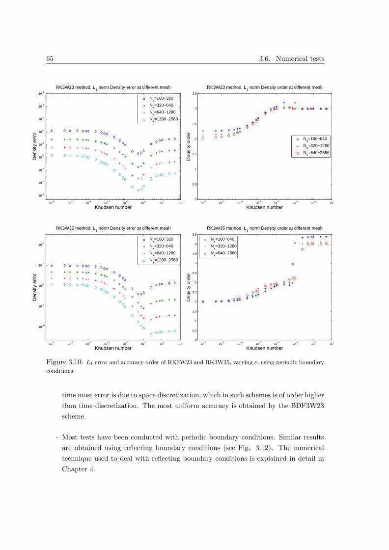
65 3.6. Numerical tests
10−6
10−5
10−4
10−3
10−2
10−1
100
101
10−9
10−8
10−7
10−6
10−5
10−4
10−3
10−2
10−1
RK3W23 method, L1 norm Density error at different mesh
Knudsen number
Den
sity
err
or
Nx=160−320
Nx=320−640
Nx=640−1280
Nx=1280−2560
10−6
10−5
10−4
10−3
10−2
10−1
100
101
0
0.5
1
1.5
2
2.5
3
3.5
RK3W23 method, L1 norm Density order at different mesh
Knudsen number
Den
sity
ord
er
Nx=160−640
Nx=320−1280
Nx=640−2560
10−6
10−5
10−4
10−3
10−2
10−1
100
101
10−10
10−8
10−6
10−4
10−2
RK3W35 method, L1 norm Density error at different mesh
Knudsen number
Den
sity
err
or
Nx=160−320
Nx=320−640
Nx=640−1280
Nx=1280−2560
10−6
10−5
10−4
10−3
10−2
10−1
100
101
0
0.5
1
1.5
2
2.5
3
3.5
4
4.5
5
5.5
RK3W35 method, L1 norm Density order at different mesh
Knudsen number
Den
sity
ord
er
Nx=160−640
Nx=320−1280
Nx=640−2560
Figure 3.10: L1 error and accuracy order of RK3W23 and RK3W35, varying ε, using periodic boundary
conditions.
time most error is due to space discretization, which in such schemes is of order higher
than time discretization. The most uniform accuracy is obtained by the BDF3W23
scheme.
- Most tests have been conducted with periodic boundary conditions. Similar results
are obtained using reflecting boundary conditions (see Fig. 3.12). The numerical
technique used to deal with reflecting boundary conditions is explained in detail in
Chapter 4.
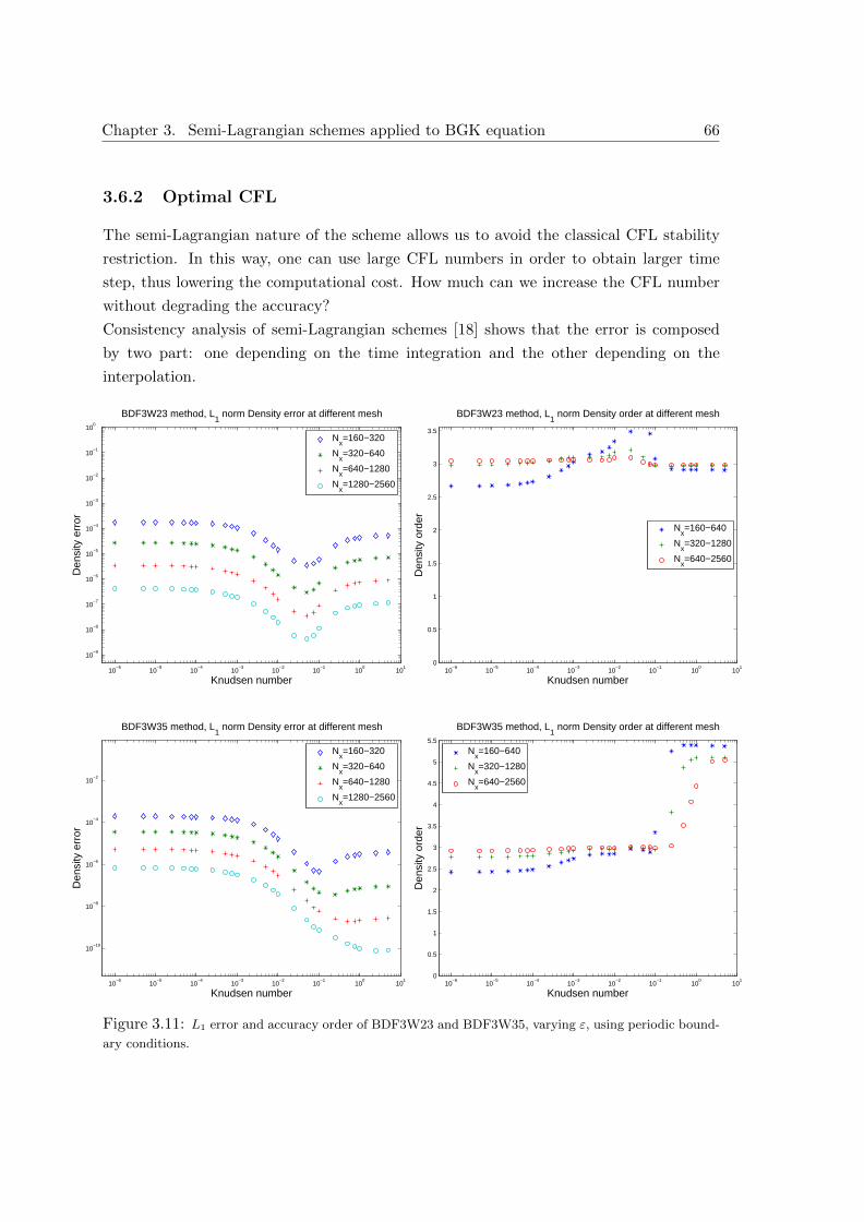
Chapter 3. Semi-Lagrangian schemes applied to BGK equation 66
3.6.2 Optimal CFL
The semi-Lagrangian nature of the scheme allows us to avoid the classical CFL stability
restriction. In this way, one can use large CFL numbers in order to obtain larger time
step, thus lowering the computational cost. How much can we increase the CFL number
without degrading the accuracy?
Consistency analysis of semi-Lagrangian schemes [18] shows that the error is composed
by two part: one depending on the time integration and the other depending on the
interpolation.
10−6
10−5
10−4
10−3
10−2
10−1
100
101
10−9
10−8
10−7
10−6
10−5
10−4
10−3
10−2
10−1
100
BDF3W23 method, L1 norm Density error at different mesh
Knudsen number
Den
sity
err
or
Nx=160−320
Nx=320−640
Nx=640−1280
Nx=1280−2560
10−6
10−5
10−4
10−3
10−2
10−1
100
101
0
0.5
1
1.5
2
2.5
3
3.5
BDF3W23 method, L1 norm Density order at different mesh
Knudsen number
Den
sity
ord
er
Nx=160−640
Nx=320−1280
Nx=640−2560
10−6
10−5
10−4
10−3
10−2
10−1
100
101
10−10
10−8
10−6
10−4
10−2
BDF3W35 method, L1 norm Density error at different mesh
Knudsen number
Den
sity
err
or
Nx=160−320
Nx=320−640
Nx=640−1280
Nx=1280−2560
10−6
10−5
10−4
10−3
10−2
10−1
100
101
0
0.5
1
1.5
2
2.5
3
3.5
4
4.5
5
5.5
BDF3W35 method, L1 norm Density order at different mesh
Knudsen number
Den
sity
ord
er
Nx=160−640
Nx=320−1280
Nx=640−2560
Figure 3.11: L1 error and accuracy order of BDF3W23 and BDF3W35, varying ε, using periodic bound-
ary conditions.
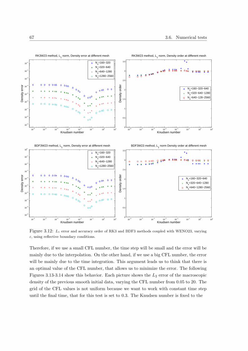
67 3.6. Numerical tests
10−6
10−5
10−4
10−3
10−2
10−1
100
101
10−9
10−8
10−7
10−6
10−5
10−4
10−3
10−2
10−1
RK3W23 method, L1 norm, Density error at different mesh
Knudsen number
Den
sity
err
or
Nx=160−320
Nx=320−640
Nx=640−1280
Nx=1280−2560
10−6
10−5
10−4
10−3
10−2
10−1
100
101
0
0.5
1
1.5
2
2.5
3
3.5
RK3W23 method, L1 norm, Density order at different mesh
Knudsen number
Den
sity
ord
er
Nx=160−320−640
Nx=320−640−1280
Nx=640−128−2560
10−6
10−5
10−4
10−3
10−2
10−1
100
101
10−9
10−8
10−7
10−6
10−5
10−4
10−3
10−2
10−1
100
BDF3W23 method, L1 norm, Density error at different mesh
Knudsen number
Den
sity
err
or
Nx=160−320
Nx=320−640
Nx=640−1280
Nx=1280−2560
10−6
10−5
10−4
10−3
10−2
10−1
100
101
0
0.5
1
1.5
2
2.5
3
3.5
BDF3W23 method, L1 norm Density order at different mesh
Knudsen number
Den
sity
ord
er
Nx=160−320−640
Nx=320−640−1280
Nx=640−1280−2560
Figure 3.12: L1 error and accuracy order of RK3 and BDF3 methods coupled with WENO23, varying
ε, using reflective boundary conditions.
Therefore, if we use a small CFL number, the time step will be small and the error will be
mainly due to the interpolation. On the other hand, if we use a big CFL number, the error
will be mainly due to the time integration. This argument leads us to think that there is
an optimal value of the CFL number, that allows us to minimize the error. The following
Figures 3.13-3.14 show this behavior. Each picture shows the L2 error of the macroscopic
density of the previous smooth initial data, varying the CFL number from 0.05 to 20. The
grid of the CFL values is not uniform because we want to work with constant time step
until the final time, that for this test is set to 0.3. The Knudsen number is fixed to the
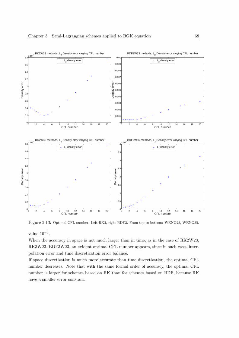
Chapter 3. Semi-Lagrangian schemes applied to BGK equation 68
0 2 4 6 8 10 12 14 16 18 200
0.2
0.4
0.6
0.8
1
1.2
1.4
1.6
1.8x 10
−3RK2W23 methods, L
2 Density error varying CFL number
CFL number
Den
sity
err
or
L2 density error
0 2 4 6 8 10 12 14 16 18 200
0.001
0.002
0.003
0.004
0.005
0.006
0.007
0.008
0.009
0.01
BDF2W23 methods, L2 Density error varying CFL number
CFL number
Den
sity
err
or
L2 density error
0 2 4 6 8 10 12 14 16 18 200
0.2
0.4
0.6
0.8
1
1.2
1.4
1.6
1.8x 10
−3RK2W35 methods, L
2 Density error varying CFL number
CFL number
Den
sity
err
or
L2 density error
0 2 4 6 8 10 12 14 16 18 200
0.5
1
1.5
2
2.5
3
3.5
4x 10
−3BDF2W35 methods, L
2 Density error varying CFL number
CFL number
Den
sity
err
or
L2 density error
Figure 3.13: Optimal CFL number. Left RK2, right BDF2. From top to bottom: WENO23, WENO35.
value 10−4.
When the accuracy in space is not much larger than in time, as in the case of RK2W23,
RK3W23, BDF3W23, an evident optimal CFL number appears, since in such cases inter-
polation error and time discretization error balance.
If space discretization is much more accurate than time discretization, the optimal CFL
number decreases. Note that with the same formal order of accuracy, the optimal CFL
number is larger for schemes based on RK than for schemes based on BDF, because RK
have a smaller error constant.
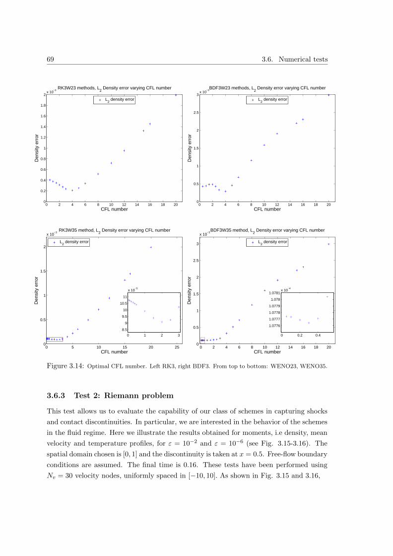
69 3.6. Numerical tests
0 2 4 6 8 10 12 14 16 18 200
0.2
0.4
0.6
0.8
1
1.2
1.4
1.6
1.8
2x 10
−3RK3W23 methods, L
2 Density error varying CFL number
CFL number
Den
sity
err
or
L2 density error
0 2 4 6 8 10 12 14 16 18 200
0.5
1
1.5
2
2.5
3x 10
−3BDF3W23 methods, L
2 Density error varying CFL number
CFL number
Den
sity
err
or
L2 density error
0 5 10 15 20 250
0.5
1
1.5
2
x 10−3
RK3W35 method, L2 Density error varying CFL number
CFL number
Den
sity
err
or
L2 density error
0 1 2 3
8.5
9
9.5
10
10.5
11
x 10−5
0 2 4 6 8 10 12 14 16 18 200
0.5
1
1.5
2
2.5
3
x 10−3
BDF3W35 method, L2 Density error varying CFL number
CFL number
Den
sity
err
or
L2 density error
0 0.2 0.4
1.0776
1.0777
1.0778
1.0779
1.078
1.0781x 10
−4
Figure 3.14: Optimal CFL number. Left RK3, right BDF3. From top to bottom: WENO23, WENO35.
3.6.3 Test 2: Riemann problem
This test allows us to evaluate the capability of our class of schemes in capturing shocks
and contact discontinuities. In particular, we are interested in the behavior of the schemes
in the fluid regime. Here we illustrate the results obtained for moments, i.e density, mean
velocity and temperature profiles, for ε = 10−2 and ε = 10−6 (see Fig. 3.15-3.16). The
spatial domain chosen is [0, 1] and the discontinuity is taken at x = 0.5. Free-flow boundary
conditions are assumed. The final time is 0.16. These tests have been performed using
Nv = 30 velocity nodes, uniformly spaced in [−10, 10]. As shown in Fig. 3.15 and 3.16,
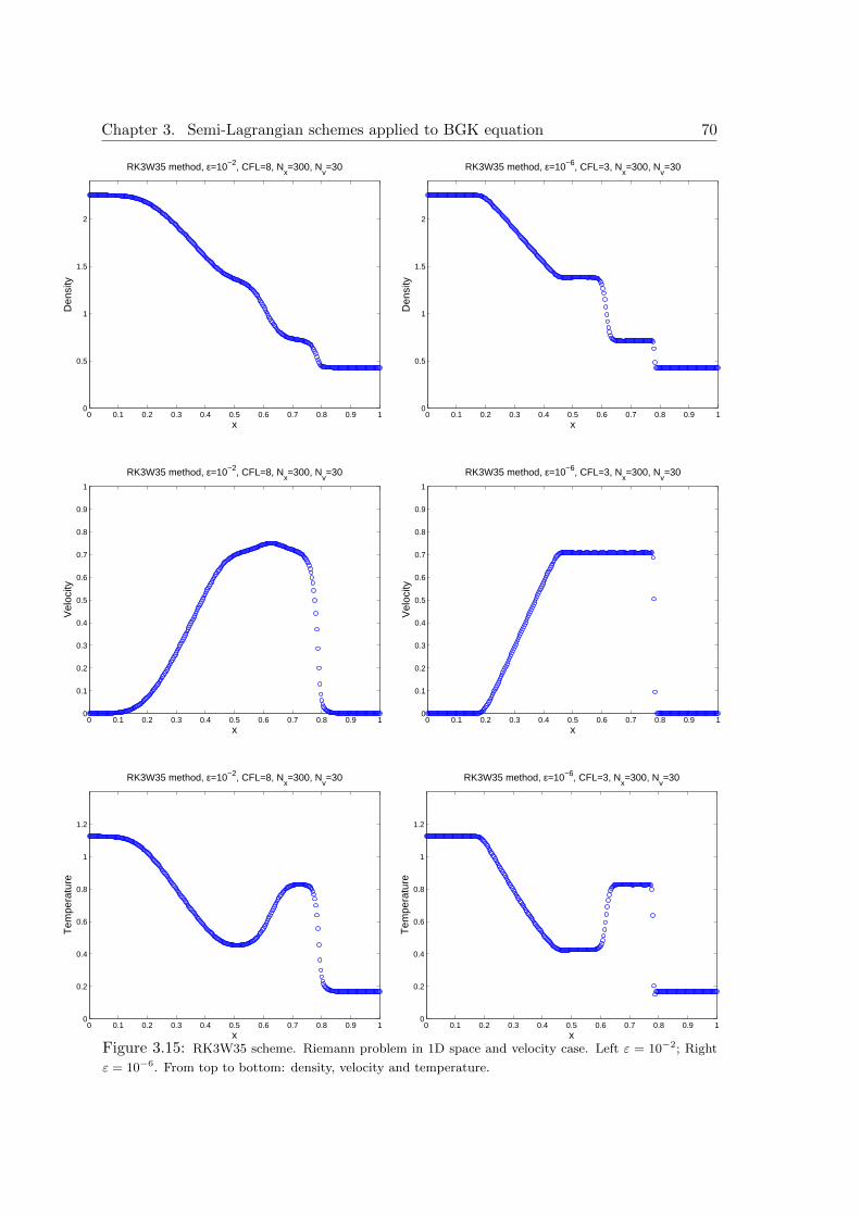
Chapter 3. Semi-Lagrangian schemes applied to BGK equation 70
0 0.1 0.2 0.3 0.4 0.5 0.6 0.7 0.8 0.9 10
0.5
1
1.5
2
RK3W35 method, ε=10−2, CFL=8, Nx=300, N
v=30
x
Den
sity
0 0.1 0.2 0.3 0.4 0.5 0.6 0.7 0.8 0.9 10
0.5
1
1.5
2
RK3W35 method, ε=10−6, CFL=3, Nx=300, N
v=30
x
Den
sity
0 0.1 0.2 0.3 0.4 0.5 0.6 0.7 0.8 0.9 10
0.1
0.2
0.3
0.4
0.5
0.6
0.7
0.8
0.9
1
RK3W35 method, ε=10−2, CFL=8, Nx=300, N
v=30
x
Vel
ocity
0 0.1 0.2 0.3 0.4 0.5 0.6 0.7 0.8 0.9 10
0.1
0.2
0.3
0.4
0.5
0.6
0.7
0.8
0.9
1
RK3W35 method, ε=10−6, CFL=3, Nx=300, N
v=30
x
Vel
ocity
0 0.1 0.2 0.3 0.4 0.5 0.6 0.7 0.8 0.9 10
0.2
0.4
0.6
0.8
1
1.2
RK3W35 method, ε=10−2, CFL=8, Nx=300, N
v=30
x
Tem
pera
ture
0 0.1 0.2 0.3 0.4 0.5 0.6 0.7 0.8 0.9 10
0.2
0.4
0.6
0.8
1
1.2
RK3W35 method, ε=10−6, CFL=3, Nx=300, N
v=30
x
Tem
pera
ture
Figure 3.15: RK3W35 scheme. Riemann problem in 1D space and velocity case. Left ε = 10−2; Right
ε = 10−6. From top to bottom: density, velocity and temperature.
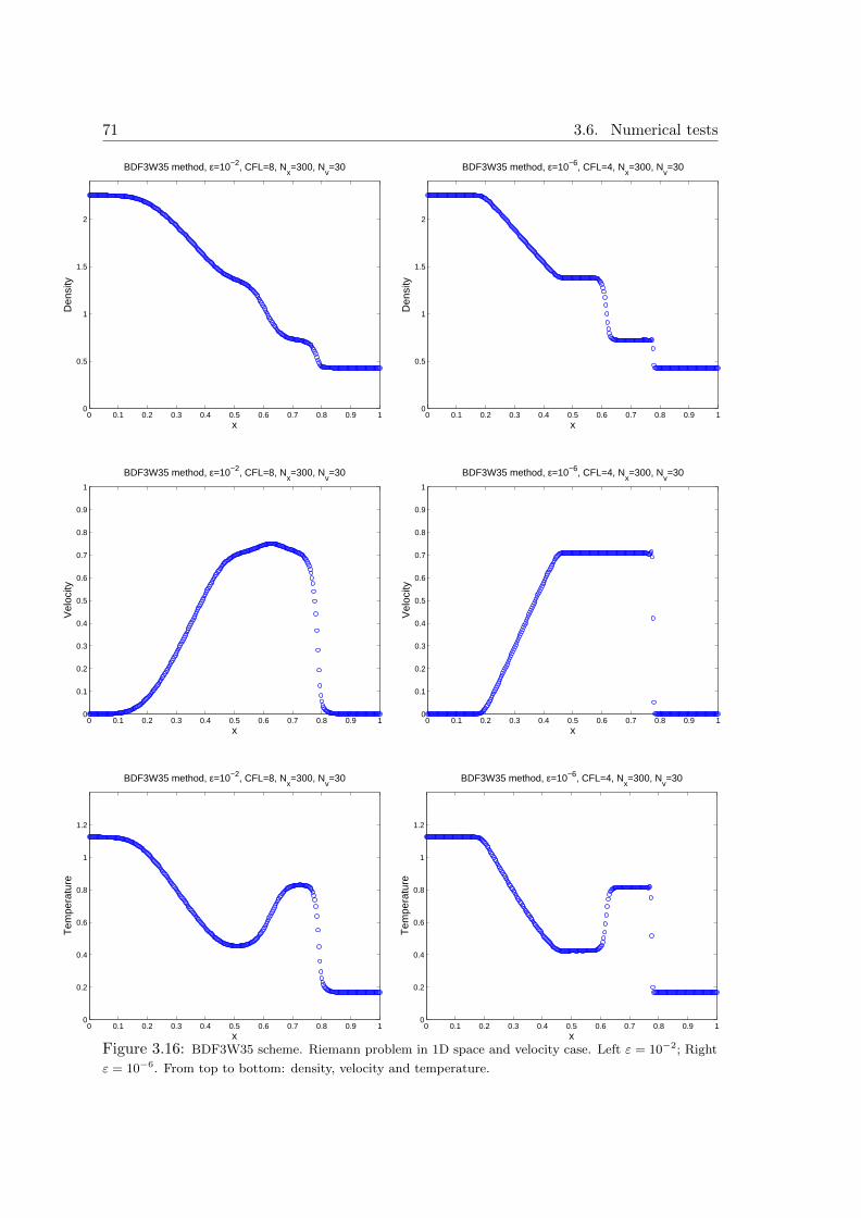
71 3.6. Numerical tests
0 0.1 0.2 0.3 0.4 0.5 0.6 0.7 0.8 0.9 10
0.5
1
1.5
2
BDF3W35 method, ε=10−2, CFL=8, Nx=300, N
v=30
x
Den
sity
0 0.1 0.2 0.3 0.4 0.5 0.6 0.7 0.8 0.9 10
0.5
1
1.5
2
BDF3W35 method, ε=10−6, CFL=4, Nx=300, N
v=30
x
Den
sity
0 0.1 0.2 0.3 0.4 0.5 0.6 0.7 0.8 0.9 10
0.1
0.2
0.3
0.4
0.5
0.6
0.7
0.8
0.9
1
BDF3W35 method, ε=10−2, CFL=8, Nx=300, N
v=30
x
Vel
ocity
0 0.1 0.2 0.3 0.4 0.5 0.6 0.7 0.8 0.9 10
0.1
0.2
0.3
0.4
0.5
0.6
0.7
0.8
0.9
1
BDF3W35 method, ε=10−6, CFL=4, Nx=300, N
v=30
x
Vel
ocity
0 0.1 0.2 0.3 0.4 0.5 0.6 0.7 0.8 0.9 10
0.2
0.4
0.6
0.8
1
1.2
BDF3W35 method, ε=10−2, CFL=8, Nx=300, N
v=30
x
Tem
pera
ture
0 0.1 0.2 0.3 0.4 0.5 0.6 0.7 0.8 0.9 10
0.2
0.4
0.6
0.8
1
1.2
BDF3W35 method, ε=10−6, CFL=4, Nx=300, N
v=30
x
Tem
pera
ture
Figure 3.16: BDF3W35 scheme. Riemann problem in 1D space and velocity case. Left ε = 10−2; Right
ε = 10−6. From top to bottom: density, velocity and temperature.
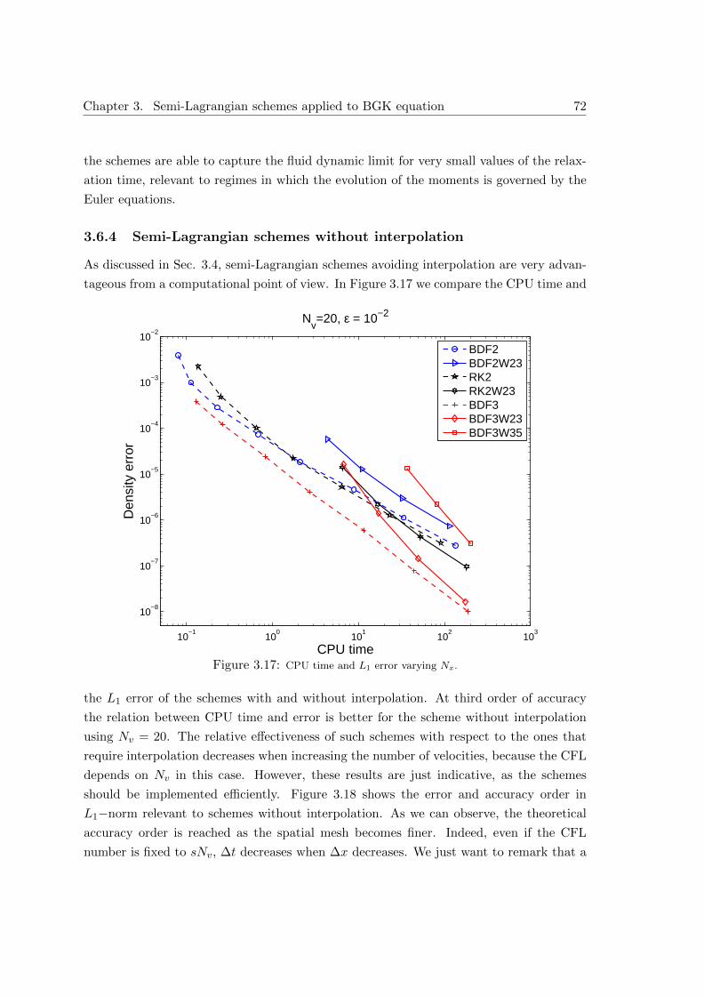
Chapter 3. Semi-Lagrangian schemes applied to BGK equation 72
the schemes are able to capture the fluid dynamic limit for very small values of the relax-
ation time, relevant to regimes in which the evolution of the moments is governed by the
Euler equations.
3.6.4 Semi-Lagrangian schemes without interpolation
As discussed in Sec. 3.4, semi-Lagrangian schemes avoiding interpolation are very advan-
tageous from a computational point of view. In Figure 3.17 we compare the CPU time and
10−1
100
101
102
103
10−8
10−7
10−6
10−5
10−4
10−3
10−2
Nv=20, ε = 10−2
CPU time
Den
sity
err
or
BDF2BDF2W23RK2RK2W23BDF3BDF3W23BDF3W35
Figure 3.17: CPU time and L1 error varying Nx.
the L1 error of the schemes with and without interpolation. At third order of accuracy
the relation between CPU time and error is better for the scheme without interpolation
using Nv = 20. The relative effectiveness of such schemes with respect to the ones that
require interpolation decreases when increasing the number of velocities, because the CFL
depends on Nv in this case. However, these results are just indicative, as the schemes
should be implemented efficiently. Figure 3.18 shows the error and accuracy order in
L1−norm relevant to schemes without interpolation. As we can observe, the theoretical
accuracy order is reached as the spatial mesh becomes finer. Indeed, even if the CFL
number is fixed to sNv, ∆t decreases when ∆x decreases. We just want to remark that a
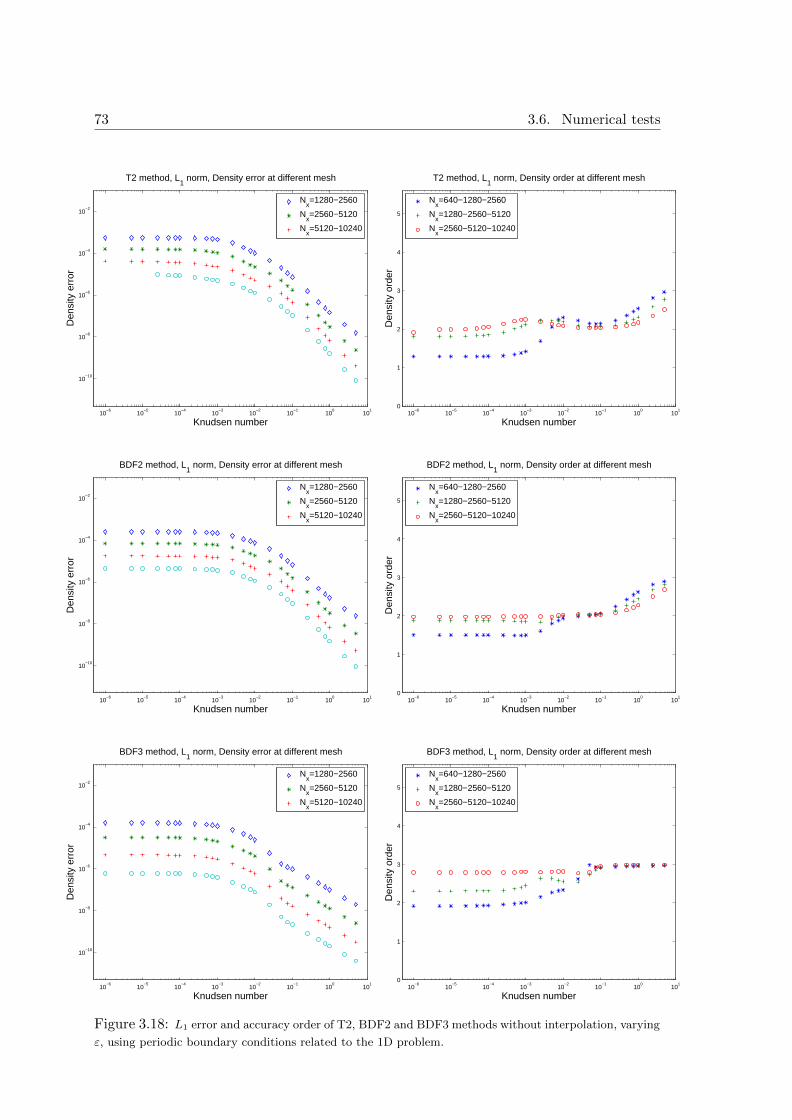
73 3.6. Numerical tests
10−6
10−5
10−4
10−3
10−2
10−1
100
101
10−10
10−8
10−6
10−4
10−2
T2 method, L1 norm, Density error at different mesh
Knudsen number
Den
sity
err
or
Nx=1280−2560
Nx=2560−5120
Nx=5120−10240
10−6
10−5
10−4
10−3
10−2
10−1
100
101
0
1
2
3
4
5
T2 method, L1 norm, Density order at different mesh
Knudsen number
Den
sity
ord
er
Nx=640−1280−2560
Nx=1280−2560−5120
Nx=2560−5120−10240
10−6
10−5
10−4
10−3
10−2
10−1
100
101
10−10
10−8
10−6
10−4
10−2
BDF2 method, L1 norm, Density error at different mesh
Knudsen number
Den
sity
err
or
Nx=1280−2560
Nx=2560−5120
Nx=5120−10240
10−6
10−5
10−4
10−3
10−2
10−1
100
101
0
1
2
3
4
5
BDF2 method, L1 norm, Density order at different mesh
Knudsen number
Den
sity
ord
er
Nx=640−1280−2560
Nx=1280−2560−5120
Nx=2560−5120−10240
10−6
10−5
10−4
10−3
10−2
10−1
100
101
10−10
10−8
10−6
10−4
10−2
BDF3 method, L1 norm, Density error at different mesh
Knudsen number
Den
sity
err
or
Nx=1280−2560
Nx=2560−5120
Nx=5120−10240
10−6
10−5
10−4
10−3
10−2
10−1
100
101
0
1
2
3
4
5
BDF3 method, L1 norm, Density order at different mesh
Knudsen number
Den
sity
ord
er
Nx=640−1280−2560
Nx=1280−2560−5120
Nx=2560−5120−10240
Figure 3.18: L1 error and accuracy order of T2, BDF2 and BDF3 methods without interpolation, varying
ε, using periodic boundary conditions related to the 1D problem.
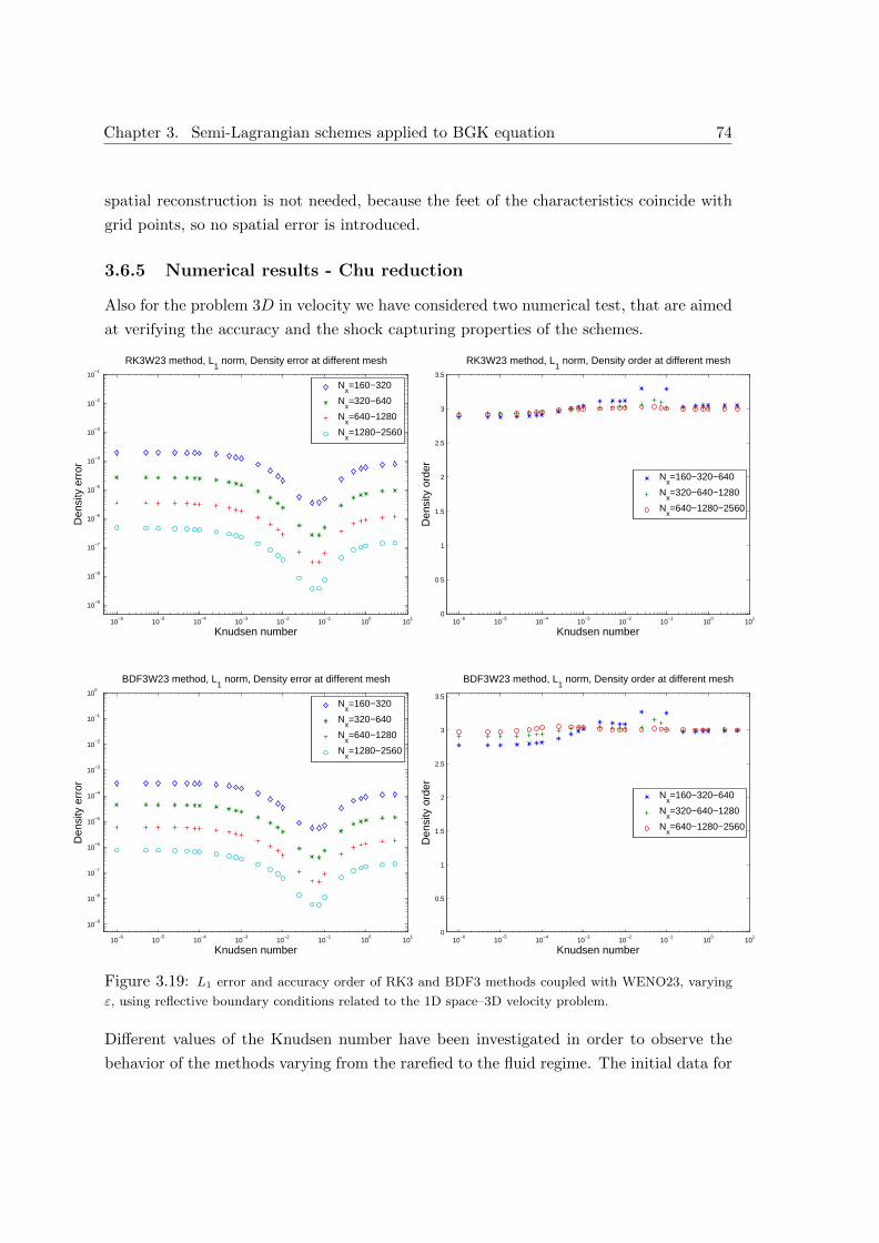
Chapter 3. Semi-Lagrangian schemes applied to BGK equation 74
spatial reconstruction is not needed, because the feet of the characteristics coincide with
grid points, so no spatial error is introduced.
3.6.5 Numerical results - Chu reduction
Also for the problem 3D in velocity we have considered two numerical test, that are aimed
at verifying the accuracy and the shock capturing properties of the schemes.
10−6
10−5
10−4
10−3
10−2
10−1
100
101
10−9
10−8
10−7
10−6
10−5
10−4
10−3
10−2
10−1
RK3W23 method, L1 norm, Density error at different mesh
Knudsen number
Den
sity
err
or
Nx=160−320
Nx=320−640
Nx=640−1280
Nx=1280−2560
10−6
10−5
10−4
10−3
10−2
10−1
100
101
0
0.5
1
1.5
2
2.5
3
3.5
RK3W23 method, L1 norm, Density order at different mesh
Knudsen number
Den
sity
ord
er
Nx=160−320−640
Nx=320−640−1280
Nx=640−1280−2560
10−6
10−5
10−4
10−3
10−2
10−1
100
101
10−9
10−8
10−7
10−6
10−5
10−4
10−3
10−2
10−1
100
BDF3W23 method, L1 norm, Density error at different mesh
Knudsen number
Den
sity
err
or
Nx=160−320
Nx=320−640
Nx=640−1280
Nx=1280−2560
10−6
10−5
10−4
10−3
10−2
10−1
100
101
0
0.5
1
1.5
2
2.5
3
3.5
BDF3W23 method, L1 norm, Density order at different mesh
Knudsen number
Den
sity
ord
er
Nx=160−320−640
Nx=320−640−1280
Nx=640−1280−2560
Figure 3.19: L1 error and accuracy order of RK3 and BDF3 methods coupled with WENO23, varying
ε, using reflective boundary conditions related to the 1D space–3D velocity problem.
Different values of the Knudsen number have been investigated in order to observe the
behavior of the methods varying from the rarefied to the fluid regime. The initial data for
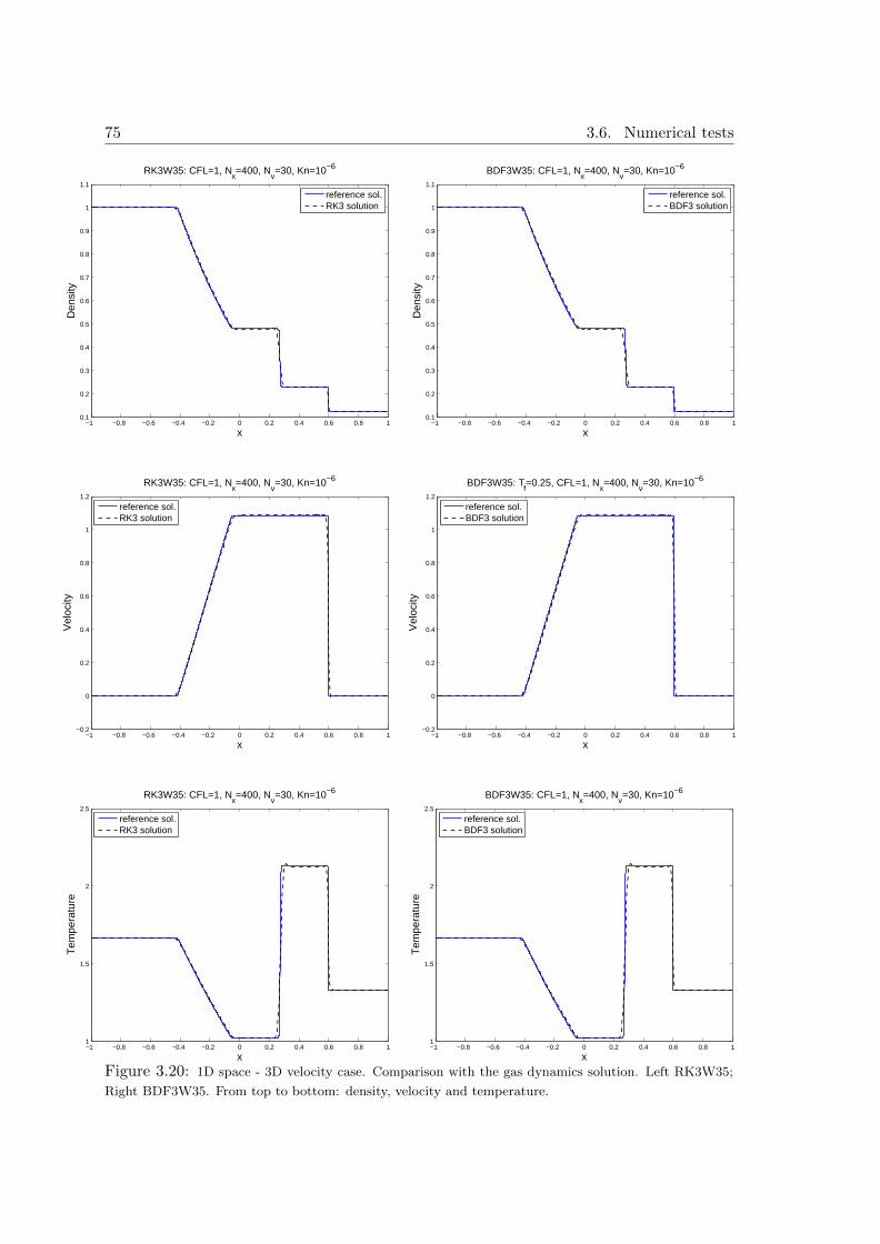
75 3.6. Numerical tests
−1 −0.8 −0.6 −0.4 −0.2 0 0.2 0.4 0.6 0.8 10.1
0.2
0.3
0.4
0.5
0.6
0.7
0.8
0.9
1
1.1
RK3W35: CFL=1, Nx=400, N
v=30, Kn=10−6
x
Den
sity
reference sol.RK3 solution
−1 −0.8 −0.6 −0.4 −0.2 0 0.2 0.4 0.6 0.8 10.1
0.2
0.3
0.4
0.5
0.6
0.7
0.8
0.9
1
1.1
BDF3W35: CFL=1, Nx=400, N
v=30, Kn=10−6
x
Den
sity
reference sol.BDF3 solution
−1 −0.8 −0.6 −0.4 −0.2 0 0.2 0.4 0.6 0.8 1−0.2
0
0.2
0.4
0.6
0.8
1
1.2
RK3W35: CFL=1, Nx=400, N
v=30, Kn=10−6
x
Vel
ocity
reference sol.RK3 solution
−1 −0.8 −0.6 −0.4 −0.2 0 0.2 0.4 0.6 0.8 1−0.2
0
0.2
0.4
0.6
0.8
1
1.2
BDF3W35: Tf=0.25, CFL=1, N
x=400, N
v=30, Kn=10−6
x
Vel
ocity
reference sol.BDF3 solution
−1 −0.8 −0.6 −0.4 −0.2 0 0.2 0.4 0.6 0.8 11
1.5
2
2.5
RK3W35: CFL=1, Nx=400, N
v=30, Kn=10−6
x
Tem
pera
ture
reference sol.RK3 solution
−1 −0.8 −0.6 −0.4 −0.2 0 0.2 0.4 0.6 0.8 11
1.5
2
2.5
BDF3W35: CFL=1, Nx=400, N
v=30, Kn=10−6
x
Tem
pera
ture
reference sol.BDF3 solution
Figure 3.20: 1D space - 3D velocity case. Comparison with the gas dynamics solution. Left RK3W35;
Right BDF3W35. From top to bottom: density, velocity and temperature.
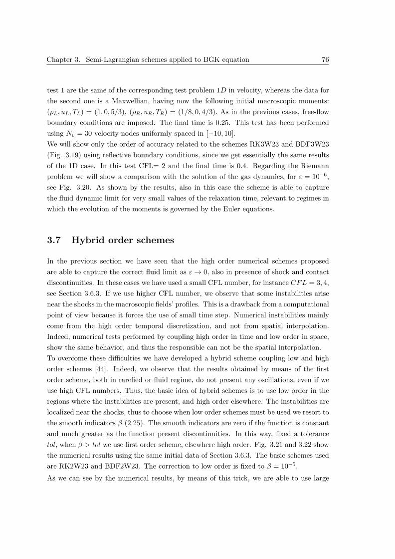
Chapter 3. Semi-Lagrangian schemes applied to BGK equation 76
test 1 are the same of the corresponding test problem 1D in velocity, whereas the data for
the second one is a Maxwellian, having now the following initial macroscopic moments:
(ρL, uL, TL) = (1, 0, 5/3), (ρR, uR, TR) = (1/8, 0, 4/3). As in the previous cases, free-flow
boundary conditions are imposed. The final time is 0.25. This test has been performed
using Nv = 30 velocity nodes uniformly spaced in [−10, 10].
We will show only the order of accuracy related to the schemes RK3W23 and BDF3W23
(Fig. 3.19) using reflective boundary conditions, since we get essentially the same results
of the 1D case. In this test CFL= 2 and the final time is 0.4. Regarding the Riemann
problem we will show a comparison with the solution of the gas dynamics, for ε = 10−6,
see Fig. 3.20. As shown by the results, also in this case the scheme is able to capture
the fluid dynamic limit for very small values of the relaxation time, relevant to regimes in
which the evolution of the moments is governed by the Euler equations.
3.7 Hybrid order schemes
In the previous section we have seen that the high order numerical schemes proposed
are able to capture the correct fluid limit as ε→ 0, also in presence of shock and contact
discontinuities. In these cases we have used a small CFL number, for instance CFL = 3, 4,
see Section 3.6.3. If we use higher CFL number, we observe that some instabilities arise
near the shocks in the macroscopic fields’ profiles. This is a drawback from a computational
point of view because it forces the use of small time step. Numerical instabilities mainly
come from the high order temporal discretization, and not from spatial interpolation.
Indeed, numerical tests performed by coupling high order in time and low order in space,
show the same behavior, and thus the responsible can not be the spatial interpolation.
To overcome these difficulties we have developed a hybrid scheme coupling low and high
order schemes [44]. Indeed, we observe that the results obtained by means of the first
order scheme, both in rarefied or fluid regime, do not present any oscillations, even if we
use high CFL numbers. Thus, the basic idea of hybrid schemes is to use low order in the
regions where the instabilities are present, and high order elsewhere. The instabilities are
localized near the shocks, thus to choose when low order schemes must be used we resort to
the smooth indicators β (2.25). The smooth indicators are zero if the function is constant
and much greater as the function present discontinuities. In this way, fixed a tolerance
tol, when β > tol we use first order scheme, elsewhere high order. Fig. 3.21 and 3.22 show
the numerical results using the same initial data of Section 3.6.3. The basic schemes used
are RK2W23 and BDF2W23. The correction to low order is fixed to β = 10−5.
As we can see by the numerical results, by means of this trick, we are able to use large
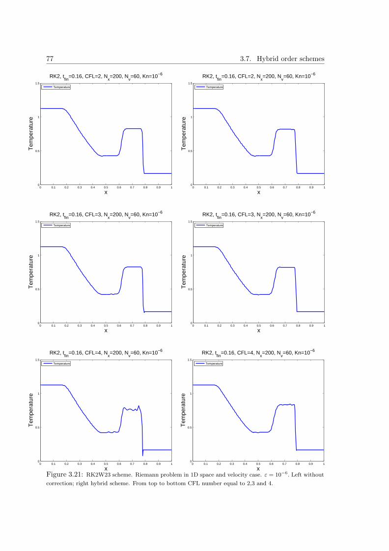
77 3.7. Hybrid order schemes
0 0.1 0.2 0.3 0.4 0.5 0.6 0.7 0.8 0.9 10
0.5
1
1.5
RK2, tfin
=0.16, CFL=2, Nx=200, N
v=60, Kn=10−6
x
Tem
pera
ture
Temperature
0 0.1 0.2 0.3 0.4 0.5 0.6 0.7 0.8 0.9 10
0.5
1
1.5
RK2, tfin
=0.16, CFL=2, Nx=200, N
v=60, Kn=10−6
x
Tem
pera
ture
Temperature
0 0.1 0.2 0.3 0.4 0.5 0.6 0.7 0.8 0.9 10
0.5
1
1.5
RK2, tfin
=0.16, CFL=3, Nx=200, N
v=60, Kn=10−6
x
Tem
pera
ture
Temperature
0 0.1 0.2 0.3 0.4 0.5 0.6 0.7 0.8 0.9 10
0.5
1
1.5
RK2, tfin
=0.16, CFL=3, Nx=200, N
v=60, Kn=10−6
x
Tem
pera
ture
Temperature
0 0.1 0.2 0.3 0.4 0.5 0.6 0.7 0.8 0.9 10
0.5
1
1.5
RK2, tfin
=0.16, CFL=4, Nx=200, N
v=60, Kn=10−6
x
Tem
pera
ture
Temperature
0 0.1 0.2 0.3 0.4 0.5 0.6 0.7 0.8 0.9 10
0.5
1
1.5
RK2, tfin
=0.16, CFL=4, Nx=200, N
v=60, Kn=10−6
x
Tem
pera
ture
Temperature
Figure 3.21: RK2W23 scheme. Riemann problem in 1D space and velocity case. ε = 10−6. Left without
correction; right hybrid scheme. From top to bottom CFL number equal to 2,3 and 4.
Chapter 3. Semi-Lagrangian schemes applied to BGK equation 78
0 0.1 0.2 0.3 0.4 0.5 0.6 0.7 0.8 0.9 10
0.5
1
1.5
BDF2, tfin
=0.16, CFL=2, Nx=200, N
v=60, Kn=10−6
x
Tem
pera
ture
Temperature
0 0.1 0.2 0.3 0.4 0.5 0.6 0.7 0.8 0.9 10
0.5
1
1.5
BDF2, tfin
=0.16, CFL=2, Nx=200, N
v=60, Kn=10−6
x
Tem
pera
ture
Temperature
0 0.1 0.2 0.3 0.4 0.5 0.6 0.7 0.8 0.9 10
0.5
1
1.5
BDF2, tfin
=0.16, CFL=4, Nx=200, N
v=60, Kn=10−6
x
Tem
pera
ture
Temperature
0 0.1 0.2 0.3 0.4 0.5 0.6 0.7 0.8 0.9 10
0.5
1
1.5
BDF2, tfin
=0.16, CFL=4, Nx=200, N
v=60, Kn=10−6
x
Tem
pera
ture
Temperature
0 0.1 0.2 0.3 0.4 0.5 0.6 0.7 0.8 0.9 10
0.5
1
1.5
BDF2, tfin
=0.16, CFL=8, Nx=200, N
v=60, Kn=10−6
x
Tem
pera
ture
Temperature
0 0.1 0.2 0.3 0.4 0.5 0.6 0.7 0.8 0.9 10
0.5
1
1.5
BDF2, tfin
=0.16, CFL=8, Nx=200, N
v=60, Kn=10−6
x
Tem
pera
ture
Temperature
Figure 3.22: BDF2W23 scheme. Riemann problem in 1D space and velocity case. ε = 10−6. Left
without correction; right hybrid scheme. From top to bottom CFL number equal to 2,4 and 8.
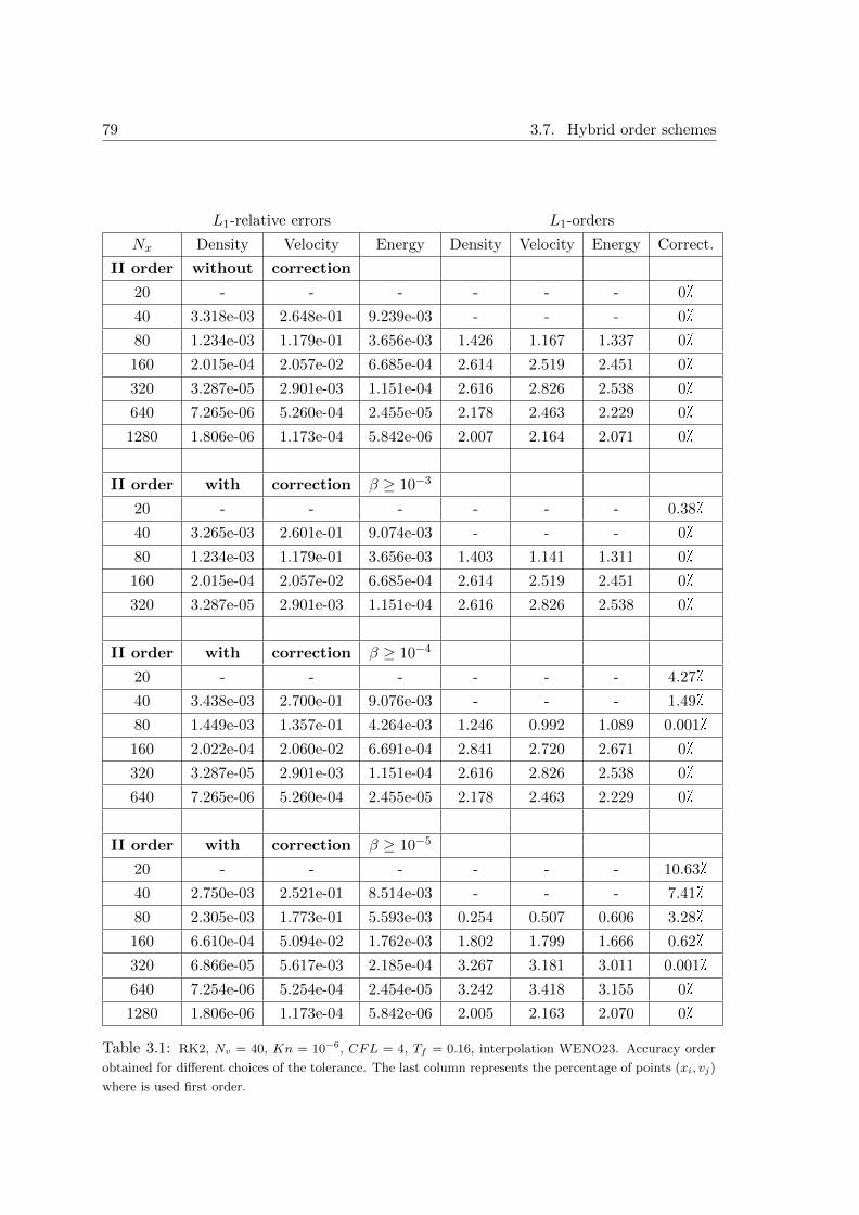
79 3.7. Hybrid order schemes
L1-relative errors L1-orders
Nx Density Velocity Energy Density Velocity Energy Correct.
II order without correction
20 - - - - - - 0
40 3.318e-03 2.648e-01 9.239e-03 - - - 0
80 1.234e-03 1.179e-01 3.656e-03 1.426 1.167 1.337 0
160 2.015e-04 2.057e-02 6.685e-04 2.614 2.519 2.451 0
320 3.287e-05 2.901e-03 1.151e-04 2.616 2.826 2.538 0
640 7.265e-06 5.260e-04 2.455e-05 2.178 2.463 2.229 0
1280 1.806e-06 1.173e-04 5.842e-06 2.007 2.164 2.071 0
II order with correction β ≥ 10−3
20 - - - - - - 0.38
40 3.265e-03 2.601e-01 9.074e-03 - - - 0
80 1.234e-03 1.179e-01 3.656e-03 1.403 1.141 1.311 0
160 2.015e-04 2.057e-02 6.685e-04 2.614 2.519 2.451 0
320 3.287e-05 2.901e-03 1.151e-04 2.616 2.826 2.538 0
II order with correction β ≥ 10−4
20 - - - - - - 4.27
40 3.438e-03 2.700e-01 9.076e-03 - - - 1.49
80 1.449e-03 1.357e-01 4.264e-03 1.246 0.992 1.089 0.001
160 2.022e-04 2.060e-02 6.691e-04 2.841 2.720 2.671 0
320 3.287e-05 2.901e-03 1.151e-04 2.616 2.826 2.538 0
640 7.265e-06 5.260e-04 2.455e-05 2.178 2.463 2.229 0
II order with correction β ≥ 10−5
20 - - - - - - 10.63
40 2.750e-03 2.521e-01 8.514e-03 - - - 7.41
80 2.305e-03 1.773e-01 5.593e-03 0.254 0.507 0.606 3.28
160 6.610e-04 5.094e-02 1.762e-03 1.802 1.799 1.666 0.62
320 6.866e-05 5.617e-03 2.185e-04 3.267 3.181 3.011 0.001
640 7.254e-06 5.254e-04 2.454e-05 3.242 3.418 3.155 0
1280 1.806e-06 1.173e-04 5.842e-06 2.005 2.163 2.070 0
Table 3.1: RK2, Nv = 40, Kn = 10−6, CFL = 4, Tf = 0.16, interpolation WENO23. Accuracy order
obtained for different choices of the tolerance. The last column represents the percentage of points (xi, vj)
where is used first order.
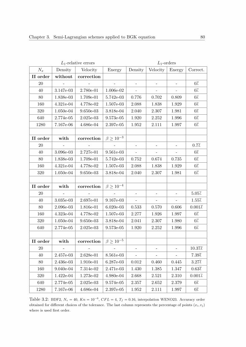
Chapter 3. Semi-Lagrangian schemes applied to BGK equation 80
L1-relative errors L1-orders
Nx Density Velocity Energy Density Velocity Energy Correct.
II order without correction
20 - - - - - - 0
40 3.147e-03 2.780e-01 1.006e-02 - - - 0
80 1.838e-03 1.709e-01 5.742e-03 0.776 0.702 0.809 0
160 4.321e-04 4.778e-02 1.507e-03 2.088 1.838 1.929 0
320 1.050e-04 9.650e-03 3.818e-04 2.040 2.307 1.981 0
640 2.774e-05 2.025e-03 9.573e-05 1.920 2.252 1.996 0
1280 7.167e-06 4.686e-04 2.397e-05 1.952 2.111 1.997 0
II order with correction β ≥ 10−3
20 - - - - - - 0.7
40 3.096e-03 2.727e-01 9.561e-03 - - - 0
80 1.838e-03 1.709e-01 5.742e-03 0.752 0.674 0.735 0
160 4.321e-04 4.778e-02 1.507e-03 2.088 1.838 1.929 0
320 1.050e-04 9.650e-03 3.818e-04 2.040 2.307 1.981 0
II order with correction β ≥ 10−4
20 - - - - - - 5.05
40 3.035e-03 2.697e-01 9.167e-03 - - - 1.55
80 2.096e-03 1.816e-01 6.020e-03 0.533 0.570 0.606 0.001
160 4.323e-04 4.778e-02 1.507e-03 2.277 1.926 1.997 0
320 1.050e-04 9.650e-03 3.818e-04 2.041 2.307 1.980 0
640 2.774e-05 2.025e-03 9.573e-05 1.920 2.252 1.996 0
II order with correction β ≥ 10−5
20 - - - - - - 10.37
40 2.457e-03 2.628e-01 8.561e-03 - - - 7.39
80 2.436e-03 1.910e-01 6.287e-03 0.012 0.460 0.445 3.27
160 9.040e-04 7.314e-02 2.471e-03 1.430 1.385 1.347 0.63
320 1.422e-04 1.273e-02 4.980e-04 2.668 2.521 2.310 0.001
640 2.774e-05 2.025e-03 9.574e-05 2.357 2.652 2.379 0
1280 7.167e-06 4.686e-04 2.397e-05 1.952 2.111 1.997 0
Table 3.2: BDF2, Nv = 40, Kn = 10−6, CFL = 4, Tf = 0.16, interpolation WENO23. Accuracy order
obtained for different choices of the tolerance. The last column represents the percentage of points (xi, vj)
where is used first order.
81 3.7. Hybrid order schemes
time step also in fluid regimes. Of course, one may ask: how much does accuracy order
decrease? Tables 3.1 and 3.2 show the accuracy orders of the same hybrid schemes applied
to a smooth initial data using different tolerance. We can observe a small degradation of
the accuracy order. However, increasing the number of grid points, the schemes tend to
avoid corrections to first order and high order is recovered. Therefore, we can conclude
that, using large time step together order reduction, we lose a bit of accuracy, but we
obtain a numerical scheme that does not present oscillation.

Chapter 3. Semi-Lagrangian schemes applied to BGK equation 82
Chapter 4
Gas-surface interaction and
boundary conditions
In many applications the gas moves in a region bounded by one or several solid bodies,
and in these cases boundary conditions have to be prescribed to characterize the behavior
of the gas near the wall. In the following sections we shall investigate the conditions which
must be satisfied by the distribution function f at the boundary ∂D of the region D where
the motion of the particles takes place. The theoretical investigations of the gas-wall in-
teraction are exceedingly difficult because of the complexity of phenomena taking place at
the wall.
In this thesis we refer to the boundary conditions proposed by Maxwell. In a appendix to a
paper published in 1879 [13, 35] he discussed the problem of finding a boundary condition
for the distribution function. As a first hypothesis he supposed the surface of a physical
wall to be a perfectly elastic smooth fixed surface, having the apparent shape of the solid
without any minute deviations. In this case the gas molecules are reflected in a specular
way; therefore the gas cannot exert any stress on the surface, except in the direction of
the normal. The condition read as:
fs = f(t, x, v) = f(t, x, v − 2n(n · (v − vb))), x ∈ ∂D, (v − vb) · n > 0, (4.1)
where n is the unit vector normal to the surface at x and vb is the velocity of the wall,
which is non zero if we are dealing with a moving boundary.
Maxwell noticed that assumption (4.1), known as specular reflection boundary condition,
means that the gas can exert any stress on the surface only in the direction of the normal.
This assumption is extremely unrealistic and can only be used in particular cases, since
in many situations the gas can exert stresses also in oblique directions to the surface, that
83
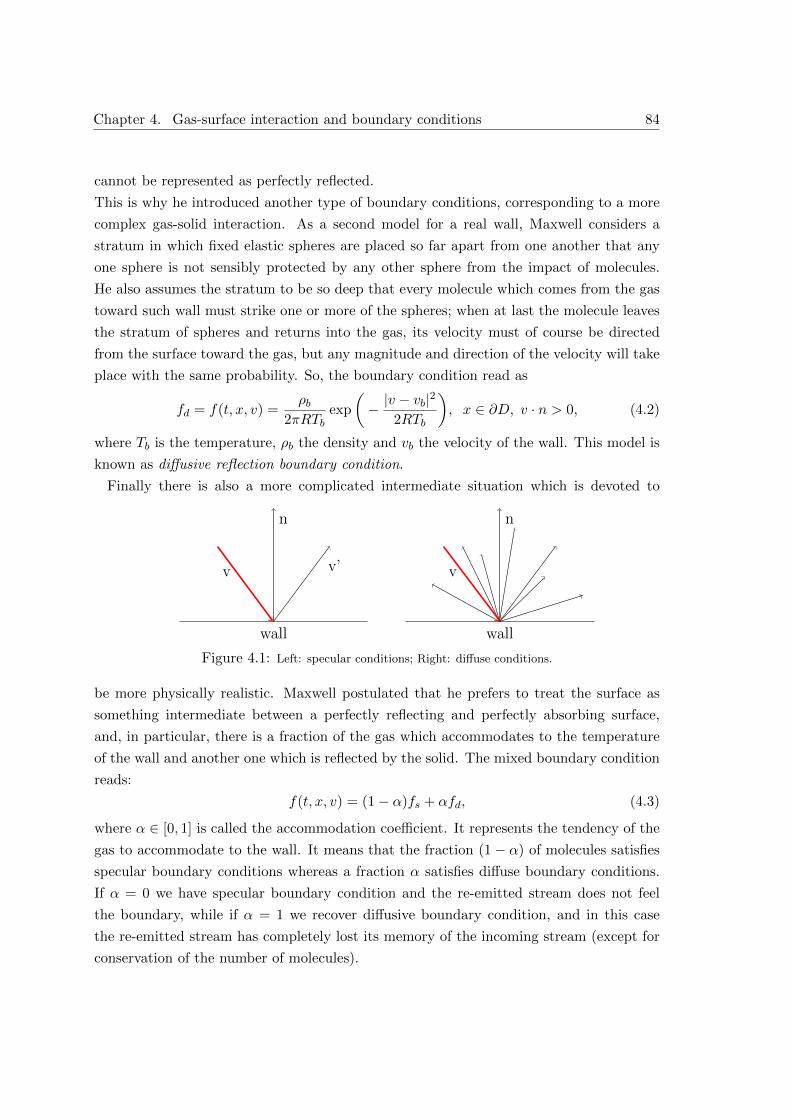
Chapter 4. Gas-surface interaction and boundary conditions 84
cannot be represented as perfectly reflected.
This is why he introduced another type of boundary conditions, corresponding to a more
complex gas-solid interaction. As a second model for a real wall, Maxwell considers a
stratum in which fixed elastic spheres are placed so far apart from one another that any
one sphere is not sensibly protected by any other sphere from the impact of molecules.
He also assumes the stratum to be so deep that every molecule which comes from the gas
toward such wall must strike one or more of the spheres; when at last the molecule leaves
the stratum of spheres and returns into the gas, its velocity must of course be directed
from the surface toward the gas, but any magnitude and direction of the velocity will take
place with the same probability. So, the boundary condition read as
fd = f(t, x, v) =ρb
2πRTbexp
(− |v − vb|
2
2RTb
), x ∈ ∂D, v · n > 0, (4.2)
where Tb is the temperature, ρb the density and vb the velocity of the wall. This model is
known as diffusive reflection boundary condition.
Finally there is also a more complicated intermediate situation which is devoted to
wall
n
v v’
wall
n
v
Figure 4.1: Left: specular conditions; Right: diffuse conditions.
be more physically realistic. Maxwell postulated that he prefers to treat the surface as
something intermediate between a perfectly reflecting and perfectly absorbing surface,
and, in particular, there is a fraction of the gas which accommodates to the temperature
of the wall and another one which is reflected by the solid. The mixed boundary condition
reads:
f(t, x, v) = (1− α)fs + αfd, (4.3)
where α ∈ [0, 1] is called the accommodation coefficient. It represents the tendency of the
gas to accommodate to the wall. It means that the fraction (1− α) of molecules satisfies
specular boundary conditions whereas a fraction α satisfies diffuse boundary conditions.
If α = 0 we have specular boundary condition and the re-emitted stream does not feel
the boundary, while if α = 1 we recover diffusive boundary condition, and in this case
the re-emitted stream has completely lost its memory of the incoming stream (except for
conservation of the number of molecules).
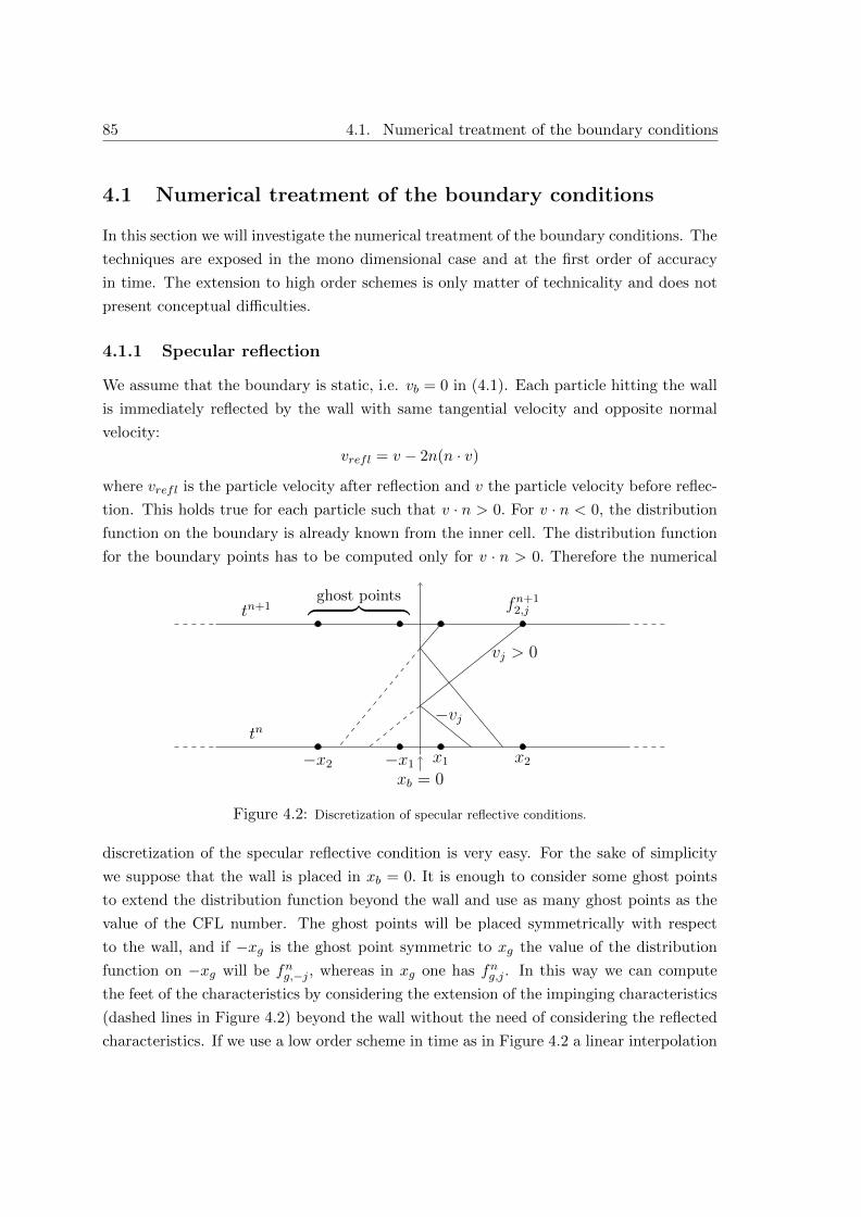
85 4.1. Numerical treatment of the boundary conditions
4.1 Numerical treatment of the boundary conditions
In this section we will investigate the numerical treatment of the boundary conditions. The
techniques are exposed in the mono dimensional case and at the first order of accuracy
in time. The extension to high order schemes is only matter of technicality and does not
present conceptual difficulties.
4.1.1 Specular reflection
We assume that the boundary is static, i.e. vb = 0 in (4.1). Each particle hitting the wall
is immediately reflected by the wall with same tangential velocity and opposite normal
velocity:
vrefl = v − 2n(n · v)
where vrefl is the particle velocity after reflection and v the particle velocity before reflec-
tion. This holds true for each particle such that v · n > 0. For v · n < 0, the distribution
function on the boundary is already known from the inner cell. The distribution function
for the boundary points has to be computed only for v · n > 0. Therefore the numerical
vj > 0
−vj
xb = 0
x1 x2−x1−x2
tn
tn+1 fn+12,j
ghost points︷ ︸︸ ︷
Figure 4.2: Discretization of specular reflective conditions.
discretization of the specular reflective condition is very easy. For the sake of simplicity
we suppose that the wall is placed in xb = 0. It is enough to consider some ghost points
to extend the distribution function beyond the wall and use as many ghost points as the
value of the CFL number. The ghost points will be placed symmetrically with respect
to the wall, and if −xg is the ghost point symmetric to xg the value of the distribution
function on −xg will be fng,−j , whereas in xg one has fng,j . In this way we can compute
the feet of the characteristics by considering the extension of the impinging characteristics
(dashed lines in Figure 4.2) beyond the wall without the need of considering the reflected
characteristics. If we use a low order scheme in time as in Figure 4.2 a linear interpolation
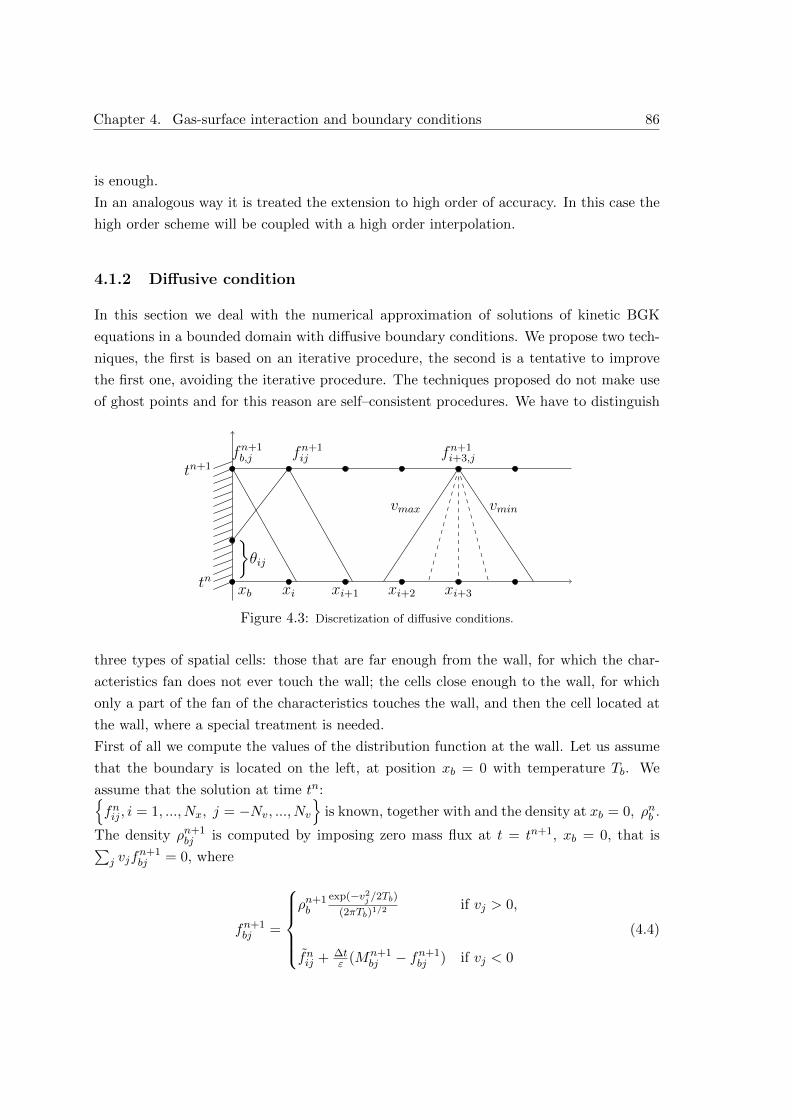
Chapter 4. Gas-surface interaction and boundary conditions 86
is enough.
In an analogous way it is treated the extension to high order of accuracy. In this case the
high order scheme will be coupled with a high order interpolation.
4.1.2 Diffusive condition
In this section we deal with the numerical approximation of solutions of kinetic BGK
equations in a bounded domain with diffusive boundary conditions. We propose two tech-
niques, the first is based on an iterative procedure, the second is a tentative to improve
the first one, avoiding the iterative procedure. The techniques proposed do not make use
of ghost points and for this reason are self–consistent procedures. We have to distinguish
xi xi+1 xi+2 xi+3xbtn
tn+1fn+1ij fn+1
i+3,jfn+1b,j
θij
vmax vmin
Figure 4.3: Discretization of diffusive conditions.
three types of spatial cells: those that are far enough from the wall, for which the char-
acteristics fan does not ever touch the wall; the cells close enough to the wall, for which
only a part of the fan of the characteristics touches the wall, and then the cell located at
the wall, where a special treatment is needed.
First of all we compute the values of the distribution function at the wall. Let us assume
that the boundary is located on the left, at position xb = 0 with temperature Tb. We
assume that the solution at time tn:fnij , i = 1, ..., Nx, j = −Nv, ..., Nv
is known, together with and the density at xb = 0, ρnb .
The density ρn+1bj is computed by imposing zero mass flux at t = tn+1, xb = 0, that is∑
j vjfn+1bj = 0, where
fn+1bj =
ρn+1b
exp(−v2j /2Tb)(2πTb)1/2
if vj > 0,
fnij + ∆tε (Mn+1
bj − fn+1bj ) if vj < 0
(4.4)
87 4.1. Numerical treatment of the boundary conditions
The Maxwellian Mn+1bj cannot be computed in the usual way. We shall therefore use an
iterative procedure. Let
f(0)bj =
ρ(0)b Ebj for vj > 0,
fnij = f(tn, xi − vj∆t, vj) for vj < 0
with Ebj = exp(−v2j /2Tb)/(2πTb)
1/2. Imposing∑
j vjf(0)bj = 0 one determines ρ(0). Once
ρ(0) is known, one computes the moments m(0)β =
∑j v
βj f
(0)bj , β = 0, 1, 2. From the
moments one computes the Maxwellian M(0)bj . Then one can iterate untill convergence:
f(k)bj =
ρ(k)b Ebj if vj > 0,
fnij + ∆tε (M
(k−1)bj − f (k−1)
bj ) if vj < 0
Finally we set fn+1bj = limk→∞ f
(k)bj and ρn+1
b = limk→∞ ρ(k)b . Once the density at the new
time tn+1 has been found, one can then compute the function at other grid points, as
follows. Let us consider, for example, point xi in the previous figure. Then one has:
fn+1ij =
fnij + ∆tε (Mn+1
ij − fn+1ij ) if xij = xi − vj∆t > 0,
fθij =(θijρ
n+1b + (1− θij)ρnb
)Ebj if xij < 0.
(4.5)
The geometrical factor θij = 1− xi/(vj∆t) can be computed for each velocity.
The Maxwellian Mn+1ij may be computed by using an iterative procedure similar to the
one used for the computation of ρn+1b . Starting from
f(0)ij =
fnij if xij > 0,
fθij if xij < 0,
one computes the moments m(0)β =
∑j v
βj f
(0)ij and then M
(0)ij . Given f
(k−1)ij , compute
f(k)ij =
fnij + ∆tε (M
(k−1)ij − f (k−1)
ij ) if xij > 0,
fθij +(1−θij)∆t
ε (M(k−1)ij − f (k−1)
ij ) if xij < 0.
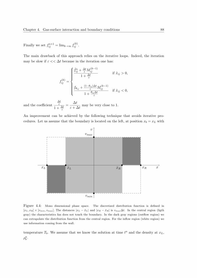
Chapter 4. Gas-surface interaction and boundary conditions 88
Finally we set fn+1ij = limk→∞ f
(k)ij .
The main drawback of this approach relies on the iterative loops. Indeed, the iteration
may be slow if ε << ∆t because in the iteration one has:
f(k)ij =
fnij + ∆tε M
(k−1)ij
1 + ∆tε
if xij > 0,
fθij +(1−θij)∆t
ε M(k−1)ij
1 +θij∆tε
if xij < 0,
and the coefficient∆tε
1 + ∆tε
=∆t
ε+ ∆tmay be very close to 1.
An improvement can be achieved by the following technique that avoids iterative pro-
cedures. Let us assume that the boundary is located on the left, at position xb = xL with
xL xR x
v
vmin
vmax
xL xR
Figure 4.4: Mono dimensional phase space. The discretized distribution function is defined in
[xL, xR] × [vmin, vmax]. The distances |xL − xL| and |xR − xR| is vmax∆t. In the central region (ligth
gray) the characteristics fan does not touch the boundary. In the dark gray regions (outflow region) we
can extrapolate the distribution function from the central region. For the inflow region (white region) we
use information coming from the wall.
temperature Tb. We assume that we know the solution at time tn and the density at xL,
ρnb .
89 4.1. Numerical treatment of the boundary conditions
First of all we can compute the distribution function at time tn+1 where the characteris-
tics fan does not touch the wall (light gray region, Fig. 4.4) using the technique described
in the previous chapter. Then one can compute the distribution function at the outflow
region (dark gray region, Fig. 4.4), where v · n < 0, for the spatial grid nodes whose
characteristics fan touches the wall, by extrapolation. A natural way to extrapolate the
distribution function is by means of Lagrange polynomials. However, when a shock goes
out of the boundary, the high order extrapolation may lead to severe oscillations near the
shock. To prevent this, we would like to have a lower order accurate but more robust ex-
trapolation. Therefore, a WENO type extrapolation [19, 54] will be applied and described
in the next section.
Now, we can compute the distribution function at the inflow boundary in a very sim-
ple way making a little modification to the expression (4.4). We define the distribution
function at the boundary in this way:
fn+1bj =
fn+1bj (obtained by extrap.) if vj · n < 0
ρn+1b Ebj if vj · n > 0.
(4.6)
The main difference between expressions (4.4) and (4.6) is that in expression (4.6) the
Maxwellian at time tn+1 does not appear, therefore there is no need for iterative loops.
The unknown is only ρn+1b , that can be easily computed imposing zero mass flux at the
boundary:
ρn+1b =
∑vj ·n<0 vjf
n+1bj∑
vj ·n>0 vjEbj. (4.7)
As last, we have to update the distribution function at time tn+1 in the spatial grid nodes
whose characteristics fan touches the wall at the inflow (white region, Fig. 4.4). In this
case we define the distribution function in the following way:
fn+1ij =
fn+1ij (obtained by extrap.) if vj · n < 0
fθij if vj · n > 0 and xij < 0.
interpolation betweenfθijand
fnij in the inner cells (light gray region) if vj · n > 0 and xij > 0.
(4.8)
Also in this case the main difference between expressions (4.5) and (4.8) is that in expres-
sion (4.6) the Maxwellian at time tn+1 does not appear, therefore there is again no need
Chapter 4. Gas-surface interaction and boundary conditions 90
for iterative loops to compute the macroscopic moments of the Maxwellian.
The main advantage of the second technique is that the computational time does not in-
crease as the relaxation parameter approaches to zero, but remains constant. Moreover,
the formulation is self consistent (mass conservation is maintained), and the numerical
technique explained in Fig. 4.4 has to be used only for few grid points near the boundary.
4.2 Inverse Lax-Wendroff technique
A good technique available in literature to treat diffusive boundary conditions due to Filbet
and Yang [19], is the Inverse Lax-Wendroff method. This technique is useful when the
numerical scheme foresees the employment of ghost points. In particular, it is applied to
compute the values of f at the ghost points for the inflow boundary. In this case we cannot
approximate f by an extrapolation, since the distribution function at the interior points
cannot predict the inflow. Filbet and Yang in [19] extended the inverse Lax-Wendroff type
procedure proposed in [55, 30, 59] for solving kinetic equations. At the left boundary xL,
a first order Taylor expansion gives
fj(x) = fxL,j + (x− xL)∂f
∂x
∣∣∣∣x=xL
+O(∆x2).
Hence a first order approximation of f at ghost points g is
fg,j = fxL,j + (xg − xL)∂f
∂x
∣∣∣∣x=xL
.
To obtain the values on the ghost points it is necessary to approximate the first spatial
derivative. By reformulating the Boltzmann equation we have
∂f
∂x
∣∣∣∣x=xL
=1
vx
(− ∂f
∂t+
1
εQ(f, f)
)∣∣∣∣x=xL
.
Now, instead of approximating the first spatial derivative, one has to compute the time
derivative and the collision operator in x = xL. An approximation of the time derivative
and of the collision term can be computed explicitly using the values of f at previous
time instants at the boundary. In the numerical test section a comparison between the
technique proposed in this thesis and the inverse Lax-Wendroff method is investigated.
4.3 Numerical test
In this section, we present a variety of test cases in 1D showing the effectiveness of our
method to get an accurate solution of the BGK equation set in a bounded domain with
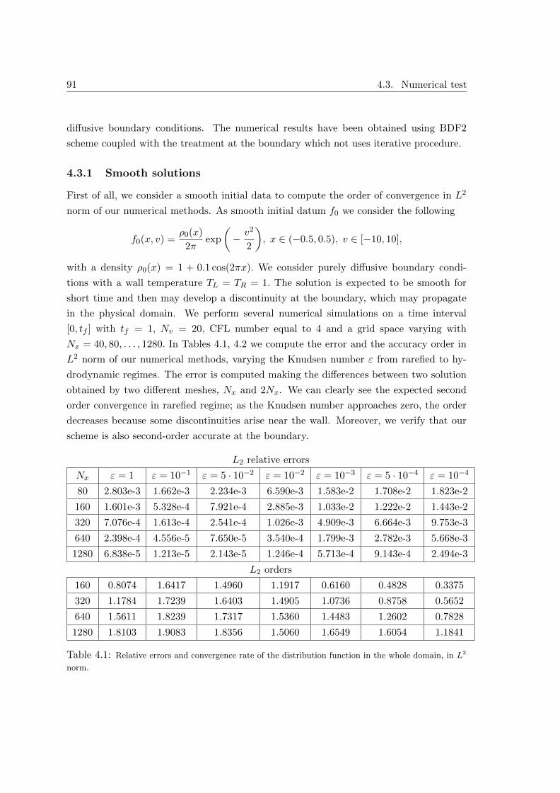
91 4.3. Numerical test
diffusive boundary conditions. The numerical results have been obtained using BDF2
scheme coupled with the treatment at the boundary which not uses iterative procedure.
4.3.1 Smooth solutions
First of all, we consider a smooth initial data to compute the order of convergence in L2
norm of our numerical methods. As smooth initial datum f0 we consider the following
f0(x, v) =ρ0(x)
2πexp
(− v2
2
), x ∈ (−0.5, 0.5), v ∈ [−10, 10],
with a density ρ0(x) = 1 + 0.1 cos(2πx). We consider purely diffusive boundary condi-
tions with a wall temperature TL = TR = 1. The solution is expected to be smooth for
short time and then may develop a discontinuity at the boundary, which may propagate
in the physical domain. We perform several numerical simulations on a time interval
[0, tf ] with tf = 1, Nv = 20, CFL number equal to 4 and a grid space varying with
Nx = 40, 80, . . . , 1280. In Tables 4.1, 4.2 we compute the error and the accuracy order in
L2 norm of our numerical methods, varying the Knudsen number ε from rarefied to hy-
drodynamic regimes. The error is computed making the differences between two solution
obtained by two different meshes, Nx and 2Nx. We can clearly see the expected second
order convergence in rarefied regime; as the Knudsen number approaches zero, the order
decreases because some discontinuities arise near the wall. Moreover, we verify that our
scheme is also second-order accurate at the boundary.
L2 relative errors
Nx ε = 1 ε = 10−1 ε = 5 · 10−2 ε = 10−2 ε = 10−3 ε = 5 · 10−4 ε = 10−4
80 2.803e-3 1.662e-3 2.234e-3 6.590e-3 1.583e-2 1.708e-2 1.823e-2
160 1.601e-3 5.328e-4 7.921e-4 2.885e-3 1.033e-2 1.222e-2 1.443e-2
320 7.076e-4 1.613e-4 2.541e-4 1.026e-3 4.909e-3 6.664e-3 9.753e-3
640 2.398e-4 4.556e-5 7.650e-5 3.540e-4 1.799e-3 2.782e-3 5.668e-3
1280 6.838e-5 1.213e-5 2.143e-5 1.246e-4 5.713e-4 9.143e-4 2.494e-3
L2 orders
160 0.8074 1.6417 1.4960 1.1917 0.6160 0.4828 0.3375
320 1.1784 1.7239 1.6403 1.4905 1.0736 0.8758 0.5652
640 1.5611 1.8239 1.7317 1.5360 1.4483 1.2602 0.7828
1280 1.8103 1.9083 1.8356 1.5060 1.6549 1.6054 1.1841
Table 4.1: Relative errors and convergence rate of the distribution function in the whole domain, in L2
norm.
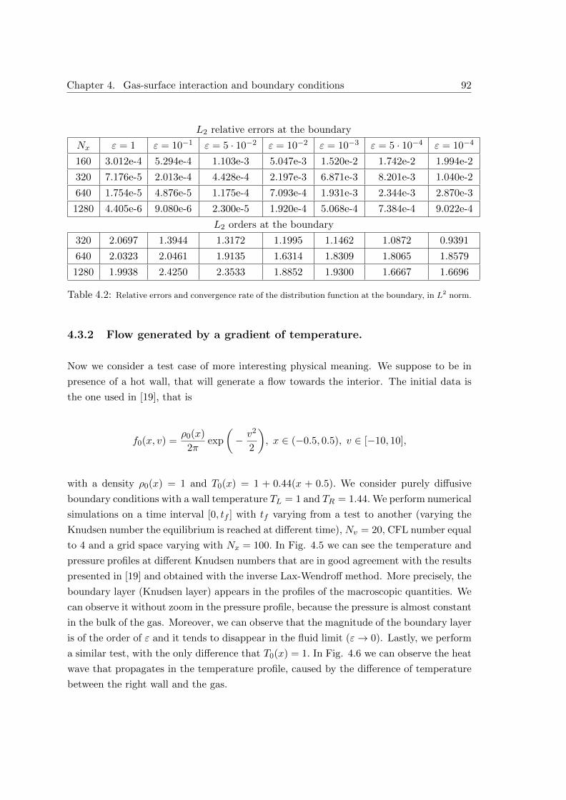
Chapter 4. Gas-surface interaction and boundary conditions 92
L2 relative errors at the boundary
Nx ε = 1 ε = 10−1 ε = 5 · 10−2 ε = 10−2 ε = 10−3 ε = 5 · 10−4 ε = 10−4
160 3.012e-4 5.294e-4 1.103e-3 5.047e-3 1.520e-2 1.742e-2 1.994e-2
320 7.176e-5 2.013e-4 4.428e-4 2.197e-3 6.871e-3 8.201e-3 1.040e-2
640 1.754e-5 4.876e-5 1.175e-4 7.093e-4 1.931e-3 2.344e-3 2.870e-3
1280 4.405e-6 9.080e-6 2.300e-5 1.920e-4 5.068e-4 7.384e-4 9.022e-4
L2 orders at the boundary
320 2.0697 1.3944 1.3172 1.1995 1.1462 1.0872 0.9391
640 2.0323 2.0461 1.9135 1.6314 1.8309 1.8065 1.8579
1280 1.9938 2.4250 2.3533 1.8852 1.9300 1.6667 1.6696
Table 4.2: Relative errors and convergence rate of the distribution function at the boundary, in L2 norm.
4.3.2 Flow generated by a gradient of temperature.
Now we consider a test case of more interesting physical meaning. We suppose to be in
presence of a hot wall, that will generate a flow towards the interior. The initial data is
the one used in [19], that is
f0(x, v) =ρ0(x)
2πexp
(− v2
2
), x ∈ (−0.5, 0.5), v ∈ [−10, 10],
with a density ρ0(x) = 1 and T0(x) = 1 + 0.44(x + 0.5). We consider purely diffusive
boundary conditions with a wall temperature TL = 1 and TR = 1.44.We perform numerical
simulations on a time interval [0, tf ] with tf varying from a test to another (varying the
Knudsen number the equilibrium is reached at different time), Nv = 20, CFL number equal
to 4 and a grid space varying with Nx = 100. In Fig. 4.5 we can see the temperature and
pressure profiles at different Knudsen numbers that are in good agreement with the results
presented in [19] and obtained with the inverse Lax-Wendroff method. More precisely, the
boundary layer (Knudsen layer) appears in the profiles of the macroscopic quantities. We
can observe it without zoom in the pressure profile, because the pressure is almost constant
in the bulk of the gas. Moreover, we can observe that the magnitude of the boundary layer
is of the order of ε and it tends to disappear in the fluid limit (ε→ 0). Lastly, we perform
a similar test, with the only difference that T0(x) = 1. In Fig. 4.6 we can observe the heat
wave that propagates in the temperature profile, caused by the difference of temperature
between the right wall and the gas.
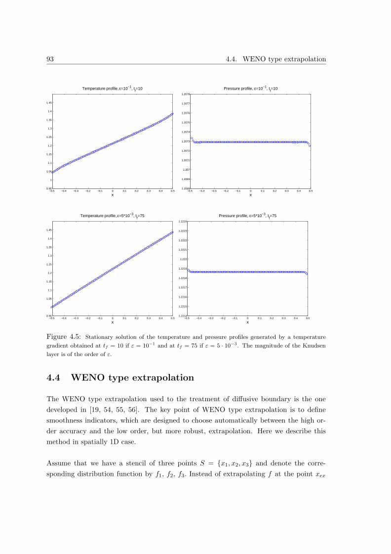
93 4.4. WENO type extrapolation
−0.5 −0.4 −0.3 −0.2 −0.1 0 0.1 0.2 0.3 0.4 0.50.95
1
1.05
1.1
1.15
1.2
1.25
1.3
1.35
1.4
1.45
Temperature profile, ε=10−1, tf=10
x−0.5 −0.4 −0.3 −0.2 −0.1 0 0.1 0.2 0.3 0.4 0.5
1.2068
1.2069
1.207
1.2071
1.2072
1.2073
1.2074
1.2075
1.2076
1.2077
1.2078
Pressure profile, ε=10−1, tf=10
x
−0.5 −0.4 −0.3 −0.2 −0.1 0 0.1 0.2 0.3 0.4 0.50.95
1
1.05
1.1
1.15
1.2
1.25
1.3
1.35
1.4
1.45
Temperature profile, ε=5*10−3, tf=75
x−0.5 −0.4 −0.3 −0.2 −0.1 0 0.1 0.2 0.3 0.4 0.5
1.2214
1.2215
1.2216
1.2217
1.2218
1.2219
1.222
1.2221
1.2222
1.2223
1.2224
Pressure profile, ε=5*10−3, tf=75
x
Figure 4.5: Stationary solution of the temperature and pressure profiles generated by a temperature
gradient obtained at tf = 10 if ε = 10−1 and at tf = 75 if ε = 5 · 10−3. The magnitude of the Knudsen
layer is of the order of ε.
4.4 WENO type extrapolation
The WENO type extrapolation used to the treatment of diffusive boundary is the one
developed in [19, 54, 55, 56]. The key point of WENO type extrapolation is to define
smoothness indicators, which are designed to choose automatically between the high or-
der accuracy and the low order, but more robust, extrapolation. Here we describe this
method in spatially 1D case.
Assume that we have a stencil of three points S = x1, x2, x3 and denote the corre-
sponding distribution function by f1, f2, f3. Instead of extrapolating f at the point xex
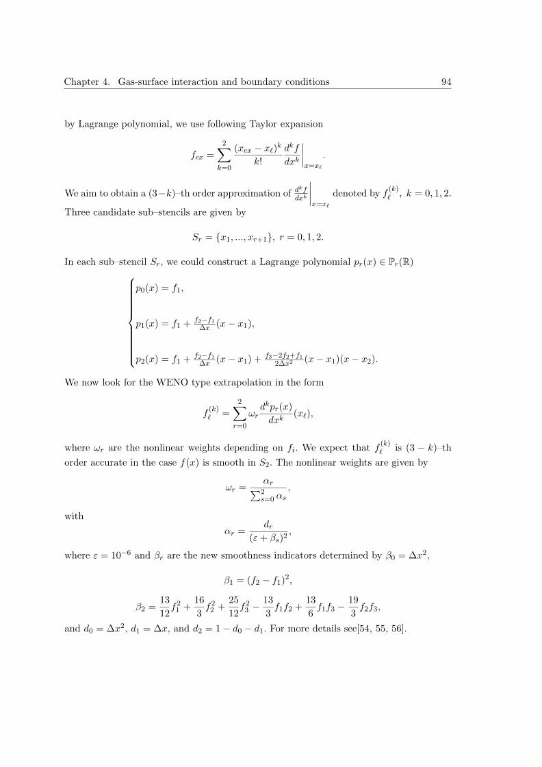
Chapter 4. Gas-surface interaction and boundary conditions 94
by Lagrange polynomial, we use following Taylor expansion
fex =2∑
k=0
(xex − x`)kk!
dkf
dxk
∣∣∣∣x=x`
.
We aim to obtain a (3−k)–th order approximation of dkfdxk
∣∣∣∣x=x`
denoted by f(k)` , k = 0, 1, 2.
Three candidate sub–stencils are given by
Sr = x1, ..., xr+1, r = 0, 1, 2.
In each sub–stencil Sr, we could construct a Lagrange polynomial pr(x) ∈ Pr(R)
p0(x) = f1,
p1(x) = f1 + f2−f1∆x (x− x1),
p2(x) = f1 + f2−f1∆x (x− x1) + f3−2f2+f1
2∆x2(x− x1)(x− x2).
We now look for the WENO type extrapolation in the form
f(k)` =
2∑
r=0
ωrdkpr(x)
dxk(x`),
where ωr are the nonlinear weights depending on fi. We expect that f(k)` is (3 − k)–th
order accurate in the case f(x) is smooth in S2. The nonlinear weights are given by
ωr =αr∑2s=0 αs
,
with
αr =dr
(ε+ βs)2,
where ε = 10−6 and βr are the new smoothness indicators determined by β0 = ∆x2,
β1 = (f2 − f1)2,
β2 =13
12f2
1 +16
3f2
2 +25
12f2
3 −13
3f1f2 +
13
6f1f3 −
19
3f2f3,
and d0 = ∆x2, d1 = ∆x, and d2 = 1− d0 − d1. For more details see[54, 55, 56].
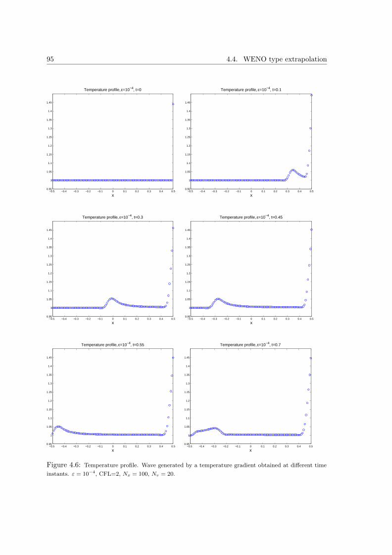
95 4.4. WENO type extrapolation
−0.5 −0.4 −0.3 −0.2 −0.1 0 0.1 0.2 0.3 0.4 0.50.95
1
1.05
1.1
1.15
1.2
1.25
1.3
1.35
1.4
1.45
Temperature profile, ε=10−4, t=0
x−0.5 −0.4 −0.3 −0.2 −0.1 0 0.1 0.2 0.3 0.4 0.5
0.95
1
1.05
1.1
1.15
1.2
1.25
1.3
1.35
1.4
1.45
Temperature profile, ε=10−4, t=0.1
x
−0.5 −0.4 −0.3 −0.2 −0.1 0 0.1 0.2 0.3 0.4 0.50.95
1
1.05
1.1
1.15
1.2
1.25
1.3
1.35
1.4
1.45
Temperature profile, ε=10−4, t=0.3
x−0.5 −0.4 −0.3 −0.2 −0.1 0 0.1 0.2 0.3 0.4 0.5
0.95
1
1.05
1.1
1.15
1.2
1.25
1.3
1.35
1.4
1.45
Temperature profile, ε=10−4, t=0.45
x
−0.5 −0.4 −0.3 −0.2 −0.1 0 0.1 0.2 0.3 0.4 0.50.95
1
1.05
1.1
1.15
1.2
1.25
1.3
1.35
1.4
1.45
Temperature profile, ε=10−4, t=0.55
x−0.5 −0.4 −0.3 −0.2 −0.1 0 0.1 0.2 0.3 0.4 0.5
0.95
1
1.05
1.1
1.15
1.2
1.25
1.3
1.35
1.4
1.45
Temperature profile, ε=10−4, t=0.7
x
Figure 4.6: Temperature profile. Wave generated by a temperature gradient obtained at different time
instants. ε = 10−4, CFL=2, Nx = 100, Nv = 20.

Chapter 4. Gas-surface interaction and boundary conditions 96
Chapter 5
BGK models for gas mixtures and
semi-Lagrangian approximation
Most of the BGK models have been considered in the case of a single species gas. This
seems an important limitation, recalling for example that the atmosphere must be at
least considered as a binary mixture of Oxygen and Nitrogen. Although the extension
of the Boltzmann equation to a mixture of gases has been well known for a long time,
this is not the case for the BGK equation. Considerable troubles are encountered if one
tries to extend the BGK philosophy, originally devised for a single species gas, to a gas
mixture [52, 21]. Indeed, one faces immediately very basic drawbacks such as loss of
positivity of temperature and breakdown of the indifferentiability principle. An accurate
and detailed discussion on the subject may be found in [3], where the authors propose a
simple and very interesting consistent BGK-type model for gas mixtures which overcomes
all previous difficulties. In this Chapter kinetic and BGK equations for both inert and
reactive gas mixtures are presented. Moreover, numerical results, obtained by means of
the semi-Lagrangian schemes proposed, are shown.
5.1 Boltzmann equation for inert gas mixtures
We consider now a gas mixture of L different species Gs, s = 1, · · · , L. The kinetic de-
scription is given by L Boltzmann equations for distribution functions fs(t, x, v), (t, x, v) ∈R+ × R3 × R3
∂fs
∂t+ v · ∇xfs = Qs, s = 1, · · · , L, (5.1)
97
Chapter 5. BGK models for gas mixtures and semi-Lagrangian approximation 98
where
Qs =L∑
r=0
Qsr(fs, f r), s = 1, · · · , L,
and
Qsr(fs, f r) =
∫
R3
∫
S2Bsr(v, w,Ω)[f s(v′)f r(w′)− fs(v)f r(w)] dΩ dw
is the usual scattering collision operator for the binary (s, r) interaction.
We introduce notations for macroscopic quantities that will be used later on: ms is the
molecular masses, ns the number density, ρs the density, us the average velocity, T s the
temperature of species s. One has:
ns =
∫
R3
fs dv, ρs = msns
us =1
ns
∫
R3
vfs dv
nsKBTs =
1
3ms
∫
R3
(v − us)2fs dv.
Then we also have global quantities for the mixture, the number density n, the total
density ρ, the mean velocity u, scalar pressure p or temperature T, which are expressed
in terms of single component parameters by
n =L∑
s=1
ns, ρ =L∑
s=1
ρs =L∑
s=1
msns,
u =1
ρ
L∑
s=1
msnsus,
p = nKBT =
L∑
s=1
nsKBTs +
1
3
L∑
s=1
msns(us − u)2.
Of course the Boltzmann equation for mixture has to satisfy the indifferentiability princi-
ple. It states that, when all the masses ms and cross-sections Bsr are identical, the total
distribution function f =∑L
s=1 fs obeys the single species Boltzmann equation. Notice
also that the macroscopic quantities associated to f are n, u and T in this case.
For multispecies gases, we have to keep in mind that for each species mass, momentum
and energy are not necessarily conserved. If we suppose that there is no chemical reaction
between the species, the mass of each species is conserved∫
R3
Qs dv = 0, s = 1, · · · , L (5.2)
99 5.1. Boltzmann equation for inert gas mixtures
Each species may nevertheless exchange momentum and energy with the others, so the
species momentum and energy cannot be conserved in general. Such rates can be made
explicit for Maxwellian molecules [13]. In detail, the exchange relations can be computed
and one obtains [3, 22]:
∫
R3
msvQs dv =
L∑
r=1
νsr1 µsrnsnr(ur − us), (5.3)
∫
R3
ms
2v2Qs dv =
L∑
r=1
νsr1
2µsr
ms +mrnsnr
[3
2KB(T r−T s)+1
2(mrur+msus)·(ur−us)
], (5.4)
where µsr is the reduced mass
µsr =msmr
ms +mr,
and νsrk (g) = νrsk (g) are the microscopic collision frequencies
νsrk (g) = νrsk (g) = 2πg
∫ π
0σsr(g, χ)(1− cosχ)k sinχdχ, k = 0, 1, (5.5)
with νsrk ≤ 2νsr0 and σ stands for differential cross section and g is the relative speed.
Actually, under the hypothesis of Maxwellian molecules (σsr(g, χ) ∝ 1/g) the microscopic
collision frequencies are constant with respect to the relative speed g. Of course
L∑
s=1
∫
R3
msv Qs dv = 0 andL∑
s=1
∫
R3
1
2msv2Qs dv = 0
that is, the momentum and the energy of the global mixture are conserved. Thus, in a
mixture without chemical reaction there are L+4 collision invariants, relevant to the mass
of each species, to the total momentum and total kinetic energy.
The equilibrium in the mixture is obtained when all Qs = 0. Then Qsr = 0. It can
be proved that if for two species s and r Qsr = Qrs = 0 then fs and f r are Maxwellians
with common velocity and temperature. The conclusion is that at global equilibrium, all
distributions are Maxwellians of the form
fs = ns(
ms
2πKBT
)3/2
exp
(− ms|v − u|2
2KBT
), (5.6)
with common velocity u and temperature T.
In a spatially uniform state (∇xf = 0), the H-theorem can be proved choosing the following
H-function [3]
H =L∑
s=1
∫
R3
f s ln(fs) dv, (5.7)
Chapter 5. BGK models for gas mixtures and semi-Lagrangian approximation 100
and, in the case of mixture, the entropy inequality is
L∑
s=1
∫
R3
Qs ln(fs) dv ≤ 0.
5.2 BGK models for inert gas mixtures
After the introduction of the BGK model for one-species gas, many attempts have been
made to extend the BGK model to gas mixture. The trivial extension
∂fs
∂t+ v · ∇xfs = νs(M s − fs), s = 1, · · · , L
where νs is the species collision frequencies and M s is the local Maxwellian with density,
momentum and temperature of the species s is not consistent because it does not reproduce
equilibrium conditions us = u and T s = T ∀s.Among the pioneering BGK models for mixtures we can cite [26, 52, 21]. The models
presented in [26, 52] have an important drawback: when all species are identical one
does not recover the BGK equation for a single gas, that is, they do not satisfy the
indifferentiability principle. In [21] a different model overcoming this drawback is proposed,
but positivity is lost. Here we present two consistent BGK models for inert mixtures which
overcome all previous difficulties.
5.2.1 The BGK model of Andries, Aoki and Perthame
The first consistent BGK model for inert mixtures, satisfying the main properties of the
Boltzmann equation for mixtures, such as positivity, indifferentiability principle and en-
tropy inequality, was introduced in [3]. The key idea is that instead of approximating
each binary collision operator (between specie s and r) by a BGK-type equation, only one
global operator is introduced (i.e., taking into account all the species r) for each species
s. The model is built as follows. The relaxation occurs toward a Maxwellian distribution
Ms, i.e.,∂fs
∂t+ v · ∇xf s = QsBGK = νs(Ms − fs), s = 1, · · · , L, (5.8)
where fs is the distribution function of the species s, Ms is an auxiliary local Maxwellian
depending on velocity vector variable v, molecular masses ms, Boltzmann constant KB
and disposable parameters ns, us, Ts
Ms = ns
(ms
2πKBTs
)3/2
exp
(− ms
2KBTs(v − us)2
), s = 1, · · · , L. (5.9)
101 5.2. BGK models for inert gas mixtures
(Note the subscript s, while actual macroscopic fields have a superscript s).
At last, νs represents the inverse of the sth relaxation time, possibly depending on macro-
scopic fields, but independent of v. The authors in [3] emphasize that the choice of νs is
crucial. In particular the model is well defined with the total collision frequency
νs =L∑
r=1
νsr0 nr. (5.10)
With this choice of νs it can be proved [3] that the positivity of the temperature is en-
sured. The above auxiliary fields ns, us, Ts are determined from the corresponding actual
moments of the distribution functions fs (namely number density ns, mass velocity us
and temperature T s of each component) by requiring that the BGK model prescribes the
same exchange rates by collisions of the Boltzmann level given in (5.3)-(5.4). By (5.2) of
course ns = ns ∀s, since∫R3 Q
sBGK = ns − ns must be zero. Following [3], we now impose
that the Boltzmann equation (5.1) and its approximate model (5.8) prescribe the same
exchange rates (5.3) and (5.4), that is:
∫
R3
msvQsBGK dv =
∫
R3
msvQs dv
or equivalently
msnsus −msnsus =L∑
r=1
νsr1 µsrnsnr(ur − us)
and ∫
R3
1
2msv2QsBGK dv =
∫
R3
1
2msv2Qs dv
or equivalently
νs
[ns
3
2KBTs − ns
3
2KBT
s + ns1
2msu2
s − ns1
2ms(us)2
]=
=
L∑
r=1
νsr1
2µsr
ms +mrnsnr
[3
2KB(T r − T s) +
1
2(mrur +msus) · (ur − us)
].
Upon introducing the auxiliary symmetric matrices
ξsr = ξrs = νsr1 µsrnsnr − δsr
L∑
l=1
νsl1 µslnsnr,
γsr = γrs = 3KBνsr1
µsr
ms +mrnsnr − δsr3KB
L∑
l=1
νsl1
µsl
ms +mlnsnl,
Chapter 5. BGK models for gas mixtures and semi-Lagrangian approximation 102
where δsr denotes the usual Kronecker symbol, the parameters determining all attracting
Maxwellians Ms read explicitly as
us =1
msns
[msnsus +
1
vs
L∑
r=1
ξsrur], (5.11)
Ts =2
3nsKB
[ns
3
2KBT
s − 1
2ms[ns(us)
2 − ns(us)2] +1
νs
L∑
r=1
γsrT r+
+1
νs
4∑
r=1
νsr1
µsr
ms +mrnsnr(msus +mrur)(ur − us)
]. (5.12)
Under the hypothesis (5.10) Andries, Aoki and Perthame proved in [3] that the temper-
atures (5.12) are positive. The above scheme guarantees that the BGK approximation
fulfills the main features of the actual collision operator. Obviously the conservation
equations are recovered by construction. Moreover, the main properties, such us indiffer-
entiability principle, H-theorem and entropy inequality are recovered. The H-theorem can
be proved using the same H-function (5.7) of the Boltzmann level [3]. Indeed,
∂
∂tH =
∂
∂t
L∑
s=1
∫
R3
fs ln(f s) dv ≤ 0.
As a consequence, in the time evolution the BGK model pushes the distribution function
towards the local equilibrium M s, where M s is the L+4-parameter family of Maxwellians
distributions given in (5.6) with global mass velocity u and temperature T.
5.2.2 A new BGK model for inert mixtures
In the previous model for inert mixtures, have been introduced 4L auxiliary parameters,
namely us and T s, s = 1, · · · , L in order to recover the same exchange rates of the
Boltzmann level and the correct conservation equations. Now we introduce a new BGK
model which does not reproduce the species exchange rates of the Boltzmann level, but
only the conservation of total momentum and kinetic energy. In this way, one obtains a
BGK model of the form
∂fs
∂t+ v · ∇xf s = QsBGK = νs(Ms − fs), s = 1, · · · , L, (5.13)
where now the attractors Ms are fictitious Maxwellians
Ms = ns(
ms
2πKBT
)3/2
exp
(− ms
2KBT(v − u)2
), s = 1, · · · , L, (5.14)
103 5.2. BGK models for inert gas mixtures
defined in terms of L+ 4 (instead of 5L) auxiliary parameters ns, s = 1, · · · , L, u, and T .
The main difference with the previous BGK model is that now the attractor Ms have com-
mon fictitious velocities and temperature u and T . In other words, the model pushes the
gas towards a full, instead of partial, equilibrium. Once again, the auxiliary macroscopic
fields depend on the actual macroscopic fields of fs and are determined in such a way to
satisfy the conservation of mass, momentum and energy. Of course ns = ns since we are
considering inert mixtures. Imposing the total conservation of momentum and energy we
obtainL∑
s=1
∫
R3
msvQsBGK dv = 0 (5.15)
or equivalentlyL∑
s=1
νsmsns(u− us) = 0
and for the energyL∑
s=1
∫
R3
1
2msv2QsBGK dv = 0 (5.16)
or equivalently
L∑
s=1
νs
[1
2msnsu2 +
3
2nsKBT −
1
2msns(us)2 − 3
2nsKBT
s
]= 0.
Therefore, the parameters determining the Maxwellians (5.14) read explicitly as
u =
∑Ls=1 νsm
snsus∑L
s=1 νsmsns
, (5.17)
T =
∑Ls=1 νsn
s[
12m
s((us)2 − u2) + 32KBT
s]
32KB
∑Ls=1 νsn
s. (5.18)
As the BGK model of Andries, Aoki and Perthame, the above scheme satisfies the main
properties, such us positivity, indifferentiability principle; also the H-theorem and entropy
inequality are recovered.
As regards positivity, we have to prove that T in (5.18) is positive.
Theorem 5.2.1. The global temperature T (5.18) is positive.
Proof. We observe that T is positive is and only if
( L∑
s=1
αsus
)2
≤L∑
s=1
αs|us|2 (5.19)
Chapter 5. BGK models for gas mixtures and semi-Lagrangian approximation 104
where∑L
s=1 αs = 1. Indeed,
T > 0⇔L∑
s=1
νsns[ms((us)2 − u2) + 3KBT
s] > 0⇔
⇔L∑
s=1
νsnsmsu2 <
L∑
s=1
νsns[ms(us)2 + 3KBT
s]⇔
⇔ u2 <
L∑
s=1
αs
[(us)2 + 3KB
T s
ms
],
where
αs =νsnsms
∑Ls=1 ν
snsms.
Expression (5.19) follows observing that u =∑L
s=1 αsus.
Now we prove by induction that (∑L
s=1 αsus)2 ≤ ∑L
s=1 αs|us|2, with us = (usx, usy, u
sz) ∈
R3,∑L
s=1 αs = 1, αs ≥ 0 ∀s.
Case L = 2.
(α1u1 + α2u
2)2 = (α1u1x + α2u
2x)2 + (α1u
1y + α2u
2y)
2 + (α1u1z + α2u
2z)
2 =
= α21
[(u1x)2 + (u1
y)2 + (u1
z)2]
+ α22
[(u2x)2 + (u2
y)2 + (u2
z)2]+
+2α1α2u1xu
2x + 2α1α2u
1yu
2y + 2α1α2u
1zu
2z.
(α1u1 + α2u
2)2 − α1|u1|2 − α2|u2|2 =
= (α21 − α1)
[(u1x)2 + (u1
y)2 + (u1
z)2]
+ (α22 − α2)
[(u2x)2 + (u2
y)2 + (u2
z)2]+
+2α1α2u1xu
2x + 2α1α2u
1yu
2y + 2α1α2u
1zu
2z =
= −α1α2
[(u1x)2 + (u1
y)2 + (u1
z)2 + (u2
x)2 + (u2y)
2 + (u2z)
2+
−2(u1x)2(u2
x)2 − 2(u1y)
2(u2y)
2 − 2(u1z)
2(u2z)
2]
=
= −α1α2
[(u1x − u2
x)2 + (u1y − u2
y)2 + (u1
z − u2z)
2]
= −α1α2|u1 − u2|2 ≤ 0.
105 5.2. BGK models for inert gas mixtures
Finally, supposed that the property holds for L− 1, now we prove it for L.
L∑
s=1
αsus = (1− αL)
L−1∑
s=1
βsus + αLu
L = γ1ω1 + γ2ω2,
where
βs =αs
1− αL,
L−1∑
s=1
βs =
∑L−1s=1 αs
1− αL= 1,
γ1 = 1− αL, γ2 = αL, ω1 =
L−1∑
s=1
βsus, ω2 = uL.
Then, we obtain
(L∑
s=1
αsus)2 ≤ γ1|ω1|2 + γ2|ω2|2 = (1− αL)(
L−1∑
s=1
βsus)2 + αL|uL|2 ≤
≤ (1− αL)L−1∑
s=1
βs|us|2 + αL|uL|2 =L∑
s=1
αs|us|2.
The H-theorem can be easily proved.
Theorem 5.2.2. Let
H =L∑
s=1
∫
R3
f s ln(fs) dv.
Then H ≤ 0, and H = 0 if and only if f s = Ms
Proof.
H =L∑
s=1
∫
R3
˜QsBGK ln(fs) dv =
=L∑
s=1
∫
R3
νs(Ms − fs) ln(fs) dv.
We observe that from conservations (5.15) and (5.16) follows that
L∑
s=1
∫
R3
QsBGK ln(M s) dv = 0.
Then we can write
H =L∑
s=1
∫
R3
QsBGK [ln(fs)− ln(M s)] dv =L∑
s=1
∫
R3
(M s − fs) ln
(fs
M s
)dv =
Chapter 5. BGK models for gas mixtures and semi-Lagrangian approximation 106
=L∑
s=1
νs
∫
R3
M s
(1− fs
M s
)ln
(fs
M s
)dv ≤ 0.
The last inequality holds because the function (x − 1) lnx is always positive except in
x = 1 where it vanishes.
As a consequence, the time evolution pushes the distribution function towards the local
equilibrium M s, where M s is the Maxwellian distribution
M s = ns(
ms
2πKBT
)3/2
exp
(− ms
2KBT(v − u)2
), s = 1, · · · , L,
with global mass velocity u and temperature T.
5.3 BGK model for reactive mixtures
Now we introduce an extension of the previous BGK model (5.8), due to Groppi and Spiga
[25], to the much more complicated problems, significant for applications, in which gas
components may undergo chemical reactions.
The main difference with the inert BGK model is that now also exchange of mass and of
energy of chemical link have to be considered. In particular, the authors in [25] deal with
a four species gas mixture and with the reversible chemical reaction
A1 +A2 A3 +A4. (5.20)
Molecules As are endowed with an energy of chemical bond Es and may also interact with
any, different or equal, species r = 1, · · · , 4 by elastic scattering.
The system of Boltzmann equations describing these processes has been derived and inves-
tigate in [47]. Here we just recall that there exist seven independent collision invariants,
and they may be chosen as three combinations of number densities ns + nr, for instance
(s, r) = (1, 3), (1, 4), (2, 4), (relevant to the balance between reactants and products), the
global mass velocity and the internal (kinetic plus chemical) energy. Consequently, we get
seven exact, non-closed, macroscopic conservation equations. Correspondingly, we have
now a seven-parameter family of Maxwellians
M s(v) = ns(
ms
2πKBT
)3/2
exp
(− ms
2KBT(v − u)2
),
as collision equilibria, with equilibrium densities bound together by the well known mass
action law of chemistry
n1n2
n3n4=
(µ12
µ34
)3/2
exp
(∆E
KBT
), (5.21)
107 5.3. BGK model for reactive mixtures
where ∆E is the energy threshold ∆E = −∑4s=1 λ
sEs > 0 (with λ1 = λ2 = −λ3 = −λ4 =
1) to be overcome in the endothermic reaction, conventionally assumed to be the one from
the left to the right in (5.20). A strict entropy inequality for relaxation to equilibrium has
also been established in terms of the H functional [47]
H =4∑
s=1
∫
R3
fs ln(fs/(ms)3). dv (5.22)
5.3.1 The BGK model of Groppi and Spiga
The main structure of this BGK model for reactive mixture is similar to (5.8), (5.9) and
(5.10). The substantial differences consist in expression (5.11) and (5.12), since now also
the chemical exchange rates have to be considered. As a consequence, here the single
number densities ns are not conserved quantities, and therefore also number density of
the attracting sth Maxwellian is different from that of the actual distribution function. In
detail, under the assumption of tempered reaction regime, the parameters determining all
Maxwellian Ms read explicitly as [25]
ns = ns +λs
νsS, (5.23)
msnsus = msnsus +1
νs
4∑
r=1
ξsrur +λs
νsmsuS, (5.24)
ns3
2KBTs = ns
3
2KBT
s − 1
2ms[nsu
2s − ns(us)2] +
1
νs
4∑
r=1
γsrT r+
1
νs
4∑
r=1
νsr1
µsr
ms +mrnsnr(msus +mrur) · (ur − us)+
+λs
νsS
[M −ms
MKBT
(∆E
KBT
)3/2 e−∆E/KBT
Γ(32 ,
∆EKBT
)
+1
2msns +
3
2KBT −
1− λs2
M −ms
M∆E
], (5.25)
where
S = ν3412
2√2
Γ
(3
2,
∆E
KBT
)[n3n4
(m1m2
m3m4
)3/2
e∆E/KBT − n1n2
], (5.26)
ν3412(g) = 2πg
∫ π
0σ34
12(g, χ) sinχdχ,
Chapter 5. BGK models for gas mixtures and semi-Lagrangian approximation 108
Γ denotes an incomplete Gamma function, M = m1 +m2 = m3 +m4.
This BGK model is a robust approximation of the Boltzmann-type kinetic equation de-
scribing the reaction mixtures, since it correctly reproduces equilibria (including mass
action low) and conservation equations. As regards the H-theorem, an analytical proof
using the H function (5.22) is still lacking in [25], due to the considerable difficulties in-
troduced by the chemical reaction. However, numerical results show the expected trend
of the H-functional.
5.4 Numerical treatment
The numerical methods presented in Chapter 3 have been successfully extended to the
case of inert and reactive mixtures. We have considered problems 3D in velocity (here
we denote the full velocity vector v = (v1, v2, v3)), 1D in space, in slab geometry. The
starting point is the Chu reduction [15] introduced in Section 1.4, which, under suitable
symmetry assumption, allows to transform a 3D equation (in velocity) in a system of two
equations 1D (in velocity).
For the sake of simplicity, we fix L = 4, and discretize the BGK model of Andries, Aoki and
Perthame; the discretizazion of the other BGK models described in Section 5.2.2 is similar.
5.4.1 First order SL scheme for the AAP BGK model
Let us introduce the new unknowns
gs1(t, x, v) =
∫
R2
fs(t, x, v) dv2dv3, gs2(t, x, v) =
∫
R2
(v22 + v2
3)fs(t, x, v) dv2dv3, (5.27)
each depending only on one space and one velocity variable v = v1. Multiplication of (5.8)
by 1 and (v22 + v2
3) and integration with respect to (v2, v3) ∈ R2 yields then the following
system of BGK equations for the unknown vector gs = (gs1, gs2), coupled with initial con-
ditions
∂gsi∂t
+ v∂gsi∂x
= νs(Ms,i − gsi ), (t, x, v) ∈ R+ × R× R,
gsi (0, x, v) = gsi,0(x, v), s = 1, ..., 4, i = 1, 2.
(5.28)
The BGK system (5.28) describes a relaxation process towards the vector Maxwellians
109 5.4. Numerical treatment
(Ms,1,Ms,2), which is obtained by Chu transform of (5.9) and has the form
(Ms,1,Ms,2) =
(Ms,
2KBTsms
Ms
),
where
Ms = ns(
ms
2πKBTs
)1/2
exp
(− ms
2KBTs(v − us)2
), s = 1, · · · , 4.
To determine the auxiliary parameters us and Ts we have to solve (5.11) and (5.12). Rela-
tions (5.11) and (5.12) involve fundamental macroscopic moments of distribution functions
fs, ns, us and T s, which are given in terms of gs1 and gs2 as
ns =
∫
Rgs1 dv, us =
1
ns
∫
Rvgs1 dv,
3KBTs
ms=
1
ns
[ ∫
R(v − us)2gs1 dv +
∫
Rgs2 dv
].
Now we apply the first order SL scheme to the system (5.28). In this case it reads as
gs,n+11,ij = gs,n1,ij + ∆tνn+1
s,ij (Mn+1s,1,ij − g
s,n+11,ij ), s = 1, ..., 4,
gs,n+12,ij = gs,n2,ij + ∆tνn+1
s,ij (Mn+1s,2,ij − g
s,n+12,ij ), s = 1, ..., 4,
(5.29)
where gs,n1,ij = gs1(tn, xi − vj∆t, vj) and gs,n2,ij = gs2(tn, xi − vj∆t, vj). The main drawback is
how to solve the implicit equations in (5.29), where the Maxwellians now depend on the
auxiliary fields.
By integrating over v the first equation of (5.29) for s = 1, · · · , 4 we obtain ns,n+1 = ns,n,
and then the collision frequencies νs, at time tn+1 can be evaluated.
The first task is to compute the fictitious mean velocities un+1s . To this end we recall
that
us =1
ns
∫
Rvgs1 dv,
us =1
msns
[msnsus +
1
νs
L∑
r=1
ξsrur].
Chapter 5. BGK models for gas mixtures and semi-Lagrangian approximation 110
Thus, if we multiply by v and then integrate on v the first equation of (5.29) for s = 1, ..., 4
we obtain (omitting the indexes relevant to the discretization)
nsus = nsus + ∆t νs(nsus − nsus), s = 1, · · · , 4, (5.30)
but, since ns,n+1 = ns,n, one obtains
us = us + ∆t νs(us − us), s = 1, · · · , 4, (5.31)
then using (5.11) one has
us = us + ∆t νs
(1
msnsνs
4∑
r=1
ξsrur), s = 1, · · · , 4, (5.32)
from which
(ξ11 − m1n1
∆t
)u1 + ξ12u2 + ξ13u3 + ξ14u4 = −m
1n1
∆tu1
ξ21u1 +
(ξ22 − m2n2
∆t
)u2 + ξ23u3 + ξ24u4 = −m
2n2
∆tu2
ξ31u1 + ξ32u2 +
(ξ33 − m3n3
∆t
)u3 + ξ34u4 = −m
3n3
∆tu3
ξ41u1 + ξ42u2 + ξ43u3 +
(ξ44 − m4n4
∆t
)u4 = −m
4n4
∆tu4
(5.33)
Thus we have to solve the system Au = b, where
A = ξ − 1
∆tdiag(m. ∗ n)
b = − 1
∆t(m. ∗ n. ∗ u)
where, in general, the notation a stands for (a1, a2, a3, a4)T, and a.∗b = (a1b1, a2b2, a3b3, a4b4)T.
111 5.4. Numerical treatment
Known the actual mean velocities, by (5.11) we are able to update the fictitious mean ve-
locities at time tn+1.
Now we have to compute the fictitious temperatures Tn+1s . To this end we recall that
3KBTs
ms=
1
ns
[ ∫
R(v − us)2gs1 dv +
∫
Rgs2 dv
], (5.34)
Ts =2
3nsKB
[ns
3
2KBT
s − 1
2msns[(us)
2 − (us)2] +1
νs
L∑
r=1
γsrT r+
+1
νs
4∑
r=1
νsr1
µsr
ms +mrnsnr(msus +mrur)(ur − us)
].
Thus, computing the species temperatures at time tn+1 by using (5.34) and replacing the
marginal distribution function g1 and g2 by their expression in (5.29) one obtains:
3nsKBTs
ms=
3nsKBTs
ms+∆tνs
(ns(us−us)2 +
3nsKBTsms
− 3nsKBTs
ms
)s = 1, ...4 (5.35)
T s −∆tνs(Ts − T s) = T s + ∆tνsms
3KB(us − us)2 s = 1, ...4 (5.36)
We denote
αs =ms
3KB(us − us)2
βs =ms
3KB[(us)
2 − (us)2]
γs =2
3KB
1
νs
4∑
r=1
νsr1
µsr
ms +mrnr(msus +mrur)(ur − us)
thus (5.36) becomes
T s − 2∆t
3nsKB
4∑
r=1
γsrT r = T s + ∆tνs(αs − βs + γs) s = 1, ...4 (5.37)
Chapter 5. BGK models for gas mixtures and semi-Lagrangian approximation 112
Thus we have to solve the system Au = b, where
A = γ − 3KB
2∆tdiag(n)
br = −3KBnr
2∆t
(T r + ∆tνr(αr − βr + γr)
)r = 1, ...4.
Once the actual temperatures are known, by (5.12) we are able to update the fictitious
temperatures at time tn+1.
In such a way we solve the implicit step. In analogous way it is possible to treat the other
BGK model (5.13) for inert mixtures with relations (5.17) and (5.18).
The extension to higher order schemes, once how to solve the implicit step is clear, is an
easy application of the schemes presented in Chapter 3. Numerical results in Section 5.5
are performed using the BDF2 scheme.
5.4.2 Sketch of the first order SL scheme for the reactive BGK model
The structure of the scheme is the same of the inert case. The solution of the BGK models
for reacting mixtures described in Section 5.3.1 leads to additional drawbacks, since we
have also auxiliary number densities ns, given in terms of the actual macroscopic fields
in equation (5.23), and the computation of the auxiliary fields now requires the solution
of a transcendental system of equations at each time step and at each spatial node, due
to the exponential term relevant to the mass action law (5.21), appearing in the term
S in the equations (5.23)-(5.26). Moreover, we do not get three uncoupled linear 4 × 4
systems, one for densities, one for the velocities and one for the temperatures, as in the
inert case. Indeed, each equation depends on all the twelve actual fields, since all of them
involve the term (5.26). As a consequence, the equations do not decouple, and we have a
12× 12 non linear system. Solve this non linear system by Newton method is prohibitive,
owing to the very complex expressions of the auxiliary fields (5.23), (5.24) and (5.25). To
overcome these difficulties we adopted an iterative procedure, similar to the one used for
the treatment of the diffusive boundary conditions in Chapter 4. At the step k = 0, we
suppose to have
gs,n+1,0
1,ij = gs,n1,ij
gs,n+1,02,ij = gs,n2,ij .
(5.38)
113 5.5. Numerical results
With this first approximation of gs,n+11,ij and gs,n+1
2,ij we compute a first approximation of
the actual fields and therefore of the auxiliary fields at time tn+1. Then we iterate the
procedure
gs,n+1,k
1,ij = gs,n1,ij + ∆tνs,n+1,k−1ij (M s,n+1,k−1
1,ij − gs,n+1,k−11,ij )
gs,n+1,k2,ij = gs,n2,ij + ∆tνs,n+1,k−1
ij (M s,n+1,k−12,ij − gs,n+1,k−1
2,ij ),(5.39)
until convergence. Fixed a tolerance tol, we stop the iterations when the 2-norm of the
difference of two consecutive iterates is smaller than tol for each marginal distribution
function gs1, gs2, s = 1, ..., 4. The number of iterates depends on ε/∆t. It increases as
ε → 0, and decreases as ∆t → 0. Thus, if we do not use very large CFL number we can
simulate fluid regime with a reasonable number of iterations without affecting the compu-
tational cost.
In a straightforward way we can extend these numerical scheme to high order schemes.
Numerical results are performed using the BDF2 scheme.
5.5 Numerical results
We have used the numerical test proposed in [1]. We consider a mixture of four monoatomic
gases with the following values of the molecular masses:
m1 = 58.5, m2 = 18, m3 = 40, m4 = 36.5.
We present some results for the following Riemann problem for both reactive and non-
reactive cases. The collision frequencies for elastic scattering are the same used in [1]:
ν110 = 500, ν12
0 = 600, ν130 = 200, ν14
0 = 700,
ν220 = 400, ν23
0 = 500, ν240 = 800,
ν330 = 400, ν34
0 = 300,
ν440 = 600,
with νsr0 = νrs0 and νsr1 = νsr0 for s, r = 1, ..., 4. The above frequencies will be multiplied
by a factor 1/ε in the numerical experiments, where ε is the Knudsen number, to simulate
by varying ε both rarefied and fluid regimes. The chemical collision frequency is ν3412 = 0
in the non-reactive case, whereas we set ν3412 = 100 in the reactive case. The initial data
Chapter 5. BGK models for gas mixtures and semi-Lagrangian approximation 114
are chosen as Maxwellians reproducing the following macroscopic fields:
(ρ0, u0, p0) =
(1, 0, 5/3), x < 0.5,
(1/8, 0, 1/6), x > 0.5,
(ρ01, ρ02, ρ03, ρ04) =
(1/10, 2/10, 3/10, 4/10), x < 0.5,
(1/80, 2/80, 3/80, 4/80), x > 0.5,(5.40)
u0i = 0, i = 1, ..., 4.
The presented results are obtained using BDF2 scheme, the best performing due to the
low number of interpolation required. In Figure 5.1 we present the result obtained in the
inert case. In this case, we set Nv = 30, Nx = 200, CFL = 2. In Figure 5.1 we compare
the result obtained with the two BGK models for inert case presented in subsections
5.2.1 and 5.2.2, respectively. The results are in good agreement with the ones present in
[1]. We can observe that at the final time tf = 0.2, for ε = 10−1 that implies in our case
νs ≈ 10−2, left column in Fig. 5.1, the equilibrium is not yet reached and species velocities
and temperatures are not yet relaxed to common values. Instead, we can observe that for
ε = 10−2 (νs ≈ 10−3, right column in Fig. 5.1) at the same final time we are closer to
the equilibrium, namely species velocities and temperatures almost overlap and give the
mean velocity and temperature of the mixture. In Fig. 5.2 the differences between the
mean velocity and temperature of the mixture and the species velocities and temperatures
are plotted. We can observe that the differences are smaller for the BGK model (5.13),
with respect to the ones obtained by the BGK model of Andries, Aoki and Perthame.
This is due to the fact that the BGK model (5.13) relaxes towards the attractors (5.14),
characterized by the presence of a common velocity and temperature. Instead the BGK
model of Andries, Aoki and Perthame relaxes towards attractors with different velocities
and temperatures, then species velocities and temperature equalize later.
Fig. 5.3, 5.4, 5.5 and 5.6 are relevant to the case of reactive mixture. We use a energy
threshold ∆E = 500. The results are relevant to the BGK model described in subsection
5.3.1. We can observe the variation of the number densities (Fig. 5.5) for different values of
ε. The density of the mixture is conserved, whereas the species densities are not, according
to conservations. The variations of the profiles for different values ∆E are shown in Fig.
5.7 and 5.8. In Figure 5.7 we report the global density ρ and densities ρ1 and ρ3 at time
t = 0.2 for non reactive e reactive case with ∆E = 0, 500, 1000. The global moments of
the inert mixture overlap the profiles obtained for ∆E = 0, whereas this is not the case for
the single components of the gas. The higher ∆E, the greater the variations with respect
to the inert case. The results obtained are in good agreement with those obtained in [1]
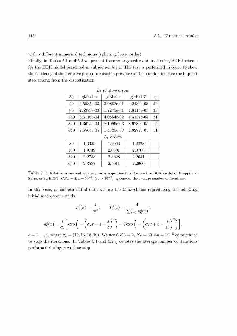
115 5.5. Numerical results
with a different numerical technique (splitting, lower order).
Finally, in Tables 5.1 and 5.2 we present the accuracy order obtained using BDF2 scheme
for the BGK model presented in subsection 5.3.1. The test is performed in order to show
the efficiency of the iterative procedure used in presence of the reaction to solve the implicit
step arising from the discretization.
L1 relative errors
Nx global n global u global T η
40 6.5535e-03 3.9862e-01 4.2436e-03 54
80 2.5973e-03 1.7275e-01 1.8118e-03 33
160 6.6116e-04 4.0854e-02 4.3127e-04 21
320 1.3625e-04 8.1096e-03 8.9780e-05 14
640 2.6564e-05 1.4325e-03 1.8282e-05 11
L1 orders
80 1.3353 1.2063 1.2278
160 1.9739 2.0801 2.0708
320 2.2788 2.3328 2.2641
640 2.3587 2.5011 2.2960
Table 5.1: Relative errors and accuracy order approximating the reactive BGK model of Groppi and
Spiga, using BDF2. CFL = 2, ε = 10−1, (νs ≈ 10−2). η denotes the average number of iterations.
In this case, as smooth initial data we use the Maxwellians reproducing the following
initial macroscopic fields.
ns0(x) =1
ms, T s0 (x) =
4∑4s=1 n
s0(x)
,
us0(x) =s
σs
[exp
(−(σsx− 1 +
s
3
)2)− 2 exp
(−(σsx+ 3− s
10
)2)],
s = 1, ..., 4, where σs = (10, 13, 16, 19). We use CFL = 2, Nv = 30, tol = 10−8 as tolerance
to stop the iterations. In Tables 5.1 and 5.2 η denotes the average number of iterations
performed during each time step.
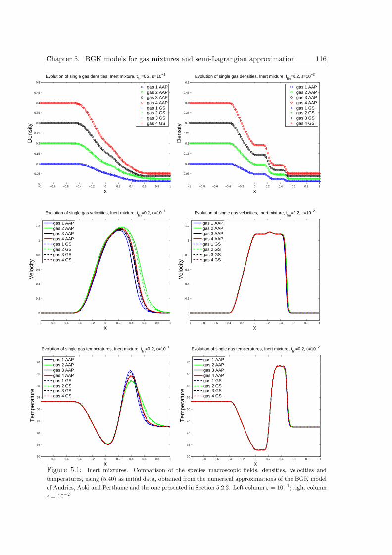
Chapter 5. BGK models for gas mixtures and semi-Lagrangian approximation 116
−1 −0.8 −0.6 −0.4 −0.2 0 0.2 0.4 0.6 0.8 10
0.05
0.1
0.15
0.2
0.25
0.3
0.35
0.4
0.45
0.5
Evolution of single gas densities, Inert mixture, tfin
=0.2, ε=10−1
x
Den
sity
gas 1 AAPgas 2 AAPgas 3 AAPgas 4 AAPgas 1 GSgas 2 GSgas 3 GSgas 4 GS
−1 −0.8 −0.6 −0.4 −0.2 0 0.2 0.4 0.6 0.8 10
0.05
0.1
0.15
0.2
0.25
0.3
0.35
0.4
0.45
0.5
Evolution of single gas densities, Inert mixture, tfin
=0.2, ε=10−2
x
Den
sity
gas 1 AAPgas 2 AAPgas 3 AAPgas 4 AAPgas 1 GSgas 2 GSgas 3 GSgas 4 GS
−1 −0.8 −0.6 −0.4 −0.2 0 0.2 0.4 0.6 0.8 1
0
0.2
0.4
0.6
0.8
1
1.2
Evolution of single gas velocities, Inert mixture, tfin
=0.2, ε=10−1
x
Vel
ocity
gas 1 AAPgas 2 AAPgas 3 AAPgas 4 AAPgas 1 GSgas 2 GSgas 3 GSgas 4 GS
−1 −0.8 −0.6 −0.4 −0.2 0 0.2 0.4 0.6 0.8 1
0
0.2
0.4
0.6
0.8
1
1.2
Evolution of single gas velocities, Inert mixture, tfin
=0.2, ε=10−2
x
Vel
ocity
gas 1 AAPgas 2 AAPgas 3 AAPgas 4 AAPgas 1 GSgas 2 GSgas 3 GSgas 4 GS
−1 −0.8 −0.6 −0.4 −0.2 0 0.2 0.4 0.6 0.8 130
35
40
45
50
55
60
65
70
Evolution of single gas temperatures, Inert mixture, tfin
=0.2, ε=10−1
x
Tem
pera
ture
gas 1 AAPgas 2 AAPgas 3 AAPgas 4 AAPgas 1 GSgas 2 GSgas 3 GSgas 4 GS
−1 −0.8 −0.6 −0.4 −0.2 0 0.2 0.4 0.6 0.8 130
35
40
45
50
55
60
65
70
Evolution of single gas temperatures, Inert mixture, tfin
=0.2, ε=10−2
x
Tem
pera
ture
gas 1 AAPgas 2 AAPgas 3 AAPgas 4 AAPgas 1 GSgas 2 GSgas 3 GSgas 4 GS
Figure 5.1: Inert mixtures. Comparison of the species macroscopic fields, densities, velocities and
temperatures, using (5.40) as initial data, obtained from the numerical approximations of the BGK model
of Andries, Aoki and Perthame and the one presented in Section 5.2.2. Left column ε = 10−1; right column
ε = 10−2.
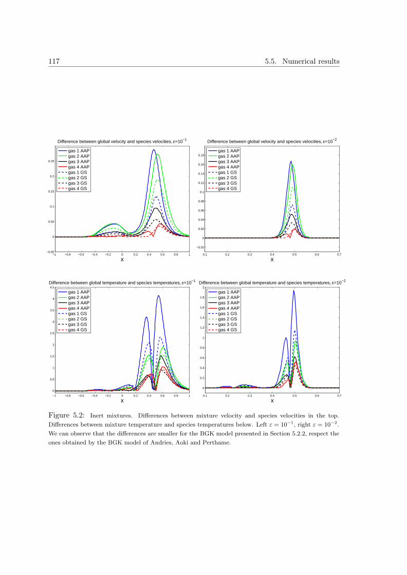
117 5.5. Numerical results
−1 −0.8 −0.6 −0.4 −0.2 0 0.2 0.4 0.6 0.8 1−0.05
0
0.05
0.1
0.15
0.2
0.25
Difference between global velocity and species velocities, ε=10−1
x
gas 1 AAPgas 2 AAPgas 3 AAPgas 4 AAPgas 1 GSgas 2 GSgas 3 GSgas 4 GS
0.1 0.2 0.3 0.4 0.5 0.6 0.7
−0.02
0
0.02
0.04
0.06
0.08
0.1
0.12
0.14
0.16
0.18
Difference between global velocity and species velocities, ε=10−2
x
gas 1 AAPgas 2 AAPgas 3 AAPgas 4 AAPgas 1 GSgas 2 GSgas 3 GSgas 4 GS
−1 −0.8 −0.6 −0.4 −0.2 0 0.2 0.4 0.6 0.8 1
0
0.5
1
1.5
2
2.5
3
3.5
4
4.5Difference between global temperature and species temperatures, ε=10−1
x
gas 1 AAPgas 2 AAPgas 3 AAPgas 4 AAPgas 1 GSgas 2 GSgas 3 GSgas 4 GS
0.1 0.2 0.3 0.4 0.5 0.6 0.7
0
0.2
0.4
0.6
0.8
1
1.2
1.4
1.6
1.8
2Difference between global temperature and species temperatures, ε=10−2
x
gas 1 AAPgas 2 AAPgas 3 AAPgas 4 AAPgas 1 GSgas 2 GSgas 3 GSgas 4 GS
Figure 5.2: Inert mixtures. Differences between mixture velocity and species velocities in the top.
Differences between mixture temperature and species temperatures below. Left ε = 10−1, right ε = 10−2.
We can observe that the differences are smaller for the BGK model presented in Section 5.2.2, respect the
ones obtained by the BGK model of Andries, Aoki and Perthame.
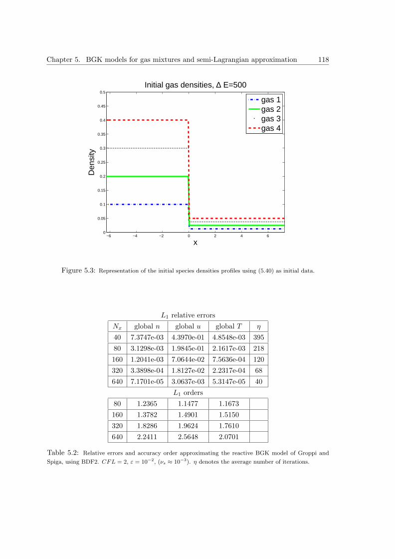
Chapter 5. BGK models for gas mixtures and semi-Lagrangian approximation 118
−6 −4 −2 0 2 4 60
0.05
0.1
0.15
0.2
0.25
0.3
0.35
0.4
0.45
0.5
Initial gas densities, ∆ E=500
x
Den
sity
gas 1gas 2gas 3gas 4
Figure 5.3: Representation of the initial species densities profiles using (5.40) as initial data.
L1 relative errors
Nx global n global u global T η
40 7.3747e-03 4.3970e-01 4.8548e-03 395
80 3.1298e-03 1.9845e-01 2.1617e-03 218
160 1.2041e-03 7.0644e-02 7.5636e-04 120
320 3.3898e-04 1.8127e-02 2.2317e-04 68
640 7.1701e-05 3.0637e-03 5.3147e-05 40
L1 orders
80 1.2365 1.1477 1.1673
160 1.3782 1.4901 1.5150
320 1.8286 1.9624 1.7610
640 2.2411 2.5648 2.0701
Table 5.2: Relative errors and accuracy order approximating the reactive BGK model of Groppi and
Spiga, using BDF2. CFL = 2, ε = 10−2, (νs ≈ 10−3). η denotes the average number of iterations.
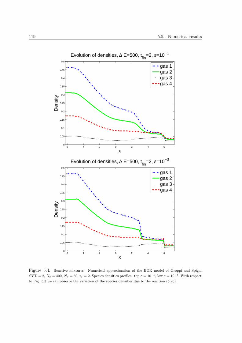
119 5.5. Numerical results
−6 −4 −2 0 2 4 60
0.05
0.1
0.15
0.2
0.25
0.3
0.35
0.4
0.45
0.5
Evolution of densities, ∆ E=500, tfin
=2, ε=10−1
x
Den
sity
gas 1gas 2gas 3gas 4
−6 −4 −2 0 2 4 60
0.05
0.1
0.15
0.2
0.25
0.3
0.35
0.4
0.45
0.5
Evolution of densities, ∆ E=500, tfin
=2, ε=10−3
x
Den
sity
gas 1gas 2gas 3gas 4
Figure 5.4: Reactive mixtures. Numerical approximation of the BGK model of Groppi and Spiga.
CFL = 2, Nx = 400, Nv = 60, tf = 2. Species densities profiles: top ε = 10−1, low ε = 10−3. With respect
to Fig. 5.3 we can observe the variation of the species densities due to the reaction (5.20).
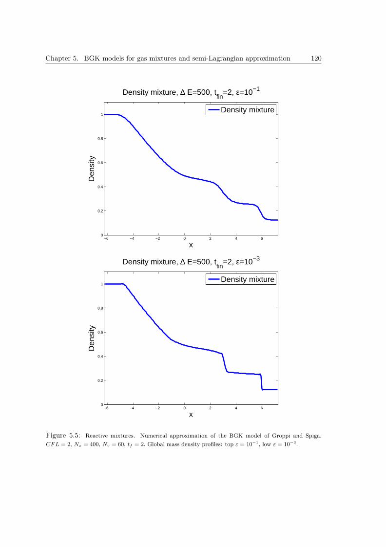
Chapter 5. BGK models for gas mixtures and semi-Lagrangian approximation 120
−6 −4 −2 0 2 4 60
0.2
0.4
0.6
0.8
1
Density mixture, ∆ E=500, tfin
=2, ε=10−1
x
Den
sity
Density mixture
−6 −4 −2 0 2 4 60
0.2
0.4
0.6
0.8
1
Density mixture, ∆ E=500, tfin
=2, ε=10−3
x
Den
sity
Density mixture
Figure 5.5: Reactive mixtures. Numerical approximation of the BGK model of Groppi and Spiga.
CFL = 2, Nx = 400, Nv = 60, tf = 2. Global mass density profiles: top ε = 10−1, low ε = 10−3.
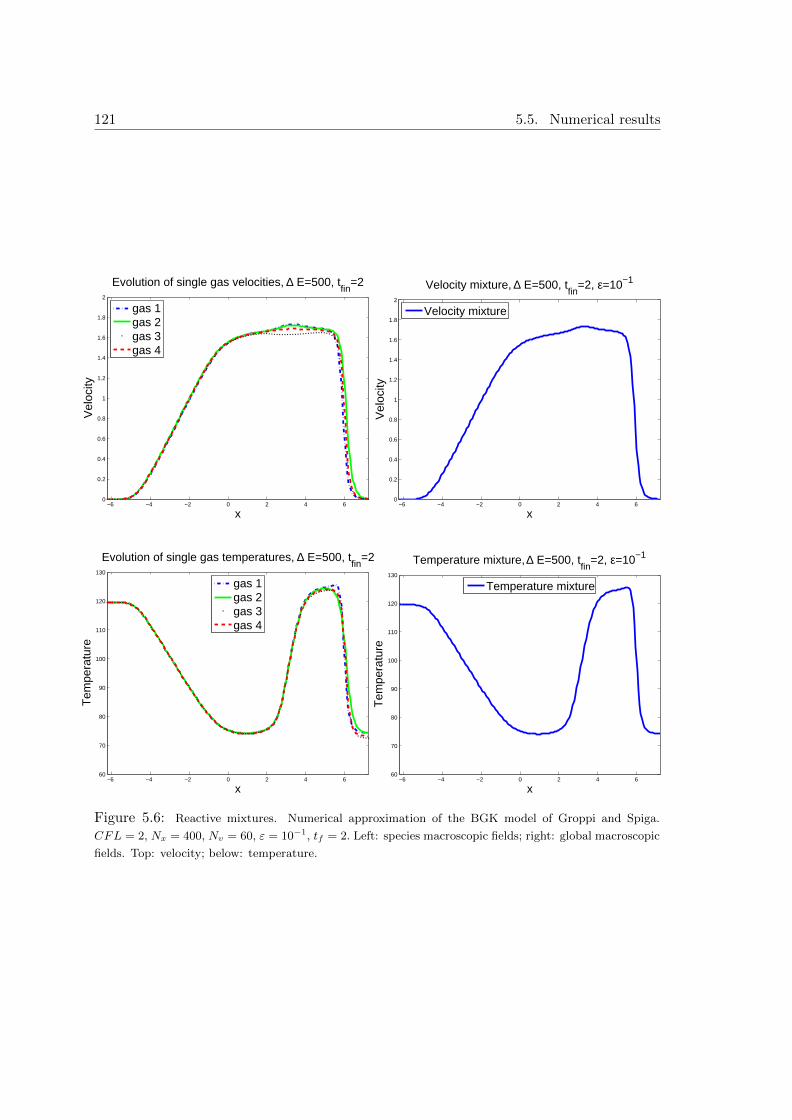
121 5.5. Numerical results
−6 −4 −2 0 2 4 60
0.2
0.4
0.6
0.8
1
1.2
1.4
1.6
1.8
2
Evolution of single gas velocities, ∆ E=500, tfin
=2
x
Vel
ocity
gas 1gas 2gas 3gas 4
−6 −4 −2 0 2 4 60
0.2
0.4
0.6
0.8
1
1.2
1.4
1.6
1.8
2
Velocity mixture, ∆ E=500, tfin
=2, ε=10−1
x
Vel
ocity
Velocity mixture
−6 −4 −2 0 2 4 660
70
80
90
100
110
120
130
Evolution of single gas temperatures, ∆ E=500, tfin
=2
x
Tem
pera
ture
gas 1gas 2gas 3gas 4
−6 −4 −2 0 2 4 660
70
80
90
100
110
120
130
Temperature mixture, ∆ E=500, tfin
=2, ε=10−1
x
Tem
pera
ture
Temperature mixture
Figure 5.6: Reactive mixtures. Numerical approximation of the BGK model of Groppi and Spiga.
CFL = 2, Nx = 400, Nv = 60, ε = 10−1, tf = 2. Left: species macroscopic fields; right: global macroscopic
fields. Top: velocity; below: temperature.
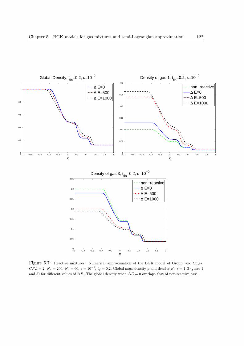
Chapter 5. BGK models for gas mixtures and semi-Lagrangian approximation 122
−1 −0.8 −0.6 −0.4 −0.2 0 0.2 0.4 0.6 0.8 10
0.2
0.4
0.6
0.8
1
Global Density, tfin
=0.2, ε=10−2
x
∆ E=0∆ E=500∆ E=1000
−1 −0.8 −0.6 −0.4 −0.2 0 0.2 0.4 0.6 0.8 10
0.05
0.1
0.15
0.2
0.25
0.3
Density of gas 1, tfin
=0.2, ε=10−2
x
non−reactive∆ E=0∆ E=500∆ E=1000
−1 −0.8 −0.6 −0.4 −0.2 0 0.2 0.4 0.6 0.8 10
0.05
0.1
0.15
0.2
0.25
0.3
0.35
Density of gas 3, tfin
=0.2, ε=10−2
x
non−reactive∆ E=0∆ E=500∆ E=1000
Figure 5.7: Reactive mixtures. Numerical approximation of the BGK model of Groppi and Spiga.
CFL = 2, Nx = 200, Nv = 60, ε = 10−2, tf = 0.2. Global mass density ρ and density ρs, s = 1, 3 (gases 1
and 3) for different values of ∆E. The global density when ∆E = 0 overlaps that of non-reactive case.
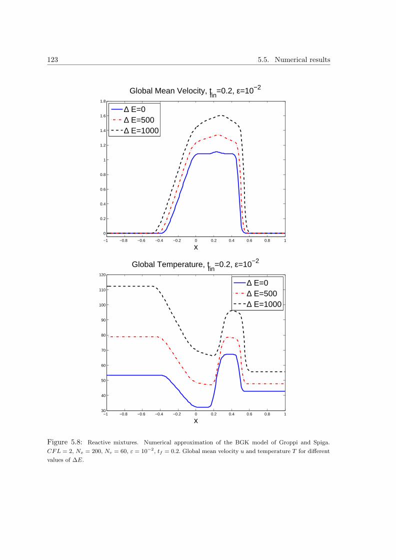
123 5.5. Numerical results
−1 −0.8 −0.6 −0.4 −0.2 0 0.2 0.4 0.6 0.8 1
0
0.2
0.4
0.6
0.8
1
1.2
1.4
1.6
1.8
Global Mean Velocity, tfin
=0.2, ε=10−2
x
∆ E=0∆ E=500∆ E=1000
−1 −0.8 −0.6 −0.4 −0.2 0 0.2 0.4 0.6 0.8 130
40
50
60
70
80
90
100
110
120
Global Temperature, tfin
=0.2, ε=10−2
x
∆ E=0∆ E=500∆ E=1000
Figure 5.8: Reactive mixtures. Numerical approximation of the BGK model of Groppi and Spiga.
CFL = 2, Nx = 200, Nv = 60, ε = 10−2, tf = 0.2. Global mean velocity u and temperature T for different
values of ∆E.

Chapter 5. BGK models for gas mixtures and semi-Lagrangian approximation 124
Conclusions and Perspectives
This thesis focuses on high order shock capturing semi-Lagrangian methods for the nu-
merical solutions of BGK-type equations.
The methods are based on L-stable schemes for the solution of the BGK equations along
the characteristics, and are asymptotic preserving, in the sense that they are able to cap-
ture the fluid dynamic limit.
Two families of schemes are presented, which differ for the choice of the time integrator,
Runge-Kutta or BDF, respectively. A further distinction concerns space discretization:
some schemes are based on high order reconstruction, while others are constructed on the
lattice in phase space, thus requiring no space interpolation.
Numerical experiments show that schemes without interpolation can be cost-effective, es-
pecially for problems that do not require a fine mesh in velocity. In particular, BDF3
without interpolation appears to have the best performance in most tests.
We investigated some applications and extensions to more physical interesting problems
of the numerical schemes proposed for the one dimensional BGK equation. By means of
the Chu reduction [15], we extended the schemes to more realistic physical domains, 3D in
velocity. Moreover, we considered boundary-value problems and we studied the treatment
of reflective and diffusive boundary conditions. Two numerical techniques to deal with
diffusive boundary conditions are presented. The numerical results obtained are in good
agreement with the ones present in literature [19].
Finally, the methods have been extended to different BGK models for inert [3] and reactive
[25] gas mixtures in three dimensional velocity space.
Future plans includes extension of such schemes to problems in several space dimensions
and treatment of more general boundary conditions, the case of moving boundaries. More-
over, applications of these schemes to the numerical approximation of other BGK equations
for mixtures of rarefied gases are in progress. In particular, we will investigate the dis-
125
Conclusions and Perspectives 126
cretization of the BGK model [23], that is the extension to the reactive case of the inert
BGK model (5.13).
Furthermore, on the modelling side, other BGK approximation could be developed and
then numerically solved by means of the schemes investigated in this thesis, like for in-
stance multitemperature models. Typically, relaxation to thermodynamical equilibrium
in a gas mixture might occur on different scales: for instance, when masses are disparate,
a first Maxwellization step within each species is followed by a slower equilibration of ve-
locities and temperatures [22]. Indeed, when vibrational and chemical relaxations proceed
at the slower gas-dynamic time scale, a one-temperature gas flow description is not valid
any more [32]. On the other hand, a multi-temperature approach is needed in several
problems of aerothermodynamics [9] or in plasmas at high temperatures [45]. A BGK
model for mixture, characterized by attractors with auxiliary species temperatures and
only one auxiliary global velocity, thus at an intermediate stage between the two BGK for
inert mixtures considered in this thesis, could be suitable to describe such problems.
Bibliography
[1] A. Aimi, M. Diligenti, M. Groppi, C. Guardasoni, On the numerical solution of a
BGK-type model for chemical reactions, European J. Mech. B/Fluids 26, 455-472,
2007.
[2] A. Alaia, G. Puppo, A hybrid method for hydrodynamic-kinetic flow - Part II - Cou-
pling of hydrodynamic and kinetic models, J. Comp. Phys. 231 (16), 5217–5242, 2012.
[3] P. Andries, K. Aoki and B. Perthame, A consistent BGK-type model for gas mixtures,
J. Stat. Phys. 106, 993–1018, 2002.
[4] K. Aoki, Y. Sone, and T. Yamada, Numerical analysis of gas flows condensing on its
plane condensed phase on the basis of kinetic theory, Phys. Fluids A 2, 10, 1867–1878,
1990.
[5] U. M. Ascher, S. J. Ruuth, R. J. Spiteri, Implicit-Explicit Runge-Kutta methods for
time-dependent partial differential equations, Appl. Numer. Math. 25, 151–167, 1997.
[6] G. A. Bird, Molecular Gas Dynamics and the Direct Simulation of Gas Flows, Oxford
Engineering Science Series. Clarendon Press, 1994.
[7] M. Bisi, M. Groppi, G. Spiga, Kinetic Bhatnagar-Gross-Krook model for fast reactive
mixtures and its hydrodynamic limit, Phys. Rev. E 81 036327, 1–9, 2010.
[8] P.L. Bhatnagar, E.P. Gross and K. Krook, A model for collision processes in gases,
Phys. Rev. 94, 511–525, 1954.
[9] T.K. Bose, High Temperature Gas Dynamics, Springer, Berlin, 2003.
[10] C. Buet, A discrete velocity scheme for the Boltzmann operator of rarefied gas dy-
namics, Transport Theor. Stat., 25, 33–60, 1996.
[11] E. Carlini, R. Ferretti and G. Russo, A weighted essentially nonoscillatory, large
time-step scheme for Hamilton-Jacobi equations, SIAM J. Sci. Comput. 27, 1071–
1091, 2005.
[12] R. Caflisch, The fluid dynamical limit of the nonlinear Boltzmann equation, Commun.
Pure Appl. Math., 666, 33–651,1980.
127
Bibliography 128
[13] C. Cercignani, The Boltzmann Equation and its Applications, Springer, New York,
1988.
[14] C. Cercignani, Slow Rarefied Flows: Theory and Application to Micro-Electro-
Mechanical Systems, Birkhauser, Base, 2006.
[15] C.K. Chu, Kinetic-theoretic description of the formation of a shock wave, Phys. Fluids
8, 12–21, 1965.
[16] G. Dimarco, R. Loubere, Towards an ultra efficient kinetic scheme. Part I: Basics on
the BGK equation, J. Comput. Phys. 255, 680–698, 2013.
[17] G. Dimarco, R. Loubere, Towards an ultra efficient kinetic scheme. Part II: The high
order case, J. Comput. Phys. 255, 699–719, 2013.
[18] M. Falcone , R. Ferretti, Semi-Lagrangian Approximation Schemes For Linear And
Hamilton-Jacobi Equations, SIAM, Philadelphia, 2014.
[19] F. Filbet, C. Yang, Inverse Lax-Wendroff method for boundary conditions of Boltz-
mann type models, arXiv:1209.3103 [math.NA], 12 September 2012.
[20] F. Filbet, G. Russo, Semilagrangian schemes applied to moving boundary problems
for the BGK model of rarefied gas dynamics, Kinet. Relat. Models 2, 231–250, 2009.
[21] V.Garzo, A. Santos, J. J. Brey, A kinetic model for a multicomponent gas, Phys.
Fluids A, 1(2), 380–383, 1989.
[22] E. Goldman, L.Sirovich, Equations for gas mixtures, Phys. Fluids, 10(9), 1928–1940,
1967.
[23] M. Groppi, S. Rjasanow, G. Spiga, A kinetic relaxation approach to fast reactive
mixtures: shock wave structure, J. Stat. Mech., 1–15, 2009.
[24] M. Groppi, G. Russo, G. Stracquadanio., High order semi-Lagrangian methods for
BGK models. Preprint n.519, Department of Mathematics and Computer Science,
University of Parma, 2014, submitted.
[25] M. Groppi, G. Spiga, A Bhatnagar-Gross-Krook type approach for chemically reacting
gas mixtures, Phys. Fluids 16, 4273–4284, 2004.
[26] E. P. Gross, M. Krook, Model for collision processes in gases: Small-amplitude oscil-
lations of charged two-component systems, Phys. Rev, 102, 593, 1956.
[27] E. Hairer, S.P. Nørsett, G. Warner, Solving Ordinary Differential Equations I: Non-
Stiff Problems, Springer Series in Computational Mathematics 8. Springer, Berlin,
1987.
129 Bibliography
[28] E. Hairer, G. Warner, Solving Ordinary Differential Equations II: Stiff and
Differential-Algebraic Problems, Springer Series in Computational Mathematics 14.
Springer, Berlin, 1991.
[29] L.H. Holway, New statistical models for kinetic theory: methods of construction, Phys.
Fluids 9, 1658–1673, 1966.
[30] L. Huang, C.-W. Shu and M. Zhang, Numerical boundary conditions for the fast
sweeping high order WENO methods for solving the Eikonal equation, J. Comput.
Math., 26, 336–46, 2008.
[31] S. Jin, Efficient asymptotic-preserving (AP) schemes for some multiscale kinetic equa-
tions, SIAM J. Sci. Comput., 21, 441–452, 1999.
[32] E. Kustova, E. Nagnibeda, On a correct description of a multi-temperature dissociat-
ing CO2 flow, Chem. Phys., 321, 293–310, 2006.
[33] R.J. LeVeque, Numerical methods for conservation laws, Lectures in Mathematics,
ETH-Zurich Birkhauser-Verlag, Basel, 1990.
[34] R.J. LeVeque, Finite volume methods for hyperbolic problems, Cambridge University
Press, 2002.
[35] J. C. Maxwell, Phil. Trans. Royal Soc. I, Appendix, 1879; reprinted in The Scientific
Parers of J. C. Maxwell, Dover Publications, 1965.
[36] L. Mieussens, Discrete-velocity models and numerical schemes for the Boltzmann-
BGK equation in plane and axisymmetric geometries, J. Comp. Phys. 162 (2), 429–
466, 2000.
[37] L. Mieussens, Discrete velocity model and implicit scheme for the BGK equation of
rarefied gas dynamics, Math. Models Meth. Appl. Sci. 10, 1121–1149, 2000.
[38] T. Nishida, Fluid dynamical limit of the nonlinear Boltzmann equation at the level of
the compressible euler equations, Commun. Math. Phys., 148, 61–119, 1978.
[39] L. Pareschi, G. Russo, Efficient asymptotic preserving deterministic methods for the
Boltzmann equation, AVT-194 RTO AVT/VKI, Models and Computational Meth-
ods for Rarefied Flows, Lecture Series held at the von Karman Institute, Rhode St.
Genese, Belgium, 24 -28 January 2011.
[40] L. Pareschi and G. Russo, Implicit-explicit Runge-Kutta methods and applications to
hyperbolic systems with relaxation, J. Sci. Comp. 25, 129–155, 2005.
[41] B. Perthame, Global existence to the BGK model of Boltzmann equation, J. Differ.
Equations 82, 191–205, 1989.
Bibliography 130
[42] S. Pieraccini, G. Puppo, Implicit-explicit schemes for BGK kinetic equations, J. Sci.
Comput. 32, 1–28, 2007.
[43] S. Pieraccini, G. Puppo, Microscopically implicit-macroscopically explicit schemes for
the BGK equation, J. Comput. Phys. 231, 299–327, 2012.
[44] G. Puppo, personal communications, 2013.
[45] J.D. Ramshaw, Hydrodynamic theory of multicomponent diffusion and thermal- dif-
fusion in multitemperature gas mixtures, J. Non–Equilib. Thermodyn., 18, 121–134,
1993.
[46] F. Rogier, J. Schneider, A direct method for solving the Boltzmann Equation, Trans-
port Theor. Stat., 23, 313–338, 1994.
[47] A. Rossani, G. Spiga, A note on the kinetic theory of chemically reacting gases,
Physica A, 272, 563–573, 1999.
[48] G. Russo, High Order Shock-Capturing Schemes for Balance Laws, in: S.Bertoluzza,
S. Falletta, G. Russo, C-W. Shu, Numerical Solution of Partial Differential Equations,
Advanced Courses in Mathematics CRM Barcelona, Birkhauser, Basel, 2009.
[49] G. Russo, P. Santagati, S.-B. Yun, Convergence of a semi-lagrangian scheme for the
BGK model of the Boltzmann equation, SIAM J. Numer. Anal. 50, 1111–1135, 2012.
[50] G. Russo and P. Santagati, A new class of large time step methods for the BGK
models of the Boltzmann equation, arXiv:1103.5247v1, 2011.
[51] P. Santagati, High order semi-Lagrangian schemes for the BGK model of the Boltz-
mann equation, Department of Mathematics and Computer Science, University of
Catania, PhD. thesis, 2007.
[52] L. Sivorich, Kinetic modeling of gas mixtures, Phys. Fluids, 5, 908–918, 1962.
[53] C.W. Shu, Essentially non-oscillatory and weighted essentially non-oscillatory
schemes for hyperbolic conservation laws, in Advanced Numerical Approximation
of Nonlinear Hyperbolic Equations, Lecture Notes in Math. 1697, Papers from the
C.I.M.E. Summer School held in Certraro, June 23-28, 1997, A. Quarteroni, Ed.
Springer-Verlag, Berlin, 1998.
[54] S. Tan, C.W. Shu, Inverse Lax-Wendroff procedure for numerical boundary conditions
of conservation laws, J. Comput. Phys., 229, 8144–8166, 2010.
[55] S. Tan and C.W. Shu, A high order moving boundary treatment for compressible
inviscid flows, J. Comput. Phys., 230, 6023–6036, 2011.
[56] S. Tan, C. Wang, C.W. Shu, J. Ning, Efficient implementation of high order inverse
Lax-Wendroff boundary treatment for conservation laws, J. Comput. Phys., 231, 2510–
2527, 2012.
131 Bibliography
[57] L. Saint-Raymond, From the BGK model to the Navier-Stokes equations, Ann. Scient.
Ec. Norm. Sup. 36, 271–317, 2003.
[58] P. Welander, On the temperature jump in a rarefied gas, Ark. Fys. 7, 507–553, 1954.
[59] T. Xiong, M. Zhang, Y.-T. Zhang and C.-W. Shu, Fast sweeping fifth order WENO
scheme for static Hamilton-Jacobi equations with accurate boundary treatment, J. Sci.
Comput., 45, 514–536, 2010.
[60] S. Yun, Cauchy problem for the Boltzmann-BGK model near a global Maxwellian, J.
Math. Phys. 51, 123514, 2010.
Recommended