Uniovi 1
Some distributions
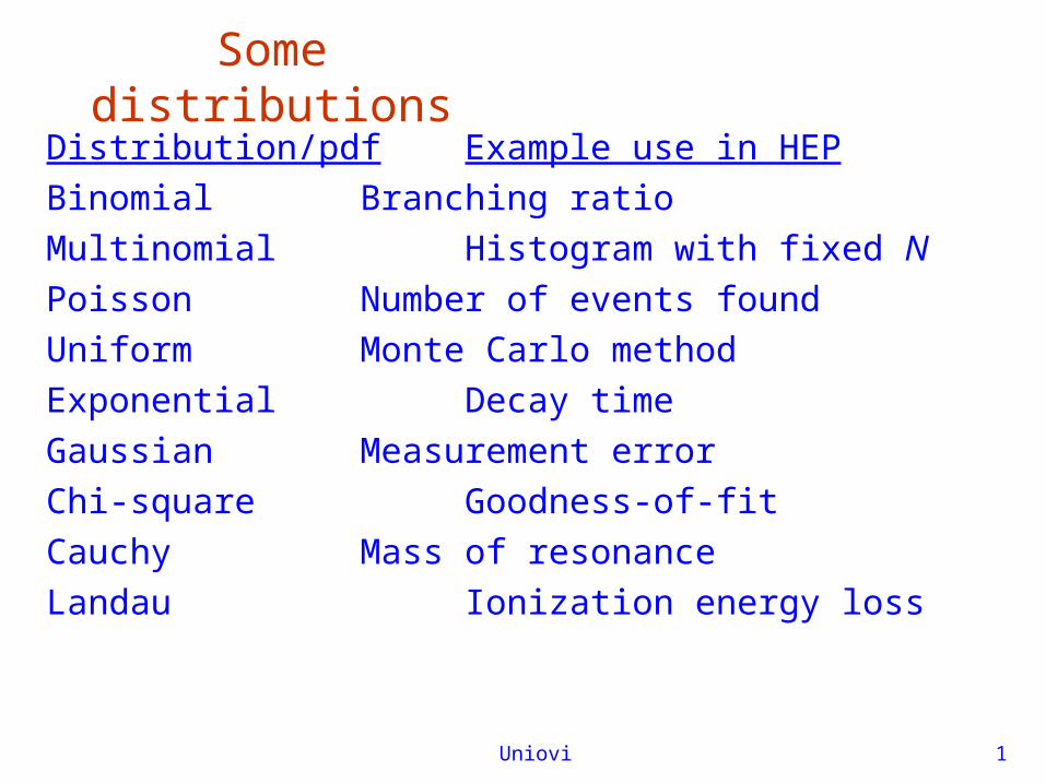
Distribution/pdf Example use in HEP
Binomial Branching ratio
Multinomial Histogram with fixed N
Poisson Number of events found
Uniform Monte Carlo method
Exponential Decay time
Gaussian Measurement error
Chi-square Goodness-of-fit
Cauchy Mass of resonance
Landau Ionization energy loss
Uniovi 2
Binomial distribution
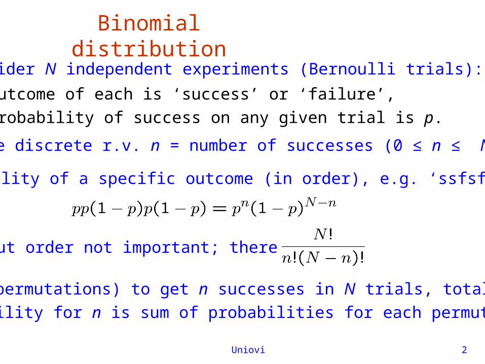
Consider N independent experiments (Bernoulli trials):
outcome of each is ‘success’ or ‘failure’,
probability of success on any given trial is p.
Define discrete r.v. n = number of successes (0 ≤ n ≤ N).
Probability of a specific outcome (in order), e.g. ‘ssfsf’ is
But order not important; there are
ways (permutations) to get n successes in N trials, total
probability for n is sum of probabilities for each permutation.
Uniovi 3
Binomial distribution (2)
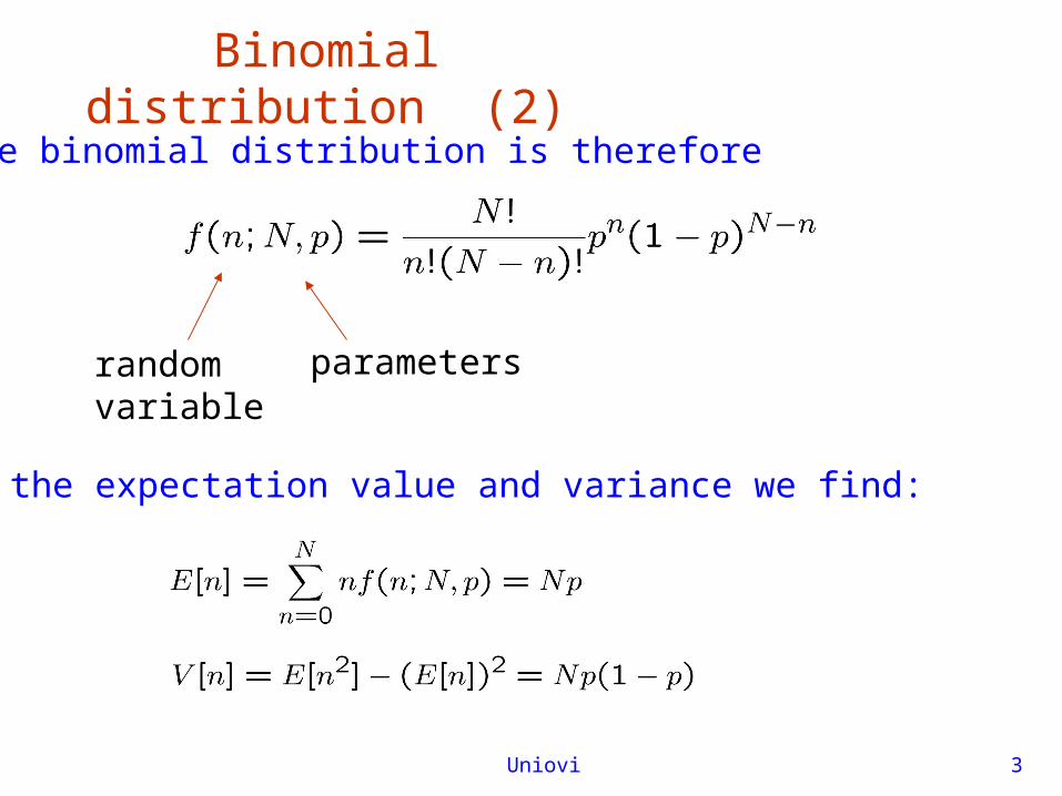
The binomial distribution is therefore
randomvariable
parameters
For the expectation value and variance we find:
Uniovi 4
Binomial distribution (3)
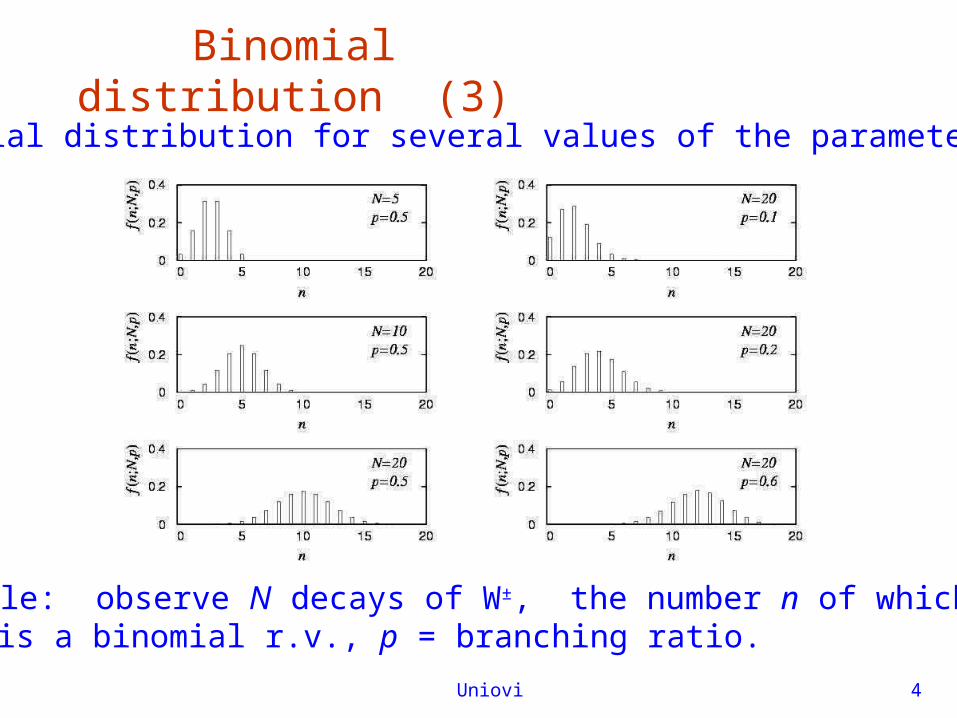
Binomial distribution for several values of the parameters:
Example: observe N decays of W±, the number n of which are W→ is a binomial r.v., p = branching ratio.
Uniovi 5
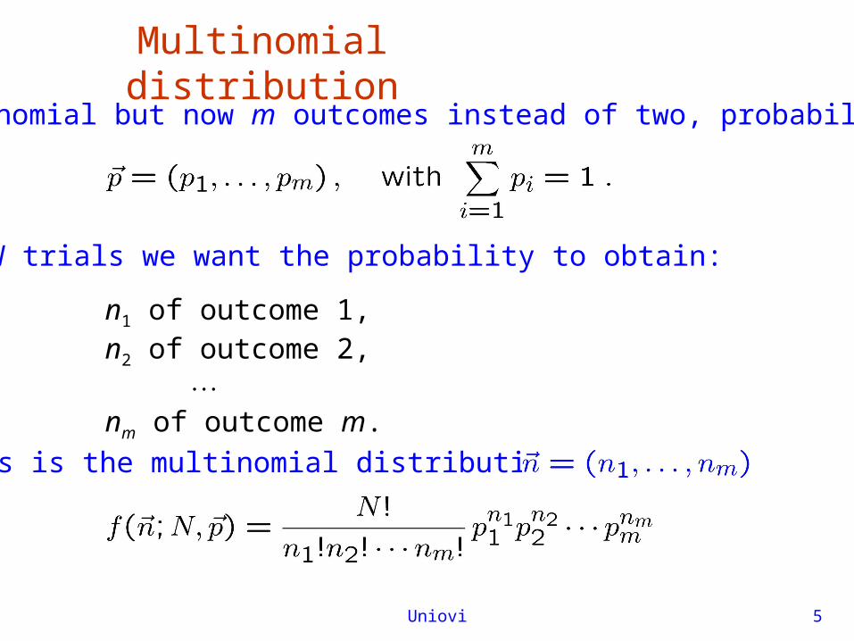
Multinomial distributionLike binomial but now m outcomes instead of two, probabilities are
For N trials we want the probability to obtain:
n1 of outcome 1,n2 of outcome 2,
nm of outcome m.
This is the multinomial distribution for
Uniovi 6
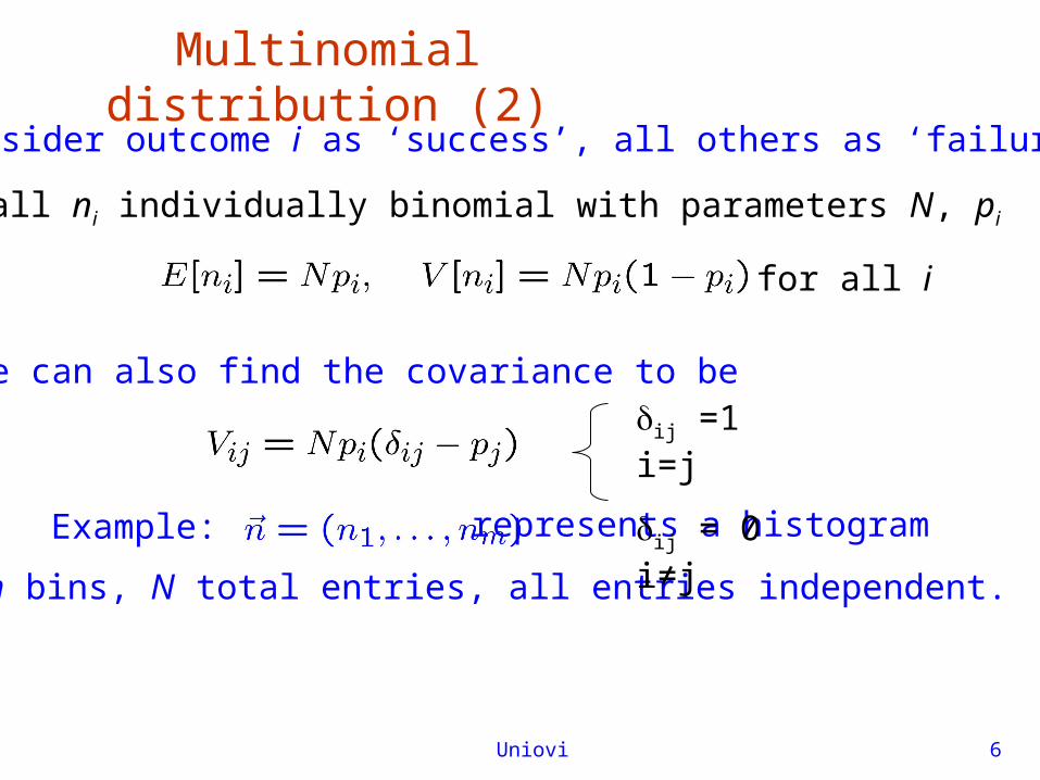
Multinomial distribution (2)Now consider outcome i as ‘success’, all others as ‘failure’.
→ all ni individually binomial with parameters N, pi
for all i
One can also find the covariance to be
Example: represents a histogram
with m bins, N total entries, all entries independent.
ij =1 i=j
ij = 0 i≠j
Uniovi 7
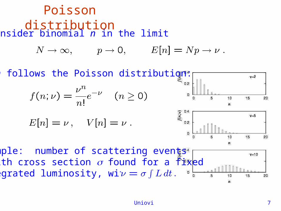
Poisson distributionConsider binomial n in the limit
→ n follows the Poisson distribution:
Example: number of scattering eventsn with cross section found for a fixedintegrated luminosity, with
Uniovi 8
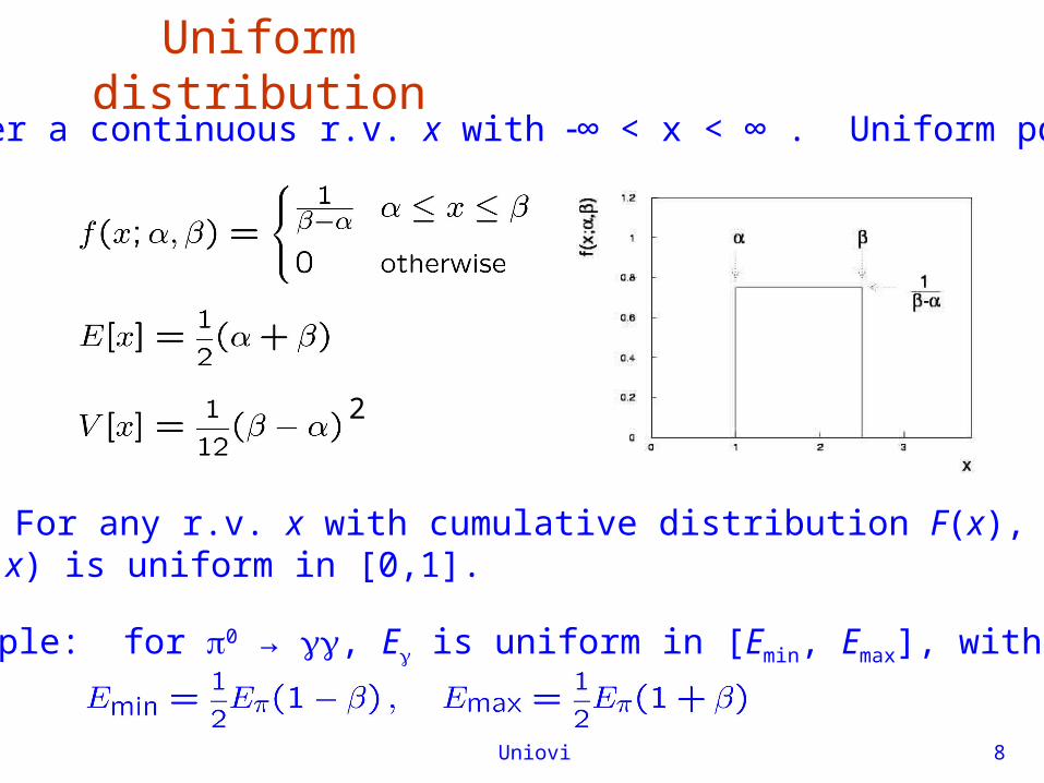
Uniform distributionConsider a continuous r.v. x with ∞ < x < ∞ . Uniform pdf is:
N.B. For any r.v. x with cumulative distribution F(x),y = F(x) is uniform in [0,1].
Example: for 0 → , E is uniform in [Emin, Emax], with
2
Uniovi 9
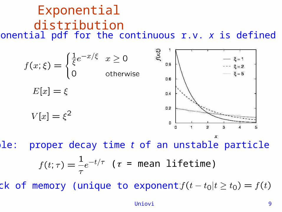
Exponential distributionThe exponential pdf for the continuous r.v. x is defined by:
Example: proper decay time t of an unstable particle
( = mean lifetime)
Lack of memory (unique to exponential):
Uniovi 10
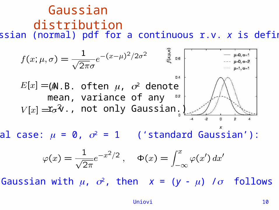
Gaussian distributionThe Gaussian (normal) pdf for a continuous r.v. x is defined by:
Special case: = 0, 2 = 1 (‘standard Gaussian’):
(N.B. often , 2 denotemean, variance of anyr.v., not only Gaussian.)
If y ~ Gaussian with , 2, then x = (y ) / follows (x).
Uniovi 11
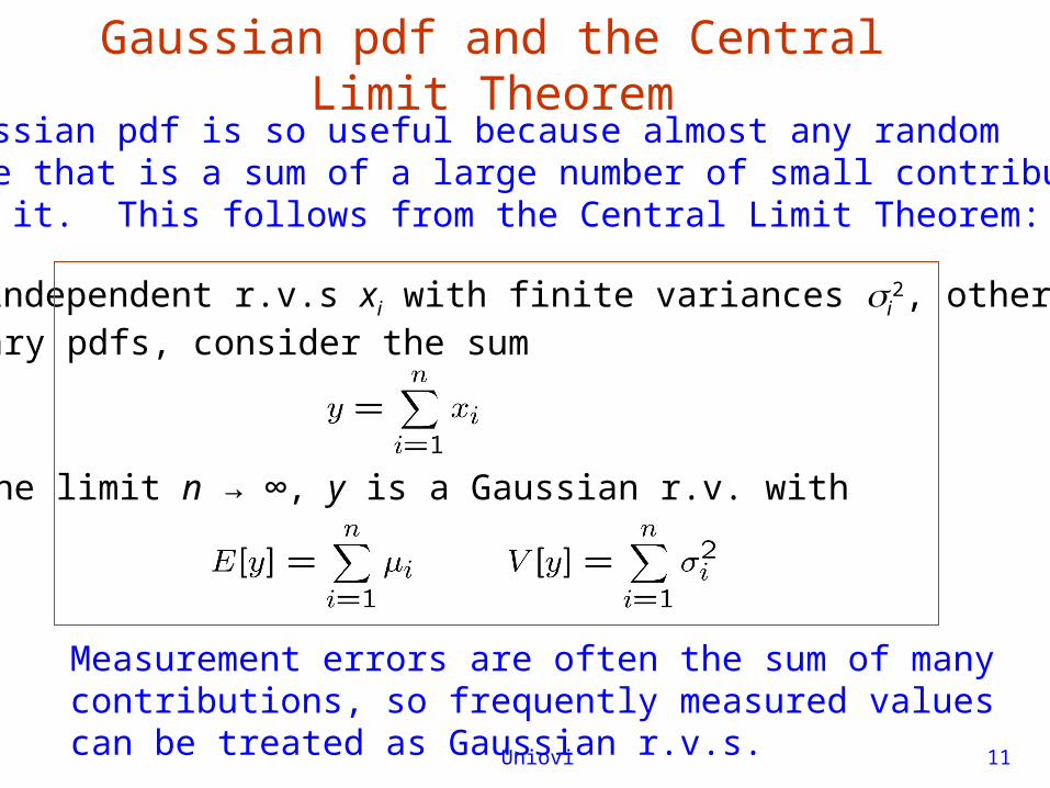
Gaussian pdf and the Central Limit TheoremThe Gaussian pdf is so useful because almost any randomvariable that is a sum of a large number of small contributionsfollows it. This follows from the Central Limit Theorem:
For n independent r.v.s xi with finite variances i2, otherwise
arbitrary pdfs, consider the sum
Measurement errors are often the sum of many contributions, so frequently measured values can be treated as Gaussian r.v.s.
In the limit n → ∞, y is a Gaussian r.v. with
Uniovi 12
Central Limit Theorem (2)The CLT can be proved using characteristic functions (Fouriertransforms), see, e.g., SDA Chapter 10.
Good example: velocity component vx of air molecules.
OK example: total deflection due to multiple Coulomb scattering.(Rare large angle deflections give non-Gaussian tail.)
Bad example: energy loss of charged particle traversing thingas layer. (Rare collisions make up large fraction of energy loss,cf. Landau pdf.)
For finite n, the theorem is approximately valid to theextent that the fluctuation of the sum is not dominated byone (or few) terms.
Beware of measurement errors with non-Gaussian tails.
Uniovi 13
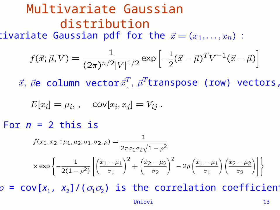
Multivariate Gaussian distribution
Multivariate Gaussian pdf for the vector
are column vectors, are transpose (row) vectors,
For n = 2 this is
where = cov[x1, x2]/(12) is the correlation coefficient.
Uniovi 14
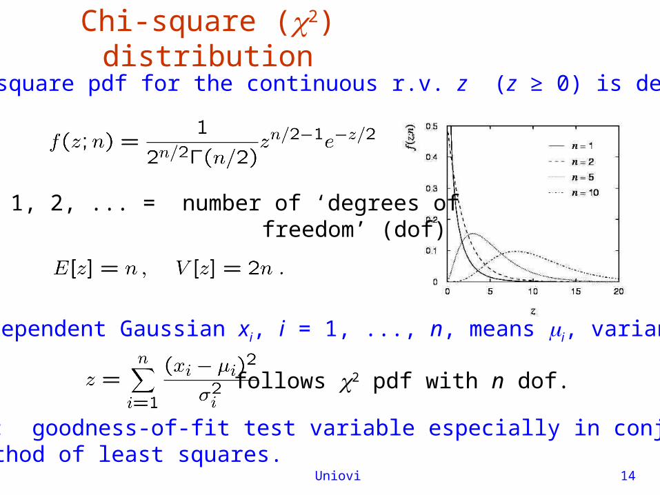
Chi-square (2) distribution
The chi-square pdf for the continuous r.v. z (z ≥ 0) is defined by
n = 1, 2, ... = number of ‘degrees of freedom’ (dof)
For independent Gaussian xi, i = 1, ..., n, means i, variances i2,
follows 2 pdf with n dof.
Example: goodness-of-fit test variable especially in conjunctionwith method of least squares.
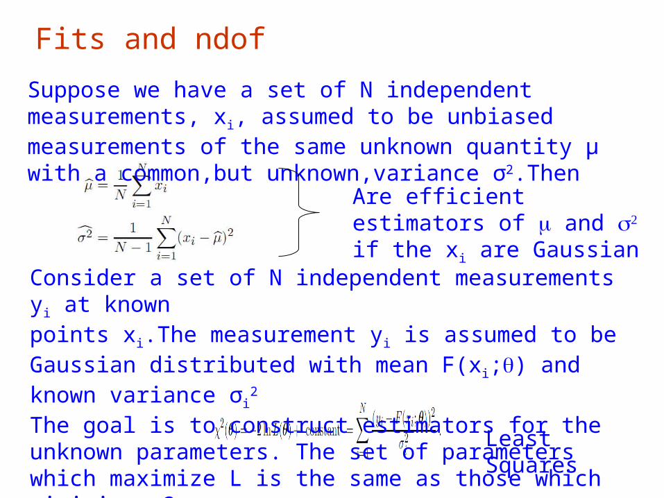
Fits and ndof
Suppose we have a set of N independent measurements, xi, assumed to be unbiased measurements of the same unknown quantity μ with a common,but unknown,variance σ2.Then
Are efficient estimators of and if the xi are Gaussian
Consider a set of N independent measurements yi at knownpoints xi.The measurement yi is assumed to be Gaussian distributed with mean F(xi;) and known variance σi
2
The goal is to construct estimators for the unknown parameters. The set of parameters which maximize L is the same as those which minimize χ2:
Least Squares
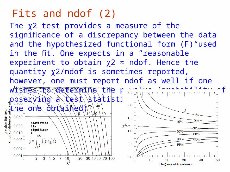
Fits and ndof (2)The χ2 test provides a measure of the significance of a discrepancy between the data and the hypothesized functional form (F) used in the fit. One expects in a “reasonable” experiment to obtain χ2 ≈ ndof. Hence the quantity χ2/ndof is sometimes reported, however, one must report ndof as well if one wishes to determine the p-value (probability of observing a test statistic at least as extreme as the one obtained)
p
n
Statistically significant
Uniovi 17
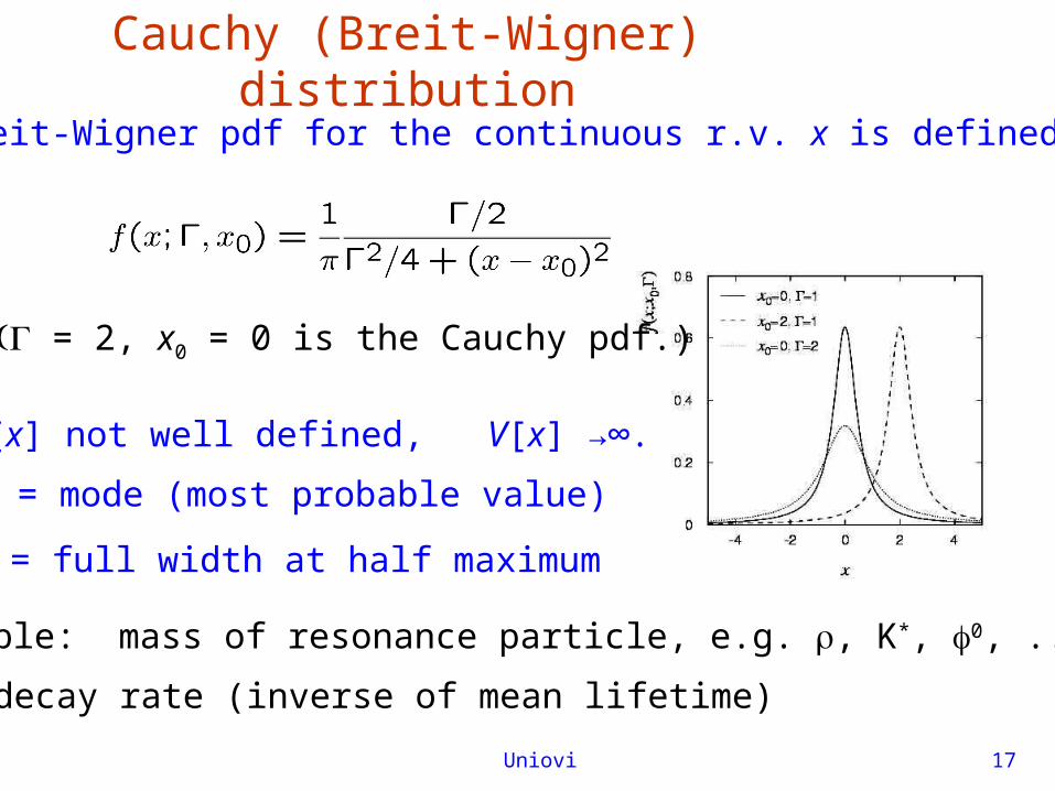
Cauchy (Breit-Wigner) distribution
The Breit-Wigner pdf for the continuous r.v. x is defined by
= 2, x0 = 0 is the Cauchy pdf.)
E[x] not well defined, V[x] →∞.
x0 = mode (most probable value)
= full width at half maximum
Example: mass of resonance particle, e.g. , K*, 0, ...
= decay rate (inverse of mean lifetime)
Uniovi 18
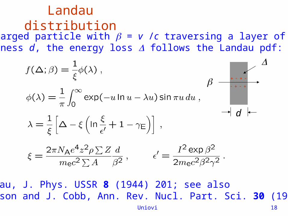
Landau distribution
For a charged particle with = v /c traversing a layer of matterof thickness d, the energy loss follows the Landau pdf:
L. Landau, J. Phys. USSR 8 (1944) 201; see alsoW. Allison and J. Cobb, Ann. Rev. Nucl. Part. Sci. 30 (1980) 253.
d
Uniovi 19
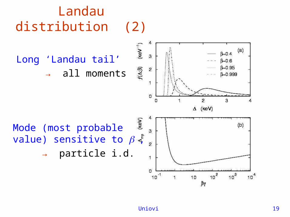
Landau distribution (2)
Long ‘Landau tail’
→ all moments
Mode (most probable value) sensitive to ,
→ particle i.d.
Uniovi 20
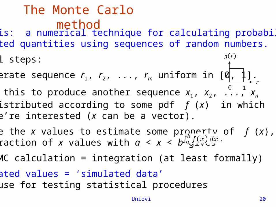
What it is: a numerical technique for calculating probabilitiesand related quantities using sequences of random numbers.
The usual steps:
(1) Generate sequence r1, r2, ..., rm uniform in [0, 1].
(2) Use this to produce another sequence x1, x2, ..., xn
distributed according to some pdf f (x) in which we’re interested (x can be a vector).
(3) Use the x values to estimate some property of f (x), e.g., fraction of x values with a < x < b gives
→ MC calculation = integration (at least formally)
MC generated values = ‘simulated data’→ use for testing statistical procedures
The Monte Carlo method
Uniovi 21
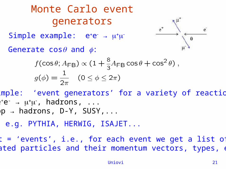
Monte Carlo event generators
Simple example: ee →
Generate cos and :
Less simple: ‘event generators’ for a variety of reactions: e+e- → , hadrons, ... pp → hadrons, D-Y, SUSY,...
e.g. PYTHIA, HERWIG, ISAJET...
Output = ‘events’, i.e., for each event we get a list ofgenerated particles and their momentum vectors, types, etc.
Uniovi 22
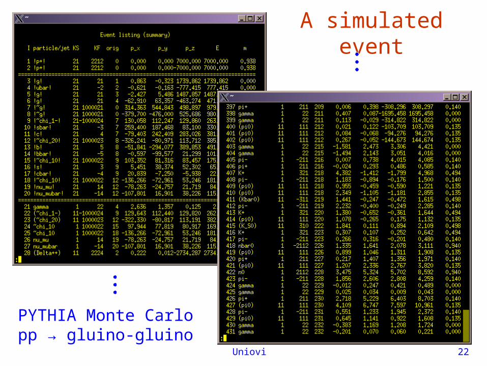
A simulated event
PYTHIA Monte Carlopp → gluino-gluino
Uniovi 23
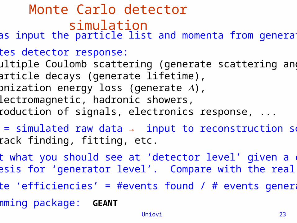
Monte Carlo detector simulationTakes as input the particle list and momenta from generator.
Simulates detector response:multiple Coulomb scattering (generate scattering angle),particle decays (generate lifetime),ionization energy loss (generate ),electromagnetic, hadronic showers,production of signals, electronics response, ...
Output = simulated raw data → input to reconstruction software:track finding, fitting, etc.
Predict what you should see at ‘detector level’ given a certain hypothesis for ‘generator level’. Compare with the real data.
Estimate ‘efficiencies’ = #events found / # events generated.
Programming package: GEANT
Uniovi 24
Random number generatorsGoal: generate uniformly distributed values in [0, 1].
Toss coin for e.g. 32 bit number... (too tiring).
→ ‘random number generator’
= computer algorithm to generate r1, r2, ..., rn.
Example: multiplicative linear congruential generator (MLCG)
ni+1 = (a ni) mod m , where
ni = integer
a = multiplier
m = modulus
n0 = seed (initial value)
N.B. mod = modulus (remainder), e.g. 27 mod 5 = 2.
This rule produces a sequence of numbers n0, n1, ...
Uniovi 25
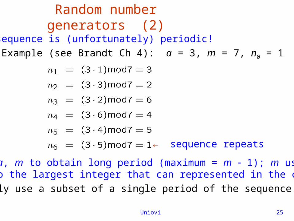
Random number generators (2)
The sequence is (unfortunately) periodic!
Example (see Brandt Ch 4): a = 3, m = 7, n0 = 1
← sequence repeats
Choose a, m to obtain long period (maximum = m 1); m usually close to the largest integer that can represented in the computer.
Only use a subset of a single period of the sequence.
Uniovi 26
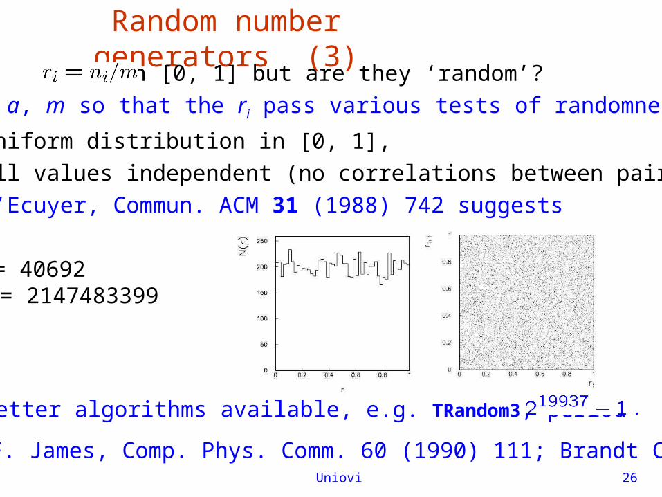
Random number generators (3)are in [0, 1] but are they ‘random’?
Choose a, m so that the ri pass various tests of randomness:
uniform distribution in [0, 1],
all values independent (no correlations between pairs),
e.g. L’Ecuyer, Commun. ACM 31 (1988) 742 suggests
a = 40692 m = 2147483399
Far better algorithms available, e.g. TRandom3, period
See F. James, Comp. Phys. Comm. 60 (1990) 111; Brandt Ch. 4
Uniovi 27
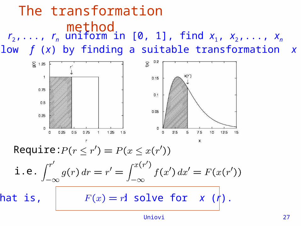
The transformation methodGiven r1, r2,..., rn uniform in [0, 1], find x1, x2,..., xn
that follow f (x) by finding a suitable transformation x (r).
Require:
i.e.
That is, set and solve for x (r).
Uniovi 28
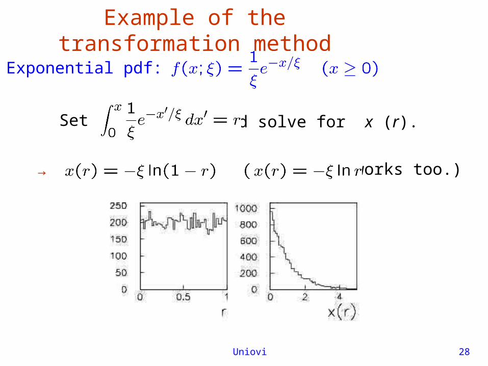
Example of the transformation method
Exponential pdf:
Set and solve for x (r).
→ works too.)
Uniovi 29
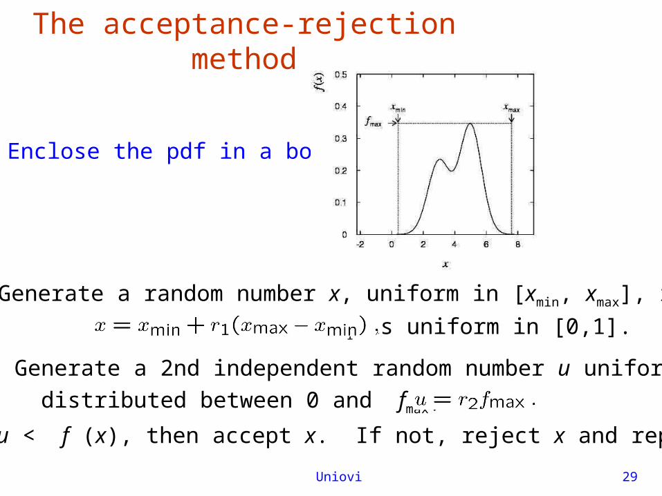
The acceptance-rejection method
Enclose the pdf in a box:
(1) Generate a random number x, uniform in [xmin, xmax], i.e.
r1 is uniform in [0,1].
(2) Generate a 2nd independent random number u uniformly
distributed between 0 and fmax, i.e.
(3) If u < f (x), then accept x. If not, reject x and repeat.
Uniovi 30
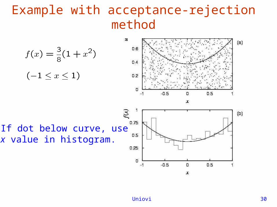
Example with acceptance-rejection method
If dot below curve, use x value in histogram.
Recommended
![NNPDF - arXiv.org e-Print archive · arXiv:1410.8849v4 [hep-ph] 4 May 2015 NNPDF Edinburgh 2014/15 IFUM-1034-FT CERN-PH-TH/2013-253 OUTP-14-11p CAVENDISH-HEP-14-11 Parton distributions](https://img.pdfslide.us/doc/110x75/5c2b5f7909d3f212718c4d3c/nnpdf-arxivorg-e-print-archive-arxiv14108849v4-hep-ph-4-may-2015-nnpdf.jpg)


![Subjet distributions in deep inelastic …0812.2864v1 [hep-ex] 15 Dec 2008 DESY–08–178 December 2008 Subjet distributions in deep inelastic scattering at HERA ZEUS Collaboration](https://img.pdfslide.us/doc/110x75/5ae0ea1a7f8b9a97518dd60e/subjet-distributions-in-deep-inelastic-08122864v1-hep-ex-15-dec-2008-desy08178.jpg)

![arXiv:1011.2692v1 [hep-ph] 11 Nov 2010 · arXiv:1011.2692v1 [hep-ph] 11 Nov 2010 Azimuthal asymmetries forhadron distributions inside ajet in hadronic collisions Umberto D’Alesio,1,2,∗](https://img.pdfslide.us/doc/110x75/5f36a3bc9c7d7a6f046220af/arxiv10112692v1-hep-ph-11-nov-2010-arxiv10112692v1-hep-ph-11-nov-2010-azimuthal.jpg)