UNIFORM POLYNOMIAL APPROXIMATION OF EVEN AND ODD FUNCTIONS ON
SYMMETRIC INTERVALS
by
CHARLES BURTON DUNHAM B.A., The U n i v e r s i t y of B r i t i s h Columbia, 1 9 5 9
A THESIS SUBMITTED IN PARTIAL FULFILMENT OF THE REQUIREMENTS FOR THE DEGREE OF
MASTER OF ARTS
In the Department
of
MATHEMATICS
We accept t h i s t h e s i s as conforming to the r e q u i r e d standard
THE UNIVERSITY OF BRITISH COLUMBIA • January, 1 9 6 3
In presenting t h i s t h e s i s i n p a r t i a l f u l f i l m e n t of
the requirements f o r an advanced degree at the U n i v e r s i t y of
B r i t i s h Columbia, I agree tha t the L i b r a r y s h a l l make i t f r e e l y
a v a i l a b l e f o r reference and study. I f u r t h e r agree that permission
f o r extensive copying of t h i s t h e s i s f o r s c h o l a r l y purposes may be
granted by the Head of my Department or by h i s representatives.
It i s understood that copying or p u b l i c a t i o n of t h i s t h e s i s f o r
f i n a n c i a l gain s h a l l not be alloxred without my written permission.
Department of ^\ ajfcAyao^J^w*-*
The U n i v e r s i t y of B r i t i s h Columbia, Vancouver S, Canada.
Date fcAh^/t^ 1% j H<3
ABSTRACT
An odd or even continuous f u n c t i o n on a symmetric i n t e r v a l C-a,a] can
be evaluated i n two d i f f e r e n t ways, each using only one uniform polynomial
approximation. I t i s of p r a c t i c a l importance t o know which method of
e v a l u a t i o n takes fewer a r i t h m e t i c operations. This i s a s p e c i a l case of a
more general problem, which i s concerned w i t h the opt i m a l s u b d i v i s i o n o f
the i n t e r v a l of e v a l u a t i o n of a f u n c t i o n f i n t o s u b - i n t e r v a l s , on each o f
which f has a uniform polynomial approximation.
In the f i r s t three chapters a method o f computing the number of
a r i t h m e t i c operations f o r e v a l u a t i o n i s developed. Expansions i n Chebyshev
polynomials are s t u d i e d , w i t h emphasis on the p r a c t i c a l problem o f computing
c o e f f i c i e n t s , and then i t i s shown how the expansion i n Chebyshev polynomials
may be used t o o b t a i n t r u n c a t i o n e r r o r bounds f o r the uniform polynomial
approximation. From these bounds the r e q u i r e d degree f o r the approximation
and the r e q u i r e d number of m u l t i p l i c a t i o n s f o r e v a l u a t i o n may be e a s i l y
determined. Tables o f computed r e s u l t s are given.
In Chapter k t h e o r e t i c a l r e s u l t s are developed from the theory of
Lagrange i n t e r p o l a t i o n and these r e s u l t s are i n agreement w i t h the computed
r e s u l t s o c t a i n e d p r e v i o u s l y . In the problem of e v a l u a t i o n of even and odd
fu n c t i o n s on £-a,aJ , use of the uniform polynomial approximation on £-a,aJ
i s advantageous unless the r a t e of increase o f the d e r i v a t i v e o f f i s r a p i d .
In the general case of e v a l u a t i o n o f a continuous f u n c t i o n , use of approximat
ions on s u b - i n t e r v a l s becomes more advantageous the more r a p i d l y the
d e r i v a t i v e s of f increase.
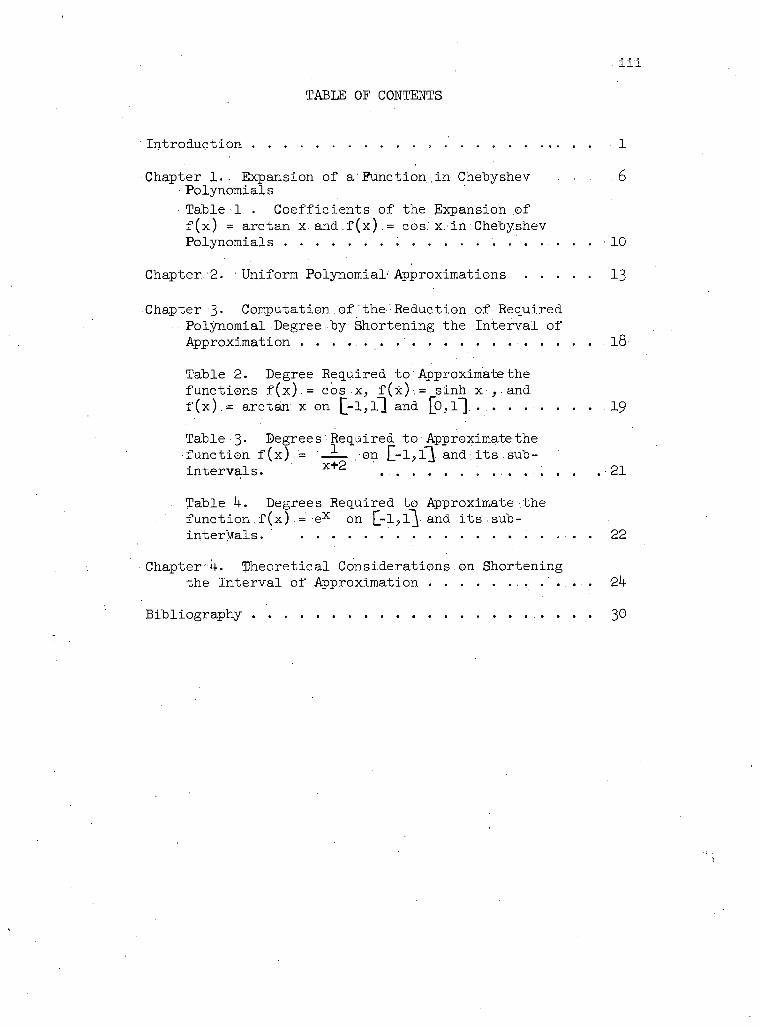
Ill TABLE OF CONTENTS
I n t r o d u c t i o n . . . . . . . . . . . . 1
Chapter 1.- Expansion of a'Function,in Chebyshev 6 Polynomials • Table 1 . C o e f f i c i e n t s of the Expansion of f ( x ) = a r c t a n x and f ( x ) = cos: x.-in Chebyshev Polynomials . . . . . . . . . . . . . . . 10
Chapter. 2. Uniform Polynomial' Approximations 13
Chapter 3- Computation.of the•Reduction of Required Polynomial Degree by-Shortening the I n t e r v a l of Approximation . . . . . . l8-
Table 2. Degree Required to.'Approximate the f u n c t i o n s f ( x ) . = cos x, f ( x ) , = s i n h x ^ a n d f( x ) . = a r c t a n x on £-l,l] and [b,l~]. ... .... . . • 19
Table :3- Degrees Required to'Approximate the f u n c t i o n f (x) -A- .en £-1,1^ and,its.sub-i n t e r v a l s . x + 2 . . 2 1
Table k. Degrees Required to Approximate .the f unction f ( x ) = e x on Q-1,1^ and i t s sub-i n t e r V a l s . 22
Chapter:k. T h e o r e t i c a l Considerations.on Shortening the I n t e r v a l of Approximation ... . . . ... . . . . . 2k
B i b l i o g r a p h y 30
i v
• ACKNOWLEDGEMENT
The author-wishes, to acknowledge h i s indebtedness, to Dr. T.E. H u l l , f o r
h i s p a t i e n t .guidance, i n f o r m u l a t i n g t h i s t h e s i s .
\To the s t a f f of the Computing Centre of the U n i v e r s i t y of B r i t i s h
Columbia,,the.author expresses h i s thanks. T h e i r e f f o r t s , made p o s s i b l e
the v e r i f i c a t i o n i n p r a c t i c e of t h e o r e t i c a l r e s u l t s .
F i n a l l y , the author thanks the N a t i o n a l Research C o u n c i l of Canada
f o r - t h e i r f i n a n c i a l support.
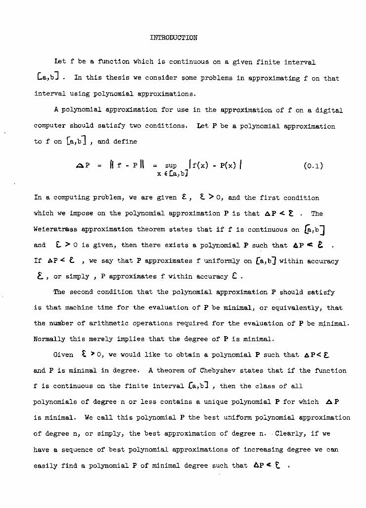
INTRODUCTION
Let f be a f u n c t i o n which i s continuous on a given f i n i t e i n t e r v a l
Ca,bl . In t h i s t h e s i s we consider some problems i n approximating f on th a t
i n t e r v a l u s i n g polynomial approximations.
A polynomial approximation f o r use i n the approximation o f f on a d i g i t a l
computer should s a t i s f y two c o n d i t i o n s . Let P be a polynomial approximation
to f on Cajb1 > and de f i n e
A P = f | f - P l l = sup |f(x) - P(x) / (0.1) x € Ca,b]
In a computing problem, we are given £ , Z. > 0, and the f i r s t c o n d i t i o n
which we impose on the polynomial approximation P i s th a t < E • The
Weieratrass approximation theorem s t a t e s t h a t i f f i s continuous on £a,b^J
and £. > 0 i s given, then there e x i s t s a polynomial P such t h a t AP < £
I f AP <• L , we say t h a t P approximates f u n i f o r m l y on £a,b]] w i t h i n accuracy
£. , or simply , P approximates f w i t h i n accuracy £ .
The second c o n d i t i o n t h a t the polynomial approximation P should s a t i s f y
i s t h a t machine time f o r the e v a l u a t i o n o f P be minimal, or e q u i v a l e n t i y , t h a t
the number of a r i t h m e t i c operations r e q u i r e d f o r the e v a l u a t i o n o f P be minimal.
Normally t h i s merely i m p l i e s t h a t the degree o f P i s minimal.
Given E > 0, we would l i k e t o o b t a i n a polynomial P such t h a t A P < £ .
and P i s minimal i n degree. A theorem o f Chehyshev s t a t e s t h a t i f the f u n c t i o n
f i s continuous on the f i n i t e i n t e r v a l La, , then the c l a s s of a l l
polynomials o f degree n or l e s s c o n t a i n s a unique polynomial P f o r which A P
i s minimal. We c a l l t h i s polynomial P the best uniform polynomial approximation
of degree n, or simply, the best approximation o f degree n. C l e a r l y , i f we
have a sequence of best polynomial approximations of i n c r e a s i n g degree we can
e a s i l y f i n d a polynomial P of minimal degree such t h a t AP < t. •
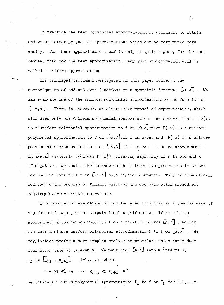
I n . p r a c t i c e the best polynomial approximation i s d i f f i c u l t to o b t a i n ,
and we use other polynomial approximations, which. can .be•• determined more
e a s i l y . For these approximations. A P i s only s l i g h t l y h igher, f o r the same
degree,.than f o r the best approximation. .Any, such approximation w i l l be
c a l l e d a uniform approximation.
The p r i n c i p a l problem .inves t i g a t e d i n t h i s paper concerns the
approximation of odd-and even f u n c t i o n s on a symmetric : i n t e r v a l C-a,a~3 . We
can evaluate one-of the uniform polynomial, approximations to • the f u n c t i o n on
[_-a,a"] . There i s , . however, . an ; a l t e r n a t i v e method of approximation, which
.also uses only, one•uniform'polynomial.approximation. We observe that, i f ' P(x)
i s a - uniform polynomial, approximation to f.on Co, al then P(-x) i s - a uniform
polynomial approximation to f, on £-a ,0~].if f i s even, and -P(-x) i s a uniform
.polynomial approximation to f on C-a,o]] i f f i s . odd. • Thus to .approximate f
on C-a,a1 we merely evaluate P|( \x\), changing s i g n . only.-if f i s . odd. and x
i f negative. We would, l i k e - t o know which.of these•two procedures, i s b e t t e r
f o r the e v a l u a t i o n of f on C-a^a"] on,a d i g i t a l , computer. This problem c l e a r l y
reduces to the problem of f i n d i n g which, of the two e v a l u a t i o n procedures
requires fewer a r i t h m e t i c operations.
-This problem of e v a l u a t i o n o f odd.and-even f u n c t i o n s • i s . a s p e c i a l case of
a problem of much grea t e r computational s i g n i f i c a n c e . I f we wish to
approximate a continuous, f u n c t i o n f on a f i n i t e • i n t e r v a l CAJD1 > we may
evaluate a s i n g l e uniform .polynomial approximation•P to f on [ a , b j . We
•may.-instead prefer-a-more complex e v a l u a t i o n procedure which can reduce
e v a l u a t i o n time c o n s i d e r a b l y . We p a r t i t i o n i n t o m i n t e r v a l s ,
I i .= £^Xj_ , xi+1~3 , i = l , ...m, where
We-obtain a uniform polynomial approximation P- t o f on.Ij_ f o r i = I , ...m.
a - x i x 2 • • • • < <. Xm+i = b
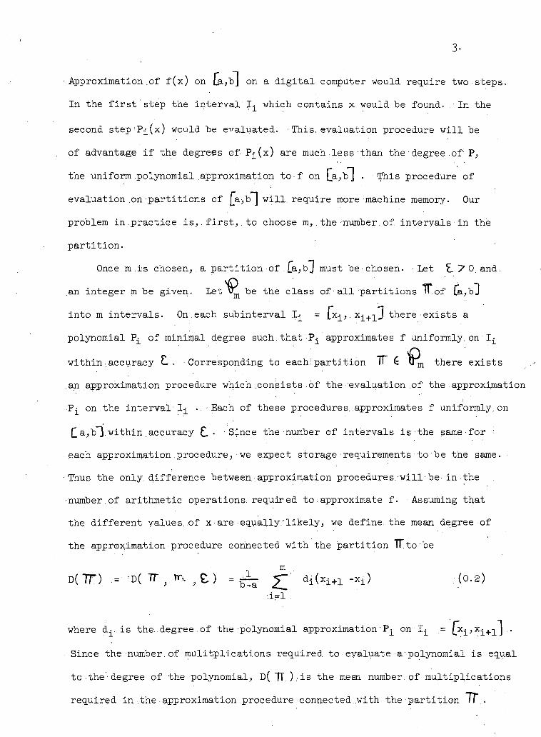
Approximation of f ( x ) on £a,b~| on a d i g i t a l computer would r e q u i r e two steps..
In the f i r s t . s t e p the i n t e r v a l 1 1^ which contains, x would be found... In the
second s t e p P j _ ( x ) would be evaluated. • This, e v a l u a t i o n procedure w i l l be
of advantage i f the degrees of Pj_(x) are much l e s s ' t h a n the • degree .of; P,
the uniform .polynomial approximation t o - f on Ca>b~] . This procedure of
e v a l u a t i o n .on p a r t i t i o n s of [a,b~] w i l l require-more machine memory. Our
problem .in . practice • i s , . f i r s t , . - t o choose m, , the -number. of. i n t e r v a l s i n the
p a r t i t i o n .
Once m i s chosen, . a p a r t i t i o n of , [a., b"] must be chosen. -Let £. 7 0. and.
an i n t e g e r m be given. L e t ^ ^ be the c l a s s of a l l p a r t i t i o n s IT of fa,bj
i n t o m i n t e r v a l s . On.each sub i n t e r v a l Ij_ .= [x^,, x +-[_^J. there e x i s t s • a
polynomial Pj_ of minimal degree such, t h a t P^ approximates f uniformly, on 1^
w i t h i n accuracy £. . Corresponding to e a c h : p a r t i t i o n there e x i s t s
.an approximation procedure which .consists of t h e - e v a l u a t i o n of the approximation
Pj_ on the interval'.Ij_ .. • Each of these procedures, approximates f uniformly, on
(2 a,b~J. w i t h i n , accuracy £.. Since the number of i n t e r v a l s i s the same f o r :
each .approximation .procedure, „• we-expect storage •requirements to be the same.
Thus the only, d i f f e r e n c e between,-approximation procedures.-will-be-in ,the
•number, of a r i t h m e t i c .operations, r e q u i r e d to •• approximate f. Assuming t h a t
the d i f f e r e n t values..of x a r e - e q u a l l y / l i k e l y , . we define, the mean degree of
the-approximation :procedure connected w i t h the p a r t i t i o n TTto be
m ,
D( TT) = -D( 7T , m. , e ) = ^ - d i ( x i + 1 - x i ) (0.2) 1=1 .
where d'.. i s the..degree .of the polynomial approximation 'Pj_ on: 1^ ,= f^iJ x±+i^] ••
Since the number.of m u l i t p l i c a t i o n s r e q u i r e d to - evaluate a polynomial i s equal
to the-degree of the -polynomial, D( "TT ) , i s the mean :number.of m u l t i p l i c a t i o n s
r e q u i r e d .in-.the - approximation procedure connected.with the p a r t i t i o n TT..
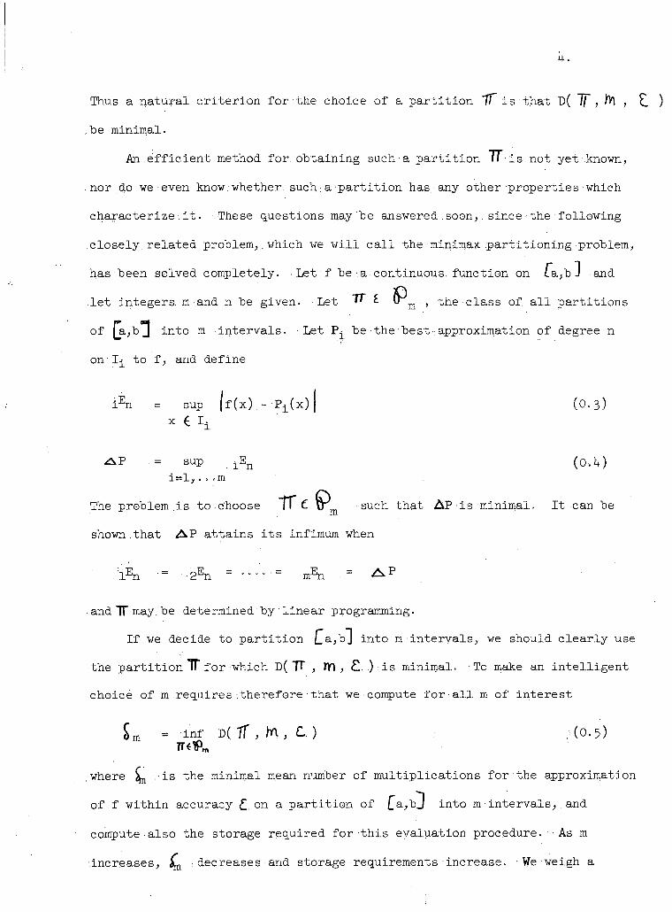
Thus a n a t u r a l c r i t e r i o n f o r the choice .of a p a r t i t i o n TT i s t h a t D( If , ft\ ,
he minimal.
An e f f i c i e n t method for. o b t a i n i n g .such a p a r t i t i o n 71 i s not yet .known,
nor do we. even know.whether, such :a p a r t i t i o n has any other p r o p e r t i e s , which
.characterize •. i t . These questions may be answered .soon, . since-the f o l l o w i n g
c l o s e l y , r e l a t e d problem,. which we w i l l c a l l the -minimax p a r t i t i o n i n g problem,
has been solved completely. • Let f be-a continuous, f u n c t i o n on /~a,bJ and
l e t i n t e g e r , » and n be given, rat TT £ P m , the c l a s 5 C a l l p a r t i t i o n s
of | ^ L,b^ i n t o m i n t e r v a l s . • Let be-the best-approximation .of degree n
o n l ^ to f,. and. define
i E n = sup ( f ( x ) . - P i ( x ) ( 0 . 3 ) x ^ T - i
= sup ^ (0,4) i = l , . . .m
The problem.is to.choose T T C Qm such.that A P • i s • minimal. I t can be
shown t h a t A P a t t a i n s i t s infimum when
l K n ' = 2 En " mEn —
andTTmay.be determined by l i n e a r programming.
I f we decide to p a r t i t i o n Ca,bj i n t o m i n t e r v a l s , . we should c l e a r l y . u s e
the p a r t i t i o n f o r which D( TT , 1Y\ , £..).• i s minimal. To make an i n t e l l i g e n t
c h o i c e , of m requires-.therefore t h a t we-compute f o r a l l m of i n t e r e s t
Sm = i n f D( TT , tn, t.) . ( 0 . 5 )
where ^ . i s the minimal mean number of m u l t i p l i c a t i o n s f o r the approximation
of f w i t h i n accuracy £ on a p a r t i t i o n of £a,bj i n t o m i n t e r v a l s , . a n d
.compute-also the storage r e q u i r e d f o r . t h i s e v a l u a t i o n procedure. • As m
inc r e a s e s , ^ . decreases and storage-requirements increase. - We weigh a
• '5-
decrease i n e v a l u a t i o n time against an.increased storage requirement i n
choosing m. Given £. >.0, we can choose, m s u f f i c i e n t l y l a r g e ' t h a t • a l l the
polynomial approximations would be constants • and", our e v a l u a t i o n procedure
would be a t a b l e • l o o k - u p ; t h i s would hardly.be•an e f f i c i e n t use of storage.
In Chapter 3 we give computed r e s u l t s r e l e v a n t to these problems.
Chebyshev.polynomials, on £-l,l] and the expansion of a f u n c t i o n . i n
Chebyshev.polynomials on £l,lj..are studied, in' d e t a i l , i n Chapter 1. An.
.important reason f o r t h i s study i s t h a t the methods, of o b t a i n i n g uniform
polynomial approximations depend on the p r o p e r t i e s , of expansions.in
• Chebyshev. polynomials, f o r t h e i r t h e o r e t i c a l j u s t i f i c a t i o n . • Further,. the
most u s e f u l of these methods, i s t r u n c a t i o n of. the expansion ,of. the-.(function
i n Chebyshev polynomials. Thus the computation of the c o e f f i c i e n t s of
the expansion of a f u n c t i o n i n Chebyshev polynomials, i s of great p r a c t i c a l
: importance,. and i s t r e a t e d . i n d e t a i l in.Chapter 1. At the end of Chapter.2
we - show how.the c o e f f i c i e n t s of the expansion of a f u n c t i o n i n Chebyshev
.polynomials can o f t e n be•used .to obtain.a good'estimate of AP f o r the
best uniform polynomial approximation.
I t i s o f t e n convenient to deal only w i t h approximation on the standard
i n t e r v a l f-l,l~J although sometimes we may f i n d , i t u s e f u l to d e a l w i t h
approximation on (0, 1~] a l s o . ; • By ' l i n e a r change - of v a r i a b l e we can . always
reduce the problem of uniform approximation on £a,b} to the problem .of
uniform approximation on a standard . i n t e r v a l . By using the standard
i n t e r v a l f-1, .il we need only, deal w i t h the•• Chebyshev polynomials, on

CHAPTER 1
EXPANSION OF A FUNCTION IN CHEBYSHEV POLYNOMIALS
F i r s t we summarize the pr o p e r t i e s , of the Chebyshev polynomials.which
we w i l l f i n d u s e f u l , l a t e r .
The k t h Chebyshev polynomial on [ r l , l j , T j £ ( x ) , ! i s d e f i n e d by
T ^ x ) = cos (k. arc cos x) - l * x i ' l (l»l)
From the a d d i t i o n formula f o r cosines • we ob t a i n the r e c u r s i o n . r e l a t i o n
T r + 1 (x) - 2 x T r ( x ) + T ^ U ) ,= 0 (1.2)
which, together w i t h the s t a r t i n g values
T 0 ( x ) .= 1 T-^x) .= x (1.3)
enables us t o express Chebyshev polynomials i n powers of x. Using ( l . 2 )
we can,show t h a t T k ( x ) i s a k t h degree polynomial and.that, i f k. i s .even
(odd)., so i s T k ( x ) . The values of T k ( x ) ; a t c e r t a i n . p o i n t s are of i n t e r e s t .
T k ( l ) . = 1 T k(:-1).= ( - l ) k T 2 k ( 0 ) . = ( - l ) k T 2 k + 1 ( 0 ) . = 0 (l.k)
We introduce n o t a t i o n which w i l l be used f r e q u e n t l y .
n 1 a j = -j + a l + •••• + S - l + ^ - 5 )
-J —u
t. 1 1 a i = !2. + a l +••••+ + f n (l -6) j=0 2 2
I f we wish to w r i t e powers of x i n terms of Chebyshev polynomials, we use
2k+l n k = ~^T I. ( 2 k + l ; ) T x ( x ) (1.8)
2 j=0 k-j d J

Frequently we f i n d the f o l l o w i n g t r a n s f o r m a t i o n u s e f u l
x = cos e Tk(x) = cos. k e - I ^ X ^ I oie^7r
The zeros of T n ( x ) (cos n, ©) are l o c a t e d at the n p o i n t s
cos ( 2 J - l ) - r r 2n (e,- = .(gJ -DTT. )
3 2n 1 3 " L> * *''n
(1 -9)
(1.1G)
The extremes of T n ( x ) (cos n O) ,alternate i n s i g n and are l o c a t e d at the
n+1 p o i n t s
" ~ ' j.= 0,1,...n . ( l . l l ) X . .= cos UL-• J
(ei .= -AIL. ) n n -'0
We have two o r t h o g o n a l i t y p r o p e r t i e s which are u s e f u l i n ..obtaining the
c o e f f i c i e n t s of an expansion i n Chebyshev polynomials.
1 T r ( x ) T s ( x ) d .
•1 41-x2
TT cos rG'cos sO d0 =
0
7f
JL 2
L 0
r = s = 0
r = s / 0 (1-12)
For 0 5 r ^-n, 0 i s i n we have
^ T 1 1 T k ( c o s i f . ) T s ( c o s i T ^ . ) =
• J=0
r 3=0
cos r j TT n cos s j TT
C n . r = s. = • 0
n 2
r.-= s / 0
r f s
(1-13)
We now consider expanding functions..in Chebyshev.polynomials on f - l , l j .
I f f ( x ) i s continuous and of bounded v a r i a t i o n . i n there i s an expansion
.of the form
(1.14) f(x)..« £ 1 c k T k ( x ) k=0
which converges u n i f o r m l y on . We w i l l show, i n Chapter 2 th a t uniform
polynomial approximations can be obtained most conveniently, by t r u n c a t i o n of

8.
( l . l U ) and we w i l l show t h a t the t r u n c a t i o n e r r o r bound AP f o r uniform
polynomial approximations can be computed easily."by. the use-of•formulas
i n v o l v i n g the c o e f f i c i e n t s of the expansion. Thus the problem of computing
the c o e f f i c i e n t s i s an :important p r a c t i c a l problem and we consider i t i n
d e t a i l .
From (l. 1 2 ) we ob t a i n the r e l a t i o n
c = 2 (~ T k ( x ) d x = g f (cos ©) cos ke d0 ( l - 1 5 )
C l e a r l y i f f i s even (odd) the odd.(even) c o e f f i c i e n t s w i l l v a nish because
T k(.x) i s even (oddX.if k i s even (0dd). E x p l i c i t expressions f o r the c o e f f i c
i e n t s C k of many, common functions-have been obtained using t h i s r e l a t i o n . In
the best c o l l e c t i o n [j3;.p.2l4~] of such r e s u l t s we f i n d a formula f o r the
c o e f f i c i e n t s C k of f ( x ) . = a r c t a n x on Q l , l J which we us e - i n the s p e c i a l form
. ? a J + 1 . . . 2(-l)' ( iS-lf^1 .o ( 1 . 1 6 )
2 j + l
.to prepare Table 2 i n Chapter 3. In general:(l. 1 5 ) cannot be e a s i l y i n t e g r a t e d
and use of the f o l l o w i n g methods i s p r e f e r a b l e to numerical i n t e g r a t i o n of
(1.15)-
^k n m a y - b e used as an.approximation,to C k , k-= 0, ....n,•where
= - V 1 1 f ( c o s JJL.) cos iKTf (1-17)
From an extension of (1.13) we o b t a i n an exact expression f o r tf, . K. y n
^ k , n " ..= . ZT c2mh"+k + ^ c2nm-k m=0 i:m=l ( l . l 8 )
•Ck ; + G 2n-k + C2n+k + C Un-k + CUn+k + C 6n-k + "C6n+k
. 9-
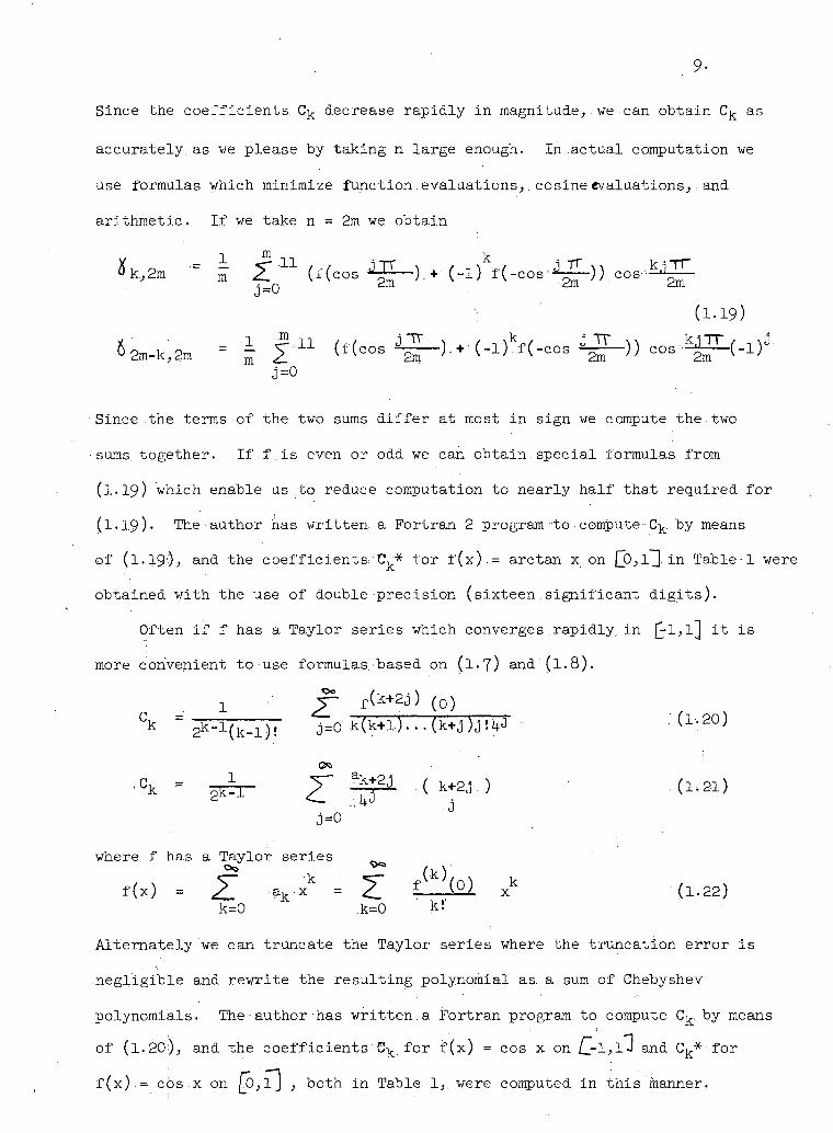
Since the coefficients. C k decrease rapidly i n magnitude,,we can obtain C k as
accurately, as we please by taking n large enough. In actual computation we
use formulas which minimize function.evaluations,. cosine evaluations, and
arithmetic. I f we take n •= 2m we obtain
*k,2m. = } Z 1 1 ( f ( c o s J J - ) . + - ( - l ) k f ( - c o s - ^ ) ) . c o B - ^ ^ = 0 2m v ' s -2m 2m
(1-19)
62m-k,2m - I I 1 1 ( f(coB^). + ( . l ) k f ( - c o B . ^ ) ) . c o s - ^ < - l ) J -
• Since :the terms of the two sums d i f f e r at most i n sign we,compute the two
sums, together. I f . f . i s even or odd we can obtain. special formulas from
(l . l 9 ) which enable us.to reduce computation to nearly half that required f o r
( l . l 9 ) . The - author, has written, a Fortran 2 program to compute - C k by. means
of (1.190; and the c o e f f i c i e n t s C .* for f(x),= arctan x on j j ) , l 3 i n Table-1 were
obtained with the use of double precision (sixteen .significant d i g i t s ) .
Often i f f has a Taylor series, which converges.rapidly, i n f j - l , l ] i t i s
more convenient to-use formulas, based on (1.7) and (1.8).
1 f ( ^ g j ) (0)
° k ~ 2 k " 1 ( k - l ) ! J = ° k(k+l)...(k+j) ti!l | 0 • C.1:20)
<ck = p r r - Z ( k+2J } (1'21)
• 3 3=0
where f has a Taylor series °* (k)
f(x) = Z a k,x k = 2" £ _ M x k (1.22) k=0 k=0 ^ !
Alternately we can truncate the Taylor series where the truncation error i s
neg l i g i b l e and rewrite the resulting polynomial as. a sum of Chebyshev
polynomials. The • author has written, a Fortran program to compute • C.. by means
of (1.20), and the c o e f f i c i e n t s C k for f(x) = cos x on LT-1>1^ and C k* for
f(x).= cos x on £o,l~] , both i n Table 1,. were computed i n t h i s manner.
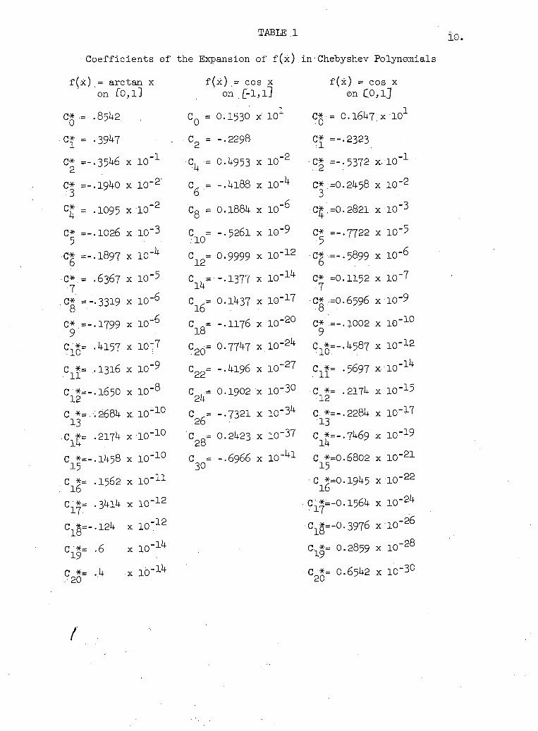
TABLE 1
C o e f f i c i e n t s of the Expansion of f ( x ) . i n Chebyshev Polynomials
f ( x ) = arct a n x f ( x ) = cos x f ( x ) = cos x on f O , l ] on.£-l,ll on C 0 , l j
,8542. C 0 = 0.1530 X 1 0 1 C* = 0.l647.x 10 1
c ! = • •3947 C 2 = -.2298 c* =-.2323
c* =-. 2
•35^6 X 10" -1 C 4 =
0.4953 X 10' -2 -C* =-.5372 X IQ" 1
.1940 X 10" -2: V -.4188 X 10' -4 c* =0.2458 3
X IQ" 2
,1095 X 10' -2 c 8 = 0.1884 X 10' -6 •C7*. =0.2821 X 10" 3
c* =-. 5
.1026 X 10' -3 c •= .10
-.5261 X 10' -9 c* =-.7722 X 10-5
°? -.1897 X 10" -k 0.9999 X •10" -12 •c* =-.5899 X 10 " 6
c*.= . •T
.6367 X 10' -5 °lk~ -.1377 X 10' -14 c* =0.1152
7 X 10-T
C 8 = -.3319 X 10" -6
C16" 0.1437 X 10' -17 -c* =0.6596 X io - 9
c* 9
•1799 X 10' -6 C 1 8 -
-.1176 X 10' -20 C* =-.1002 9
X I Q " 1 0
C '*= . 10 •4157 X 10" -1 °20" 0.7747 X 10' -24 ^ = - . 4 5 8 7 X l O - 1 2
c *= . 11
.1316 X 10' -9 -.4196 X 10' -27 cx*= .5697 X io-lk
c •*=-. 12
.1650 X 10' -8 O.1902 X 10" -30 c *= .2174 12
X 10-15
c *=.• 13
C l t = •
.2684 X 10' -10 -.7321 X 10" -34 C *=-.2284 13
c *=-.7469 14
X 1 0 - " c *=.• 13
C l t = • .2174 X •10" -10 0.2423 X 10' -37
C *=-.2284 13
c *=-.7469 14
X l O " ^
c *=-15
.1458 X 10' -10 c = 30
-.6966 X 10' - 4 l C *=0.6802 15
X 1 0 - 2 1
C i 6 = .1562 X 10' -11 c *=o.i945
16 X 1 0 - 2 2
C 1 7 = .3414 X 10' -12 C^ - 0 . 1 5 6 4 X 1 0 - 2 4
Cl§=- .124 X 10' -12 0^=-0.3976 X 1 0 - 2 6
c i r .6 X 10' -14 c^= 0.2859 X 1 0 - 2 8
c 2 0 -.4 X 10 -14 • ( V * = O.6542
.20 ^ X 10-30
f
.•11.
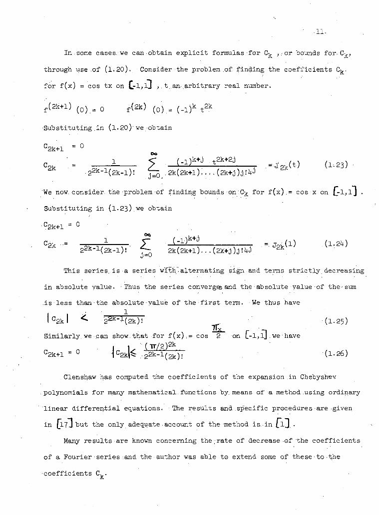
In some cases we c a n ; o b t a i n e x p l i c i t formulas f o r C k ,. or bounds f o r - C k ,
through use .of (1.20).. Consider the problem .of. f i n d i n g the c o e f f i c i e n t s Ck.
f o r f (x) .= cos t x on C-1;J t,an-,arbitrary r e a l number.
f ( 2 k + 1 ) (o).= o f ( 2 k > (o).= ( - i ) k t 2 k
S u b s t i t u t i n g i n ( l . 2 0 ) we ob t a i n
C2k+1 = 0
c 2 k . _ ! — £ ( . i ^ . t ^ ; ( t ) ( i , 2 3 )
- 2 2 k - 1 ( 2 k - l ) ! ^5 .2k(2k+l)....(2k+j)a.'M " .
'We now. consider- the -problem of f i n d i n g bounds on Ck. f o r f (x) ,. = cos x on []-l,l"3
S u b s t i t u t i n g i n (1 .23) we o b t a i n C2k+1 = 0
_ i . T ( - l ' ) k + J = . J p k ( l ) (1.24) c 2 k
2 2 k _ 1 ( 2 k - l ) ! ' ^ 2k(2k+l) . . . (2k+j ) j!i+J
T his s e r i e s , i s a s e r i e s w'ith'alternating s i g n .and terms s t r i c t l y decreasing
i n absolute value. Thus the s e r i e s converges-and. the absolute value of the-sum
i s l e s s than the-absolute value of the f i r s t term. We thus have I 1
| C 2 k | < .-2«iK-±(2k)! (1-25)
S i m i l a r l y , we can show.that f o r f ( x ) . = cos 2 on L-l>lJ•we - have I 1 " (-n-/2) 2 k
C2k+1 = 0 | c 2 k | ^ - 2 2 k " 1 ( 2 k ) ! (1-26)
. Clenshaw has computed the c o e f f i c i e n t s of the expansion i n Chebyshev
polynomials f o r many mathematical.functions by. means of a method usi n g o r d i n a r y
l i n e a r d i f f e r e n t i a l equations. The r e s u l t s a n d . s p e c i f i c procedures are given
i n (17"].but the only adequate-account of the method i s . i n £V] •
Many r e s u l t s are known concerning t h e ; r a t e of decrease of the c o e f f i c i e n t s
of a F o u r i e r series-.and the author was • able to extend some of these to the
c o e f f i c i e n t s C ..
• 12.
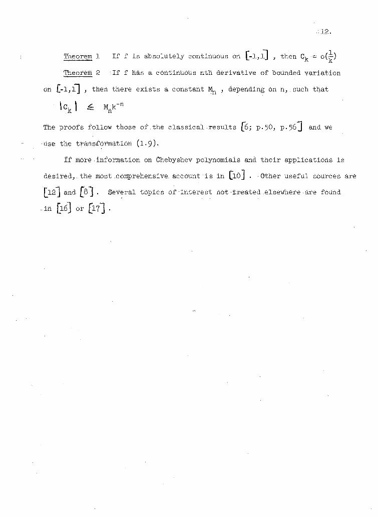
Theorem 1 I f f i s a b s o l u t e l y continuous on £-l,l] , then C . •= o(g-)
'Theorem 2 I f f has a continuous nth d e r i v a t i v e - o f hounded.variation
on £-1,1~] , then there e x i s t s a constant , depending on Xi, . such t h a t
\c, I ^ M k' n
k 1 n
The p r o o f s f o l l o w those of .the c l a s s i c a l r e s u l t s [6; p. 'pO, p. 56 ] and we
use the tr a n s f o r m a t i o n (1-9)-
I f more i n f o r m a t i o n on Chebyshev polynomials and t h e i r a p p l i c a t i o n s i s
d e s i r e d , .the most comprehensive, account i s i n Cioj • • Other useful, sources are
£l2*] and j*8~J . Se v e r a l t o p i c s of i n t e r e s t n o t ' t r e a t e d .elsewhere-are found
i n [ l6] or [ I ? ] •

13-
• " • :'; • CHAPTER 2
UNIFORM POLYNOMIAL APPROXIMATIONS
Let f(x) be continuous on [a.,b] and l e t P be a polynomial of degree n or
less such that o'(x),
$(x),= f(x)-P(x) ..... ... ( 2 . 1 )
attains i t s greatest absolute value on at least n+2 points i n [a.b^j and i s
alternately, positive and negative on these points. Then P i s .the best uniform
polynomial approximation of degree n. A class of methods c a l l e d the direct
methods enables us to compute best approximations by constructing a polynomial
with t h i s alternating property. Fras'er and Hart [_2~j give the relevant theory,
one such method, and references to a l l . s i g n i f i c a n t l i t e r a t u r e . The direct
methods require double precision and very extensive computation. For t h i s reason
i f f had a Taylor series converging rapidly, i n £ - 1 , i j • Maeh-ly. preferred to use
his combined method [iVJ to obtain a best approximation. Hornecker
has obtained formulas which usually, enable us to compute best - approximations
from the c o e f f i c i e n t s Ck- 1
There i s also.a class of methods, the trigonometric interpolations,
which i s closely, related to truncation of an-expansion i n Chebyshev polynomials.
Two methods described i n ^ 5 T a r e Lagrange•interpolation.at.the zeros of the
n + 1 st Chebyshev. polynomial and ..best f i t t i n g a polynomial of degree n at the
extrema of the n + 1 st Chebyshev polynomial. The l a t t e r i s used .frequently, to
start the direct methods • Related methods are described i n .
The most convenient method i n practice for obtaining a uniform polynomial,
approximation i s truncation of the expansion i n Chebyshev polynomials.
We obtain an n th degree approximation
S n(x) .= ^ T 1 C kT k(x) (2.2)
k=0
1 4 .
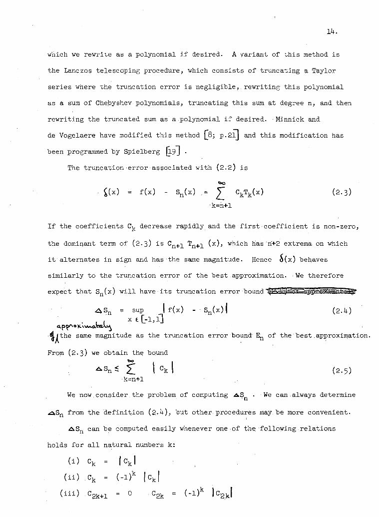
which we r e w r i t e as a polynomial i f d e s i r e d . A v a r i a n t of t h i s method i s
the Lanczos t e l e s c o p i n g procedure, which c o n s i s t s of t r u n c a t i n g a Tayl o r
s e r i e s where the t r u n c a t i o n e r r o r i s n e g l i g i b l e , , r e w r i t i n g t h i s polynomial
as.a sum of Chebyshev polynomials, t r u n c a t i n g t h i s sum at degree n, and then
r e w r i t i n g the truncated.sum as a polynomial i f d e s i r e d . Minnick and
de Vogelaere have modifi e d t h i s method (j8;.p .2l] and t h i s m o d i f i c a t i o n has
been programmed by S p i e l b e r g \l9~] •
The t r u n c a t i o n e r r o r a s s o c i a t e d w i t h (2.2) i s
£(x) = f ( x ) - S n ( x ) ,= £ C k T k ( x ) (2.3)
k=n+l
I f the c o e f f i c i e n t s C k decrease r a p i d l y and the f i r s t . c o e f f i c i e n t i s non-zero,
the dominant term of (2.3) i s Cn+-j_ Tn+-j_ ( x ) , which has ri+2 extrema on which
i t a l t e r n a t e s i n sign and has the same magnitude. Hence S(x) behaves
s i m i l a r l y to the t r u n c a t i o n e r r o r of the best approximation. - We th e r e f o r e
expect t h a t S n ( x ) w i l l have i t s t r u n c a t i o n p-i-i-m- ••hnnri - ^ ^ V ^ ^ t ^ p j ^ ^
^ S n = sup I f ( x ) - S n ( x ) | (2.k)
^ t h e same magnitude as the t r u n c a t i o n e r r o r bound ^ o f the best.approximation.
From (2.3) we ob t a i n the bound
^ s n ^ £ lCkl (2.5) k=n+l
We now.consider the problem of computing ^ S n • We can.always determine
^aSn from the d e f i n i t i o n (2 .4) , but other procedures may be more convenient.
A S n can be computed e a s i l y whenever one of the f o l l o w i n g r e l a t i o n s
holds f o r a l l n a t u r a l numbers k:
( i ) C k = | c k |
( i i ) c k = ( - i ) k | c k |
( i i i ) c 2 k + 1 = 0 C 2 k = ( - i ) k ) c 2 k i
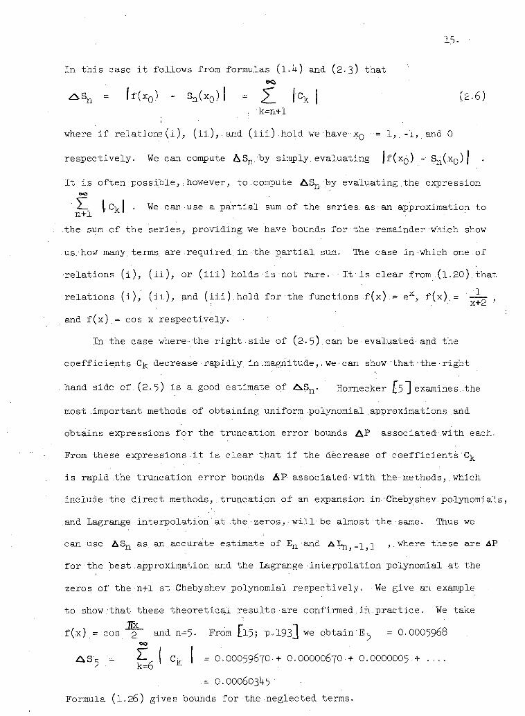
In t h i s case i t f o l l o w s from formulas (.1.4) and (2.3) that
^Sn = | f ( x 0 ) - S n ( x 0 ) | = |"Ck j (2.6) k=n+l
where.if r e l a t i o n s ( i ) , ( i i ) , a n d ( i i i ) . h o l d we have X Q = 1 , - 1 , and 0
r e s p e c t i v e l y . We can compute AS n.'by.simply, e v a l u a t i n g Jf(.XQ) -• Sn(xo) | I t i s o f t e n p o s s i b l e , ; however, t o . compute AS n."by e v a l u a t i n g the expression
$1 { C k| . We can use a p a r t i a l sum of the series, as an.approximation to
the sum of the s e r i e s , p r o v i d i n g we have bounds f o r the remainder which show
. us. how many, terms, are required, i n the p a r t i a l sum.. The case i n which one.of
• r e l a t i o n s ( i ) , ( i i ) , or ( i i i ) h o l d s - i s not r a r e . I t - i s c l e a r from .(1.20).that
r e l a t i o n s ( i ) , ( i i ) , and ( i i i ) , h o l d f o r the f u n c t i o n s - f ( x ) . = e x , f ( x ) , = ' y
and f(-x).= cos x r e s p e c t i v e l y .
i I n the case-where-the-right.side-of (2.5).can be-evaluated and.the
c o e f f i c i e n t s C . decrease r a p i d l y , i n ..magnitude,, we can . show th a t - the • r i g h t
hand side of. (2. 5) i s a good estimate of A.S n. Hornecker [ 5 ~] examines, the
most .important methods of o b t a i n i n g uniform .polynomial .approximations..and
obtains expressions f o r the t r u n c a t i o n e r r o r bounds A P ass o c i a t e d - w i t h ,each.
From these expressions i t i s c l e a r - t h a t . i f the decrease-of c o e f f i c i e n t s C k
i s r a p i d the t r u n c a t i o n e r r o r bounds A P as s o c i a t e d w i t h the-methods,.which
in c l u d e the d i r e c t methods, t r u n c a t i o n of an expansion i n Chebyshev.polynomials
and Lagrange i n t e r p o l a t i o n at the zeros,- w i l l / b e almost the same. Thus we
can use A S n as an,accurate estimate of E n.and. A L J ^ . ^ ^ ,. where these are AP
for. the best .approximation. and the L a g r a n g e - i n t e r p o l a t i o n polynomial, at the
zeros of the n + 1 s t Chebyshev polynomial r e s p e c t i v e l y . We give an example
to show t h a t these t h e o r e t i c a l r e s u l t s are c o n f i r m e d . i n . p r a c t i c e . We take
f(-x).= cos 2 a"-11 n = 5 - From Ll-5.; P» 193J we o b t a i n = O.OOO5968
A S c = 21 ( C-k. I = 0,00059670.+ 0.00000670 + 0.0000005 + ••»• -> • k=6
.= 0.0006034.5 Formula (I..26) gives bounds for. the neglected.terms.
In t h i s example the s l i g h t decrease i n truncation error bound by
using the best uniform approximation. instead, .of. the. truncated ..expansion , i n
Chebyshev polynomials i s not of p r a c t i c a l significance. • Kogbetliantz (jj
discusses t h i s matter i n more d e t a i l with•another, example.
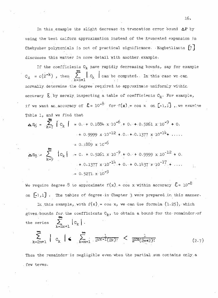
I f the c o e f f i c i e n t s C k have rapidly, decreasing bounds,., say. for example
Cv = 0(2"^) , then ^ |-.Cv | can.be computed... • In. t h i s case we can k=n+.l
normally, determine the degree required .to approximate uniformly within
accuracy £.. by merely, inspecting a table of co e f f i c i e n t s C k.•For example,
i f we want an .accuracy. of £= 10-® f o r f (x) ,=• cos x on C-l>l"3 > - w e examine
Table 1, and.we f i n d that
^Sg,= , . J ^ I C k I = 0. • + . 0.1.884 x l O .+ 0. •+ O.526.I x .10"9 + 0.
00
= 21 |c k I - 0. + O.526::. x 10 " 9 + 0 + C.9999 r l C ' 1 2 + C.
•+ 0.9999 x - 1 0 " 1 2 +.0..+.0.1377 x -10" 1 4 +
•= 0.1889 x 1 0 - 6
A S 8
k=9 + .0,1377 x l G ~ i l + + 0. + 0.1.437••x'--10"17.- +
0..5271. x -10" 9
We require degree 8 to approximate f(x).= cos x within accuracy C.= 1 0 - 8
on [ j l , l j . The tables of degree.in Chapter 3 were prepared .in t h i s manner.
In .this example,, with f(x).= cos x, we can.use formula (.1.25), which
gives, bounds for. the c o e f f i c i e n t s C k, . to obtain a bound for the - remainder-of 00
the series ^1 | C v I • k=2m+.l '
.k=Ln I C k I * .kS+l - 2 ^ - i ( 2 k ) - < .2^(2m+2)'. . (2.7)
Thus the remainder i s negligible even when the p a r t i a l .sum contains only a
few terms.
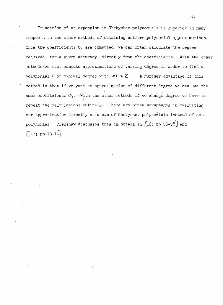
Truncation of an .expansion:in.Chebyshev.polynomials-• i s s u p e r i o r i n many
respects t o the other methods of o b t a i n i n g uniform .polynomial approximations.
Once the c o e f f i c i e n t s C k are computed,. we can o f t e n c a l c u l a t e the degree
r e q u i r e d , f o r a given accuracy, d i r e c t l y , from the c o e f f i c i e n t s . With the other
methods we must compute approximations o f v a r y i n g degree i n order to find.,a
polynomial P of minimal degree w i t h < £. . A f u r t h e r advantage of t h i s
method i s .that i f we-want an approximation of. d i f f e r e n t degree --we can use .the
same .coefficients-Cv_. With the other methods- i f we change degree we have to
repeat the c a l c u l a t i o n s e n t i r e l y . There..are o f t e n advantages •-in e v a l u a t i n g
our approximation d i r e c t l y as a sum of•Chebyshev.polynomials-instead of as a
polynomial. Clenshawrdiscusses t h i s in. d e t a i l ; i n £l6; .pp.76-78*! and
C 1 7 ; .PP. 1 3-ih] •
18.
CHAPTER 3
COMPUTATION. OF THE REDUCTION. OF "REQUIRED POLYNOMIAL DEGREE BY SHORTENING THE INTERVAL OF:' APPROXIMATION
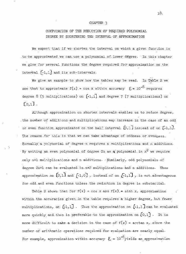
We expect t h a t i f we • shorten.the i n t e r v a l on which a given f u n c t i o n i s
to>be approximated.we can.use a polynomial .of. lower -degree. In t h i s chapter
we give f o r s e v e r a l f u n c t i o n s the degree r e q u i r e d f o r approximation on.the
i n t e r v a l Q-l,ij.and.its s u b - i n t e r v a l s .
We give, an . example to show. how.the t a b l e s may be read. In'Table 2. we
see t h a t to . approximate f ( x ) , = cos. x w i t h i n accuracy £j = 10"® . r e q u i r e s
degree 8 (5 m u l t i p l i c a t i o n s ) on £-l,l] and.degree 7 ( 7 . m u l t i p l i c a t i o n s ) on
Lo,il . Although, approximation on .shorter, interval's enables us t o reduce degree,
.the number of additions,.and m u l t i p l i c a t i o n s - m a y : increase i n the case :of an odd
or even, f u n c t i o n approximated on , the half.. i n t e r v a l (p, 1~\ i n s t e a d of on ( ~ - l , l J .
The reason .for t h i s , i s t h a t we-can take advantage of oddness or evenness.
-Normally a polynomial of degree-n r e q u i r e s n m u l t i p l i c a t i o n s and n a d d i t i o n s .
•By w r i t i n g an even polynomial of degree-2n as a;.polynomial, i n x 2 we-require
only, n+1 m u l t i p l i c a t i o n s and n a d d i t i o n s . • S i m i l a r l y , . odd polynomials of
degree 2n+l can be evaluated.in.n+2 m u l t i p l i c a t i o n s and n a d d i t i o n s . -Thus
approximation .on (o,l"3.and £-l,0~3 ,. i n s t e a d of on /-l,lD ,. i s • not advantageous
f o r odd.and even.functions unless the r e d u c t i o n i n degree i s s u b s t a n t i a l .
Table 2 shows th a t f o r f ( x ) = cos x and f ( x ) , = s i n h ; x,. approximation ;'
w i t h i n the accuracies given ; i n the t a b l e - r e q u i r e s a higher degree,,but fewer
- m u l t i p l i c a t i o n s , . on £l,lj • Thus the approximation on [-1, l l can be evaluated
more q u i c k l y and.thus i s p r e f e r a b l e - t o the approximation on £b,l3 . I t i s
more d i f f i c u l t t o make a d e c i s i o n i n the case of f ( x ) , = a r c t a n x,.since the
number of a r i t h m e t i c operations r e q u i r e d ..for e v a l u a t i o n , are n e a r l y equal.
For example, approximation w i t h i n accuracy £./= 1 0.^yields an approximation

19 ••
TABLE 2
d k = degree r e q u i r e d to approximate f ( x ) on the appropriate i n t e r v a l w i t h i n accuracy £ = 10~k
mk = number of m u l t i p l i c a t i o n s r e q u i r e d to evaluate the approximation of accuracy £ = 10~k
k :. f ( x) = cos x f ( : x).= s i n h x f ( : K ) , = a r c t a n x k
c- Co,il C-i,i1 C - l , l l foil mk 4k % = d k
'i m k d k mk= d k m k d k mk= d k
1 2 2 l .1 .1 1 1 .1 . .1 :1
.2 2 2 2 3 3 2 3 3 .2 2
3 3 .1+ 3 3 3 •3 ,4 •5 k 3 k •3 k h •5 .4 •5 •7 5 %
5 6 •k - ,k 5 5 7 l l 6 5 6 6 5 .5 7 5 . :8 •13 7 .6 7 5 .8 6 5 7 •6 9 15 9 7 ?8 5 8 7 •6 •9 7 10 17 . io 8
9 5 .8 7 6 •9 -7 .12 21 12 9 10 6 • 10 8 6 9 8 13 23 13 10
i l 6 10 9 •7 l l 9 ,1k 25 . 15 :11 12 7 .12 9 .7 . l l 9 15 .27 . 16 •12
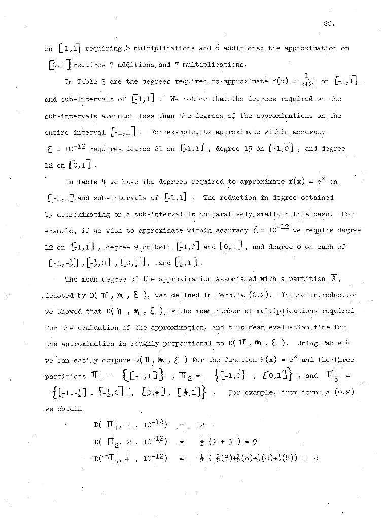
on [-1, l ] . r e q u i r i n g .8 m u l t i p l i c a t i o n s and. 6.additions;.the approximation.on
£b,l"J r e q u i r e s 7 a d d i t i o n s , and 7 m u l t i p l i c a t i o n s .
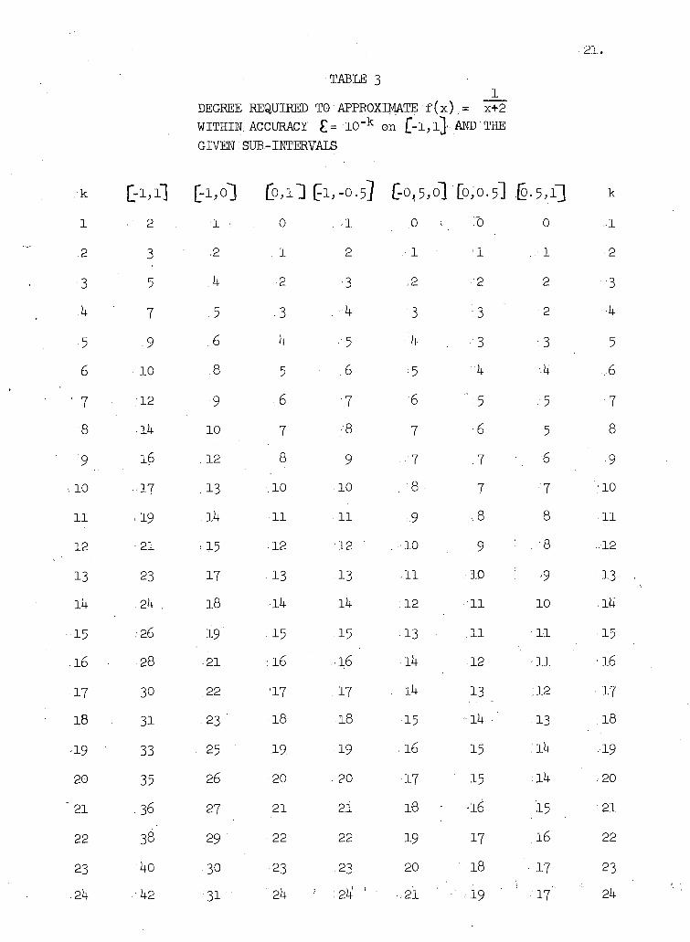
In Table 3 are the degrees r e q u i r e d .to • approximate • f ( x ) ,= ^ 2 on
and s u b - i n t e r v a l s of [^J-^ ' We n o t i c e that, the degrees r e q u i r e d on the
s u b - i n t e r v a l s are; much:less than the degrees of the.approximations on.the
e n t i r e i n t e r v a l £-1., l ] . For example, ;to :approximate w i t h i n ,accuracy
£ = 10 -- 1-2 r e q u i r e s degree 21 on G-l,ll , degree I'-y on £-l>0~] , and degree
12 on [0,1~[ .
In Table k we have the degrees, required, to approximate f(x)..= e x on
Q - l , l ~ ] ; a n d s u b - i n t e r v a l s of [V l , l j • The re d u c t i o n i n degree•obtained
by approximating on a s u b - i n t e r v a l ; i s , comparatively, small; i n . t h i s case. For r -12
example,. i f we wish to approximate wit h i n . a c c u r a c y c - 10 we re q u i r e degree
12 on fj-l, l"] ,. degree 9 -on "both £-l,o"J.and £ o , l j [ , and degree 8 on each of
C-l , -£ l ,[-h,0] , l0,f], .and ft,l}.
The mean degree of the approximation a s s o c i a t e d . w i t h ,a p a r t i t i o n TT,
. denoted by D( TT , 1A , £ ), was defined, i n ..formula (0; 2) In.-the i n t r o d u c t i o n
we showed t h a t D( TT , ft\ , £ ).is. the mean number, of m u l t i p l i c a t i o n s r e q u i r e d
f o r the e v a l u a t i o n . of. the approximation, and thus mean evaluation,time f o r .
the approximation,is roughly p r o p o r t i o n a l to D( TT• } W\ } £. ). Using.Table : k
we can e a s i l y compute D( IT, h\ , £ ) f o r the f u n c t i o n f !(x) ,= e X and the three
• p a r t i t i o n s
jjjl,-^] , [ - l b 0 ! •> L°>h3 > Li'1!}" • For example,. from .formula (0.2)
we ob t a i n
•p( 7T 1 V 1 , 1 0 " 1 2 ) ,= 12 ,
j)( ]T 2, 2 , I O ' 1 2 ) ,= (9 + 9 ).= 9
D( TT 3, L , 1 0-I 2) = . - \ (i(8 . )4(8 )4 , (8 )4(8)) ,= 8-
21.
TABLE. 3 1
DEGREE REQUIRED TQ'APPROXIMATE f ( x ) , = • x+2
WITHIN. ACCURACY £= 1 0 _ k.on £"-l,l}-ANDTHE GIVEN'' SUB-INTERVALS
[-1,1] C-i,ol (PA! f l , -O.5J C-0,5,0] [0,0. 5] [ 0 . 5,l] k
1 2 •1 .: 0 -1 ,0 v ~0 .0 ..1
.2 3 .2 . 1 2 .- 1 • 1 ..• 1 •2
3 5 .4 2 •3 .2 ••'2 2 3
,4 7 . .5 :3 •4 3 :3 •2 •4
•5 • 9 ,6 4 5 k 3 .3 5
6 10 .8 5 .6 •5 4 '•4 ,6
' 7 . 12 9 .6 '7. 6 ' 5 5 •7 8 -ik 10 7 .8 7 •6 5 8
9 16 . 12 8 9 7 .7 6 9
-. 10 -17 . 13 .10 10 . 8 • 7 :7 .'10
n 19 . .14 ,11 11 .9 ,8 8 11
12 - 21 -15 • 12 12 ' .-10 9 • . "8 .12
13 .23 17 A 3 . 13 ,1.1 10 • 9 -13
Ik 2k . 18 -14 14 ,12 l l 10 .14
• 15 .26 19 15 15 13 l l : 11 • 15
16 • •28 • 21 :16 •16 :l4 12 11 16
•17 . 30 .22 '17 17 . 1 4 13 ;12 17
18 31 • 23 " 18 18 •15 14 -13 .18
-19 33 • 25 19 19 .16 15 .14 19
20 35 26 20 20 •1.7 15 ' :14 , 20
- 21 36 27 21 21 .18 - •16 15 •21
22 38' 29 • 22 22 19 17 .16 22
23 .40 30 23 23 20 .18 ' 17 23
2k 42 ; 3 l 24 24 f ' 21 ' •' : 19 17" 24
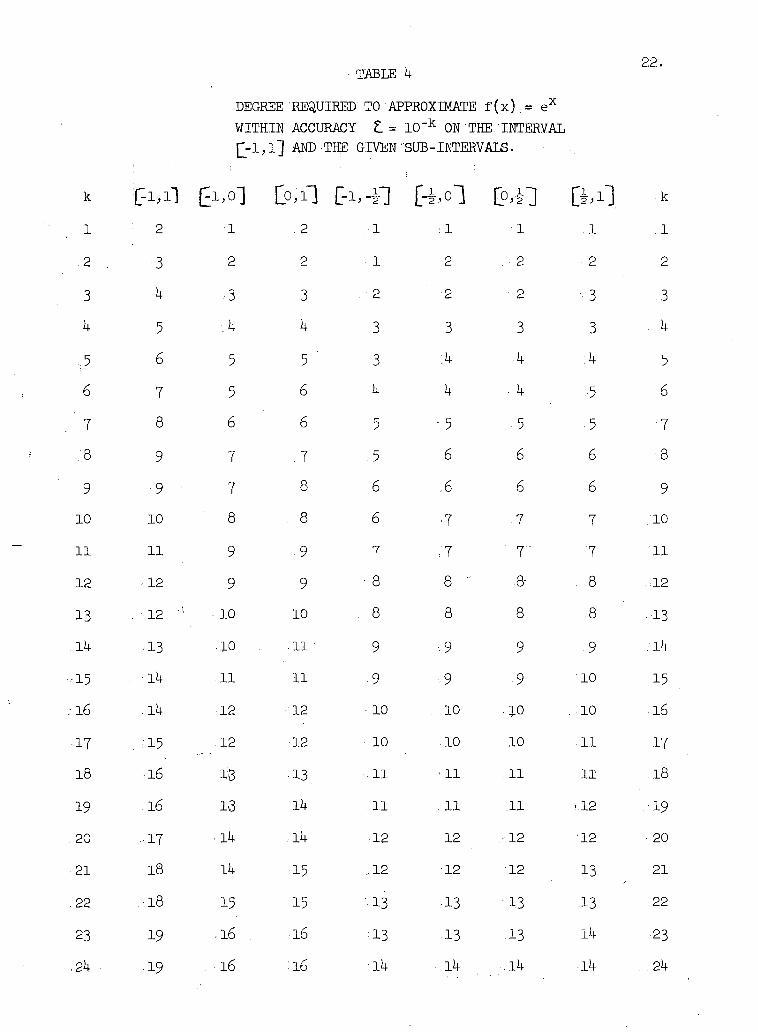
TABLE 4 22.
DEGREE REQUIRED TO APPROXIMATE f ( x ) , = e x
WITHIN ACCURACY t= 10"k ON THE. INTERVAL Q-l,l} AND THE GIVEN SUB-INTERVALS.
k foil Ml [-i,o~] EMI k
1 2 • i . 2 i : 1 i . 1 1
.2 3 .2 2 • i 2 . 2 2 2
3 k 3 3 . 2 •2 •2 •••3 3 4 5 .4 4 3 . 3 3 3 . 4
,5 . 6 5 5 ' 3 ;4 4 4 5
6 7 5 6 4 4 4 5 6
7 8 6 6 5 • 5 5 5 7
.'8 9 .7 . 7 . 5 6 6 6 8
9 9 7 8 6 .6 6 .6 9
10 •10 8 8 .6 •7 7 7 .10
i l . . l l 9 9 7 /7 " 7 " '7 l l
12 -12 9 9 8 8 - 8- . 8 .,12
13 . 12 10 10 . 8 8 8 .8 13
14 13 •10 • 11 - 9 ••9 9 9 .14
15 • :1k l l 11 9 • 9 9 10 15
16 .Ik ,12 . 12 • 10 . 10 • 10 . 10 16
17 . -15 . 12 12 • 10 • 10 10 .11 ' 17
18 16 13 •13 • 11 • l l . n i i .18
19 .16 13 14 , 11 : 11 : . l l .• 12 •19
20 •17 14 14 •12 •12 •1.2 12 . 20
21 18 14 15 ;12 12 12 13 21
22 .18 15 15 13 •13 13 13 .22
23 19 -16 . 16 13 13 13 14 23
2k • •19 . 16 :i6 14 • 14 :l4 ,14 .24
23.
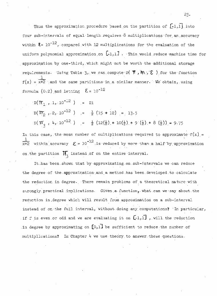
Thus the approximation procedure based...on. the p a r t i t i o n of j j - l . , l ~ J . i n t o
four s u b - i n t e r v a l s of e q u a l ; l e n g t h r e q u i r e s 8 m u l t i p l i c a t i o n s for, an.accuracy -1 P
wi t h i n E= 10 ,.compared ..with. 12 m u l t i p l i c a t i o n s for.'the e v a l u a t i o n of the
uniform polynomial.approximation ,on . - This.would reduce machine time f o r
approximation by one-third,, which might not be worth t h e • a d d i t i o n a l storage requirements. Using Table -3, :we can. compute p( T , \y\ ,~Z ) . f o r the f u n c t i o n
1
f ( x ) = x+2 and the same p a r t i t i o n s - i n ; a s i m i l a r , manner. • We" obtain,. u s i n g
formula (0.2) .and ..letting £ = 1 0 ~ 1 2
-D(1T1 , .1,. 1 0 " 1 2 ) .= 21
D(TT2 , ) 2 , 1 0 - 1 2 ) ,.= \ (15.+ 12) .,= , 13.5
D(TT3 , . U , 1 0 - 1 2 ) ,= \ (12(£.).+ 1 0 ( | ) . + 9 (|),+ 8 (±)),=9»75
In t h i s c a s e , : t h e mean number of m u l t i p l i c a t i o n s r e q u i r e d to approximate f ( x ) , = —— -12
x+2 w i t h i n accuracy £.= 10 ..is reduced by more than a h a l f by approximation
on the p a r t i t i o n Tf^ . i n s t e a d ..of on the e n t i r e - i n t e r v a l .
It,.has been ..shown t h a t by-approximating on. s u b - i n t e r v a l s we can:reduce
the degree of the : approximation ..and a method has been. developed to c a l c u l a t e
the r e d u c t i o n . i n degree.. There remain problems - of a t h e o r e t i c a l nature w i t h
strongly, p r a c t i c a l i m p l i c a t i o n s . Given ,a function,., what can we - say about, the
r e d u c t i o n in.degree which w i l l r e s u l t from approximation on a s u b - i n t e r v a l
, i n s t e a d of on the f u l l , i n t e r v a l , without doing any, computations? 'In p a r t i c u l a r ,
i f f i s even or odd and .we are e v a l u a t i n g i t on C-l>l-I , . w i l l . t h e r e d u c t i o n
i n degree by approximating on |~0,ll be s u f f i c i e n t to reduce the number of
m u l t i p l i c a t i o n s ? 'In: Chapter k we use theory.to answer, these questions.

CHAPTER 4 2 4 *
THEORETICAL CONSIDERATIONS ON SHORTENING THE INTERVAL OF APPROXIMATION
In the c l a s s o f a l l polynomials of degree n there e x i s t s a unique polynomial
approximation, c a l l e d the best uniform polynomial approximation of degree n,
which minimizes AP. We denote t h i s minimal value of &P by E n or E n ^ a ^ i 3 .
For a given continuous f u n c t i o n f, • a,b i s a. f u n c t i o n of n,a,. and b. We
would l i k e t o estimate E ^ g ^ without extensive • computation. and we consider
e s t i m a t i o n of E n ^ a ^ by use-of e a s i l y determined upper bounds.
Jackson.has obtained s e v e r a l r e s u l t s £6, pp.13-18"] g i v i n g bounds f o r En,a,b ^ w o °^ 'these f o l l o w .
Theorem 1 I f f s a t i s f i e s the c o n d i t i o n |f ( x ^ ) - f ( x 2 ) | -6 >\ |..x-]_-x2 |
f o r a l l x x and Xg i n La^bJ , then E ^ ^ t , 4 L(b.-a)X
Theorem 2 I f f has a p t h d e r i v a t i v e f ^ ^ ( x ) s a t i s f y i n g
| f ( j f ) ( x 1 ) - f ( : P > ) ( x 2 ) I ^ X I. X - L - X 2 I f o r a l l x± and x 2 i n [a,b] ,
.then f o r a l l n a t u r a l numbers n, n ik..p,
E ^ ( P :+ I f L P + 1 ( b - a ) ^ + 1 \
n n P + 1 p!
L i s - a u n i v e r s a l constant and may be taken as L = \ i n these theorems.
Jackson gives other r e s u l t s . i n terms of the modulus of c o n t i n u i t y .
A bound f o r ^ ^ can a l s o be d e r i v e d from the remainder formula f o r
Lagrange i n t e r p o l a t i o n . The k t h Chebyshev polynomial on fa,b] i s defined to
be T k a b = c o s arc cos (^f— (2x-a-b))) .(4.1)
.= T k (_i_ (2x-a-b)) . (4.2) ' b-a
Let L ^ a ^ be the Lagrange i n t e r p o l a t i o n polynomial of degree n f i t t e d to f
at the zeros of the n+1 s t Chebyshev polynomial on [a,b~] . I t can e a s i l y be
shown th a t L ^ a ^ has-a t r u n c a t i o n e r r o r bound
^ ^ a ; t = S1±P _lf(x) - I^a, b< (x) ) (4.3) x 6 La,b J
25-
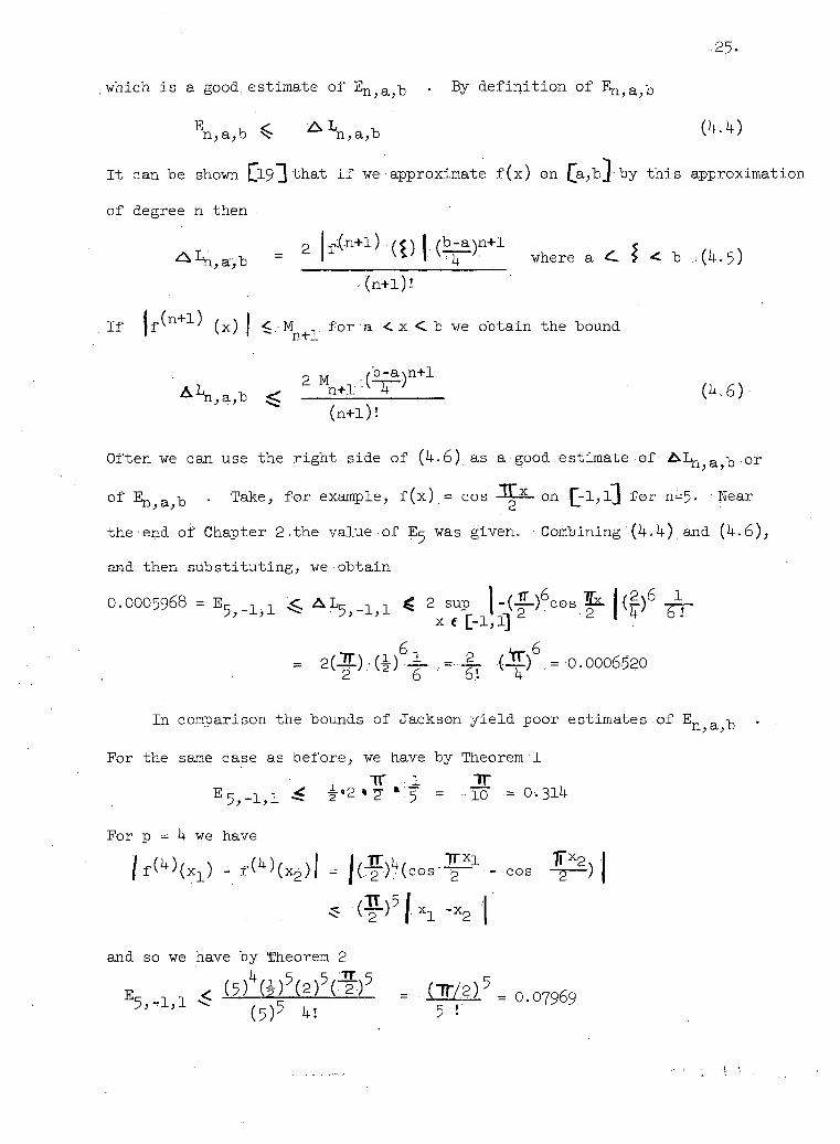
which i s a good, estimate of E N ^ A J D • By d e f i n i t i o n of E ^ g ^
En,a,b ^ A L n , a , b
I t can be shown 0-9"] that i f we • approximate f ( x ) on (ja,bT] by this-approximati
of degree n then i o n
^ , f f , b = 2 f,(.n+l) .(^) |,(b-a)n+l & ^ f < b ; ( k > 5 )
(n+1)!
I f jf(n+1) (x) j <-M for-a < x < b we obtain the bound
2 l , : ^ ) n + 1 ^ n + l ! V ^ ( ,„6) • (n+1)!
Often we can use the righ t side of (4.6), as a good estimate of AIfr,a,b o r
of En^a^-b . Take, for example, f ( x ) = cos on Q - l , l ] f o r n=5- Near
the end of Chapter 2 .the value of was given. Combining (4.4),and (4 .6) ,
and then substituting, we obtain
0.0005968 = ^ A L 5 ) . 1 ; 1 * - 2 sup | - ( X ) 6 C O B | L I (2)6 l ^ x ( C-l, l j
In comparison the bounds.of Jackson y i e l d poor estimates of E n a
For the same case as before, we have by Theorem'1
TT • 1 "TT E 5 , - l , l ^ i ' 2 « 2 * : 5 = •'•"io •= 0.314
For p = 4 we have
- fC*)(x2)| - |cf)f(=o.-^-.cM ) | ^ ( ")5 f x 1 -x 2 j
and so we have by Theorem 2
E 5 ^^Lihk^Ml - a m 5 = 0.07969
26.
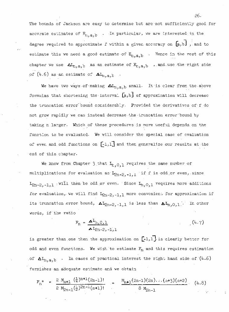
The bounds of Jackson are easy to determine but are not s u f f i c i e n t l y good f o r
accurate estimates of IL „ y. . In p a r t i c u l a r , we are i n t e r e s t e d i n the
degree required, to approximate f w i t h i n a given accuracy on (a,b"l ,. and t o
estimate t h i s we need a good estimate of E n a . Hence i n the r e s t of t h i s
chapter we use A I ^ a ft . as • an estimate of a ,. and. use the r i g h t side
.of (4.6) as an estimate of A I ^ •
We have two ways of making A I ^ a -0 small. I t - i s - c l e a r from the - above
formulas t h a t shortening t h e • i n t e r v a l [a,b3 of approximation w i l l decrease
the t r u n c a t i o n e r r o r bound con s i d e r a b l y . Provided the d e r i v a t i v e s of f do
not grow r a p i d l y we can i n s t e a d decrease the t r u n c a t i o n e r r o r bound by
t a k i n g n , l a r g e r . Which of these procedures i s more u s e f u l depends, on the
f u n c t i o n to be evaluated. We w i l l , c o nsider the s p e c i a l . c a s e ,of e v a l u a t i o n
of even and odd.functions on Q-l,l] and then g e n e r a l i z e our r e s u l t s at the
end o f t h i s chapter.
We know from Chapter 3 .that LQ . 0 ]_ r e q u i r e s the same • number of
m u l t i p l i c a t i o n s f o r e v a l u a t i o n a s l < 2 n _ 2 - 1 1 ^ ^ is-odd.or even, . since
I j 2 n - 2 _2_ j_ : w i l l then.be odd or even. Since L ^ Q ^ r e q u i r e s more a d d i t i o n s
f o r e v a l u a t i o n , we w i l l f i n d I < 2 n _ 2 , - . 1 , 1 more convenient f o r approximation i f
i t s t r u n c a t i o n .error bound, - ^ I j 2 n - 2 , - . 1 , 1 i s l e s s than A l ^ o,l'"* l ' n other
words, i f ' t h e r a t i o
F n = A L n , 0 , l (4.7)
A L 2 n - 2 , - l ' , I
i s g r e a t e r than.one then the approximation on Q-l,l"3 i s c l e a r l y b e t t e r f o r
odd and even f u n c t i o n s . We wish t o estimate F n and t h i s r e q u i r e s e s t i m a t i o n
.of A l h a ^ In cases of p r a c t i c a l i n t e r e s t the r i g h t hand side of (4.6)
f u r n i s h e s an.adequate estimate and.we o b t a i n
V = 2 V i (i) n + 1( g"-l) ! = M n + 1 ( 2 n - l ) ( 2 n ) . . . ( n H - 3 ) ( n + 2 ) ( ^ g )
2 M 2 n _ i ( i ) 2 n - 1 ( n + l ) ! 8 -
27-
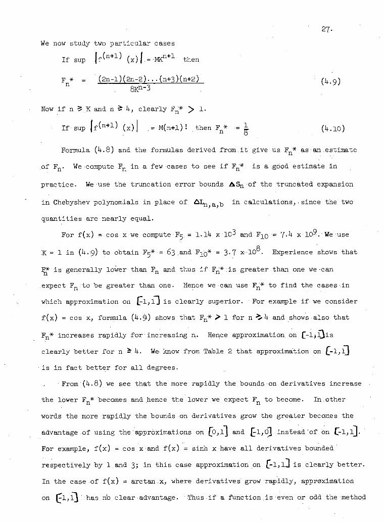
We now study two p a r t i c u l a r cases
I f sup |f<n+l) ( x ) | = MK n + 1 then
F-* = (2n-l)(2n-2) . . • (n+3)(n+2) ( k - 9 ) n 8 K n " 3
Now i f n 5 X and n £ 4 , c l e a r l y F N * > 1.
I f sup | f ( n + 1 ) ( x ) | ,=M(n+l)! then F n * .•= 1 (4.10)
Formula (4.8) and the formulas d e r i v e d f r o m . i t give us F n * as an e s t i m a t e
of F n. We compute F n i n a few-cases t o s e e . i f F n * i s a good e s t i m a t e • i n
p r a c t i c e . We use the t r u n c a t i o n e r r o r bounds A S n of the tru n c a t e d expansion
i n Chebyshev polynomials i n pl a c e of ^ I ^ a ^ i n c a l c u l a t i o n s , : s i n c e the two
q u a n t i t i e s are n e a r l y equal.
For f ( x ) = cos x we compute F^ = 1.14 x 10^ and F^Q = 7>4 x lO^.Weuse o
X = 1 i n (4.9) to o b t a i n F5* = 63 .and F 1 0 * - 3.7 x-10° . Experience shows t h a t
F* i s g e n e r a l l y lower than'F n and thus i f F n * . ; i s greater than one we-can
expect F n . t o be grea t e r than one. Hence we-can use F n * to f i n d the c a s e s - i n
which approximation on f l , l ] i s c l e a r l y s u p e r i o r . For example i f we consider
f ( x ) = cos x, formula (4.^) shows t h a t F n * > l f o r n ^ and shows-also t h a t
F n * increases r a p i d l y f o r i n c r e a s i n g n. Hence approximation, on £-l>l^is
c l e a r l y b e t t e r f o r n - . 4 . We- know from Table 2 t h a t approximation on £-l,l]
• i s i n f a c t b e t t e r f o r a l l degrees.
From (4.8) we see tha t the more r a p i d l y the bounds on d e r i v a t i v e s increase
the lower F n * becomes and hence-the lower we expect F n to become. In.other
words the more r a p i d l y the bounds on d e r i v a t i v e s grow the gre a t e r becomes the
advantage of u s i n g the approximations on £p,l"] and £-1,(5] .instead'of on £l,l~|.
For example, f ( x ) = cos x and f ( x ) = si n h x have a l l d e r i v a t i v e s bounded
r e s p e c t i v e l y by 1 and 3; i n t h i s case approximation on £-1,1-3 i s c l e a r l y b e t t e r .
In the case of f ( x ) = a r c t a n x , where d e r i v a t i v e s grow r a p i d l y , approximation
on (^l,l3:.has ho clear-advantage. Thus i f a f u n c t i o n i s even or odd the method
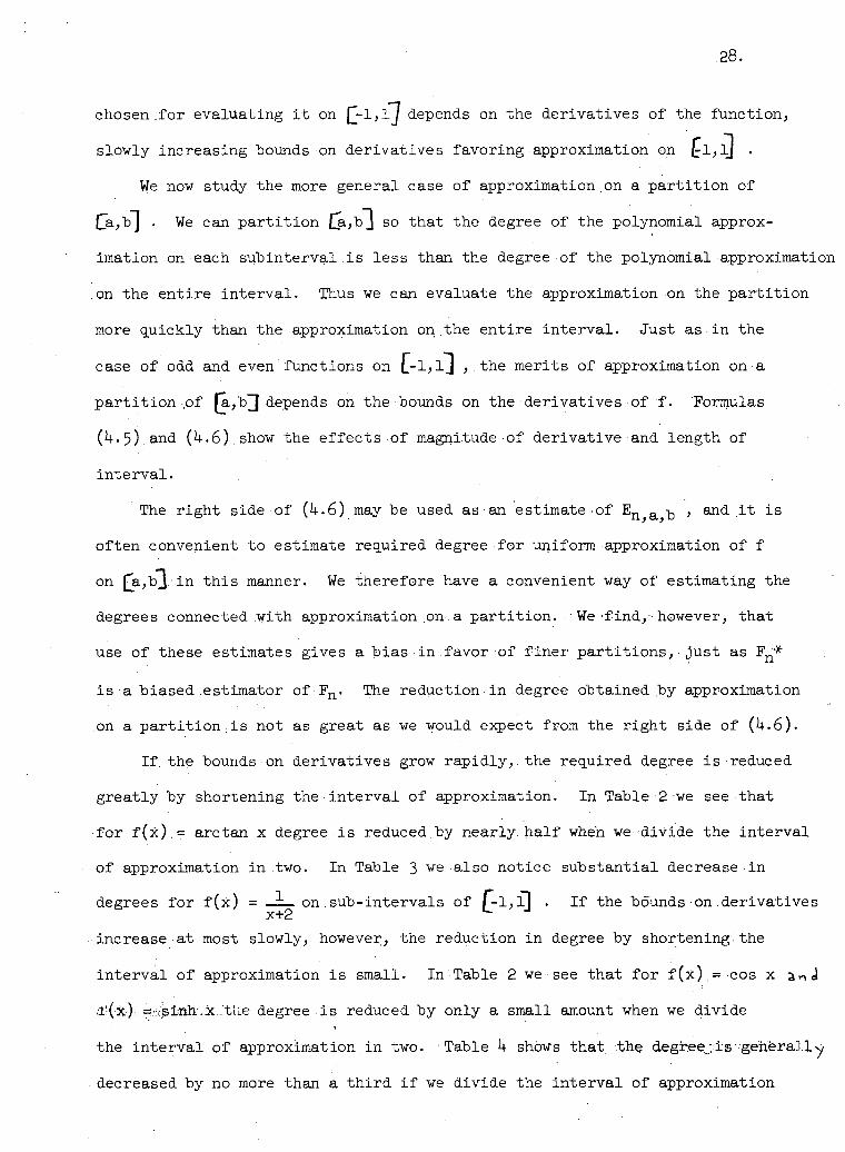
.28.
chosen ..for e v a l u a t i n g i t on Q-l,lJ depends on the d e r i v a t i v e s of the f u n c t i o n ,
s l o w l y i n c r e a s i n g hounds on d e r i v a t i v e s f a v o r i n g approximation on £l,l] •
We now study the more general case of approximation.on a p a r t i t i o n of
Ca,b~] . We can p a r t i t i o n [LajT l so t h a t the degree of the polynomial approx
imation on each s u b i n t e r v a l i s l e s s than the degree of the polynomial approximation
on the e n t i r e i n t e r v a l . Thus we can evaluate the approximation on the p a r t i t i o n
more q u i c k l y than the approximation on the e n t i r e i n t e r v a l . J u s t as i n the
case of odd and even f u n c t i o n s on £-l,l] , the m e r i t s of approximation on ;a
p a r t i t i o n ,of (a,b^J depends on the bounds on the d e r i v a t i v e s of f. Formulas
( 4 . 5 ) .and (4.6).show the e f f e c t s of magnitude • of d e r i v a t i v e and l e n g t h of
i n t e r v a l .
The r i g h t side of (4-6) may be used as an estimate of E n ^ , and i t i s
o f t e n convenient t o estimate r e q u i r e d degree f o r uniform approximation of f
on fja,b"3 i n t h i s manner. We t h e r e f o r e have a convenient way of e s t i m a t i n g the
degrees connected w i t h approximation on.a p a r t i t i o n . . We f i n d , - however, t h a t
use of these estimates gives a b i a s i n f a v o r of f i n e r p a r t i t i o n s , j u s t as F n *
i s a b i a s e d estimator of F n. The r e d u c t i o n . i n degree obtained by.approximation
on a p a r t i t i o n ; i s not as great as we would expect from the r i g h t side of (4 .6) .
If. the bounds on d e r i v a t i v e s grow r a p i d l y , . t h e . r e q u i r e d degree i s reduced
g r e a t l y by shortening the i n t e r v a l of approximation. In Table 2 we see t h a t
•for f ( x ) . = a r c t a n x degree i s reduced by n e a r l y h a l f when we-divide the i n t e r v a l
of approximation i n two. In Table 3 we a l s o n o t i c e s u b s t a n t i a l decrease i n
degrees f o r f ( x ) = — i — o n . s u b - i n t e r v a l s of | - l , l ] . I f the bounds o n . d e r i v a t i v e s x+2
increase at most slowly, however, the r e d u c t i o n i n degree by s h o r t e n i n g i t h e
i n t e r v a l o f approximation i s small. In Table 2 we see t h a t f o r f ( x ) = cos x a ^ J
.l-(-x).;. 5.:,isinh:.x...'tue degree i s reduced by only a small amount when we d i v i d e
the i n t e r v a l o f approximation i n two. Table 4 shows t h a t the degree i s g e n e r a l l y
decreased by no more than a t h i r d i f we d i v i d e the i n t e r v a l of approximation
i n t o f o u r p a r t s f o r f (x) = e x. For the general case of approximation of a
continuous f u n c t i o n on.a p a r t i t i o n of £a b3 , we conclude t h a t a f i n e r
p a r t i t i o n of [a.,h\ D ecomes more advantageous the more r a p i d l y the bounds on
the d e r i v a t i v e s of f increase. I f the bounds on the d e r i v a t i v e s - o f f increase
s l o w l y , the use of approximation ; on, a p a r t i t i o n i s not of great b e n e f i t .
3©'.
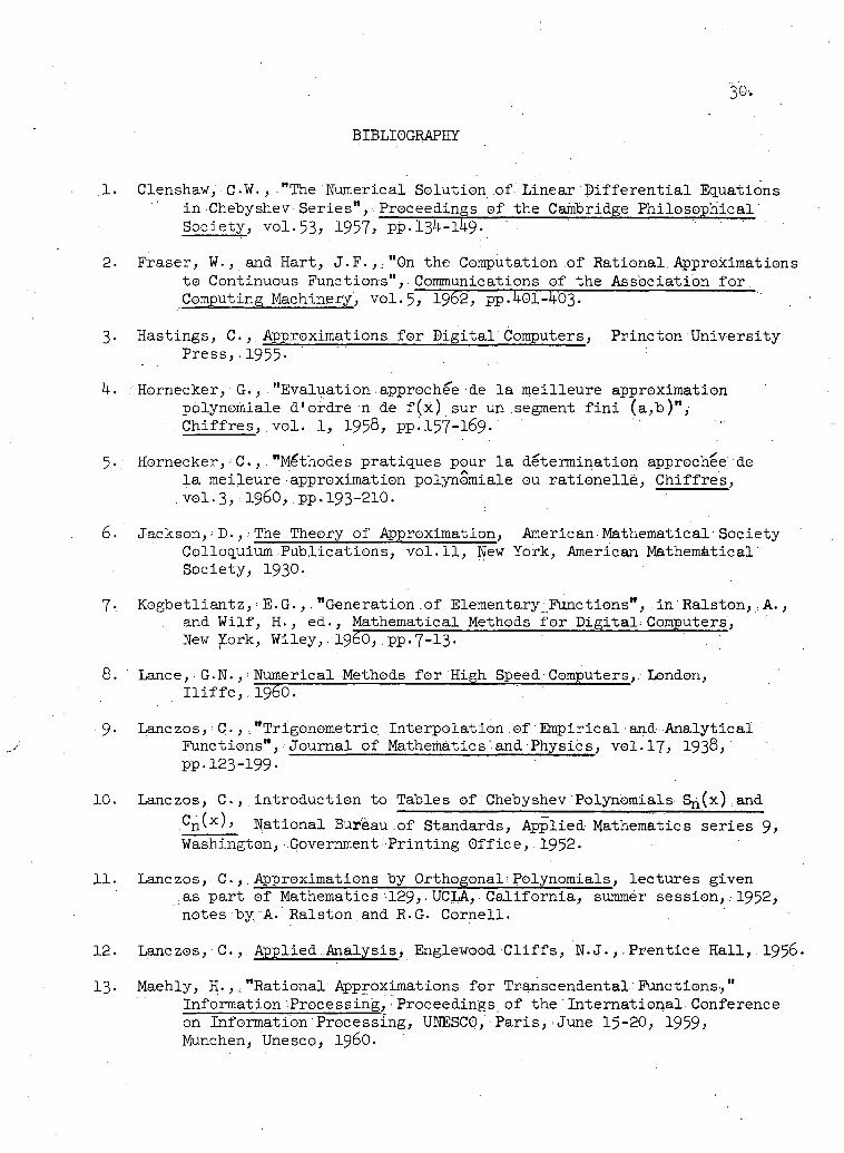
BIBLIOGRAPHY
.1. Clenshaw, C-W., "The Numerical.Solution of- L i n e a r D i f f e r e n t i a l Equations i n Chebyshev S e r i e s " , • Proceedings of the Cambridge P h i l o s o p h i c a l S o c i e t y , v o l . 5 3 , 1957, pp.13 k - l49. ~
2. F r a s e r , W., and Hart, J.F.,,"On the Computation of R a t i o n a l . Approximations t o Continuous Functions",• Communications of the A s s o c i a t i o n f o r Computing Machinery, v o l . 5 , ' 1962, pp.401-403- ""
3. Hastings, C.,. Approximations f o r D i g i t a l ' Computers, P r i n c t o n U n i v e r s i t y Press,.1955. ' ' ' '
4. Hornecker, G.,."Evaluation approchee de l a m e i l l e u r e approximation polynomiale d'ordre n de f ( x ) sur un .segment f i n i ( a,b)",
. C h i f f r e s , v o l . . 1, 1958, pp.157-169.'
5-; Hornecker, ;C.,."Mlthodes p r a t i q u e s pour l a determination approchee de l a meileure approximation polynomiale ou r a t i o n e l l e , C h i f f r e s , v o l . 3 , i960,.pp.193-210.
6. Jackson, ; D . T h e Theory of Approximation, American Mathematical-Society C o l l o q u i u m - P u b l i c a t i o n s , v o l . 1 1 , New York,. American Mathematical S o c i e t y , 1930.
7- K o g b e t l i a n t z , •• E. G.,, "Generation of Elementary^Functions", i n R a l s t o n , ; A., and W i l f , H., ed., Mathematical Methods f o r D i g i t a l ^ Computers, New York, Wiley,. i960, pp .7-13. ~ ~
8. Lance, G.N., - Numerical Methods f o r High Speed-Computers, London, I l i f f c , i960. ' " ' ~
9- Lanczos, : C - " T r i g o n o m e t r i c I n t e r p o l a t i o n .of E m p i r i c a l ; a n d - A n a l y t i c a l F u n c t i o n s " , - J o u r n a l of Mathematics'and P h y s i c s , vol. 1 7 , 1938,' pp.123-199-
10. Lanczos, C., i n t r o d u c t i o n to Tables of Chebyshev Polynomials S^Cx)<and . n N a t i o n a l Bureau.of Standards, A p p l i e d Mathematics s e r i e s 9, Washington, .Government-Printing O f f i c e , , 1952.
11. Lanczos, • C.,. Approximations by Orthogonal; Polynomials, l e c t u r e s given .as p a r t of Mathematics 129, - UCLA, C a l i f o r n i a , summer session,.1952, notes by A. R a l s t o n and R.G. C o r n e l l .
12. L a n c z o s , C , A p p l i e d A n a l y s i s , Englewood C l i f f s, N.J.,. P r e n t i c e H a l l , . 1956-
13. Maehly, H . , : " R a t i o n a l : Approximations f o r Transcendental Functions," Information Processing,<Proceedings of the I n t e r n a t i o n a l . Conference on Information P r o c e s s i n g , UNESCO,•Paris,-June 15-20, 1959, Munchen, Unesco, i960.
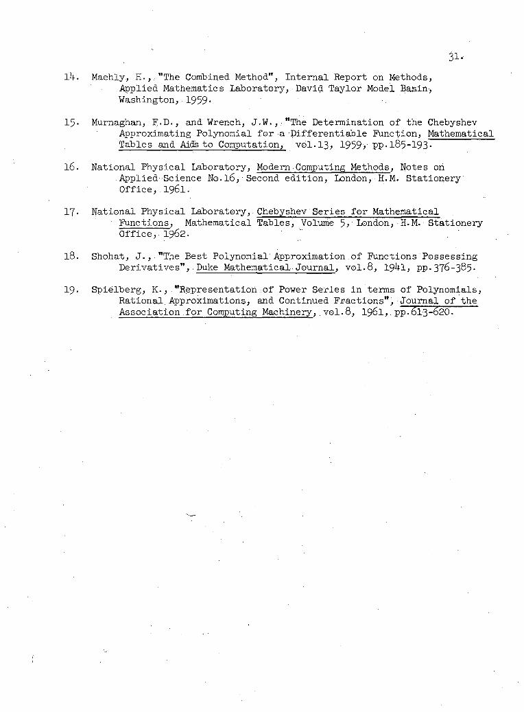
31.
lk. Maehly, H.,,"The Combined Method",. I n t e r n a l Report on Methods, , A p p l i e d Mathematics Laboratory, David T a y l o r Model Ba s i n , Washington,. 1959-
15- Murnaghan, F.D., and Wrench, J.W.,,"The Determination of the Chebyshev Approximating Polynomial f o r a D i f f e r e n t i a b l e Function, Mathematical Tables and Aids t o Computation, v o l . 1 3 , 1959> PP-185-193-
16. N a t i o n a l P h y s i c a l Laboratory, Modern•Computing Methods, Notes on A p p l i e d Science No. 16, •• Second e d i t i o n , London, H.M. St a t i o n e r y " Office,. 1 9 6 1 .
17. N a t i o n a l P h y s i c a l Laboratory, Chebyshev S e r i e s f o r Mathematical • Functions, Mathematical Tables, Volume 5> London,•H.M. • S t a t i o n e r y
O f f i c e , 1962.
18. Shohat, J . , "The Best Polynomial.Approximation of Functions Possessing Derivatives",.Duke Mathematical J o u r n a l , v o l . 8 , 19kl, pp.376-385-
19. S p i e l b e r g , K.,."Representation of Power S e r i e s i n terms of Polynomials, R a t i o n a l Approximations, and Continued F r a c t i o n s " , J o u r n a l o f the A s s o c i a t i o n f o r Computing Machinery, v o l . 8 , 1961, pp .6 l3-620.
Recommended


![Interpolation & Polynomial Approximation [0.125in]3.625in0.02in …mamu/courses/231/Slides/CH03_3A.pdf · 2012-08-02 · Interpolation & Polynomial Approximation Divided Differences:](https://img.pdfslide.us/doc/110x75/5f5234d5ff877a36963dc704/interpolation-polynomial-approximation-0125in3625in002in-mamucourses231slidesch033apdf.jpg)
![Interpolation & Polynomial Approximation [0.125in]3.625in0 ...mamu/courses/231/Slides/...A good interpolation polynomial needs to provide a relatively accurate approximation over an](https://img.pdfslide.us/doc/110x75/6105aa5678fd697b956f2428/interpolation-polynomial-approximation-0125in3625in0-mamucourses231slides.jpg)


![Interpolation & Polynomial Approximation [0.125in]3.625in0](https://img.pdfslide.us/doc/110x75/61caec2c5334682d856ac40e/interpolation-amp-polynomial-approximation-0125in3625in0-.jpg)