UNDERGRADUATE RESEARCH THESIS
A METHODOLOGY FOR THE ROBUST PROCEDURE
DEVELOPMENT OF FILLET WELDS
Submitted to:
The Ohio State University Knowledge Bank
Submitted By:
Paul Boulware
Senior, Welding Engineering Program
5720 Aspendale Dr.
Columbus, Ohio 43235
May 19, 2006
Executive Summary
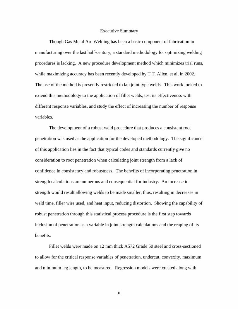
Though Gas Metal Arc Welding has been a basic component of fabrication in
manufacturing over the last half-century, a standard methodology for optimizing welding
procedures is lacking. A new procedure development method which minimizes trial runs,
while maximizing accuracy has been recently developed by T.T. Allen, et al, in 2002.
The use of the method is presently restricted to lap joint type welds. This work looked to
extend this methodology to the application of fillet welds, test its effectiveness with
different response variables, and study the effect of increasing the number of response
variables.
The development of a robust weld procedure that produces a consistent root
penetration was used as the application for the developed methodology. The significance
of this application lies in the fact that typical codes and standards currently give no
consideration to root penetration when calculating joint strength from a lack of
confidence in consistency and robustness. The benefits of incorporating penetration in
strength calculations are numerous and consequential for industry. An increase in
strength would result allowing welds to be made smaller, thus, resulting in decreases in
weld time, filler wire used, and heat input, reducing distortion. Showing the capability of
robust penetration through this statistical process procedure is the first step towards
inclusion of penetration as a variable in joint strength calculations and the reaping of its
benefits.
Fillet welds were made on 12 mm thick A572 Grade 50 steel and cross-sectioned
to allow for the critical response variables of penetration, undercut, convexity, maximum
and minimum leg length, to be measured. Regression models were created along with
ii
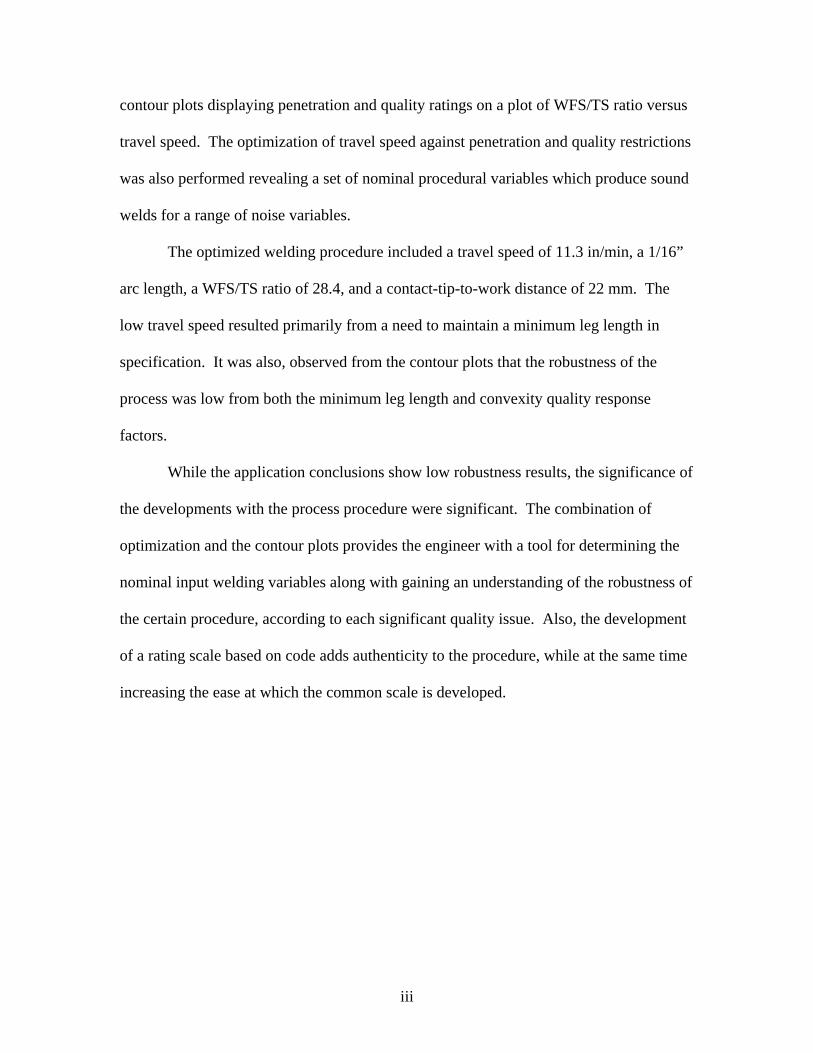
contour plots displaying penetration and quality ratings on a plot of WFS/TS ratio versus
travel speed. The optimization of travel speed against penetration and quality restrictions
was also performed revealing a set of nominal procedural variables which produce sound
welds for a range of noise variables.
The optimized welding procedure included a travel speed of 11.3 in/min, a 1/16”
arc length, a WFS/TS ratio of 28.4, and a contact-tip-to-work distance of 22 mm. The
low travel speed resulted primarily from a need to maintain a minimum leg length in
specification. It was also, observed from the contour plots that the robustness of the
process was low from both the minimum leg length and convexity quality response
factors.
While the application conclusions show low robustness results, the significance of
the developments with the process procedure were significant. The combination of
optimization and the contour plots provides the engineer with a tool for determining the
nominal input welding variables along with gaining an understanding of the robustness of
the certain procedure, according to each significant quality issue. Also, the development
of a rating scale based on code adds authenticity to the procedure, while at the same time
increasing the ease at which the common scale is developed.
iii
Table of Contents
Executive Summary………………………………………………………………... ii
1.0 Introduction………………………………………………………………… 1
2.0 Background………………………………………………………………… 2
3.0 Objectives..………………………………………………………………… 5
4.0 Experimental Procedure……………………………………………………. 5
4.1 Selection of variables: Factors and Responses……………………. 6
4.1.1 Factors: Input Variables…………………………………… 6
4.1.2 Factors: Noise Variables…………………………………... 7
4.1.3 Response Variables………………………………………… 8
4.2 Preliminary Testing………………………………………………… 8
4.3 Experimental Design……………………………………………….. 13
4.4 Experimental Welding………………………………………………16
4.5 Response Measuring Procedure……………………………………. 18
5.0 Results and Discussion…………………………………………………….. 20
5.1 Regression………………………………………………………….. 20
5.1.1 Rating Scale………………………………………………... 20
5.1.2 Regression Models…………………………………………. 23
5.2 Contour Plots………………………………………………………. 25
5.3 Optimization……………………………………………………….. 29
5.4 Confirmation Runs…………………………………………………. 31
6.0 Conclusion…………………………………………………………………. 32
7.0 Future Work………………………………………………………………... 32
iv

8.0 Acknowledgements…………………………………………………………33
9.0 References…………………………………………………………………..35
v
1.0 INTRODUCTION
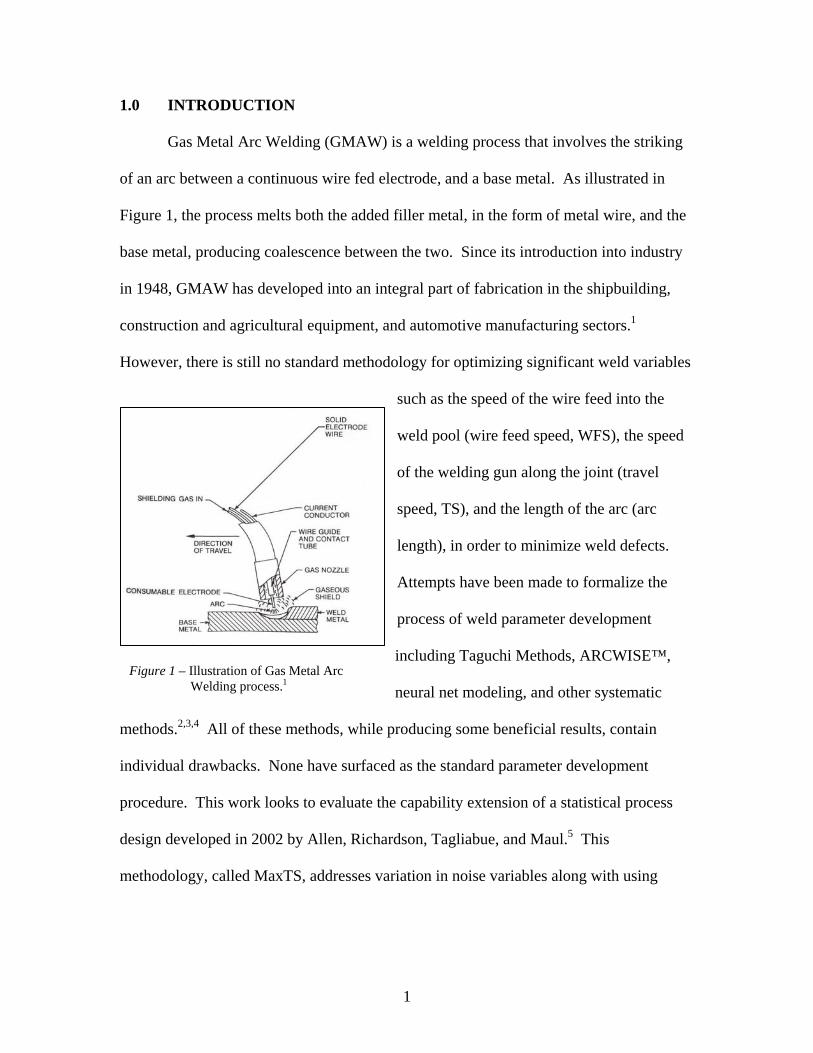
Gas Metal Arc Welding (GMAW) is a welding process that involves the striking
of an arc between a continuous wire fed electrode, and a base metal. As illustrated in
Figure 1, the process melts both the added filler metal, in the form of metal wire, and the
base metal, producing coalescence between the two. Since its introduction into industry
in 1948, GMAW has developed into an integral part of fabrication in the shipbuilding,
construction and agricultural equipment, and automotive manufacturing sectors.1
However, there is still no standard methodology for optimizing significant weld variables
such as the speed of the wire feed into the
weld pool (wire feed speed, WFS), the speed
of the welding gun along the joint (travel
speed, TS), and the length of the arc (arc
length), in order to minimize weld defects.
Attempts have been made to formalize the
process of weld parameter development
including Taguchi Methods, ARCWISE™,
neural net modeling, and other systematic
methods.2,3,4 All of these methods, while producing some beneficial results, contain
individual drawbacks. None have surfaced as the standard parameter development
procedure. This work looks to evaluate the capability extension of a statistical process
design developed in 2002 by Allen, Richardson, Tagliabue, and Maul.5 This
methodology, called MaxTS, addresses variation in noise variables along with using
Figure 1 – Illustration of Gas Metal Arc Welding process.1
1
unique welding input variables to increase accuracy and help better focus the region of
interest with the experimentation, respectively.
This study looks to increase the strength of this procedural design process by
evaluating the inclusion of different response variables along with studying the effect of
doubling the number of response variables. Also, included for the developments found
through this work is a move away from the user defined rating system for response
variables. Greater detail concerning this statistical process design and the development
proposed with this work is provided in the following section.
To investigate these proposed improvements the application of a robustness
evaluation for an industrial GMAW procedure was chosen. This allowed for the new
response variables of joint penetration, undercut, concavity, and weld aspect ratio to be
incorporated into the experimental design.
2.0 BACKGROUND
Many methodologies and procedures have been developed and utilized for
welding procedural development including the use of Taguchi methods, neural net
models, and simple trial and error heuristic methods. While all of these methods have
their advantages, the statistical process design procedure included with MaxTS manifests
benefits over each. The method avoids the inaccuracy issues of Taguchi Methods, the
special software and training of neural net models, and limits the number of necessary
trial runs characteristic of heuristic methods.6 A difference is also seen in comparison to
the ARCWISE™ procedure which categorizes welds only into an acceptable or
unacceptable range.3 The new methodology incorporates a more systematic rating scale,
resulting in a highly informative tool for determining, not only a clear-cut conclusion of
2
the acceptability of the procedure, but also information on how close the procedure is to
such a boundary.
The methodology developed by Allen et al5, shows significant improvements in
welding procedural development through incorporation of noise factor variance and also
through unique choices in the selection of independent factors. Permitting variance of the
noise factors within the experimental design and analysis makes the procedure
comparable to Taguchi signal-to-noise ratios.2 The advantage, however, is found within
this method’s ability to allow for the use of classically designed experiments and
optimization, in conjunction with noise factor variance. Taguchi methods prevent the
utilization of standard designed experiments and optimization.
The second advantage found with this statistical process design is the use of arc
length and wire feed speed to travel speed (WFS/TS) ratio in place of voltage and wire
feed speed, respectively. Using arc length rather than voltage avoids the inclusion of a
significant number of poor welds in the experimental array, while incorporation of
WFS/TS ratio allows control of the weld size to be maintained.5
Classically designed experiments have the characteristic of running
experimentation at the limits of the selected factor ranges. When using voltage and wire
feed speed as independent factors, settings composed of high voltage and low wire feed
speed, and low voltage with high wire feed speed result. Both of these cases result in
extremely poor welds with immeasurable characteristics. This is due to the fact that the
first case mentioned results in arc lengths at the extreme high limit while the second
condition produces arc lengths at the extreme low limit. Both cases produce
unacceptable welds. Simply incorporating arc length in the place of voltage in the
3
experimental design eliminates this problem and helps improve the accuracy of the
calculated regression models.
Using the WFS/TS ratio as an independent variable ensures that each
experimental weld is of a reasonable size. This incorporates the important factor of wire
feed speed in the procedure, but does it in a controlled manner. Again, this leads to
concentrating the experimental welds in the region of space desired by the user and also
increases the accuracy of the experiment.5
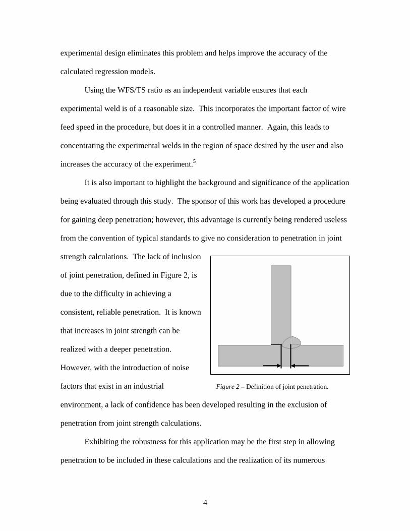
It is also important to highlight the background and significance of the application
being evaluated through this study. The sponsor of this work has developed a procedure
for gaining deep penetration; however, this advantage is currently being rendered useless
from the convention of typical standards to give no consideration to penetration in joint
strength calculations. The lack of inclusion
of joint penetration, defined in Figure 2, is
due to the difficulty in achieving a
consistent, reliable penetration. It is known
that increases in joint strength can be
realized with a deeper penetration.
However, with the introduction of noise
factors that exist in an industrial
environment, a lack of confidence has been developed resulting in the exclusion of
penetration from joint strength calculations.
Figure 2 – Definition of joint penetration.
Exhibiting the robustness for this application may be the first step in allowing
penetration to be included in these calculations and the realization of its numerous
4
benefits. Smaller weld sizes would be possible, allowing for reduced weld times and
filler metal usage. Also, decreases in the heat into the weld would reduce distortion.
This would result in substantial savings in mass production industries. Manifestation of a
robust process for deep penetration in GMAW is a main step in allowing for the inclusion
of penetration in joint strength calculations, and thus a major step towards achieving its
monetary benefits.
3.0 OBJECTIVES
The main objective of this work is to further strengthen the statistical process
procedure called MaxTS developed in 2002 by Allen et al5, through extending its range
of applications and variables. More specific goals of this study are outlined in the
following:
• Demonstrate reliability and robustness in producing welds with a given
penetration, allowing the dimension of joint penetration to be considered for the
joint strength relationships found in standards and codes.
• Produce empirical models for prediction of joint penetration and the pertinent
quality issues for the application of deep penetration GMAW of fillet welds.
• Provide a set of welding parameters to maximize travel speed while holding a
level of satisfactory penetration along with quality levels above the limits defined
by AWS D14.3.
4.0 EXPERIMENTAL PROCEDURE
The experimental approach was established to test the adaptiveness of the
statistical process design procedure, MaxTS, to a new weld and joint type, along with
distinctively different response variables. The total process is detailed in the following
sections.
5
4.1 Selection of Variables: Factors and Responses
4.1.1 Factors: Input Variables
It has been observed that the use of the standard welding input variables of travel
speed (TS), wire feed speed (WFS), arc voltage (V), and contact-tip-to-work distance
(CTWD) can result in the production of an overabundant amount of defective welds
when using classically designed experiments. The reason for this resides with the
tendency of the designed experiments to test the limits of a poorly selected factor, which
results in extremely negative interactions with the other welding factors at certain levels.
For example, classically designed experiments test the limits of a cuboidal or
spherical region that is specified by the experiment designer. In a cuboidal designed
experiment using the standard welding input factors, welds would be made with very
high voltages and low wire feed speeds which lead to unacceptable lack of fusion issues.
Also, welds with low voltages and high wire feed speeds resulting in miniscule arc
lengths would be included in the experimental results. These welds exhibit buried arcs,
or simply no weld at all due to small arc lengths.
The typical method of combating this negative effect of the DOE is to limit the
ranges of the experimental factors. This technique is normally successful in reducing the
number of defective welds from the values discussed above, but it also results in the
narrowing of the factor ranges. With narrow ranges, empirical models carry less
significance because they are only applicable to a small window of input values.
This work along with the standard input variables of travel speed and CTWD
looked to use the factors of arc length, and WFS/TS ratio to replace voltage and current,
respectively. Using arc length as opposed to voltage allows the experiment to avoid
6
including heavily defective welds resulting from excessively high or low magnitudes of
arc length.
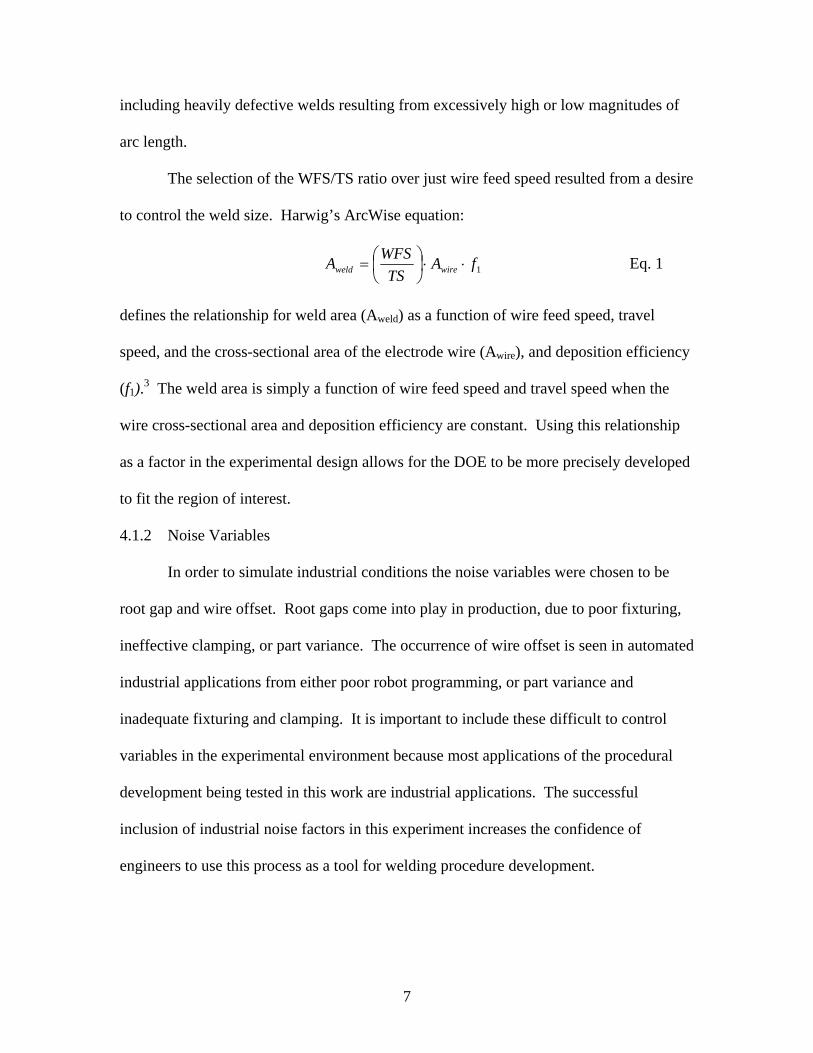
The selection of the WFS/TS ratio over just wire feed speed resulted from a desire
to control the weld size. Harwig’s ArcWise equation:
1fATS
WFSA wireweld ⋅⋅⎟⎠⎞
⎜⎝⎛= Eq. 1
defines the relationship for weld area (Aweld) as a function of wire feed speed, travel
speed, and the cross-sectional area of the electrode wire (Awire), and deposition efficiency
(f1).3 The weld area is simply a function of wire feed speed and travel speed when the
wire cross-sectional area and deposition efficiency are constant. Using this relationship
as a factor in the experimental design allows for the DOE to be more precisely developed
to fit the region of interest.
4.1.2 Noise Variables
In order to simulate industrial conditions the noise variables were chosen to be
root gap and wire offset. Root gaps come into play in production, due to poor fixturing,
ineffective clamping, or part variance. The occurrence of wire offset is seen in automated
industrial applications from either poor robot programming, or part variance and
inadequate fixturing and clamping. It is important to include these difficult to control
variables in the experimental environment because most applications of the procedural
development being tested in this work are industrial applications. The successful
inclusion of industrial noise factors in this experiment increases the confidence of
engineers to use this process as a tool for welding procedure development.
7
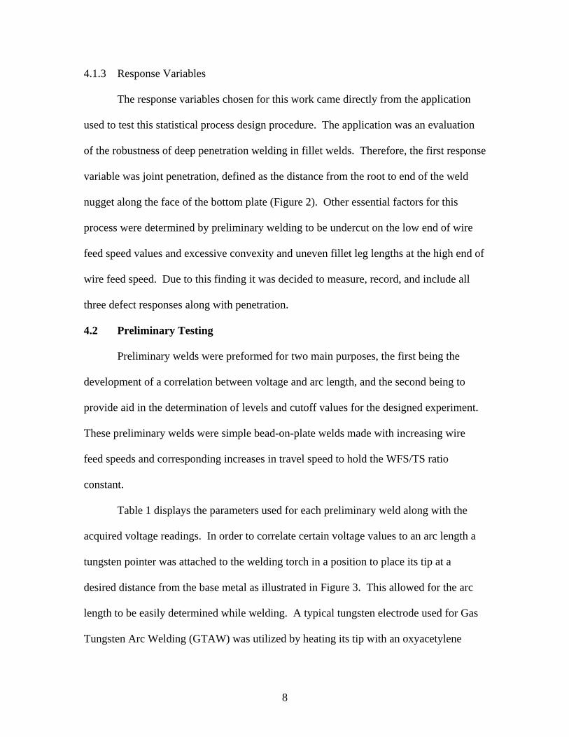
4.1.3 Response Variables
The response variables chosen for this work came directly from the application
used to test this statistical process design procedure. The application was an evaluation
of the robustness of deep penetration welding in fillet welds. Therefore, the first response
variable was joint penetration, defined as the distance from the root to end of the weld
nugget along the face of the bottom plate (Figure 2). Other essential factors for this
process were determined by preliminary welding to be undercut on the low end of wire
feed speed values and excessive convexity and uneven fillet leg lengths at the high end of
wire feed speed. Due to this finding it was decided to measure, record, and include all
three defect responses along with penetration.
4.2 Preliminary Testing
Preliminary welds were preformed for two main purposes, the first being the
development of a correlation between voltage and arc length, and the second being to
provide aid in the determination of levels and cutoff values for the designed experiment.
These preliminary welds were simple bead-on-plate welds made with increasing wire
feed speeds and corresponding increases in travel speed to hold the WFS/TS ratio
constant.
Table 1 displays the parameters used for each preliminary weld along with the
acquired voltage readings. In order to correlate certain voltage values to an arc length a
tungsten pointer was attached to the welding torch in a position to place its tip at a
desired distance from the base metal as illustrated in Figure 3. This allowed for the arc
length to be easily determined while welding. A typical tungsten electrode used for Gas
Tungsten Arc Welding (GTAW) was utilized by heating its tip with an oxyacetylene
8
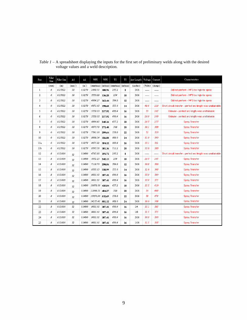
Table 1 – A spreadsheet displaying the inputs for the first set of preliminary welds along with the desired
voltage values and a weld description.
9
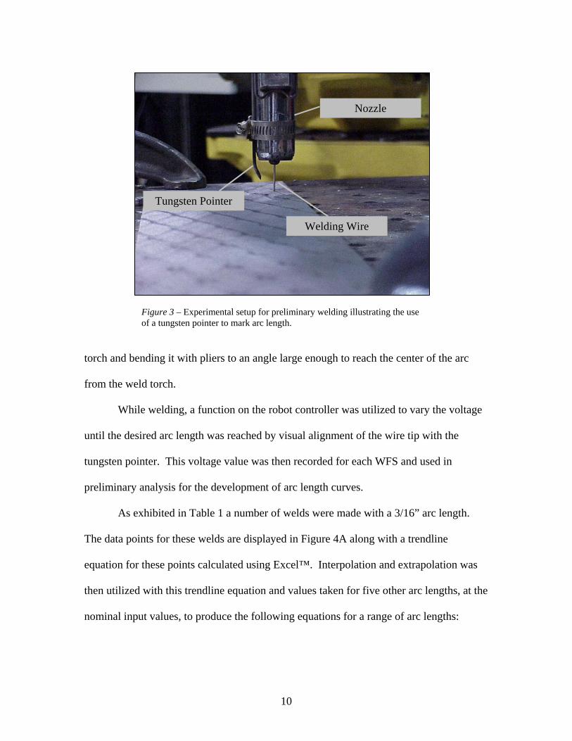
Tungsten Pointer
Welding Wire
Nozzle
Figure 3 – Experimental setup for preliminary welding illustrating the use of a tungsten pointer to mark arc length.
torch and bending it with pliers to an angle large enough to reach the center of the arc
from the weld torch.
While welding, a function on the robot controller was utilized to vary the voltage
until the desired arc length was reached by visual alignment of the wire tip with the
tungsten pointer. This voltage value was then recorded for each WFS and used in
preliminary analysis for the development of arc length curves.
As exhibited in Table 1 a number of welds were made with a 3/16” arc length.
The data points for these welds are displayed in Figure 4A along with a trendline
equation for these points calculated using Excel™. Interpolation and extrapolation was
then utilized with this trendline equation and values taken for five other arc lengths, at the
nominal input values, to produce the following equations for a range of arc lengths:
10
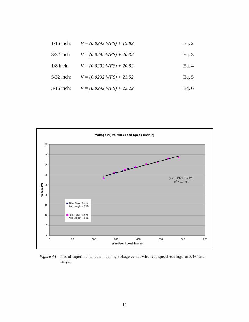
1/16 inch: V = (0.0292·WFS) + 19.82 Eq. 2
3/32 inch: V = (0.0292·WFS) + 20.32 Eq. 3
1/8 inch: V = (0.0292·WFS) + 20.82 Eq. 4
5/32 inch: V = (0.0292·WFS) + 21.52 Eq. 5
3/16 inch: V = (0.0292·WFS) + 22.22 Eq. 6
Voltage (V) vs. Wire Feed Speed (in/min)
y = 0.0292x + 22.22R2 = 0.9749
0
5
10
15
20
25
30
35
40
45
0 100 200 300 400 500 600 700
Wire Feed Speed (in/min)
Volta
ge (V
)
Fillet Size - 6mmArc Length - 3/16"
Fillet Size - 8mmArc Length - 3/16"
Figure 4A – Plot of experimental data mapping voltage versus wire feed speed readings for 3/16” arc length.
11
Arc Length Curves
20.00
22.00
24.00
26.00
28.00
30.00
32.00
34.00
36.00
38.00
40.00
42.00
0 100 200 300 400 500 600 700
Wire Feed Speed (in/min)
Volta
ge (V
Arc Length - 3/16)
Arc Length - 5/32Arc Length - 1/8Arc Length - 3/32Arc Length - 1/16
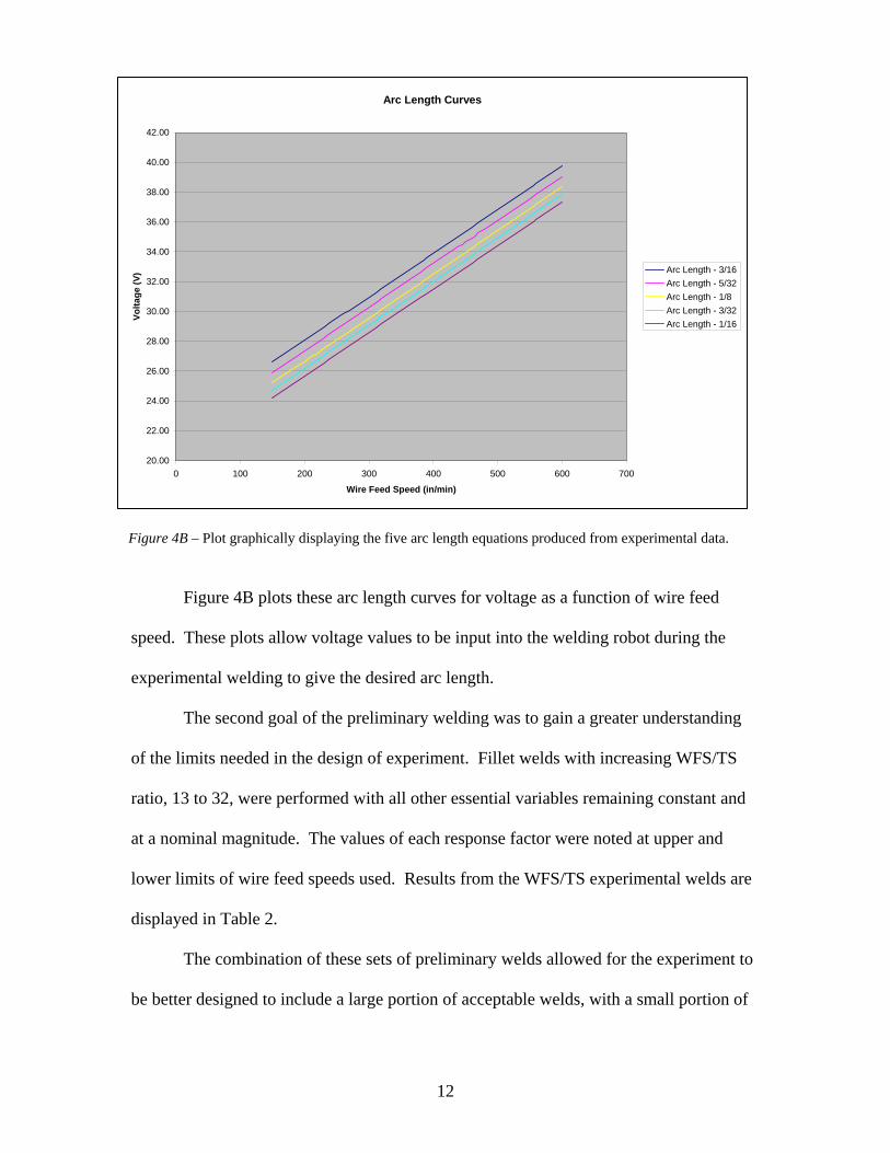
Figure 4B – Plot graphically displaying the five arc length equations produced from experimental data.
Figure 4B plots these arc length curves for voltage as a function of wire feed
speed. These plots allow voltage values to be input into the welding robot during the
experimental welding to give the desired arc length.
The second goal of the preliminary welding was to gain a greater understanding
of the limits needed in the design of experiment. Fillet welds with increasing WFS/TS
ratio, 13 to 32, were performed with all other essential variables remaining constant and
at a nominal magnitude. The values of each response factor were noted at upper and
lower limits of wire feed speeds used. Results from the WFS/TS experimental welds are
displayed in Table 2.
The combination of these sets of preliminary welds allowed for the experiment to
be better designed to include a large portion of acceptable welds, with a small portion of
12
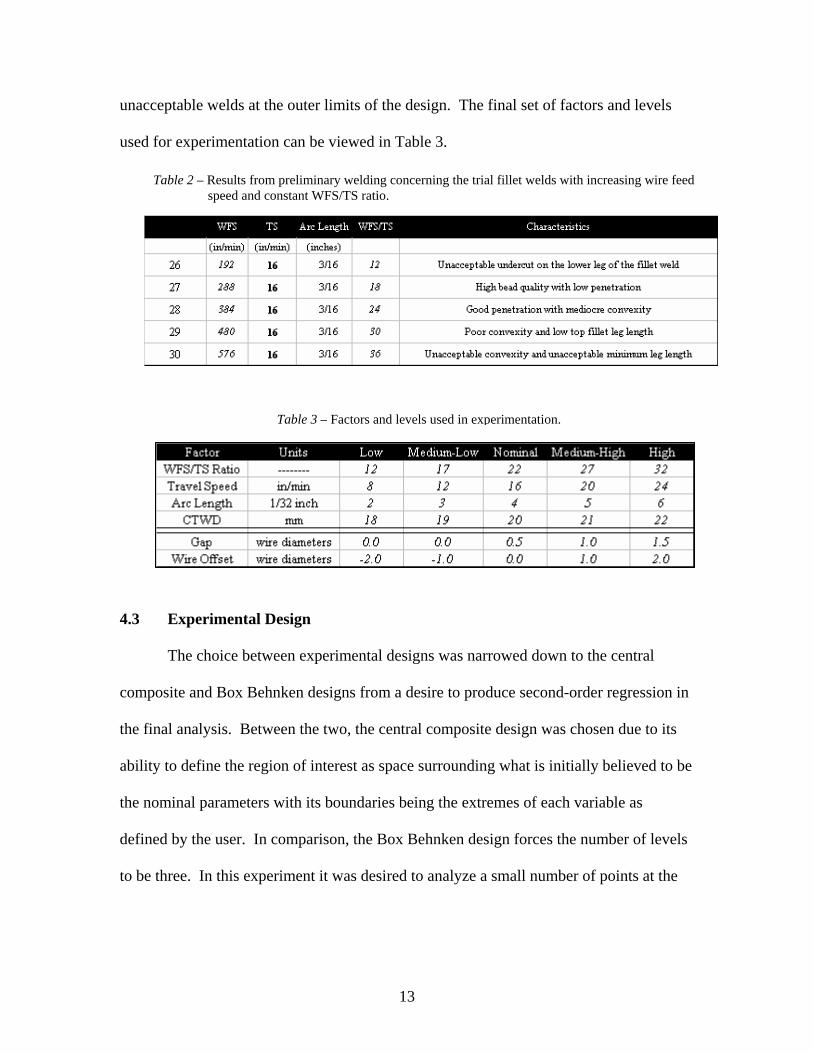
unacceptable welds at the outer limits of the design. The final set of factors and levels
used for experimentation can be viewed in Table 3.
Table 2 – Results from preliminary welding concerning the trial fillet welds with increasing wire feed speed and constant WFS/TS ratio.
Table 3 – Factors and levels used in experimentation.
4.3 Experimental Design
The choice between experimental designs was narrowed down to the central
composite and Box Behnken designs from a desire to produce second-order regression in
the final analysis. Between the two, the central composite design was chosen due to its
ability to define the region of interest as space surrounding what is initially believed to be
the nominal parameters with its boundaries being the extremes of each variable as
defined by the user. In comparison, the Box Behnken design forces the number of levels
to be three. In this experiment it was desired to analyze a small number of points at the
13

high and low ends of each variable range, and the central composite design allows for
this, while the Box Behnken experimental design does not.
The central composite structure is broken down into the center, factorial, and axial
points. As is expected the center points include the nominal values of each variable. The
factorial points on the other hand include those points that are neither nominal nor
extreme. In reference to Table 3, these values would be the medium-low and medium-
high values. The design structure is completed with the axial points which lie at the
extremes of the variable ranges. To minimize the number of experimental runs a half
design was chosen. This limited the number of interactions obtainable in the resulting
regression models, but it was assumed that the terms dropped did not have a strong
enough interaction to be included in the model. The central composite design resulted in
54 total runs, with 10 replicates taking place at the center point and two at the axial, or
star, points. Minitab 14, a statistical software tool, was utilized to develop the DOE. The
resulting total experimental array is displayed in Table 4.
14
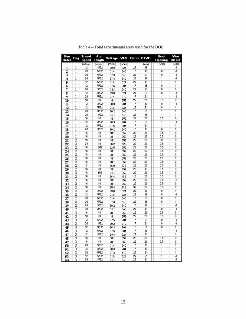
Table 4 – Total experimental array used for the DOE.
15
4.4 Experimental Welding
The welding was preformed at the Edison Joining and Technology Center (EJTC)
in The Ohio State University Welding Engineering Welding Process Laboratory using a
FANUC Robot ARCmate 100i welding robot and a Lincoln Electric 655 PowerWave
power supply. Fillet welds on twelve millimeter thick plates of A572 steel in the
horizontal, 2F, position were performed with an ER70S-6 electrode wire and utilizing 90-
10 Ar-CO2 shielding gas at 40 CFH. The 18 inch joint length allowed for three
experimental welds to be made per joint, as illustrated in Figure 5.
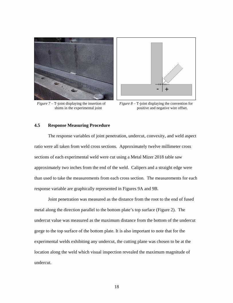
Fixturing was constructed in order to allow for precise and repeatable placement
of the joint on the work table, while also acting to prevent distortion during welding. The
fixturing utilized in this work is illustrated in Figure 6. Tack welds were made on the
ends of the joint following joint placement and clamping onto the makeshift fixture.
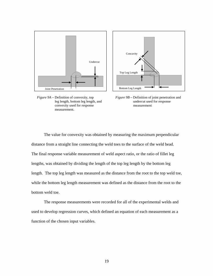
As displayed in Figure 7 Shims were placed in the joint before clamping and
tacking in order to incorporate the noise factor of root gap into the experiment. Four
shims were used on each T-joint, one on each end, and two separating the three
experimental welds. Extra tack welds were than added to the joint at each shim to ensure
that the gap width remained controlled.
The factor of weld offset was included in experimentation by moving the welding
electrode wire up to two wire diameters (0.052”) into and out of the joint. Figure 8
illustrates the coordinate system used to define placement of the wire prior to welding.
Positive displacement was taken to be displacement away from the joint, while negative
displacement was defined to be displacement into the joint.
16
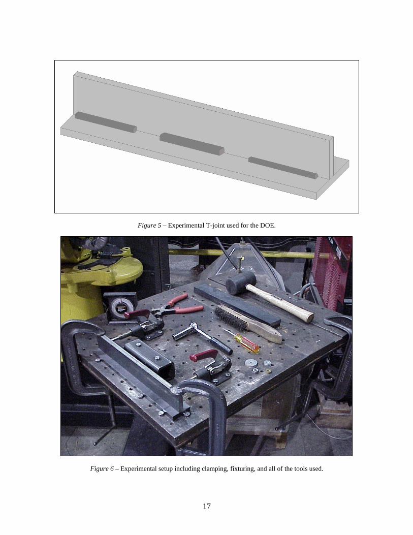
Figure 6 – Experimental setup including clamping, fixturing, and all of the tools used.
Figure 5 – Experimental T-joint used for the DOE.
17
+ -
Figure 7 – T-joint displaying the insertion of shims in the experimental joint
Figure 8 – T-joint displaying the convention for positive and negative wire offset.
4.5 Response Measuring Procedure
The response variables of joint penetration, undercut, convexity, and weld aspect
ratio were all taken from weld cross sections. Approximately twelve millimeter cross
sections of each experimental weld were cut using a Metal Mizer 2018 table saw
approximately two inches from the end of the weld. Calipers and a straight edge were
than used to take the measurements from each cross section. The measurements for each
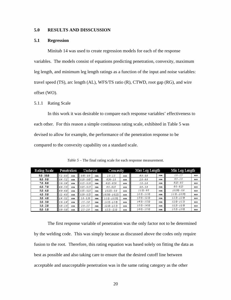
response variable are graphically represented in Figures 9A and 9B.
Joint penetration was measured as the distance from the root to the end of fused
metal along the direction parallel to the bottom plate’s top surface (Figure 2). The
undercut value was measured as the maximum distance from the bottom of the undercut
gorge to the top surface of the bottom plate. It is also important to note that for the
experimental welds exhibiting any undercut, the cutting plane was chosen to be at the
location along the weld which visual inspection revealed the maximum magnitude of
undercut.
18
Concavity
Top Leg Length
Bottom Leg Length Joint Penetration
Undercut
The value for convexity was obtained by measuring the maximum perpendicular
distance from a straight line connecting the weld toes to the surface of the weld bead.
The final response variable measurement of weld aspect ratio, or the ratio of fillet leg
lengths, was obtained by dividing the length of the top leg length by the bottom leg
length. The top leg length was measured as the distance from the root to the top weld toe,
while the bottom leg length measurement was defined as the distance from the root to the
bottom weld toe.
The response measurements were recorded for all of the experimental welds and
used to develop regression curves, which defined an equation of each measurement as a
function of the chosen input variables.
Figure 9A – Definition of convexity, top leg length, bottom leg length, and convexity used for response measurement.
Figure 9B – Definition of joint penetration and undercut used for response measurement
19
5.0 RESULTS AND DISSCUSSION
5.1 Regression
Minitab 14 was used to create regression models for each of the response
variables. The models consist of equations predicting penetration, convexity, maximum
leg length, and minimum leg length ratings as a function of the input and noise variables:
travel speed (TS), arc length (AL), WFS/TS ratio (R), CTWD, root gap (RG), and wire
offset (WO).
5.1.1 Rating Scale
In this work it was desirable to compare each response variables’ effectiveness to
each other. For this reason a simple continuous rating scale, exhibited in Table 5 was
devised to allow for example, the performance of the penetration response to be
compared to the convexity capability on a standard scale.
Table 5 – The final rating scale for each response measurement.
The first response variable of penetration was the only factor not to be determined
by the welding code. This was simply because as discussed above the codes only require
fusion to the root. Therefore, this rating equation was based solely on fitting the data as
best as possible and also taking care to ensure that the desired cutoff line between
acceptable and unacceptable penetration was in the same rating category as the other
20
variables. In result, it was determined that any penetration above 4.8 mm, (Rating 6.0 –
7.0), would be acceptable while any rating below was deemed unacceptable.
The rest of the response rating equations were based on D14.3: Specification for
Welding Earthmoving and Construction Equipment. The first of these variables,
undercut, is limited to a value no greater than 0.25 mm. Therefore, this rating was
divided among the highest and lowest values found from experimentation and placed
0.25 mm at the bottom end of the 6.0 -7.0 rating range.6
The limiting factor for the convexity rating was similar to undercut in the sense
that no value could exceed a certain maximum limit, but different in the aspect that this
maximum limit was a function of maximum leg length, as displayed in Equation 7. The
cutoff value is 0.0 mm because this rating stems from a difference between the limiting
number and the actual measurement. If the value is positive the convexity is less than the
limit. If the difference is negative than the convexity is over the limit and is thus deemed
unacceptable.
Maximum Convexity = (0.1 · maximum leg length) + 0.3 mm Eq. 7,6
The final response variables of maximum and minimum leg length were both
determined by taking the difference of the actual measured lengths to the limiting factors
determined by code. Equations 8 and 9 display both of the limiting values as determined
by code.
Maximum Leg Length = Nominal Leg Length + 3.2 mm Eq. 8,6
Minimum Leg Length = Nominal Leg Length – 0.8 mm Eq. 9,6
21
The nominal leg length used is the equations above are determined from the WFS/TS
ratio. Also, because the rating result is taken from a difference between a limiting
number and the actual measure, the cutoff value, like convexity, is 0.0 mm.
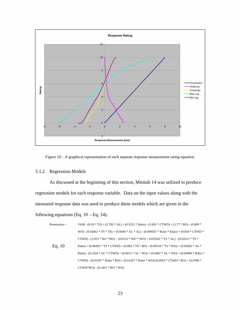
The final rating scale for the response variables is displayed in Table 5. It should
be noted that while the penetration scale is linear, each of the other variables is defined
by a nonlinear scale. This was necessary to allow for each cutoff value to be placed at
the same rating value while also properly fitting each scale to represent the data taken in
experimentation. Figure 10 plots each rating scale illustrating the linearity of the
penetration scale and the nonlinearity of the other variable rating scales.
The rating scale adopted allows the user to numerically define the boundary
between acceptable and unacceptable welds while also providing insight beyond this
distinction. The ratings give an understanding as to the degree of effectiveness or
defectiveness with each response along with the go or no-go determination. Also, the
quality issues included are all judged according to welding specification and code. This
adds to the credibility of the process being developed.
22
Response Rating
-2
0
2
4
6
8
10
12
-8 -6 -4 -2 0 2 4 6 8 10
Response Measurement (mm)
Rat
ing
PenetrationUndercutConcavityMax LegMin Leg
Figure 10 – A graphical representation of each separate response measurement rating equation.
5.1.2 Regression Models
As discussed at the beginning of this section, Minitab 14 was utilized to produce
regression models for each response variable. Data on the input values along with the
measured response data was used to produce these models which are given in the
following equations (Eq. 10 – Eq. 14).
Penetration = 19.69 - (0.18 * TS) + (2.783 * AL) + (0.3531 * Ratio) - (2.691 * CTWD) + (1.77 * RO) - (0.869 *
WO) - (0.02661 * TS * TS) + (0.0446 * AL * AL) - (0.009567 * Ratio * Ratio) + (0.039 * CTWD *
CTWD) - (1.053 * RO * RO) - (0.0132 * WO * WO) + (0.03545 * TS * AL) - (0.02511 * TS *
Ratio) + (0.08382 * TS * CTWD) + (0.085 * TS * RO) - (0.09518 * TS * WO) + (0.04582 * AL *
Ratio) - (0.2424 * AL * CTWD) + (0.6015 * AL * RO) + (0.0402 * AL * WO) + (0.03006 * Ratio *
CTWD) - (0.03187 * Ratio * RO) + (0.01427 * Ratio * WO)-(0.0919 * CTWD * RO) + (0.0789 *
CTWD*WO) - (0.5451 * RO * WO)
Eq. 10
23
Undercut = 156.2 + (0.812 * TS) - (11.825 * AL) + (1.399*Ratio) - (16.26 * CTWD) + (58.19*RO) -
(10.073*WO) - (0.0337 * TS * TS) + (0.4692 * AL * AL) - (0.01646 * Ratio * Ratio) + (0.4692 *
CTWD * CTWD) - (5.17 * RO * RO) + (0.4692 * WO * WO) + (0.0666 * TS * AL) + (0.03874 *
TS * Ratio) - (0.0528 * TS * CTWD) - (0.1056 * TS * RO) + (0.0579 * TS * WO) + (0.04636 *
AL * Ratio) + (0.2762 * AL * CTWD) + (0.5524 * AL * RO) + (0.7748 * AL * WO) - (0.05741 *
Ratio * CTWD) - (0.1148 * Ratio * RO) + (0.05328 * Ratio * WO) - (2.546 * CTWD * RO) +
(0.222 * CTWD * WO) + (0.4439 * RO * WO)
Eq. 11
Convexity = 60.5 - (0.979 * TS) - (12.679 * AL) - (1.365 * Ratio) - (1.02 * CTWD) + (16.27 * RO) + (4.36 *
WO) + (0.03154 * TS * TS) + (0.4906 * AL * AL) - (0.02088 * Ratio * Ratio) - (0.0235 * CTWD *
CTWD) + (1.369 * RO * RO) + (0.3455 * WO * WO) + (0.03724 * TS * AL) + (0.01048 * TS *
Ratio) - (0.03574 * TS * CTWD) - (0.101 * TS * RO) + (0.15331 * TS * WO) + (0.0798 * AL *
Ratio) + (0.3501 * AL * CTWD) - (0.7959 * AL * RO) + (0.0056 * AL * WO) + (0.08079 * Ratio *
CTWD) + (0.058 * Ratio * RO) + (0.03457 * Ratio * WO) - (0.7181 * CTWD * RO) - (0.3545 *
CTWD * WO) - (0.0065 * RO * WO)
Eq. 12
Maximum Leg Length = 75.99 - (0.2231 * TS) + (0.699 * AL) - (0.9584 * Ratio) - (5.617 * CTWD) - (1.307 *
RO) - (1.644 * WO) - (0.011487 * TS * TS) - (0.1705 * AL * AL) + (0.007047 * Ratio
* Ratio) + (0.1189 * CTWD * CTWD) + (0.1429 * RO * RO) - (0.0823 * WO * WO) +
(0.04067 * TS * AL) - (0.002554 * TS * Ratio) + (0.02261 * TS * CTWD) + (0.00466
* TS * RO) - (0.07017 * TS * WO) + (0.02099 * AL * Ratio) - (0.0378 * AL * CTWD)
+ (0.3315 * AL * RO) + (0.0829 * AL * WO) + (0.03051 * Ratio * CTWD) + (0.04917 *
Ratio * RO) - (0.02608 * Ratio * WO) - (0.058 * CTWD * RO) + (0.1331 * CTWD *
WO) - (0.32 * RO * WO)
Eq. 13
Minimum Leg Length = 164.9 - (0.552 * TS) - (8.117 * AL) - (0.886 * Ratio) - (12.76 * CTWD) - (0.22 * RO) -
(4.478 * WO) + (0.00368 * TS * TS) + (0.1662 * AL * AL) + (0.01079 * Ratio * Ratio)
+ (0.2892 * CTWD * CTWD) + (0.416 * RO * RO) + (0.0708 * WO * WO) + (0.07238
* TS * AL) + (0.0052 * TS * Ratio) - (0.01326 * TS * CTWD) + (0.0558 * TS *
RO) - (0.03735 * TS * WO) - (0.0321 * AL * Ratio) + (0.3105 * AL * CTWD) - (0.169
* AL * RO) + (0.0416 * AL * WO) + (0.01401 * Ratio * CTWD) - (0.0244 * Ratio *
RO) + (0.08002 * Ratio * WO) - (0.0506 * CTWD * RO) + (0.1184 * CTWD * WO) +
(0.395 * RO * WO)
Eq. 14
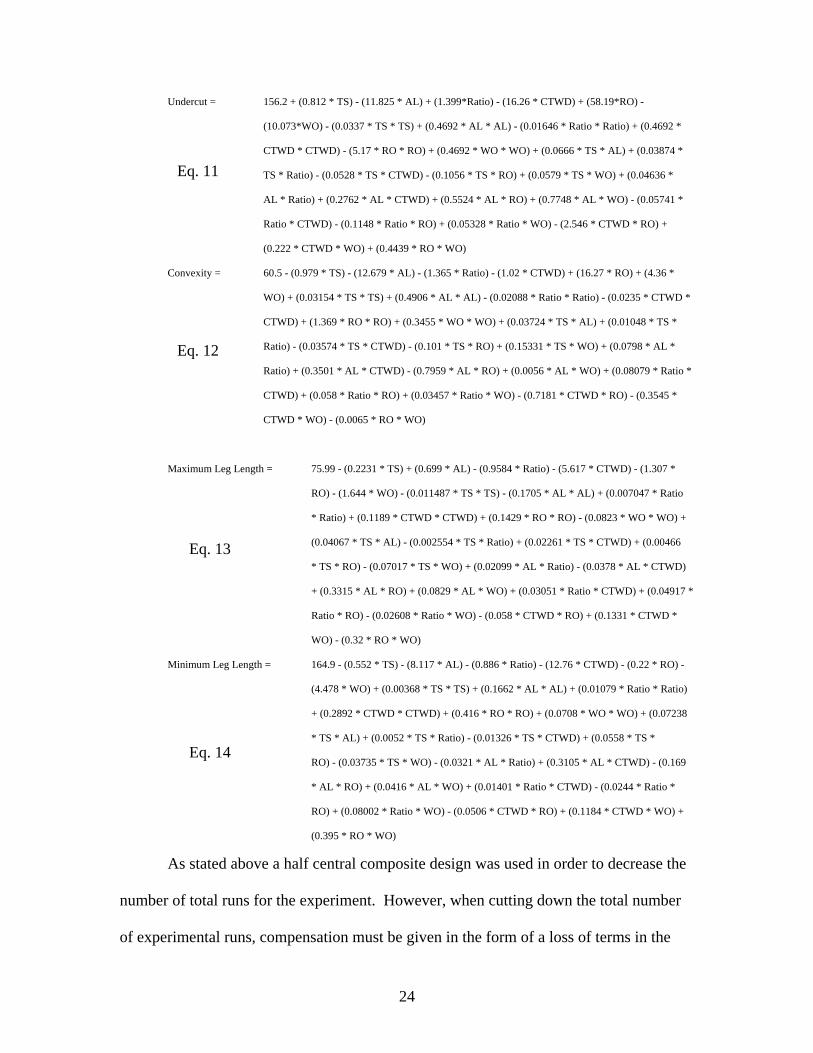
As stated above a half central composite design was used in order to decrease the
number of total runs for the experiment. However, when cutting down the total number
of experimental runs, compensation must be given in the form of a loss of terms in the
24
produced regression models. For this reason the three, four, five, and six order terms
have been eliminated from the regression models on the assumption that their impact was
less significant than the first and second order terms.
5.2 Contour Plots
The regression models displayed above all contain twenty-eight terms, one
coefficient constant term, six first order terms, and twenty-one second order terms. The
complexity, or simply the vast abundance of terms results in the need for a more clear,
and distinctive method of describing the relationships developed above.
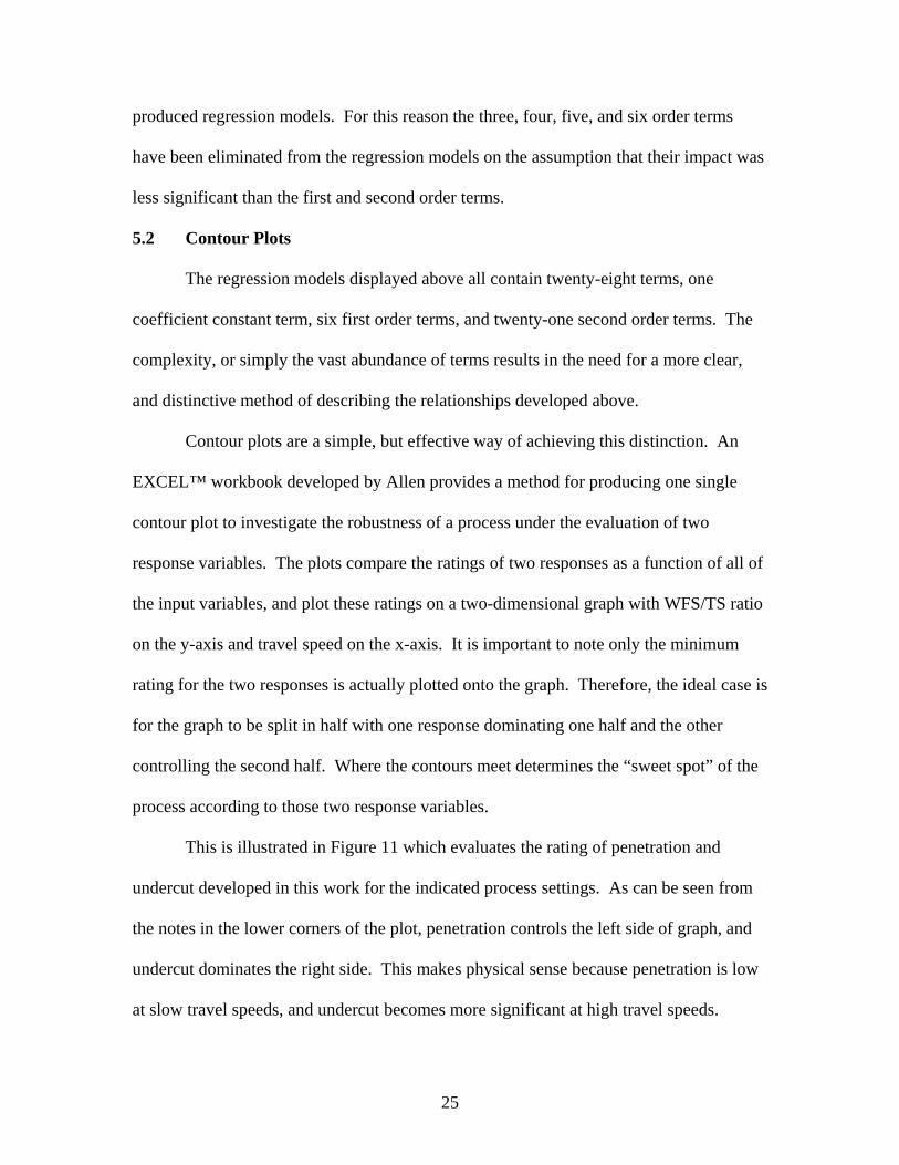
Contour plots are a simple, but effective way of achieving this distinction. An
EXCEL™ workbook developed by Allen provides a method for producing one single
contour plot to investigate the robustness of a process under the evaluation of two
response variables. The plots compare the ratings of two responses as a function of all of
the input variables, and plot these ratings on a two-dimensional graph with WFS/TS ratio
on the y-axis and travel speed on the x-axis. It is important to note only the minimum
rating for the two responses is actually plotted onto the graph. Therefore, the ideal case is
for the graph to be split in half with one response dominating one half and the other
controlling the second half. Where the contours meet determines the “sweet spot” of the
process according to those two response variables.
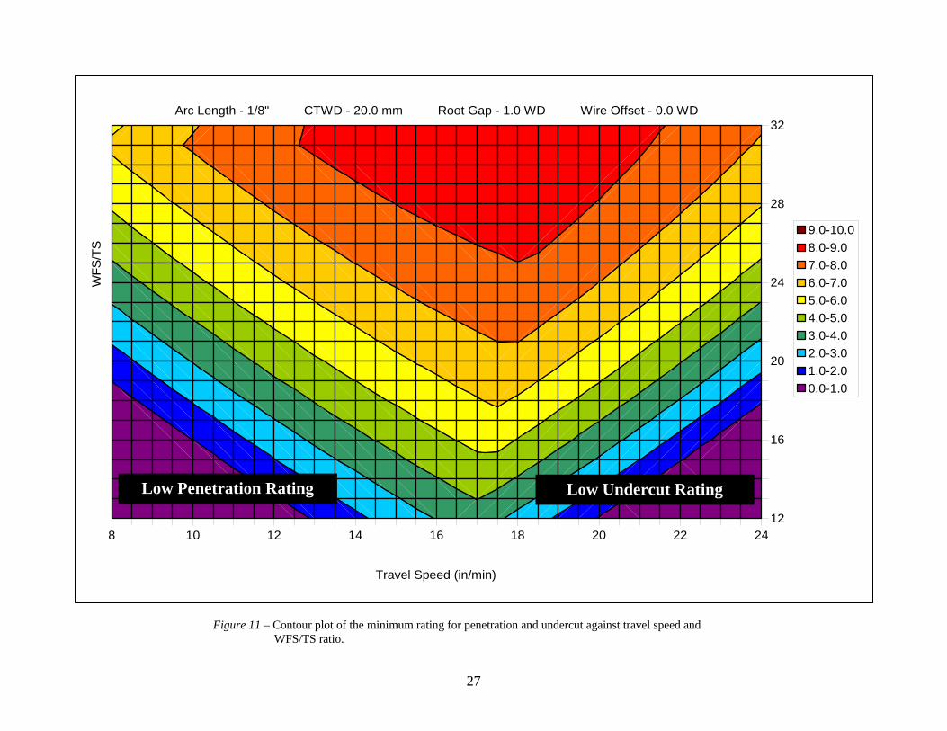
This is illustrated in Figure 11 which evaluates the rating of penetration and
undercut developed in this work for the indicated process settings. As can be seen from
the notes in the lower corners of the plot, penetration controls the left side of graph, and
undercut dominates the right side. This makes physical sense because penetration is low
at slow travel speeds, and undercut becomes more significant at high travel speeds.
25
26
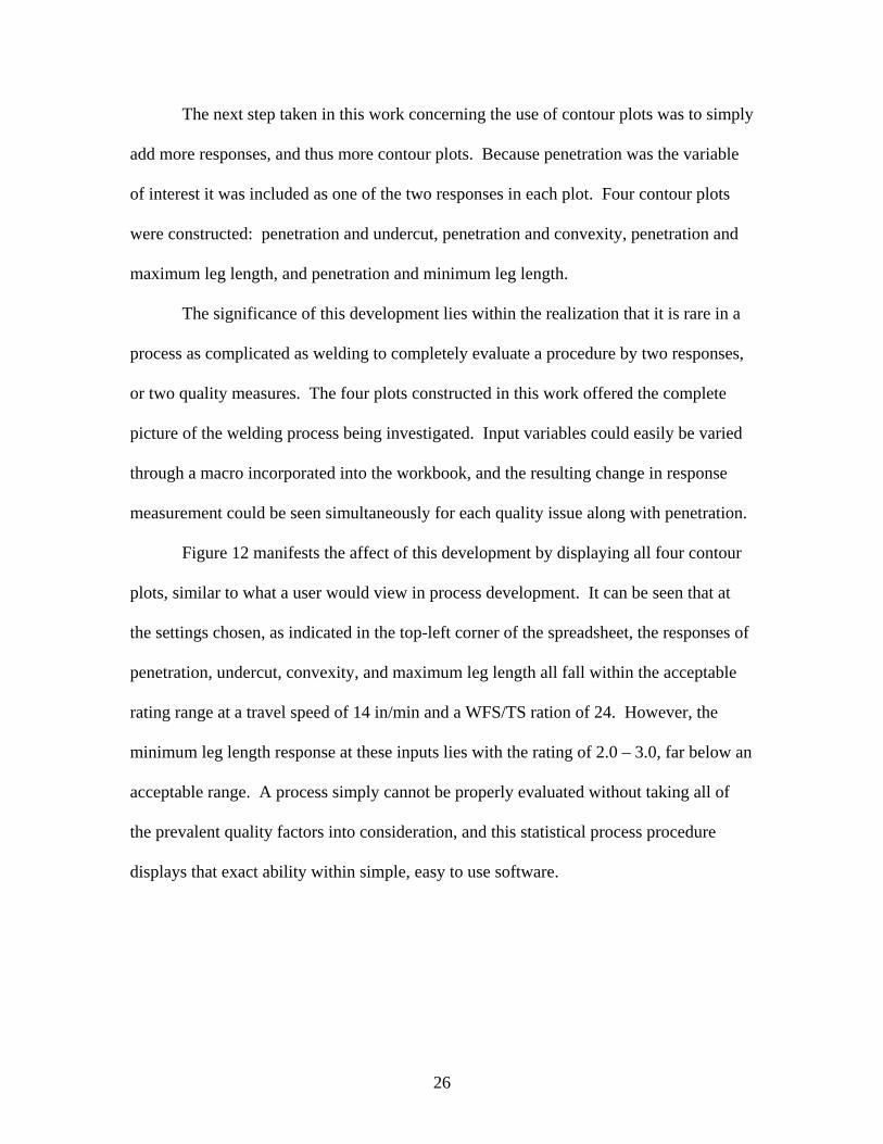
The next step taken in this work concerning the use of contour plots was to simply
add more responses, and thus more contour plots. Because penetration was the variable
of interest it was included as one of the two responses in each plot. Four contour plots
were constructed: penetration and undercut, penetration and convexity, penetration and
maximum leg length, and penetration and minimum leg length.
The significance of this development lies within the realization that it is rare in a
process as complicated as welding to completely evaluate a procedure by two responses,
or two quality measures. The four plots constructed in this work offered the complete
picture of the welding process being investigated. Input variables could easily be varied
through a macro incorporated into the workbook, and the resulting change in response
measurement could be seen simultaneously for each quality issue along with penetration.
Figure 12 manifests the affect of this development by displaying all four contour
plots, similar to what a user would view in process development. It can be seen that at
the settings chosen, as indicated in the top-left corner of the spreadsheet, the responses of
penetration, undercut, convexity, and maximum leg length all fall within the acceptable
rating range at a travel speed of 14 in/min and a WFS/TS ration of 24. However, the
minimum leg length response at these inputs lies with the rating of 2.0 – 3.0, far below an
acceptable range. A process simply cannot be properly evaluated without taking all of
the prevalent quality factors into consideration, and this statistical process procedure
displays that exact ability within simple, easy to use software.
8 10 12 14 16 18 20 22 2412
16
20
24
28
32
9.0-10.08.0-9.07.0-8.06.0-7.05.0-6.04.0-5.03.0-4.02.0-3.01.0-2.00.0-1.0
WFS
/TS
Travel Speed (in/min)
Arc Length - 1/8" CTWD - 20.0 mm Root Gap - 1.0 WD Wire Offset - 0.0 WD
Low Penetration Rating Low Undercut Rating
Figure 11 – Contour plot of the minimum rating for penetration and undercut against travel speed and WFS/TS ratio.
27
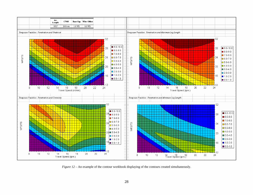
Figure 12 – An example of the contour workbook displaying of the contours created simultaneously.
28
5.3 Optimization
The optimization process used in this work looked to meet the needs of industry
by providing a tool for maximizing travel speed while avoiding certain limits for quality
or dimensional values. In this case the limiting factors for travel speed were penetration
along with the quality factors of undercut, convexity, and maximum and minimum fillet
leg. The rating scale used in the regression and contour plots (Table 5) was developed
not only to allow for comparison among the response factors, but also to set in place a
distinct cut off rating for acceptable welds. This lower specification limit (LSL) was set
to be the rating of 6.0. Therefore, the LSL used in optimization was obviously chosen to
be a rating of 6.0 for each of the constraining variables.
For the actual optimization a spreadsheet was developed utilizing the EXCEL™
solver to find the maximum travel speed for six typical sets of root gap and wire offset
values. These sets of noise variables act to incorporate the industrial environment into
the optimization. The solver program varied each of the controllable input variables
(travel speed, arc length, WFS/TS ratio, and CTWD), producing the values for each
variable that results in the maximum travel speed for the set of defined noise variables.
The constraints on this optimization included holding the resulting response rating at or
above 6.0 for each set of noise variables, along with restricting the input variables inside
of the space defined in experimentation. The addition of extra responses, again, helps in
the overall procedure development by allowing the process to be optimized over all of the
prevalent quality issues.
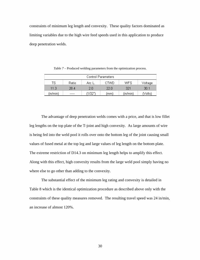
The resulting welding procedure is listed in Table 7, and is highlighted by a low
travel speed of 11.3 in/min. The slow travel speed produced resulted chiefly from the
29
constraints of minimum leg length and convexity. These quality factors dominated as
limiting variables due to the high wire feed speeds used in this application to produce
deep penetration welds.
Table 7 – Produced welding parameters from the optimization process.
The advantage of deep penetration welds comes with a price, and that is low fillet
leg lengths on the top plate of the T-joint and high convexity. As large amounts of wire
is being fed into the weld pool it rolls over onto the bottom leg of the joint causing small
values of fused metal at the top leg and large values of leg length on the bottom plate.
The extreme restriction of D14.3 on minimum leg length helps to amplify this effect.
Along with this effect, high convexity results from the large weld pool simply having no
where else to go other than adding to the convexity.
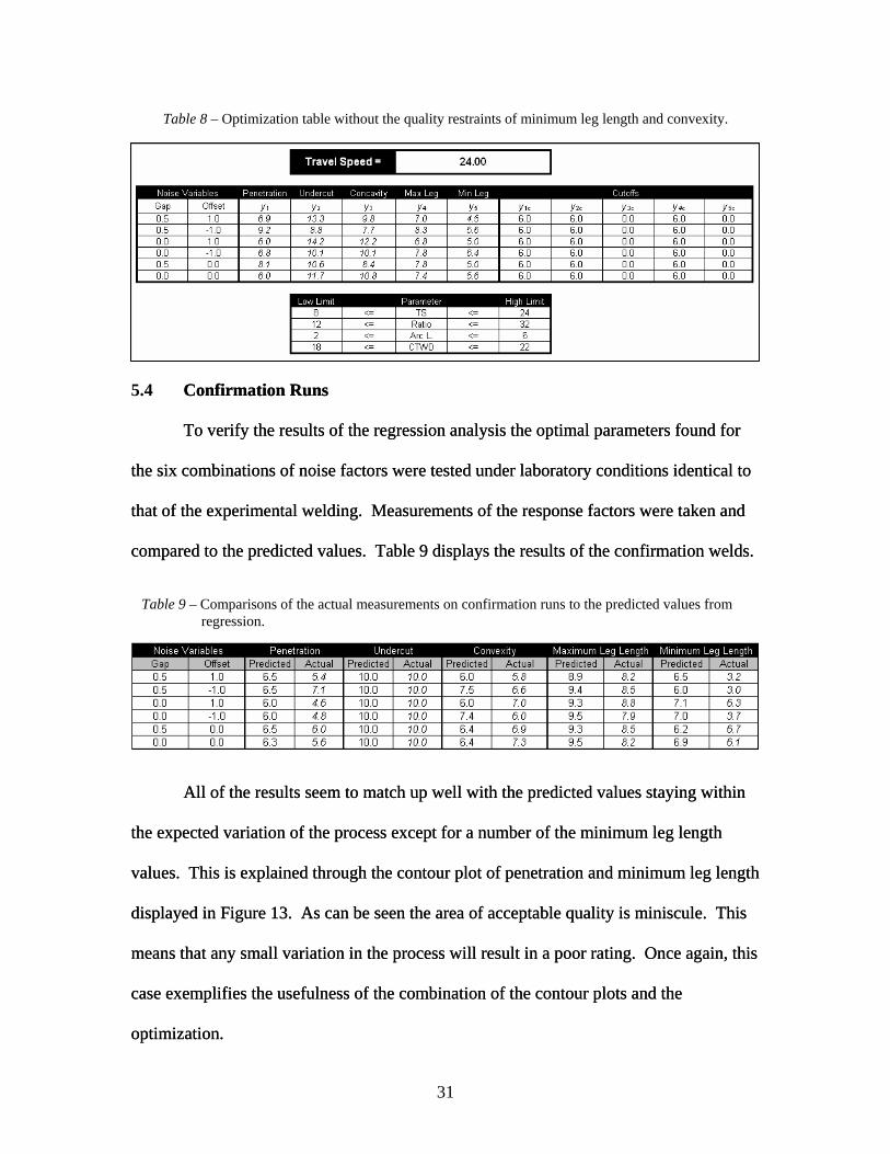
The substantial effect of the minimum leg rating and convexity is detailed in
Table 8 which is the identical optimization procedure as described above only with the
constraints of these quality measures removed. The resulting travel speed was 24 in/min,
an increase of almost 120%.
30
31
Table 8 – Optimization table without the quality restraints of minimum leg length and convexity.
5.4 Confirmation Runs Confirmation Runs
To verify the results of the regression analysis the optimal parameters found for
the six combinations of noise factors were tested under laboratory conditions identical to
that of the experimental welding. Measurements of the response factors were taken and
compared to the predicted values. Table 9 displays the results of the confirmation welds.
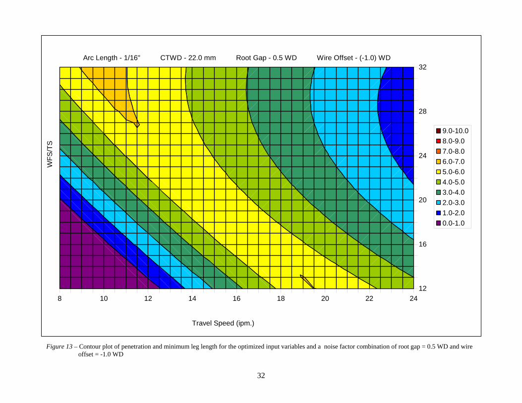
All of the results seem to match up well with the predicted values staying within
the expected variation of the process except for a number of the minimum leg length
values. This is explained through the contour plot of penetration and minimum leg length
displayed in Figure 13. As can be seen the area of acceptable quality is miniscule. This
means that any small variation in the process will result in a poor rating. Once again, this
case exemplifies the usefulness of the combination of the contour plots and the
optimization.
Table 9 – Comparisons of the actual measurements on confirmation runs to the predicted values from regression.
32
8 10 12 14 16 18 20 22 2412
16
20
24
28
32
9.0-10.08.0-9.07.0-8.06.0-7.05.0-6.04.0-5.03.0-4.02.0-3.01.0-2.00.0-1.0
WFS
/TS
Travel Speed (ipm.)
Arc Length - 1/16" CTWD - 22.0 mm Root Gap - 0.5 WD Wire Offset - (-1.0) WD
Figure 13 – Contour plot of penetration and minimum leg length for the optimized input variables and a noise factor combination of root gap = 0.5 WD and wire offset = -1.0 WD
4.0 CONCLUSIONS
The conclusions for this work include the main results concerning the
development with the statistical process design along with the outcomes for the
application, and are listed in the following:
Statistical process design procedure
• This process design can successfully adapt to multiple response variables.
– Including all of the significant variables allows the user to simultaneously view the effects of varying input variables on output responses.
– A greater benefit is found in optimizing over all of the critical quality measurements.
• Basing the rating system allows for simple setup of the scale along with easy
interpretation of acceptable and unacceptable welds.
Application
• The process for deep penetration GMAW does not exhibit full robustness
according to D14.3 welding code.
• More research is needed in decreasing convexity and increasing the top fillet leg
length while maintaining the penetration results found in this work.
5.0 FUTURE WORK
The further development of a statistical process design for robotic gas metal arc
welding performed in this work was an extension of research performed by Allen et al in
2002. The success found here however, does not mean that opportunities for further
advancement are nonexistent. While this work verified its ability to perform under a new
joint and weld type, and different response variables there are more options for
expansion. Submerged Arc Welding (SAW) and robotic Gas Tungsten Arc Welding
32
(GTAW) are possible untested process applications, while porosity measurements, weld
strength, and weld toe radius are possible response factors.
Along with new processes and variables further study includes developing a
method for comparing response variables without a common rating scale. The
introduction of a rating scale amplifies the complexity of the process while also
weakening its continuity.
Finally, further development needs to take place concerning a standard method for
running the preliminary experimental welds. These are crucial to defining the limits of
the main DOE along with picking out the pertinent response variables, and thus vital to
the overall success of the experiment within the shortest amount of time.
6.0 ACKNOWLEDGEMENTS
I would like to thank Professor Richard Richardson of The Ohio State University
Industrial Welding and Systems Engineering (IWSE) department for his guidance and
support throughout this work. His input was invaluable and greatly appreciated. I would
also like to acknowledge the assistance given by Professor Theodore Allen of the IWSE
department at Ohio State for all of his contributions concerning the development of the
contour plots and the optimization process.
I would also like to acknowledge the assistance of Cory Reynolds, Engineering
Supervisor, with John Deere Dubuque Works. The support from Cory Reynolds and
Deere & Company allowed this study to be performed and completed with success.
Finally, I would like to thank Brent Holloway for his assistance throughout the
project. His help ranged from aiding in fabrication of the tungsten pointer to the shearing
33

of shim pieces to produce controlled gaps for experimentation. His support significantly
decreased to total project time.
34
7.0 REFERENCES
1 The Procedure Handbook of Arc Welding, The James F. Lincoln Arc Welding
Foundation. 14th edition. 2000. pp.1.1-8 – 1.10.
2 Genichi Taguchi, Shin Taguchi, Subir Chowdhury. Robust Engineering.
McGraw-Hill: New York, NY, 2000.
3 D. Harwig. “Weld Parameter Development of Robot Welding.” Technical Paper
for the Society of Manufacturing Engineers. September, 1996.
4 D.C. Montgomery. Design and Analysis of Industrial Experiments. Fifth Edition.
John Wiley and Sons. New York, NY. 1995.
5 T.T Allen, R.W. Richardson, D. P. Tagliabue, and G.P Maul. “A Statistical
Process Design Procedure for the Arc Welding of Sheet Metal.” Welding Journal,
May 2002.
6 C. L. Ribardo. “Desirability Functions for Comparing Arc Welding Parameter
Optimization Methods and for Addressing Process Variability Under Six Sigma
Assumptions.” Dissertation. The Ohio State University. 2000.
7 AWS D14.3 Specification for Welding Earthmoving and Construction
Equipment. American Welding Society: Miami, FL, 2000.
8 Private Communication. Cory Reynolds, Senior Engineer Manufacturing
Technology, Deere & Company.
9 Welding Handbook, The American Welding Society. Vol. 2. 8th Edition. 1991.
pp. 110-154
35
Recommended