Mathematical Statistics
Stockholm University
Unallocated Loss Adjustment ExpenseReserving
Esbjorn Ohlsson
Research Report 2013:9
ISSN 1650-0377

Postal address:Mathematical StatisticsDept. of MathematicsStockholm UniversitySE-106 91 StockholmSweden
Internet:http://www.math.su.se/matstat

Mathematical StatisticsStockholm UniversityResearch Report 2013:9,http://www.math.su.se/matstat
Unallocated Loss Adjustment ExpenseReserving
Esbjorn Ohlsson∗
December 2013
Abstract
In non-life insurance the provision for outstanding claims (theclaims reserve) should include future loss adjustment expenses, i.e. ad-ministrative expenses to settle the claims, and therefore we have to es-timate the expected Unallocated Loss Adjustment Expenses (ULAE) –expenses that are not attributable to individual claims, such as salariesat the claims handling department. The ULAE reserve has receivedlittle attention from European actuaries in the literature, supposedlybecause of the lack of detailed data for estimation and evaluation.Having good estimation procedures will, however, become even moreimportant with the introduction of the Solvency II regulations, thatrequire unbiased estimation of future cash flows for all expenses. Wepresent a model for ULAE at the individual claim level that includesboth fixed and variable costs. This model leads to an estimate ofthe ULAE reserve at the aggregate (line-of-business) level, as demon-strated in a numerical example from a Swedish non-life insurer.
KEY WORDS: Unallocated Loss Adjustment Cost, Claims HandlingExpenses, Reserving, Paid-to-Paid method, Solvency II.
∗Lansforsakringar Alliance and Mathematical Statistics, Stockholm University, Sweden.E-mail: [email protected].

1 Introduction
In non-life insurance the provision for outstanding claims (the claims reserve)
should include future loss adjustment expenses, i.e. administrative expenses
to settle the claims, for incurred claims, whether reported or not. Some of
these expenses are attributable to individual claims and are often registered
in the claims handling system. This part of the expenses is called Allocated
Loss Adjustment Expenses (ALAE) and typically include external costs for
lawyers or other expertise. For actuarial purposes, ALAE are thus contained
in the claims figures and the provision for such costs is estimated together
with the direct claim costs and require no special treatment. The rest of the
adjustment costs are called Unallocated Loss Adjustment Expenses (ULAE)
and typically consist of internal costs, mainly salaries at the claims handling
department, together with their share of overhead costs, such as IT, manage-
ment and premises costs. These costs are not only impossible to attribute to
individual claims, but can neither be segmented at the granularity necessary
to include them in claims triangles or other data used in traditional claims
reserving. Therefore, the ULAE reserve (the provision for ULAE) has to be
estimated separately and added to the provision for claim costs.
Note that the Claims reserving manual of the Institute of Actuaries (1997)
uses the notation direct and indirect expenses while we have chosen the US
terms ALAE and ULAE here.
Spalla (2001) notes that the distinction between ALAE and ULAE may be
different at different companies, and reports that in the US there was a rec-
2

ommendation in 1998 on how to distinguish the two, with the objective of
consistent reporting. Under the forthcoming European Solvency II regula-
tions, the Best Estimate should contain all future expenses, without any
explicit distinction between ALAE and ULAE. We follow this line and con-
sider the ULAE reserve only as an operative means of covering expenses not
already taken care of by the estimation of claim costs based on data from
the claim systems. Hence, our distinction between ALAE and ULAE is just
a question of how the data is organized, whith far-reaching implications on
the methods for estimation. This implies that the split between ALAE and
ULAE may differ between companies, but consistency between their report-
ing can nevertheless be achieved at the level of the total claims reserve.
The ULAE reserve has received little attention in the literature by Euro-
pean actuaries, an exception being Buchwalder, Merz, Buhlmann & Wutrich
(2006). On the other hand, there are a number of papers from meetings of
the CAS (Casualty Actuarial Society) in the US; besides the already quoted
Spalla (2001) we like to mention Kittel (1981), Johnson (1989), Mango &
Allen (1999) and Conger & Nolibos (2003). We refer the reader to these
papers for further references.
The reason for the low interest from actuarial science on the subject is pre-
sumably the lack of data to perform statistical estimation, further discussed
below. A consequence of the lack of data is also that methods can not be
tested against experience. As a result, the proposed methods are based on
assumptions and expert judgement that can not be verified empirically. Note
also that ULAE reserves typically consist of just 5-10 % of the total reserve,
3

which makes them much less important than the rest of the claims reserve,
while still by no means negligible.
Notwithstanding these facts, we believe that it is valuable to base the as-
sumptions and estimates on proper models, and this is even more so consid-
ering the requirements of Solvency II. The object of this paper is to present
a relatively general framework for making assumptions and estimating the
ULAE reserve, while keeping the estimate simple. This is done by intro-
ducing a micro-level (claim by claim) model, which is then estimated at the
aggregated level.
2 Available data
The starting point is the data on historical ULAE payments, which should
be available at least per accounting year. We will restrict our discussion
to the latest accounting year, but the methods can trivially be extended to
using data from several years or other periods. Last years observed ULAE
is denoted L here. It should be possible to divide this amount into lines of
business (LoB), with more or less accuracy, in which case the methods in this
paper should be read as relating to a single LoB and L is the ULAE in that
LoB.
The exact definition of L, e.g. in terms of which overhead expenses to include,
is of course very important. However, this issue is beyond the scope of the
present paper and we just assume that definition is already set, presumably
by regulation, and that we have a useful observation of L available. In the
4

words of Kittel (1981), the exact definition “does not matter” here, in spite
of its importance.
A precise estimate of future ULAE would require more detailed data than
just L. This could include separate costs for opening, maintaining and closing
claims, all preferably split by claim size and types of claims. Such data are
typically not available at a reasonable cost for the insurance companies. It
is hard to think of how they could be, unless the expenses were registered
on a case-by-case basis by the claim handlers, by e.g. noting the time used
for handling each claim, with overhead allocated proportionally. But if such
data was collected on a regular basis, the expenses would actually be allocated
and could be treated as ALAE.
Johnson (1989) mentions the possibility of performing a time study for a
temporary time period. Spalla (2001) discusses a study using data from
the claims handling systems on time spent on different activities and notes
that even with the use of such data “the project involved an investment of
significant resources. The cost of such an investment goes beyond the benefit
that would be derived by merely improving the accuracy of the estimation
of ULAE liabilities.” Indeed, the main justification for the mentioned study
was to improve product pricing, not the ULAE reserve. With this in mind,
we will assume here that no such study is available and we believe that this
is the typical case. Then the lack of detailed data for ULAE follows more or
less by definition, since expenses with detailed information at the claim level
would be classified as ALAE, as argued above. We call this the fundamental
lack of data for ULAE and this is the situation we discuss in the present
5

paper.
In contrast to the lack of detailed data for expenses, we will typically have
an actuarial database of insurances and claims, so that we can get detailed
data on the number and cost of different types of claims. Let us first look at
a traditional incremental claims triangle, in which Cij denotes the observed
paid claims for accident year i and development year j, i = 1, 2, . . . ,m;
j = 0, 1, . . . , J .
Table 2.1: Claims development triangle with J = m.
Accident Development yearyear 0 1 2 · · · J − 1 J
1 C10 C11 C12 · · · C1,J−1 C1,J
2 C20 C21 C22 · · · C2,J−1
3 C30 C31 C32 · · ·...
......
...m− 1 Cm−1,0 Cm−1,1
m Cm,0
Of special interest here is the paid claims during the latest accounting year
C =∑
i+j=mCij. We further assume that we have an estimate of the out-
standing claims, i.e. the sum of future Cij in the lower part of the triangle,
plus an eventual tail, computed by actuarial methods. Let us denote the
reserve for reported but not settled claims (RBNS) by R and the reserve for
incurred but not yet reported claims (IBNYR) by I. (We refrain from distin-
guishing between the quantity being predicted and the predictor here, since
we are not investigating any stochastic properties of these estimates, but
rather take them as given.) Note also that C, R and I should be given gross
6

of reinsurance, undiscounted and without risk margin our any other extra
margin that the company may hold for safety reasons, since these accounting
measures are unlikely to influence the ULAE cost.
In many cases, R is just taken to be the sum of the case reserves (individual
claims reserves), but it might be an estimate of the total cost for reported
claims, as in the method by Schnieper (1991). As for I, if an estimate of
IBNYR (“pure IBNR”) is not available, we might approximate it by the
difference between the actuary’s best estimate of the total reserve and case
reserves.
We also have the possibility to group the data by the opening and closing time
of the claim. Following Mango & Allen (1999) the claims that are handled
over the last accounting year are divided into four groups, here denoted B1–
B4.
Table 2.2: Sectioning of claims
End of the yearClosed Open
Beginning Not open B1 B3
of the year Open B2 B4
Here B1 is the set of claims that were opened and closed during the year,
irrespective of accident year, etc. The number of claims in group Bk is
denoted Ak, k = 1, 2, 3, 4, so that we have
We will also assume that we have an estimate of the number AI of unknown
claims. This can be achieved by a straight-forward triangulation of data on
7

Table 2.3: Number of claims in the groups
End of the yearClosed Open
Beginning Not open A1 A3
of the year Open A2 A4
the number of reported claims and will not be discussed further here.
We can also divide the paid claims during the year, C, into the same four
sections, so that C = C1 + C2 + C3 + C4.
Table 2.4: Paid claims within the groups
End of the yearClosed Open
Beginning Not open C1 C3
of the year Open C2 C4
3 The Paid-to-Paid method
Before presenting our model, we shall discuss the simple Paid-to-Paid (PTP)
method. This method is based on the observed ratio of loss adjustment cost
to amount paid, i.e. L/C. If this ratio is the same for the claims in the
reserve (R + I) as for those handled during the last accounting year, we get
the simplest form of PTP estimate of the ULAE reserve U as
U =L
C(R + I) (3.1)
Mango & Allen (1999), as well as Institute of Actuaries (1997), note that the
8

simple paid-to-paid estimate can be expected to be biased upwards:. While
the ULAE itself increases with claim size, the percentage of ULAE should
be a decreasing function of the claim size, and since claims that are closed
quickly tend to be smaller on the average than those that are open longer,
an upward bias will result.
As a remedy, it has been suggested to use some kind of “50/50 rule”: ap-
proximately 50 % of the ULAE cost is paid at the opening of the claim and
50 % at the closing. Johnson (1989) describe the “classical” 50/50 rule in
words as
U =L
C(R/2 + I) = L
R/2 + I
C1 + C2 + C3 + C4
(3.2)
and this is also the equation given in the Claims reserving manual by the
Institute of Actuaries (1997, Section K4) in the UK; in fact, this is the only
method mentioned for indirect expenses (ULAE) reserving there. This of
course results in a lower ULAE reserve than the basic PTP method
U =L
C(R + I) = L
R + I
C1 + C2 + C3 + C4
The description of the 50/50 rule in Mango & Allen (1999), like Johnson
(1989), is given without an explicit formula, but seems to imply
U = LR/2 + I
C1 + 12(C2 + C3)
(3.3)
Indeed, this seems more logical than (3.2) if the 50/50 rule applies, under
which C4 generates no ULAE and C2 and C3 only half as much as C1. Mathe-
matically, (3.3) is not always lower than the basic PTP, as seen by considering
the case I = 0, but it should result in a lower ULAE reserve in cases where I
9

is small relative to R and C1 > C4, as seen by setting I = 0 above. See also
Section 4.1 for the method of Kittel (1981) which is quite close to (3.3). We
conclude that the 50/50 rule in its two appearances is either not perfectly
logical or not fail-proof to give a reduction of the bias.
As an alternative to methods having paid amounts as exposure, one might
consider methods based on the number of claims. Conger & Nolibos (2003)
mention an early method by R. E. Brian where the ULAE is split into dif-
ferent types of transactions: setting up the claim, maintaining the claim,
etc. As discussed in the previous section, we do not assume such data to be
available here.
A method based on claim counts that is simpler to apply was given by John-
son (1989) and is based on the assumption that the ULAE cost is given by
a fixed amount each year the claim is open, with twice the cost during the
first year when the claim is opened. In our experience, this idea of the ULAE
being completely independent of the claims size is not quite realistic, but it
seems reasonable that part of the cost is a fixed amount per claim as in these
models. Therefore we will include a fixed, i.e. claim by claim, part of the
ULAE in of our method below.
4 A micro-level model combining payments
and claim numbers
Even if we do not have data on ULAE costs at the individual claim level, we
think that it is informative to start by deriving a model at that level.
10

It seems natural to assume that the ULAE for a claim is the combination
of a fixed cost, an ULAE per claim, and a cost proportional to the loss, an
ULAE per unit of paid loss. This suggests a regression type model
ui = α + βci, (4.1)
where ui is the ULAE for claim i, and ci is the paid claim cost for claim i, for
the time period considered. This might be the entire time for handling the
claim, but in our further specifications of the model below we will often refer
to the latest accounting year, but also consider the time from the accounting
date till the closing of the claim, i.e. the time during which we have a reserve
for the claim.
Equation (4.1) of course just specifies the expected value structure. It could
be made into a proper regression model by adding a stochastic error term,
but since we do not have data at this level, it is not very meaningful to do
so, cf. Buchwalder, Merz, Buhlmann & Wutrich (2006) who make a similar
remark for the presentation of the “New York” method.
As mentioned above, several authors suggest methods based on the obser-
vation that there might be a cost for opening and another for closing the
claim. In our model, this would imply that we should split the fixed part
into two. So, we introduce s as the proportion of the fixed ULAE cost α that
is incurred at the opening, 0 ≤ s ≤ 1, so that sα is the fixed cost for opening
a claim and (1− s)α the fixed cost for closing. There may of course also be a
fixed claims maintenance cost between opening and closing, but presumably
this is smaller than the others and in order to keep the model simple we will
11

ignore this.
We will write ui = u1i +u2i, where u1i is the fixed part and u2i is the variable
part of the ULAE for claim i. In the time perspective of the latest accounting
year, we then have
u1i =
α, if iεB1 i.e. opened and closed during the period;(1− s)α, if iεB2 i.e. open from the beginning and then closed;sα, if iεB3 i.e. opened during the period, but not closed;0, if iεB4 i.e. open during the entire period;
(4.2)
Aggregating this fixed cost model over all claims that have been open some
time during the last year, i.e. over B1 ∪B2 ∪B3 ∪B4, we get
L1 = α(A1 + (1− s)A2 + sA3), (4.3)
with L1 denoting the (unknown) fixed part of the ULAE for the last account-
ing year.
Note that if the entire ULAE cost would be fixed, then L1 = L and (4.3)
gives us a (simplistic) cost per unit model. In order to estimate α we will
have to make an assumption on the value of s. This might be done by expert
judgement, consulting the claim handling department, but as default we will
use the standard 50/50 rule, i.e. s = 0.50.
IF L1 was known, we could now estimate α by equating L1 to α(A1 + sA3 +
(1− s)A2), with the result
12

α =L1
A1 + sA3 + (1− s)A2
. (4.4)
If we were to use a pure fixed cost model, we should then apply this ULAE
per normalized claim, to the the claims reserve. We have A3+A4 open claims
in the reserve and an estimated number AI of unknown claims. The pure
fixed ULAE reserve is then
U1 = α((A3 + A4)(1− s) + AI) = L1(A3 + A4)(1− s) + AI
A1 + A3 s+ A2(1− s). (4.5)
where A1 − A4 can be computed from the claim files and as default we set
s = 0.50.
We now turn to the variable cost and go back to the individual claim level.
As already mentioned, there is reason to believe that the cost per paid unit β
is larger for small claims than for large ones. We do not always know which
claims will become large and which will be small, so instead of splitting the
claims by size, we recall the remark by Mango & Allen (1999) that claims
that are closed quickly are on the average smaller than those that are open
longer. Among B1 −B4, the first one consists of claims that are expected
to be closed more rapidly, but this fact can not be used to construct an
estimate since the proportions with with these claims are represented in the
claims reserve is unknown. Instead we single out the claims payments for
the current accident year, i.e. payments for claims incurred during the latest
accounting year, and denote them by B0. The payments for these claims
was denoted Cm,0 in the claims triangle in Table 2.1, but will here we write
13

C0 = Cm,0 for short. These payments should include a lot of small claims
that are quickly closed, even though of course we have a few large claims
here, too. In any case, we expect more small claims among those paid for
here than in the claims reserve, which does not contain any B0 type claims.
Let r, 0 ≤ r ≤ 1, denote how much less ULAE we expect per paid claim unit
in the rest of the payments as opposed to B0. To get the variable part of
the ULAE, we thus multiply ci by β if the claim belongs to B0 and multiply
it by rβ for all other claims.
The model for variable cost is then
u2i =
{βci, if iεB0 i.e. is incurred during the period;rβci, else.
(4.6)
By combining equations (4.2) and (4.6) we get our final model for individual
ULAE ui = u1i + u2i, being a generalization of (4.1). We now aggregate
the variable cost model (4.6) over all claims that have been open some time
during the last year. The result is
L2 = β(C0 + r(C − C0)) , (4.7)
with L2 denoting the (unknown) variable part of the ULAE for the last
accounting year. The payments C0 and C are easy to compute and if we
temporarily ignore that L2 and r are unknown, we get the estimate
β =L2
C0 + r(C − C0)(4.8)
Let us for a moment assume that the fixed cost is zero, so that L2 = L. If we
let r = 1 we are then back in the pure PTP method with β = L/C. Looking
14

for a default value of r less than 1, we again revert to something similar to
a 50/50 rule, and choose r = 0.5, well aware that this is not really a 50-50
rule, but rather a “half the cost for later claims” rule.
The pure variable ULAE reserve U2 is now found by applying rβ to the entire
claims reserve R + I
U2 = β(r(R + I)) = L2r(R + I)
C0 + r(C − C0)(4.9)
As mentioned above, Johnsson (1989) states the 50/50 rule as the PTP ratio
being applied to (R/2+I). In analogue with this, it is tempting to use (rR+I)
in our case, recalling the default value r = 0.5. If the claims underlying the
payments I are assumed to have a similar expected size as those in B0, it
would be a good idea in our case, too, to thus use (rR + I), but it is not
obvious that this is a valid assumption.
Recall that we used (4.3) and (4.7) to find estimates α and β, in the pure fixed
an pure variable model, respectively. In the full model, the corresponding
equation would be
L = L1 + L2 = α(A1 + (1− s)A2 + sA3) + β(C0 + r(C − C0))
Even with assumptions on s and r we can not estimate α and β from this
model, having an unknown split of L into L1 and L2. We will solve this in
a way that is similar to what is done in the “New york method” described
by Buchwalder et al. (2006). That method does not use fixed and variable
parts, but rather two variable parts for paid and incurred, respectively, but
15

this leads to a similar problem which is resolved by splitting the ULAE into
two parts by a factor. In our case, we split the observed ULAE L into a fixed
part L1 = qL and a variable part L2 = (1− q)L for some q with 0 ≤ q ≤ 1.
As a default we take q = 0.5, invoking a 50/50 rule for the third time, noting
that Buchwalder et al. do the same in their case, stating it to be the “usual
choice” and the choice of the Swiss Solvency Test. We can now use (4.4)
and (4.8) to get the estimates as before and then finally the total estimated
ULAE is
U = U1 + U2 = L
(q
(A3 + A4)(1− s) + AI
A1 + A3 s+ A2(1− s)+ (1− q) r(R + I)
C0 + r(C − C0)
).
(4.10)
Choosing q = 1 gives a pure fixed cost (cost per claim) model, and q = 0
gives a pure variable costs (cost per unit of paid claims) model. Our default
value q = 0.5 then yields the mean of two such models.
4.1 Methods using incurred claims
There is a potential gain in modeling ULAE as proportional to reported claim
cost, and not only to paid claims, in LoBs where claim handlers put in large
effort in assessing the claims at inception, but most of the payments are made
later on. This may be the case in, e.g.,property and liability insurance. Here
most (large) claims are reported quite rapidly so that the IBNYR reserve
is not very large and any method using reported claims would reduce the
ULAE reserve substantially.
16

A simple model using incurred claims was suggested by Kittel (1981), who
arrives at an equation close to (3.3), but with C3 changed to the correspond-
ing incurred amount, i.e. with case reserves for claims opened that remain
open by the end of the year added to C3. An extension of Kittel’s model is
given by Conger & Nolibos (2003).
The so called New york method is described by Buchwalder, Merz, Buhlmann
& Wutrich (2006), who note that it is used in the Swiss Solvency Test. It
assumes that 50 % (or some other percentage) of the ULAE is proportional
to paid claim cost and the rest is proportional to incurred (reported) claim
cost. A difficulty with the method is that it uses information on the pattern
of final claim cost for incurred claims by reporting period, rather than the
more easily available incurred claims pattern.
Reported claims could be incorporated in our micro-level model in (4.1) by
introducing an extra term for incurred claims di reported during the period
ui = α + βci + γdi. (4.11)
As in the New york method, one could set α = 0 here, assuming no fixed
cost, but it is still not the same method.
We could then proceed as above and estimate γ by equating a third part L3
to γD, where D is the sum of di for all claims reported during the year, i.e.
B1 ∪B3. Finally, we would apply the resulting factor to the IBNYR reserve
I.
While this is an example of how our kind of modeling could easily be ex-
17
tended, we will not pursue this path further in this paper, partly because
rather often the initial value of di is not very informative, being set by some
template, and partly because we want to keep the model simple.
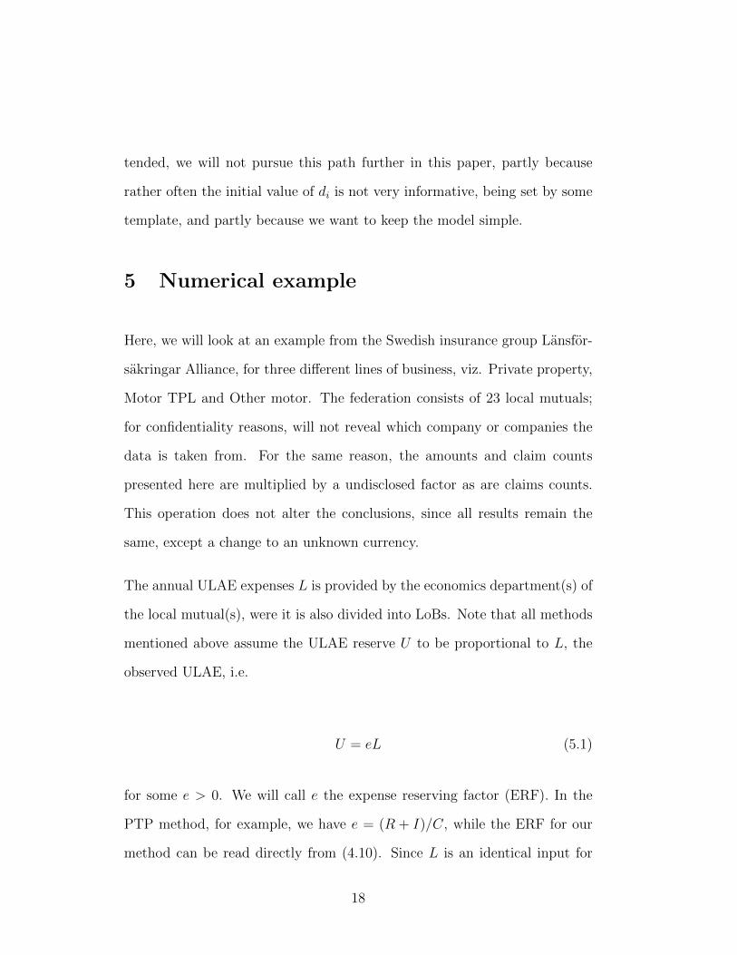
5 Numerical example
Here, we will look at an example from the Swedish insurance group Lansfor-
sakringar Alliance, for three different lines of business, viz. Private property,
Motor TPL and Other motor. The federation consists of 23 local mutuals;
for confidentiality reasons, will not reveal which company or companies the
data is taken from. For the same reason, the amounts and claim counts
presented here are multiplied by a undisclosed factor as are claims counts.
This operation does not alter the conclusions, since all results remain the
same, except a change to an unknown currency.
The annual ULAE expenses L is provided by the economics department(s) of
the local mutual(s), were it is also divided into LoBs. Note that all methods
mentioned above assume the ULAE reserve U to be proportional to L, the
observed ULAE, i.e.
U = eL (5.1)
for some e > 0. We will call e the expense reserving factor (ERF). In the
PTP method, for example, we have e = (R + I)/C, while the ERF for our
method can be read directly from (4.10). Since L is an identical input for
18
all the methods, the estimation problem for the actuary is how to choose the
method for computing the ERF.
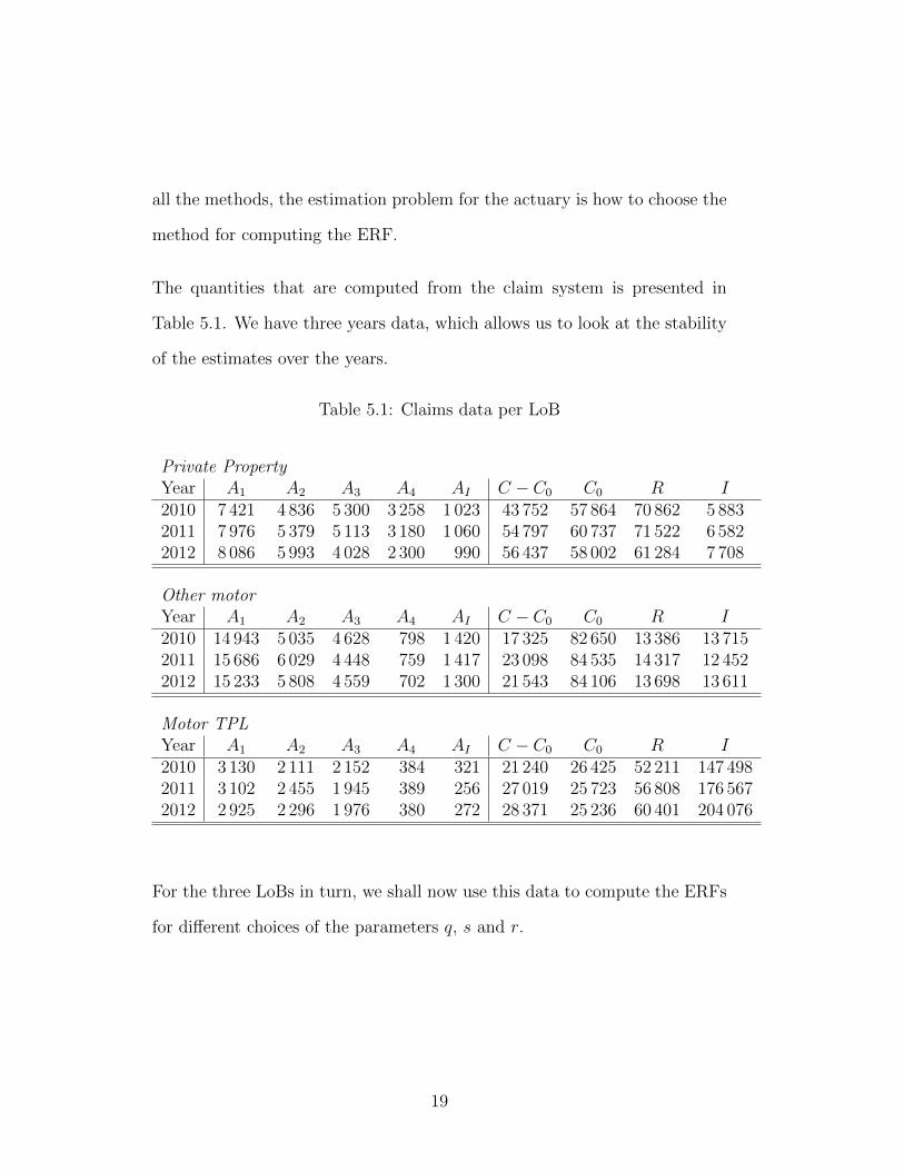
The quantities that are computed from the claim system is presented in
Table 5.1. We have three years data, which allows us to look at the stability
of the estimates over the years.
Table 5.1: Claims data per LoB
Private PropertyYear A1 A2 A3 A4 AI C − C0 C0 R I2010 7 421 4 836 5 300 3 258 1 023 43 752 57 864 70 862 5 8832011 7 976 5 379 5 113 3 180 1 060 54 797 60 737 71 522 6 5822012 8 086 5 993 4 028 2 300 990 56 437 58 002 61 284 7 708
Other motorYear A1 A2 A3 A4 AI C − C0 C0 R I2010 14 943 5 035 4 628 798 1 420 17 325 82 650 13 386 13 7152011 15 686 6 029 4 448 759 1 417 23 098 84 535 14 317 12 4522012 15 233 5 808 4 559 702 1 300 21 543 84 106 13 698 13 611
Motor TPLYear A1 A2 A3 A4 AI C − C0 C0 R I2010 3 130 2 111 2 152 384 321 21 240 26 425 52 211 147 4982011 3 102 2 455 1 945 389 256 27 019 25 723 56 808 176 5672012 2 925 2 296 1 976 380 272 28 371 25 236 60 401 204 076
For the three LoBs in turn, we shall now use this data to compute the ERFs
for different choices of the parameters q, s and r.
19

5.1 Private property
This LoB has a relatively short duration, so that most claims are finalized
within a few years. After five years, 99 % of the final amount is paid out and
the average payment duration is about one year. Claims in the reserve are
on the average larger than claims paid during the first year, implying that
r < 1 should be proper. As discussed above, we use r = 0.5 as the default
choice.
In Table 5.2 we have computed the ERFs resulting from the above data.
As a benchmark, we have added the ERF that would give the same ULAE
percentage of the reserve as the reported average among Swedish non-life
insurers. Note that this last factor, unlike the others, depends on L since it
is backed out from a percentage. It is included here only for comparison and
not as a candidate for estimation.
Table 5.2: ERFs for Private property
Model PTP Fixed Variable Default BenchmarkMix fixed/variable q = 0 q = 1 q = 0 q = 0.5Open/close split s = 0.5 s = 0.5First year loading r = 1 r = 0.5 r = 0.5ERF 2010 0.76 0.42 0.48 0.45 0.34ERF 2011 0.68 0.39 0.44 0.42 0.31ERF 2012 0.60 0.32 0.40 0.36 0.25
For PTP the ERF of 0.76 suggests that an amount equal to 76 % of the loss
adjustment cost for 2012 should be set off as ULAE reserve, and similar for
the other ERFs.
20

It is notable that this LoB is not very sensitive to the balance q between
the fixed and the variable cost models, so we can rather safely stay with
the default choice q = 0.5. The sensitivity to the other two parameters
is investigated in Table 5.3, where we compare the case with an opening
cost, but no closing cost, i.,e. s = 1, to our default s = 0.5. The other
extreme s = 0 would imply a fixed cost for closing and not for opening the
claim, which seems rather unrealistic and is therefore not included in our
comparison below. We also investigate the case with r = 1, i.e. equal ULAE
per paid amount, as compared to the default with r = 0.5, i.e. double cost per
currency unit for the first year’s payments, which includes a high frequency
of small claims. This gives us four combinations of s and r in Table 5.3.
Table 5.3: ERFs for Private property, sensitivity to s and r (q = 0.5)
Mixed model Simple Equal cost No closing DefaultOpen/close split s = 1 s = 0.5 s = 1 s = 0.5First year loading r = 1 r = 1 r = 0.5 r = 0.5ERF 2010 0.42 0.59 0.28 0.45ERF 2011 0.38 0.53 0.26 0.42ERF 2012 0.34 0.46 0.24 0.36
It is interesting that the simple model s = 1 and r = 1 gives very similar
results to the default model. Comparing to the presumably overestimating
PTP and the benchmark, which we guess might be a bit low, the other two
choices might be a bit high and low, respectively, and we decide to stay with
the default parameter values for Private property, i.e. q = 0.5, s = 0.5 and
r = 0.5.
21

5.2 Other motor
This LoB has very short duration, so that about 99 % of the claims are
finalized within the first two years. There are also few large claims. We do
not really expect claims that are finalized the first accounting year to be very
much smaller than the others and hence r = 1 seems a good candidate. For
completeness, we nevertheless present the same tables as for Private property
here.
Table 5.4: ERFs for Other motor
Model PTP Fixed Variable Default BenchmarkMix fixed/variable q = 0 q = 1 q = 0 q = 0.5Open/close split s = 0.5 s = 0.5First year loading r = 1 r = 0.5 r = 0.5ERF 2010 0.27 0.21 0.15 0.18 0.22ERF 2011 0.25 0.19 0.14 0.17 0.21ERF 2012 0.26 0.19 0.14 0.17 0.20
Table 5.5: ERFs for Other motor, sensitivity to s and r (q = 0.5)
Mixed model Simple Equal cost No closing DefaultOpen/close split s = 1 s = 0.5 s = 1 s = 0.5First year loading r = 1 r = 1 r = 0.5 r = 0.5ERF 2010 0.17 0.24 0.11 0.18ERF 2011 0.16 0.22 0.10 0.17ERF 2012 0.16 0.23 0.10 0.17
For this LoB, the choice of method does not seem that dramatic, and actually
the simple PTP might be considered, since we do not expect claims in the
reserve to be that much larger than the ones paid first year. Considering the
existence of zero claims makes us choose to include a fixed part anyway, but
22
as argued above take r = 1 in this case. The resulting ERF is close to both
PTP and the benchmark, which is a bit reinsuring, while the other choices
seem a bit low. Hence we use the model with q = 0.5, s = 0.5 and r = 1 for
Other motor.
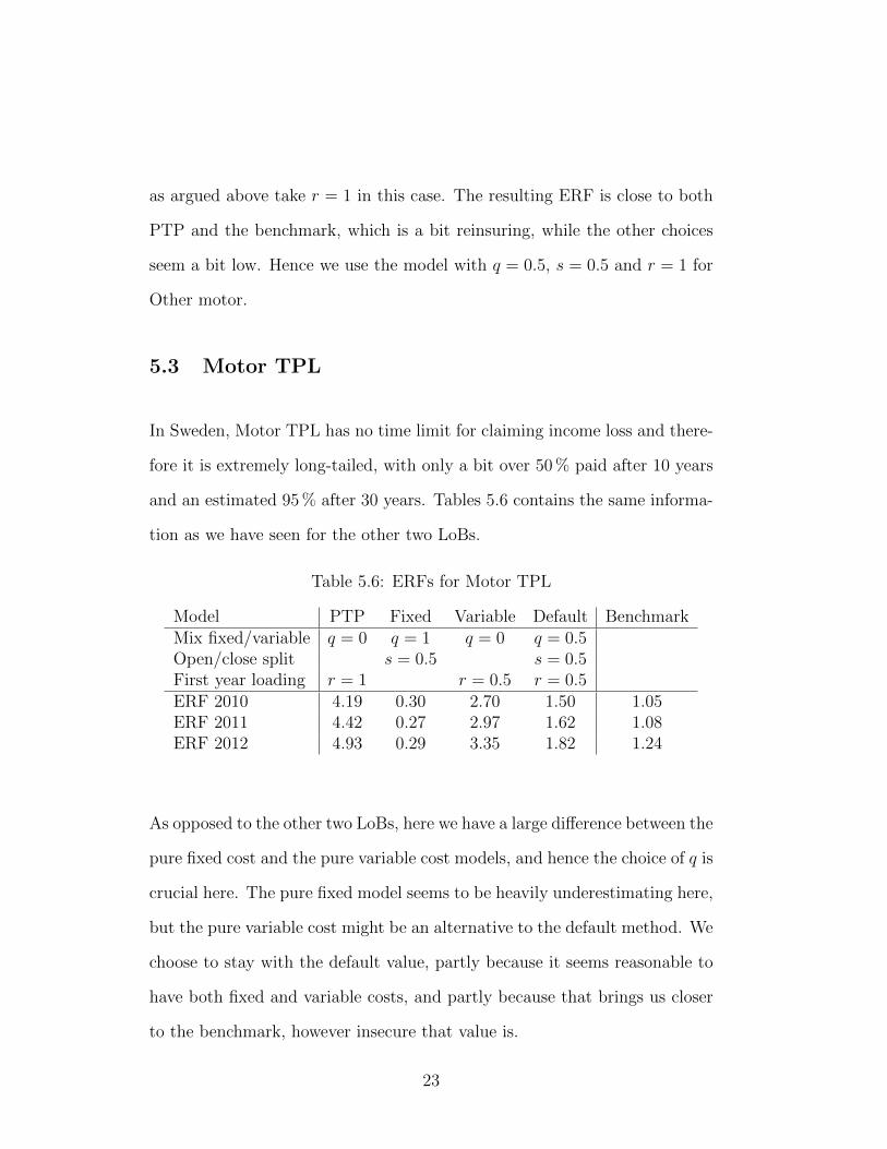
5.3 Motor TPL
In Sweden, Motor TPL has no time limit for claiming income loss and there-
fore it is extremely long-tailed, with only a bit over 50 % paid after 10 years
and an estimated 95 % after 30 years. Tables 5.6 contains the same informa-
tion as we have seen for the other two LoBs.
Table 5.6: ERFs for Motor TPL
Model PTP Fixed Variable Default BenchmarkMix fixed/variable q = 0 q = 1 q = 0 q = 0.5Open/close split s = 0.5 s = 0.5First year loading r = 1 r = 0.5 r = 0.5ERF 2010 4.19 0.30 2.70 1.50 1.05ERF 2011 4.42 0.27 2.97 1.62 1.08ERF 2012 4.93 0.29 3.35 1.82 1.24
As opposed to the other two LoBs, here we have a large difference between the
pure fixed cost and the pure variable cost models, and hence the choice of q is
crucial here. The pure fixed model seems to be heavily underestimating here,
but the pure variable cost might be an alternative to the default method. We
choose to stay with the default value, partly because it seems reasonable to
have both fixed and variable costs, and partly because that brings us closer
to the benchmark, however insecure that value is.
23
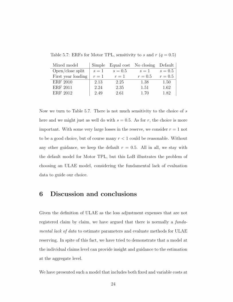
Table 5.7: ERFs for Motor TPL, sensitivity to s and r (q = 0.5)
Mixed model Simple Equal cost No closing DefaultOpen/close split s = 1 s = 0.5 s = 1 s = 0.5First year loading r = 1 r = 1 r = 0.5 r = 0.5ERF 2010 2.13 2.25 1.38 1.50ERF 2011 2.24 2.35 1.51 1.62ERF 2012 2.49 2.61 1.70 1.82
Now we turn to Table 5.7. There is not much sensitivity to the choice of s
here and we might just as well do with s = 0.5. As for r, the choice is more
important. With some very large losses in the reserve, we consider r = 1 not
to be a good choice, but of course many r < 1 could be reasonable. Without
any other guidance, we keep the default r = 0.5. All in all, we stay with
the default model for Motor TPL, but this LoB illustrates the problem of
choosing an ULAE model, considering the fundamental lack of evaluation
data to guide our choice.
6 Discussion and conclusions
Given the definition of ULAE as the loss adjustment expenses that are not
registered claim by claim, we have argued that there is normally a funda-
mental lack of data to estimate parameters and evaluate methods for ULAE
reserving. In spite of this fact, we have tried to demonstrate that a model at
the individual claims level can provide insight and guidance to the estimation
at the aggregate level.
We have presented such a model that includes both fixed and variable costs at
24

the claim level, leading to an estimator that only requires data at the aggre-
gate level. With the fundamental lack of data, some parameters in the model
have to be given arbitrary values, at the best based on expert judgement.
In our model this is the case for q, s and r. Under these circumstances, an
option would be that the supervisory authorities provided guidance or even
stipulated default values for these parameters; the latter is the case for the
“New york” model used in the Swiss Solvency Test.
In our numerical example, we tried to find a reasonable estimate of the ex-
pense reserving factor (ERF), which is to be multiplied by last years adjust-
ment expenses L in order to get the ULAE reserve in currency units. The
result is a smaller reserve than the PTP method would give – a desired result
since the PTP is generally known to be biased upwards. By construction,
our method with the default value q = 0.5 gives larger values than a pure
fixed cost model, which is also desired for similar reasons. It is also seen
to give larger values than the benchmark from Swedish non-life companies,
which is not very surprising for not that large local companies. Note that this
benchmark should be taken with a grain of salt, since we neither know the
methods used, nor the accuracy of the ULAE reserves in these companies.
There are of course other candidates as micro-level models than the exact
one used above, but to introduce a much more detailed model does not seem
motivated in this situation. This is even more so, since the result in the
end will depend heavily on the exact definition and computation of L, e.g.
in terms of overhead expenses, which can result in quite different values in
various companies.
25

Acknowledgements
Lansforsakringar Alliance is gratefully acknowledged for providing the oppor-
tunity to carry out this work. Special thanks to M. Sc. Svante Barck-Holst
for gathering data and carrying out the numerical computations.
26

References
Buchwalder, M., Merz, M., Buhlmann, H., & Wutrich, M.V. (2006). Estima-
tion of Unallocated Loss Adjustment Expenses. Schweiz. Aktuariev. Mitt.
2006/1, 43-53.
Conger, R.F. & Nolibos, A. (2003). Estimating ULAE Liabilities: Redis-
covering and Expanding Kittel’s Approach. CAS Forum Fall 2003, 94-139.
Available at www.casact.com
Institute of Actuaries (1997). Claims Reserving Manual. The faculty and
Institute of Acturies. Available at www.actuaries.org.uk
Johnson, W. (1989): Determination of outstanding liabilities for unallocated
loss adjustment expenses. PCAS LXXVII, 1989, 111-125. Available at
www.casact.com
Kittel, J. (1981): Unallocated loss adjustment expense reserves in an inflatory
economic environment. CAS Discussion Paper Program, 311-331. Available
at www.casact.com
Mango, D.F. & Allen, C.A. (1999). Two alternative methods for estimating
the unallocated loss adjustment expense reserve. CAS Forum Fall 1999.
Available at www.casact.com
Schnieper (1991). Separating true IBNR and IBNER claims. ASTIN Bulletin
21, 111-127.
27

Spalla, J. S. (2001): Using claim department work measurement systems to
determine claims adjustment expense reserves. PCAS LXXXVIII, 64-115.
Available at www.casact.com
28
Recommended