Tutorial Nine
Parallel Processing
4th edition, Jan. 2018
This offering is not approved or endorsed by ESI® Group, ESI-OpenCFD® or the OpenFOAM®
Foundation, the producer of the OpenFOAM® software and owner of the OpenFOAM® trademark.
OpenFOAM
® Basic Training
Tutorial Nine
Editorial board:
Bahram Haddadi
Christian Jordan
Michael Harasek
Compatibility:
OpenFOAM® 5.0
OpenFOAM® v1712
Cover picture from:
Bahram Haddadi
Contributors:
Bahram Haddadi
Clemens Gößnitzer
Jozsef Nagy
Vikram Natarajan
Sylvia Zibuschka
Yitong Chen
Attribution-NonCommercial-ShareAlike 3.0 Unported (CC BY-NC-SA 3.0)
This is a human-readable summary of the Legal Code (the full license). Disclaimer You are free:
- to Share — to copy, distribute and transmit the work - to Remix — to adapt the work
Under the following conditions: - Attribution — You must attribute the work in the manner specified by the author or
licensor (but not in any way that suggests that they endorse you or your use of the work).
- Noncommercial — You may not use this work for commercial purposes. - Share Alike — If you alter, transform, or build upon this work, you may distribute the
resulting work only under the same or similar license to this one. With the understanding that:
- Waiver — Any of the above conditions can be waived if you get permission from the copyright holder.
- Public Domain — Where the work or any of its elements is in the public domain under applicable law, that status is in no way affected by the license.
- Other Rights — In no way are any of the following rights affected by the license: - Your fair dealing or fair use rights, or other applicable copyright exceptions and
limitations; - The author's moral rights; - Rights other persons may have either in the work itself or in how the work is used,
such as publicity or privacy rights. - Notice — For any reuse or distribution, you must make clear to others the license
terms of this work. The best way to do this is with a link to this web page.
For more tutorials visit: www.cfd.at
OpenFOAM
® Basic Training
Tutorial Nine
Background
In this tutorial we will analyze compressible fluid flow in OpenFOAM®. Parallel
processing is utilized to speed up the simulation. In this introduction part, theory
behind compressible flow, solvers for compressible flow and parallel computing will
be explained in detail.
1. Introduction to compressible flow
So far we have only considered incompressible fluid flows, however in many
situations; there may be a significant change in the density. One example of
compressible flow is the flow through a diverging-converging nozzle. Compressibility
becomes dominant in flows when the Mach number is greater than about 0.3. The
Mach number is defined as follows:
When a fluid flow is compressible, temperature and pressure are affected strongly by
variations in density. It is therefore important to take into account the linkage between
pressure, temperature and density in compressible flow, usually by applying an
equation of state from thermodynamics (e.g. the ideal gas equation).
2. Compressible flow solvers
There are two general types of solution schemes for compressible flow: pressure-
based and density-based.
2.1. Pressure-based solvers
This type of solver was historically derived from the solution approach used on
incompressible flows. They solve for the primitive variables. The discretized
momentum and energy equations are used to update velocities and energy. The
pressure is obtained by applying a pressure-correction algorithm on the continuity and
momentum equations. Density is then calculated from the equation of state.
2.2. Density-based solvers
Density-based solvers are suitable for solving the conserved variables. Similar to
pressure-based solvers, the conversed velocity and energy terms are updated from the
discretized momentum and energy equations. We can then solve for density from the
continuity equation, afterwards we use the equation of state to update the pressure.
In general, density based solvers are more suitable for high speed compressible flows
with shocks. This is because density based solvers solve for conserved quantities
across the shock, so the discontinuities will not affect the results.
3. Parallel computing
Imagine if we need to tackle a complex CFD problem that involves complex
geometry, multiphase flow, turbulence and reaction, how do we adopt a methodical
computational approach to save time and cost? This is when parallel computing
OpenFOAM
® Basic Training
Tutorial Nine
comes in. Parallel computing is defined as the simultaneous use of more than one
processor to execute a program. The geometry of the domain will be partitioned into
sub-domains, with each sub-domain assigned to a single processor. Furthermore data
and computational tasks will be partitioned and divided amongst the processors. This
step is known as domain decomposition.
Parallel computing can be carried out in two ways. One is done on a single computer
with multiple internal processors, known as a Shared Memory Multiprocessor. The
other way is achieved through a series of computers interconnected by a network,
known as a Distributed Memory Multicomputer.
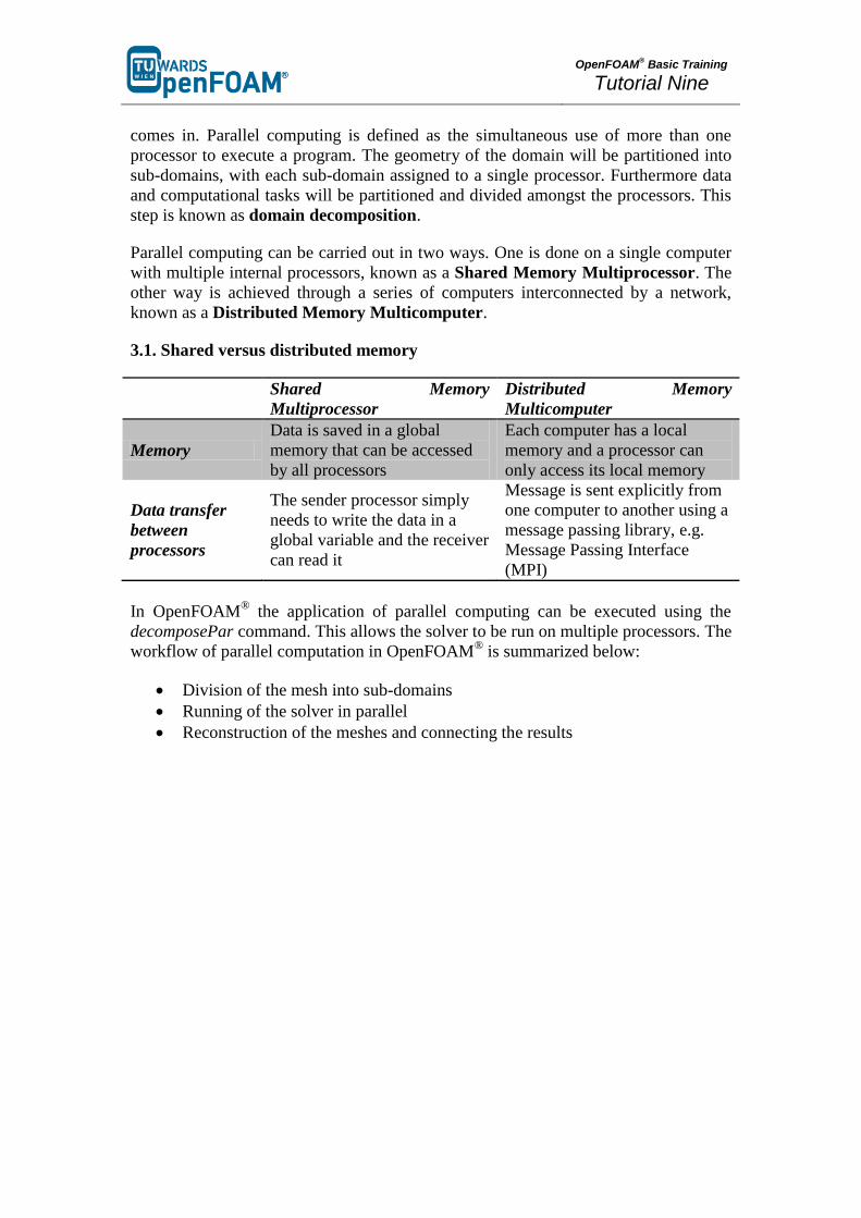
3.1. Shared versus distributed memory
Shared Memory
Multiprocessor
Distributed Memory
Multicomputer
Memory
Data is saved in a global
memory that can be accessed
by all processors
Each computer has a local
memory and a processor can
only access its local memory
Data transfer
between
processors
The sender processor simply
needs to write the data in a
global variable and the receiver
can read it
Message is sent explicitly from
one computer to another using a
message passing library, e.g.
Message Passing Interface
(MPI)
In OpenFOAM® the application of parallel computing can be executed using the
decomposePar command. This allows the solver to be run on multiple processors. The
workflow of parallel computation in OpenFOAM®
is summarized below:
Division of the mesh into sub-domains
Running of the solver in parallel
Reconstruction of the meshes and connecting the results
OpenFOAM
® Basic Training
Tutorial Nine
compressibleInterFoam – depthCharge3D
Simulation
Use the compressibleInterFoam solver, simulate the example case for 0.5 s.
Objectives
Understanding the difference between incompressible and compressible
solvers
Understanding parallel processing and different discretization methods
Data processing
Investigate the results in ParaView.
OpenFOAM
® Basic Training
Tutorial Nine
1. Pre-processing
1.1. Copy tutorial
Copy the tutorial from following directory to your working directory:
$FOAM_TUTORIALS/multiphase/compressibleInterFoam/laminar/depth
Charge3D
1.2. 0 directory
Create a 0 directory and copy all the files from the 0.orig directory to the 0 directory.
1.3. constant directory
Phases and common physical properties of the two phases are set in the
thermophysicalProperties file. Individual phase properties are set in
thermophysicalProperties.phase files, e.g. thermophysicalProperties.air.
// * * * * * * * * * * * * * * * * * * * * * * * * * * * * * * * * * * * * * * *
* * * * * *//
phases (water air);
pMin 10000;
sigma 0.07;
// * * * * * * * * * * * * * * * * * * * * * * * * * * * * * * * * * * * * * * *
* * * * * *//
1.4. system directory
The decomposeParDict file includes the parallel settings, such as the number of
domains (partitions) and also how the domain is going to be divided into these
subdomains for parallel processing.
// * * * * * * * * * * * * * * * * * * * * * * * * * * * * * * * * * * * * * * *
* * * * * *//
numberOfSubdomains 4;
method hierarchical;
simpleCoeffs
{
n ( 1 4 1 );
delta 0.001;
}
hierarchicalCoeffs
{
n ( 1 4 1 );
delta 0.001;
order xyz;
}
manualCoeffs
{
dataFile "";
}
distributed no;
roots ( );
// * * * * * * * * * * * * * * * * * * * * * * * * * * * * * * * * * * * * * * *
* * * * * *//
OpenFOAM
® Basic Training
Tutorial Nine
OpenFOAM® v1712: In this file just the coefficients for hierarchical method are
listed!
numberOfSubdomains should be equal to the number of cores used. method
should show the method to be used. In the above example, the case is simulated with
the hierarchical method and 4 processors.
If the simple method is being used, the parameter n must be changed accordingly.
The three numbers (1 4 1) indicate the number of pieces the mesh is split into in
the x, y and z directions, respectively. Their multiplication result should be equal to
numberOfSubdomains.
If the hierarchical method is being used, these parameters and also the order in
which the mesh should be split up in each direction should be provided.
If the scotch method is being used, then no user-supplied parameters are necessary
except for the number of subdomains.
There is also a parameter delta, known as the cell skew factor. This factor is set to a
default value of 0.001, and measures to what extent skewed cells should be
accounted for.
Note: In order to check the quality of the mesh, the checkMesh tool can be used (run it
from main case directory). If the message “Mesh OK” is displayed – the mesh is fine
and no corrections need to be done.
If the mesh fails in one or more tests, try to recreate or refine the mesh for a better
mesh quality (less non-orthogonally and skewness). If the error exists after correcting
the mesh then a possible course of action is to increase the delta parameter (for
example: to 0.01) and then rerun the blockMesh and checkMesh tools.
If non-orthogonal cells exist in a mesh, another option is using non-orthogonal
corrections in the fvSolution file in the algorithm sub-dictionary (e.g. PIMPLE or
PISO). Usually using 1 or 2 as nNonOrthogonalCorrectors is enough.
2. Running simulation
>blockMesh
>setFields
For running the simulation in parallel mode the computing domain needs to be
divided into subdomains and a core should be assigned to each subdomain. This is
done by following command:
>decomposePar
This decomposes the mesh according to the supplied instructions. One possible source
of error is the product of the parameters in n does not match up to the number of the
subdomains. This appears for the simple and hierarchical methods.
OpenFOAM
® Basic Training
Tutorial Nine
After executing this command four new directories will be made in the simulation
directory (processor0, processor1, processor2 processor3), and each subdomain
calculation will be saved in the respective processor directory.
Note: When the domain is divided to subdomains in parallel processing new
boundaries are defined. The data should be exchanged with the neighbor boundary,
which it is connected to in the main domain.
>mpirun -np <No of cores> solver –parallel > log
<No of cores> is the number of cores being used. solver is the solver for this
simulation. For example, if 4 cores are desired, and the solver is
compressibleInterFoam following command is used:
>mpirun -np 4 compressibleInterFoam -parallel > log
> log is the filename for saving the simulation status data, instead of printing them
to the screen. For checking the last information which is written to this file the
following command can be used during the simulation running:
>tail –f log
Note: Before running any simulation, it is important to run the top command (type the
„top‟ command in the terminal), to check the number of cores currently used on the
machine. Check the load average. This is on the first line and shows the average
number of cores being used. There are three numbers displayed, showing the load
averages across three different time scales (one, five and 15 minute respectively).
Add the number of cores you plan to use to this number – and you will get the
expected load average during your simulation. This number should be less than the
total number of cores in the machine – or the simulation will be slowed or the
machine will crash (if you run out of memory). If you are running on a multi user
server it is recommended to leave at least a few cores free, to allow for any
fluctuations in the machine load.
Note: top command execution can be interrupted by typing q (or ctrl+c)
The simulation can take several hours, depending on the size of the mesh and time
step size.
3. Post-processing
For exporting data for post processing, at first all the processors data should be put
together and a single combined directory for each time step was created. By executing
the following command all the cores data will be combined and new directories for
each time step will be created in the simulation main directory:
>reconstructPar
Convert the data to ParaView format:
>foamToVTK
OpenFOAM
® Basic Training
Tutorial Nine
Note: To do the reconstruction or foamToVTK conversion from a start time until an
end time the following flags can be used:
>reconstructPar –time [start time name, e.g. 016]:[end time
name, e.g. 020]
>foamToVTK –time [start time name, e.g. 016]:[end time name,
e.g. 020]
Using above commands without entering end time will do the reconstruction or
conversion from start time to the end of available data:
>reconstructPar –time [start time name, e.g. 016]:
>foamToVTK –time [start time name, e.g. 016]:
For reconstructing or converting only one time step the commands should be used
without end time and “:”:
>reconstructPar –time [start time name, e.g. 016]
>foamToVTK –time [start time name, e.g. 016]
OpenFOAM
® Basic Training
Tutorial Nine
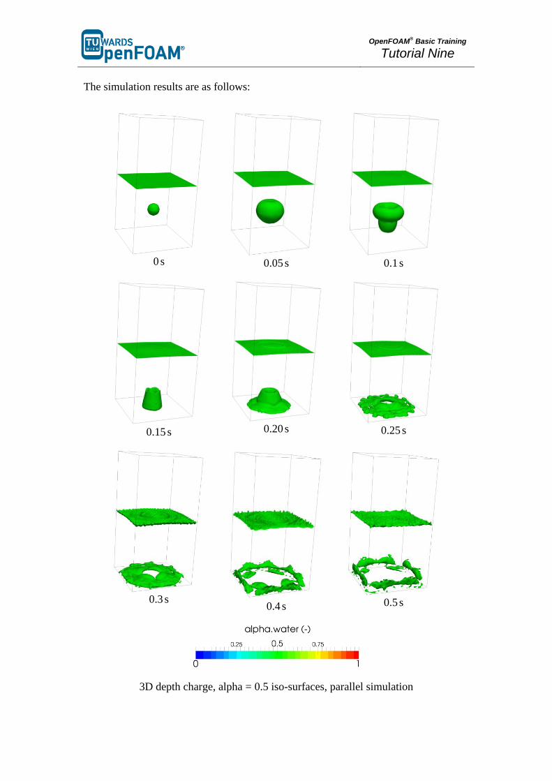
The simulation results are as follows:
0 s
0.05 s
0.1 s
0.15 s
0.20 s
0.25 s
0.3 s
0.4 s
0.5 s
3D depth charge, alpha = 0.5 iso-surfaces, parallel simulation
OpenFOAM
® Basic Training
Tutorial Nine
4. Manual method
4.1 Case set-up and running simulation
The manual method for decomposition is slightly different from the other three. In
order to use it:
After running the blockMesh and setFields utilities, set the decomposeParDict file as
any other simulation. For decomposition method, choose either simple, hierarchical or
scotch. Set the number of cores to the same number which is going to be used for
manual.
>decomposePar –cellDist
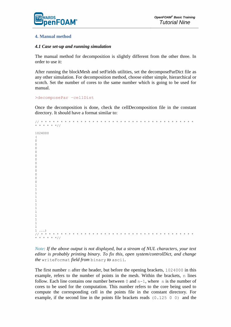
Once the decomposition is done, check the cellDecomposition file in the constant
directory. It should have a format similar to:
// * * * * * * * * * * * * * * * * * * * * * * * * * * * * * * * * * * * * * * *
* * * * * *//
1024000
(
0
0
0
0
0
0
0
0
0
0
0
0
1
1
1
1
1
1
1
1
1
1
1
1
1 ...)
// * * * * * * * * * * * * * * * * * * * * * * * * * * * * * * * * * * * * * * *
* * * * * *//
Note: If the above output is not displayed, but a stream of NUL characters, your text
editor is probably printing binary. To fix this, open system/controlDict, and change
the writeFormat field from binary to ascii.
The first number n after the header, but before the opening brackets, 1024000 in this
example, refers to the number of points in the mesh. Within the brackets, n lines
follow. Each line contains one number between 0 and n-1, where n is the number of
cores to be used for the computation. This number refers to the core being used to
compute the corresponding cell in the points file in the constant directory. For
example, if the second line in the points file brackets reads (0.125 0 0) and the
OpenFOAM
® Basic Training
Tutorial Nine
second line in the cellDecomposition directoy reads 0, this means that the cell
(0.125 0 0) will be processed by processor 0.
This cellDecomposition file can now be edited. Although this can be done manually,
it is probably not feasible for any sufficiently large mesh. The process must thus be
automated by writing a script to populate the cellDecomposition file according to the
desired processor breakdown.
When the new file is ready, save it under a different name:
>cp cellDecomposition manFile
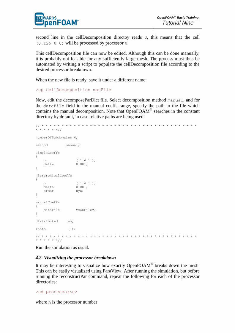
Now, edit the decomposeParDict file. Select decomposition method manual, and for
the dataFile field in the manual coeffs range, specify the path to the file which
contains the manual decomposition. Note that OpenFOAM® searches in the constant
directory by default, in case relative paths are being used:
// * * * * * * * * * * * * * * * * * * * * * * * * * * * * * * * * * * * * * * *
* * * * * *//
numberOfSubdomains 4;
method manual;
simpleCoeffs
{
n ( 1 4 1 );
delta 0.001;
}
hierarchicalCoeffs
{
n ( 1 4 1 );
delta 0.001;
order xyz;
}
manualCoeffs
{
dataFile "manFile";
}
distributed no;
roots ( );
// * * * * * * * * * * * * * * * * * * * * * * * * * * * * * * * * * * * * * * *
* * * * * *//
Run the simulation as usual.
4.2. Visualizing the processor breakdown
It may be interesting to visualize how exactly OpenFOAM® breaks down the mesh.
This can be easily visualized using ParaView. After running the simulation, but before
running the reconstructPar command, repeat the following for each of the processor
directories:
>cd processor<n>
where n is the processor number
OpenFOAM
® Basic Training
Tutorial Nine
>foamToVTK
convert the individual processor files to VTK, next, open ParaView:
>paraview &
For each of the processor directories, perform the following steps:
- Open the VTK files in the relevant processor directory
- Double click them to open them and click on “Apply”
- The part of the mesh decomposed by that core will appear, in grey.
- Change the color in the drop-down menus in the toolbar. This is to ensure that each
individual part can be easily seen.
Once this is done for all processors, the entire mesh will appear. However, the
processor regions can now easily be seen in a different color.
In order to save this, there are two options. The first option is to take a screenshot:
File > Save a screenshot
The second option is to save the settings and modifications as a ParaView state file.
File > Save State
The current settings and modifications can then be easily recovered by:
File > Load State
Saving the state allows changes to be made afterwards. Saving a screenshot keeps
only a picture, while losing the ability to make changes after exiting ParaView. Doing
both is recommended.
Recommended