UNCLASSIFIED
Trim Calculation Methods for a Dynamical Model of the REMUS 100 Autonomous Underwater Vehicle
Raewyn Hall and Stuart Anstee
Maritime Operations Division Defence Science and Technology Organisation
DSTO-TR-2576
ABSTRACT The calculations given in this work demonstrate that the trimmed state for a dynamical model of the REMUS 100 autonomous underwater vehicle is readily found using a numerical zero-finding procedure based on Newton-Raphson iteration. This work also presents approximate analytical expressions for the trimmed state that can be used as a starting point for the numerical procedure. The procedure should be applicable to a range of hydrodynamic parameters corresponding to other configurations of the REMUS 100 vehicle and to similar vehicles from other vendors.
RELEASE LIMITATION
Approved for public release
UNCLASSIFIED
UNCLASSIFIED
Published by Maritime Operations Division DSTO Defence Science and Technology Organisation PO Box 1500 Edinburgh South Australia 5111 Australia Telephone: (08) 7389 5555 Fax: (08) 7389 6567 © Commonwealth of Australia 2011 AR-015-046 August 2011 APPROVED FOR PUBLIC RELEASE
UNCLASSIFIED
UNCLASSIFIED
UNCLASSIFIED
Trim Calculation Methods for a Dynamical Model of the REMUS 100 Autonomous Underwater Vehicle
Executive Summary Survey-class autonomous underwater vehicles (AUVs) are used to investigate the seabed and the water column with high resolution and navigational accuracy. The Royal Australian Navy (RAN) is in the process of acquiring AUVs for use in mine countermeasures, Rapid Environmental Assessment and Advance Force operations. AUVs are potentially major components of acquisition projects SEA 1778 Phase 1 Deployable MCM – Organic Mine Countermeasures and JP 1770 Phase 1 Rapid Environmental Assessment. They may also be components of off-board mission systems that will be acquired as part of future projects SEA 1180 Phase 1 - Patrol Boat, Mine Hunter Coastal and Hydrographic Ship Replacement Project and SEA 1000, Future Submarine. The DSTO acquired two commercial AUVs in 2007, in collaboration with the Directorate General of Maritime Development and the RAN. One of the AUVs was a REMUS 100, manufactured by Kongsberg Hydroid Incorporated of the USA. Many navies have one or more REMUS 100 vehicles in their inventory and the number of REMUS 100s that has been produced is of the same order as the number of all other commercial AUVs in existence, combined. Although the DSTO vehicle has been extensively tested, its high value precludes testing in waters where currents are strong, or shallow and wave-driven, since the vehicle might be damaged, lost or destroyed. However, operating areas in which such conditions occur are potentially of high military value and there is considerable interest in being able to predict the limiting conditions for use of the vehicle. As a consequence, the DSTO has begun to investigate techniques by which the dynamics of the vehicle may be simulated with appropriate fidelity, using so-called ‘low-level’ simulation models based on estimates of the governing equations of motion for the vehicle. Accurate low-level simulations of vehicle behaviour rely on well-behaved numerical implementations. One component of such implementations is the ‘trim’ state of the model, which, for a given speed, is the combination of vehicle orientation and control settings in which the unperturbed vehicle will maintain straight-line, level flight in a state of dynamic equilibrium. The trim state is used to analyse the stability of the numerical model – its response to perturbations away from the trim state – and to initialise simulations. This work describes a robust, parametric process to estimate the trim state of a dynamical model of the REMUS 100 AUV based on equations of motion originally developed by Prestero [1] and extended by Sgarioto [2]. The method is based on direct solution of the governing equations of motion, using an iterative Newton-Raphson zero-finding algorithm. The algorithm is initialised using second-order analytical approximations to the
UNCLASSIFIED
UNCLASSIFIED
Prestero-Sgarioto equations of motion. The relative accuracy of the analytical expressions is better than 1% at speeds near the cruising speed of the vehicle, but decreases by 1 to 2 orders of magnitude at lower speeds. Other methods of initialisation were also investigated and a reduced set of analytical expressions was found to be effective as a starting point for the iterative calculation. A parametric investigation showed that the iterative algorithm was convergent for speeds from 1 knot to at least 6 knots; in comparison, the physical vehicle operates within a range of speeds between 2 knots and 5 knots. The variation of the trimmed state conformed to expectations over the latter range. Unexpected behaviour was seen at lower speeds, but this did not originate from a failure of the trim calculation. In summary, this work has resulted in a procedure for finding the trimmed state of the Prestero AUV dynamics model using a straightforward numerical method with a parametric initialisation procedure. With appropriate parameters, the method should be applicable to variations of the REMUS vehicle; for example, extended versions, and to other REMUS-like vehicles. References cited in this section:
1. Prestero, T. “Verification of a Six-Degree-of-Freedom Simulation Model for the REMUS Autonomous Underwater Vehicle”, MSc/ME Thesis, Massachusetts Institute of Technology, Sept. 2001.
2. Sgarioto, D. “Steady State Trim and Open Loop Stability Analysis for the REMUS Autonomous Underwater Vehicle”, Defence Technology Agency, New Zealand Defence Force, DTA Report 254, March 2008.
UNCLASSIFIED
UNCLASSIFIED
Authors
Raewyn Hall Maritime Operations Division Raewyn graduated from Sydney University in 2005 with honours in Aeronautical (Space) Engineering and a Bachelor of Science. Her engineering honours thesis focussed on aircraft flight dynamics, guidance and model predictive control. She joined the Maritime Operations Division in 2006 doing operations analysis and modelling in a variety of areas such as amphibious operations and anti-submarine warfare. She currently splits her time between the Maritime Concepts and Capabilities Group and modelling AUV dynamics for the Littoral Unmanned Systems Group.
____________________ ________________________________________________
Stuart Anstee Maritime Operations Division Stuart Anstee is a member of the Littoral Unmanned Systems Group, which investigates the application of unmanned vehicles to mine warfare and hydrography. In his career at DSTO, he has worked on the design, modelling and assessment of high-frequency sonars, analysis tools for sonar imagery and operations research. His current interests include assessment of autonomous vehicle systems, the hydrodynamics and control of underwater vehicles, autonomous mission planning and investigation of sensors for mine warfare and hydrography.
____________________ ________________________________________________

UNCLASSIFIED
UNCLASSIFIED
This page is intentionally blank
UNCLASSIFIED
Contents
1. INTRODUCTION............................................................................................................... 1
2. THE REMUS 100 MODEL................................................................................................. 1 2.1 The REMUS 100 Vehicle.......................................................................................... 1 2.2 Simulation Model ..................................................................................................... 2
2.2.1 Notation .................................................................................................... 2 2.2.2 Mathematical Representation ................................................................ 4
2.3 Coordinate Transformations................................................................................... 4 2.3.1 Earth and Body Reference Frames ........................................................ 4 2.3.2 Body and Stability Reference Frames ................................................... 5
2.4 Equations of Motion................................................................................................. 6 2.5 External Forces and Moments................................................................................. 7
3. ESTIMATION OF TRIM ................................................................................................... 8 3.1 Definition of Trim .................................................................................................... 8 3.2 Trim Variables........................................................................................................... 8 3.3 Decision Variables.................................................................................................... 9 3.4 Trim Estimation by Numerical Iteration.............................................................. 9
3.4.1 Newton-Raphson Iteration..................................................................... 9 3.4.2 Implementation...................................................................................... 10 3.4.3 Performance of the Newton-Raphson Iteration ................................ 10 3.4.4 Convergence Sensitivity ....................................................................... 11
3.5 Estimation of the Starting Point for the Iteration ............................................. 12 3.5.1 Empirical and Analytical Starting Points........................................... 12 3.5.2 Simplified Analytical Starting Point ................................................... 13 3.5.3 Results and Discussion ......................................................................... 13
4. PARAMETRIC STUDY.................................................................................................... 14 4.1 Vehicle Orientation Angles .................................................................................. 14 4.2 Propulsion Variables.............................................................................................. 15 4.3 Control Inputs ......................................................................................................... 16
5. CONCLUSION .................................................................................................................. 17
6. REFERENCES .................................................................................................................... 18
APPENDIX A: REMUS 100 MODEL PARAMETERS .................................................. 19 A.1. Mathematical Symbols.................................................................. 19 A.2. Case Study Parameters .................................................................. 20
APPENDIX B: ALGORITHM IMPLEMENTATION ................................................... 23
UNCLASSIFIED
UNCLASSIFIED
B.1. Interface Function .......................................................................... 23 B.2. Iteration Algorithm........................................................................ 24
B.2.1 Jacobian matrix calculation............................................. 24 B.3. Trim function MATLAB script .................................................... 26
B.3.1 Main Trim Function ‘trim.m’ .......................................... 26 B.3.2 Equations of Motion Function ‘eom.m’.......................... 28 B.3.3 Hydrodynamics Coefficients script file ‘coeffs.m’ ........ 31
APPENDIX C: ANALYTICAL TRIM ESTIMATION USING FORCE BALANCE CONDITIONS .......................................................................................... 34 C.1. Senses of Motion ............................................................................ 34 C.2. Approximation to Nearly Level Motion .................................... 35 C.3. Derivation of Analytical Approximations................................. 37
C.3.1 Propulsion Subsystem..................................................... 37 C.3.2 Manoeuvre Subsystem.................................................... 37
C.4. Comparison of Numerical and Analytical Trim Estimates .... 38
APPENDIX D: CONVERGENCE SENSITIVITY ANALYSIS .................................... 43
UNCLASSIFIED

UNCLASSIFIED
GLOSSARY AUV Autonomous Underwater Vehicle
GPS Global Positioning System
INS Inertial Navigation System
LBL Acoustic Long Baseline navigation system
RAN Royal Australian Navy
UNCLASSIFIED

UNCLASSIFIED
UNCLASSIFIED
This page is intentionally blank
UNCLASSIFIED DSTO-TR-2676
1. Introduction
Survey-class autonomous underwater vehicles (AUVs) are used to investigate the seabed and the water column with high resolution and navigational accuracy. The Royal Australian Navy (RAN) is in the process of acquiring AUVs for use in mine countermeasures, Rapid Environmental Assessment (REA) and Advance Force operations. AUVs are potentially major components of acquisition projects SEA 1778 Phase 1 Deployable MCM – Organic Mine Countermeasures and JP 1770 Phase 1 Rapid Environmental Assessment. They may also be components of off-board mission systems that will be acquired as part of future project SEA 1180 Phase 1 - Patrol Boat, Mine Hunter Coastal and Hydrographic Ship Replacement Project and SEA 1000, Future Submarine. The DSTO acquired two commercial AUVs in 2007, in collaboration with the Directorate General of Maritime Development and the RAN. One of the AUVs was a REMUS 100, manufactured by Kongsberg Hydroid Incorporated of the USA. Although this vehicle has been extensively tested, its high value precludes its inclusion in trials where currents are excessively strong or waters are shallow and wave-driven, since damage or loss of the vehicle might result. As a consequence, the DSTO has begun to investigate techniques by which the dynamics of the vehicle might be simulated in extreme environments. High-fidelity simulations of vehicle behaviour rely on well-behaved numerical models. A starting point for such models is the ‘trim’ state of the vehicle, corresponding to the control state in which it will maintain straight-line, level flight in a state of dynamic equilibrium. This report describes analytical and numerical methods that may be used to trim a non-linear, six degree-of-freedom simulation model describing the dynamics of a REMUS 100 AUV. The convergence properties of the trim calculation and the nature of the trim state are also examined as a function of the model parameters.
2. The REMUS 100 Model
2.1 The REMUS 100 Vehicle
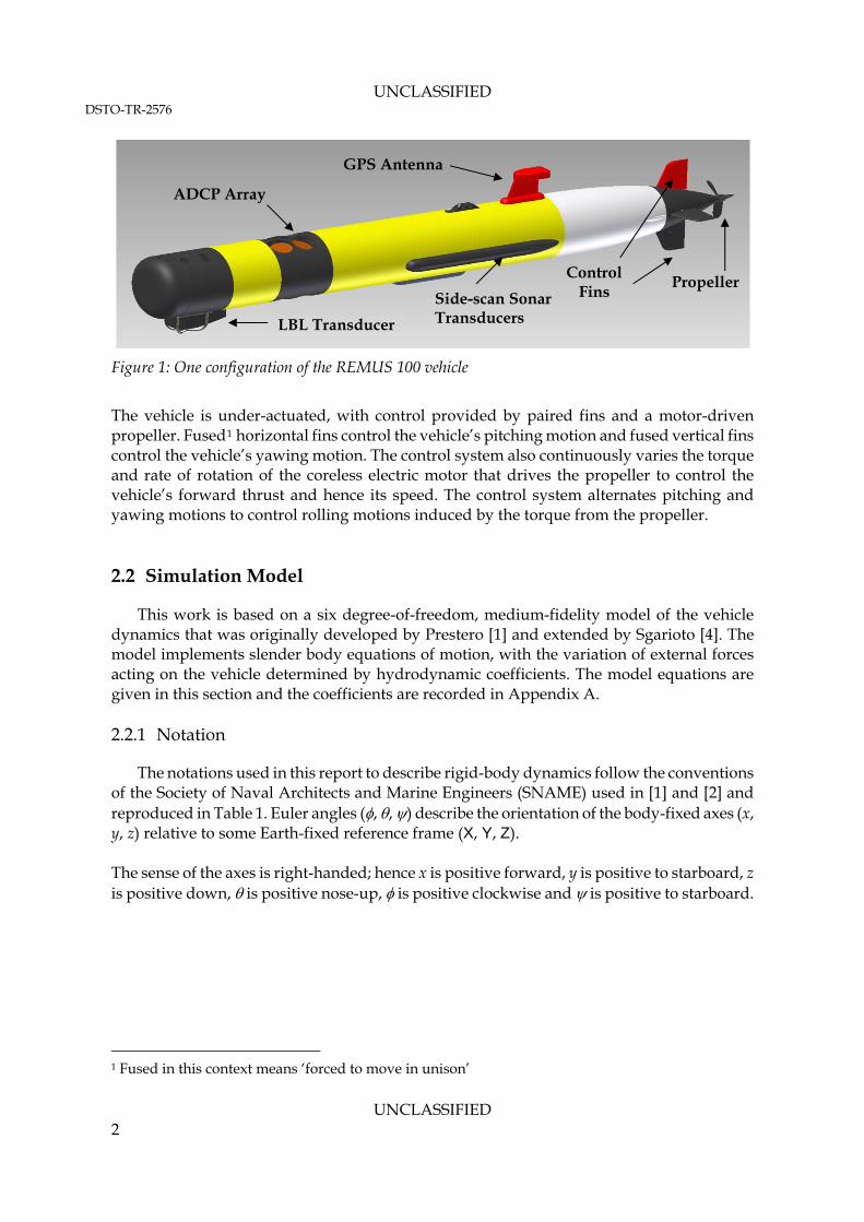
The REMUS 100 is a slender, torpedo-shaped vehicle, as shown in Figure 1. It is approximately 1.6 to 1.72 m long, has a diameter of 19 cm and weighs 36 to 40 kg in air, depending on configuration. It is designed to execute pre-programmed missions in order to collect sonar imagery of the seafloor, operating at ground speeds from 2.5 to 4.5 knots. The main payload sensor is side-scan sonar, which is typically used to gather imagery of the sea floor. The vehicle has a suite of other sensors, including a pressure sensor, a conductivity sensor, a thermometer, an acoustic long-baseline (LBL) transceiver, upward and downward-pointing acoustic Doppler current profilers and a GPS receiver, all of which may optionally be used to aid an inertial navigation system (INS).
UNCLASSIFIED 1
UNCLASSIFIED DSTO-TR-2576
GPS Antenna
Figure 1: One configuration of the REMUS 100 vehicle
The vehicle is under-actuated, with control provided by paired fins and a motor-driven propeller. Fused1 horizontal fins control the vehicle’s pitching motion and fused vertical fins control the vehicle’s yawing motion. The control system also continuously varies the torque and rate of rotation of the coreless electric motor that drives the propeller to control the vehicle’s forward thrust and hence its speed. The control system alternates pitching and yawing motions to control rolling motions induced by the torque from the propeller. 2.2 Simulation Model
This work is based on a six degree-of-freedom, medium-fidelity model of the vehicle dynamics that was originally developed by Prestero [1] and extended by Sgarioto [4]. The model implements slender body equations of motion, with the variation of external forces acting on the vehicle determined by hydrodynamic coefficients. The model equations are given in this section and the coefficients are recorded in Appendix A. 2.2.1 Notation
The notations used in this report to describe rigid-body dynamics follow the conventions of the Society of Naval Architects and Marine Engineers (SNAME) used in [1] and [2] and reproduced in Table 1. Euler angles (, , ) describe the orientation of the body-fixed axes (x, y, z) relative to some Earth-fixed reference frame (X, Y, Z). The sense of the axes is right-handed; hence x is positive forward, y is positive to starboard, z is positive down, is positive nose-up, is positive clockwise and is positive to starboard.
1 Fused in this context means ‘forced to move in unison’
Propeller
ADCP Array
Control Fins Side-scan Sonar
Transducers LBL Transducer
UNCLASSIFIED 2
UNCLASSIFIED DSTO-TR-2676
Table 1: Symbols used to describe rigid-body dynamics in the body-fixed reference frame
Degree of Freedom External Forces and Moments
Corresponding Rates of Change
Corresponding Displacements
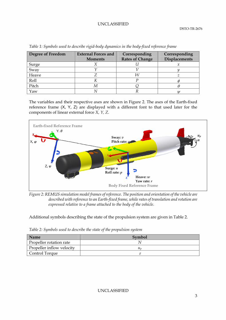
Surge X U x Sway Y V y Heave Z W z Roll K P Pitch M Q Yaw N R The variables and their respective axes are shown in Figure 2. The axes of the Earth-fixed reference frame (X, Y, Z) are displayed with a different font to that used later for the components of linear external force X, Y, Z.
Figure 2: REMUS simulation model frames of reference. The position and orientation of the vehicle are
described with reference to an Earth-fixed frame, while rates of translation and rotation are expressed relative to a frame attached to the body of the vehicle.
Y, θ
X, φ
Z, ψ
Heave: w Yaw rate: r
Sway: v Pitch rate: q
Surge: u Roll rate: p
Earth-fixed Reference Frame
Body Fixed Reference Frame
z
up n
Additional symbols describing the state of the propulsion system are given in Table 2.
Table 2: Symbols used to describe the state of the propulsion system
Name Symbol Propeller rotation rate N Propeller inflow velocity up Control Torque
UNCLASSIFIED 3
UNCLASSIFIED DSTO-TR-2576
2.2.2 Mathematical Representation
The vehicle’s ‘state’ at any instant in time is described mathematically by a state vector, incorporating its rates of translation and rotation, its absolute orientation and position, and the status of its propulsion system: (2.2.1a) ,][ T
punrqpwvu ZYXΞ
where ‘T’ denotes the transpose operator. The velocity components of the vehicle can also be described relative to the water flow as (V, α, β) (see Section 2.3.2), giving rise to the alternative state vector (2.2.1b) .][ T
punrqpV ZYXΞ
The vehicle’s control state is likewise described by a control input vector,
(2.2.2) .Trs u
This vector comprises the elevator angle δs, the rudder angle δr and the mechanical torque the motor exerts around the propeller axis, . The mathematical model of the vehicle is implemented in the form of a function which takes the vehicle state and the control input in the form of vectors and u and predicts the rate of the change of each of the vehicle state variables in the form (2.2.3) .),(),()( tttft uΞΞ The components of the rate of change equations are given in Section 2.4. 2.3 Coordinate Transformations
2.3.1 Earth and Body Reference Frames
The equations in Section 2.4 describe the vehicle state in the body-fixed frame of reference. Thus, transformations are necessary to move between body-fixed and earth-fixed coordinate
systems. The linear velocity components in the earth-fixed reference frame are related to the body-frame velocity components by:
),,( ZYX ,,( vu )w
(2.3.1) )cossincossin(sin
)sinsincoscossin(coscos
w
vuX
UNCLASSIFIED 4
UNCLASSIFIED DSTO-TR-2676
(2.3.2) )cossinsinsincos(
)sinsinsincos(coscossin
w
vuY
(2.3.3) coscossincossin wvu Z The rate equations for the earth-fixed Euler angles ),,( are similarly expressed in terms of the body-fixed rates of turn by: ),,( rqp sin tan cos tanp q r (2.3.4)
cos sinq r (2.3.5)
sin cos cos cosq r (2.3.6) 2.3.2 Body and Stability Reference Frames
For convenience of interpretation, the vehicle state is projected into the so-called ‘stability’ reference frame; that is, the reference frame attached to the body of water surrounding the vehicle, which in the absence of current is identical to the earth-fixed reference frame. In this case, the body-axis velocity components (u, v, w) are replaced by the forward speed, angle of attack and sideslip angle (V, α, β), defined by
222 wvuV (2.3.7)
uw1tan (2.3.8)
Vv1sin (2.3.9) Equivalently, coscosVu (2.3.10) sinVv (2.3.11) cossinVw (2.3.12) The rates of change of the stability variables are given in terms of the rates of change of quantities expressed in the body-frame by the following equations:
cos cos sin sin cosV u v w (2.3.13)
cos
sincos
V
uw (2.3.14)
1cos cos sin sin sinv u w
V (2.3.15)
UNCLASSIFIED 5
UNCLASSIFIED DSTO-TR-2576
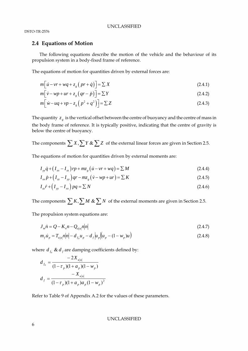
2.4 Equations of Motion
The following equations describe the motion of the vehicle and the behaviour of its propulsion system in a body-fixed frame of reference. The equations of motion for quantities driven by external forces are:
(2.4.1) gm u vr wq z pr q X
(2.4.2) gm v wp ur z qr p Y
(2.4.3) 2 2gm w uq vp z p q Z
The quantity is the vertical offset between the centre of buoyancy and the centre of mass in
the body frame of reference. It is typically positive, indicating that the centre of gravity is below the centre of buoyancy.
gz
The components of the external linear forces are given in Section ZYX &, 2.5.
The equations of motion for quantities driven by external moments are: yy xx zz gI q I I rp mz u vr wq M (2.4.4)
xx zz yy gI p I I qr mz v wp ur K (2.4.5)
zz yy xxI r I I pq N (2.4.6)
The components of the external moments are given in Section NMK &, 2.5.
The propulsion system equations are: nnQnKQnJ nnnm (2.4.7)
uwuududnnTum pppfpfnnpf )1(0
(2.4.8)
where are damping coefficients defined by: ff dd &
0
)1)(1)(1(
20
ppp
uu
f wa
Xd
2)1()1)(1( pppp
uu
f waa
Xd
Refer to Table 9 of Appendix A.2 for the values of these parameters.
UNCLASSIFIED 6
UNCLASSIFIED DSTO-TR-2676
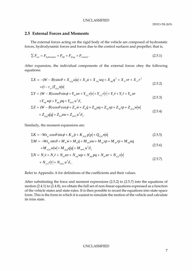
2.5 External Forces and Moments
The external forces acting on the rigid body of the vehicle are composed of hydrostatic forces, hydrodynamic forces and forces due to the control surfaces and propeller; that is, . (2.5.1) ext hydrostatic lift drag controlF F F F F After expansion, the individual components of the external forces obey the following equations:
nnT
rXvrXqXwqXuXuuXBWX
nnp
rrvrqqwquuu
)1(
sin)( 22
(2.5.2)
ruupqwp
urrvrrvvuv
uYpqYwpY
urYrYvYrrYvvYuvYBWY
r
2
sincos)(
(2.5.3)
.
coscos)(
2suuuwqq
wwrpvpuqqw
uZuwZqqZ
wwZrpZvpZuqZqZwZBWZ
s
(2.5.4)
Similarly, the moment expansions are: nnQppKpKWzK nnpppg ||sincos (2.5.5)
suuqqww
uqrpvpuwqwg
uMqqMwwM
uqMrpMvpMuwMqMwMWzM
s
2
sin
(2.5.6)
.2
ruurr
vvurpqwpuvrv
uNrrN
vvNurNpqNwpNuvNrNvNN
r
(2.5.7)
Refer to Appendix A for definitions of the coefficients and their values. After substituting the force and moment expressions (2.5.2) to (2.5.7) into the equations of motion (2.4.1) to (2.4.8), we obtain the full set of non-linear equations expressed as a function of the vehicle states and state-rates. It is then possible to recast the equations into state-space form. This is the form in which it is easiest to simulate the motion of the vehicle and calculate its trim state.
UNCLASSIFIED 7
UNCLASSIFIED DSTO-TR-2576
3. Estimation of Trim
3.1 Definition of Trim
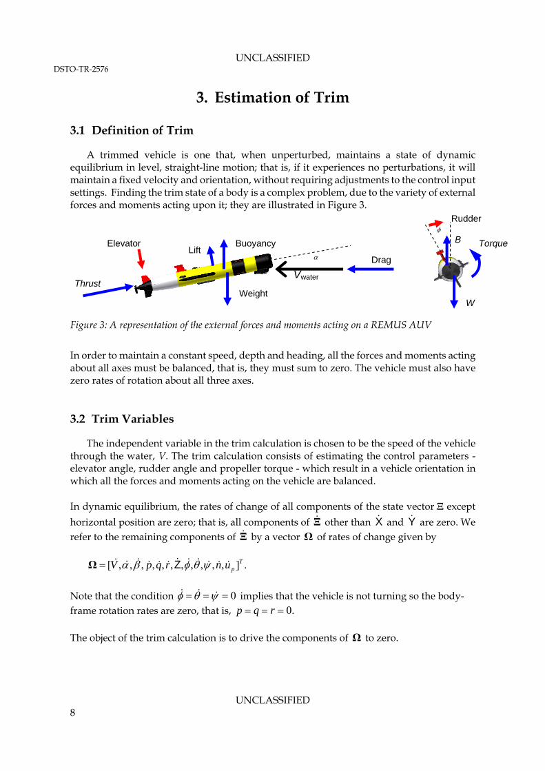
A trimmed vehicle is one that, when unperturbed, maintains a state of dynamic equilibrium in level, straight-line motion; that is, if it experiences no perturbations, it will maintain a fixed velocity and orientation, without requiring adjustments to the control input settings. Finding the trim state of a body is a complex problem, due to the variety of external forces and moments acting upon it; they are illustrated in Figure 3.
Rudder
B
W
Figure 3: A representation of the external forces and moments acting on a REMUS AUV
In order to maintain a constant speed, depth and heading, all the forces and moments acting about all axes must be balanced, that is, they must sum to zero. The vehicle must also have zero rates of rotation about all three axes. 3.2 Trim Variables
The independent variable in the trim calculation is chosen to be the speed of the vehicle through the water, V. The trim calculation consists of estimating the control parameters - elevator angle, rudder angle and propeller torque - which result in a vehicle orientation in which all the forces and moments acting on the vehicle are balanced. In dynamic equilibrium, the rates of change of all components of the state vector except
horizontal position are zero; that is, all components of Ξ other than and are zero. We refer to the remaining components of Ξ by a vector Ω of rates of change given by
X Y
.],,,,,,,,,,,[ TpunrqpV ZΩ
Note that the condition implies that the vehicle is not turning so the body-frame rotation rates are zero, that is,
0 .0 rqp
The object of the trim calculation is to drive the components of to zero. Ω
Drag
Vwater Thrust
Lift
Weight
Buoyancy Elevator Torque
UNCLASSIFIED 8
UNCLASSIFIED DSTO-TR-2676
3.3 Decision Variables
A set of decision variables must be chosen to facilitate the trim calculation. In this case, for a required forward speed V, the variables chosen are .],,,,,,,,[ T
rspun x This set does not include the linear velocities (u, v, w), because the information they represent is present in the values of (V, α, β); inclusion of (u, v, w) results in an over-determined system. 3.4 Trim Estimation by Numerical Iteration
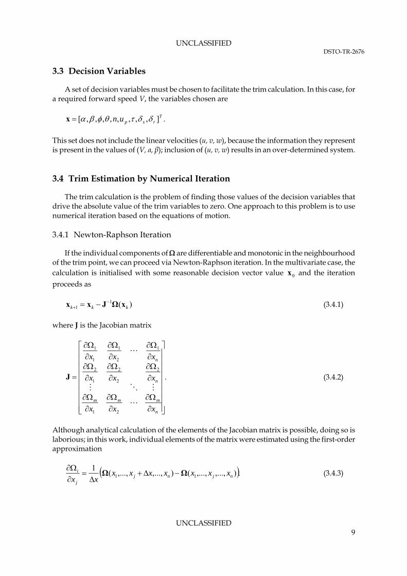
The trim calculation is the problem of finding those values of the decision variables that drive the absolute value of the trim variables to zero. One approach to this problem is to use numerical iteration based on the equations of motion. 3.4.1 Newton-Raphson Iteration
If the individual components of are differentiable and monotonic in the neighbourhood of the trim point, we can proceed via Newton-Raphson iteration. In the multivariate case, the calculation is initialised with some reasonable decision vector value and the iteration
proceeds as 0x
(3.4.1) )(1
1 kkk xΩJxx
where J is the Jacobian matrix
.
21
2
2
2
1
2
1
2
1
1
1
n
mmm
n
n
xxx
xxx
xxx
J (3.4.2)
Although analytical calculation of the elements of the Jacobian matrix is possible, doing so is laborious; in this work, individual elements of the matrix were estimated using the first-order approximation
.),...,,...,(),...,,...,(1
11 njnjj
i xxxxxxxxx
ΩΩ
(3.4.3)
UNCLASSIFIED 9
UNCLASSIFIED DSTO-TR-2576
The convergence of the algorithm is measured by comparing the difference between the current trim vector and the previous trim vector, referred to as the ‘error’, ε
kkk xx 1 (3.4.4)
The iteration was terminated when error was less than a desired tolerance value, ,tol
tol . (3.4.5)
In the following sections of this work, the first-order approximation to the partial derivatives in the Jacobian matrix was calculated with a uniform perturbation value of (3.4.6) .001.0x The iteration was terminated when the absolute difference between successive estimates fell below (3.4.7) .10 10tol Alternatively, the iteration was deemed to have failed to converge if the number of iterations reached 100. 3.4.2 Implementation
The trim method described above was implemented as an algorithm in MATLAB code as the function ‘trim.m’. It takes the following inputs:-
Desired trim speed V and Initial trim state estimate x0 (optional)
The function outputs are:-
The trim state vector x, The number of iterations required to reach to error tolerance, and The final error ε.
The trim function calls a function ‘eom.m’ that implements the state-space form of the equations of motion. The implementation is detailed in Appendix B. 3.4.3 Performance of the Newton-Raphson Iteration
As a case study, Sgarioto [2] reports the trim state for of the REMUS 100 model using parameters given in Appendix A, at the representative forward speed value of V = 4 knots. The values derived by Sgarioto were calculated using a commercial optimisation software package called SNOPT. For comparison, the Newton-Raphson iteration algorithm described in Section 3.4.1 was initialised using the starting value given by Sgarioto [2]:
UNCLASSIFIED 10
UNCLASSIFIED DSTO-TR-2676
(3.4.8) 0 0 0 0 0 0 0 0 0 0[ , , , , , , , , ] [0,0,0,0,76 ,0.9 ,39 ,0,0].Tp s rn u V V V x
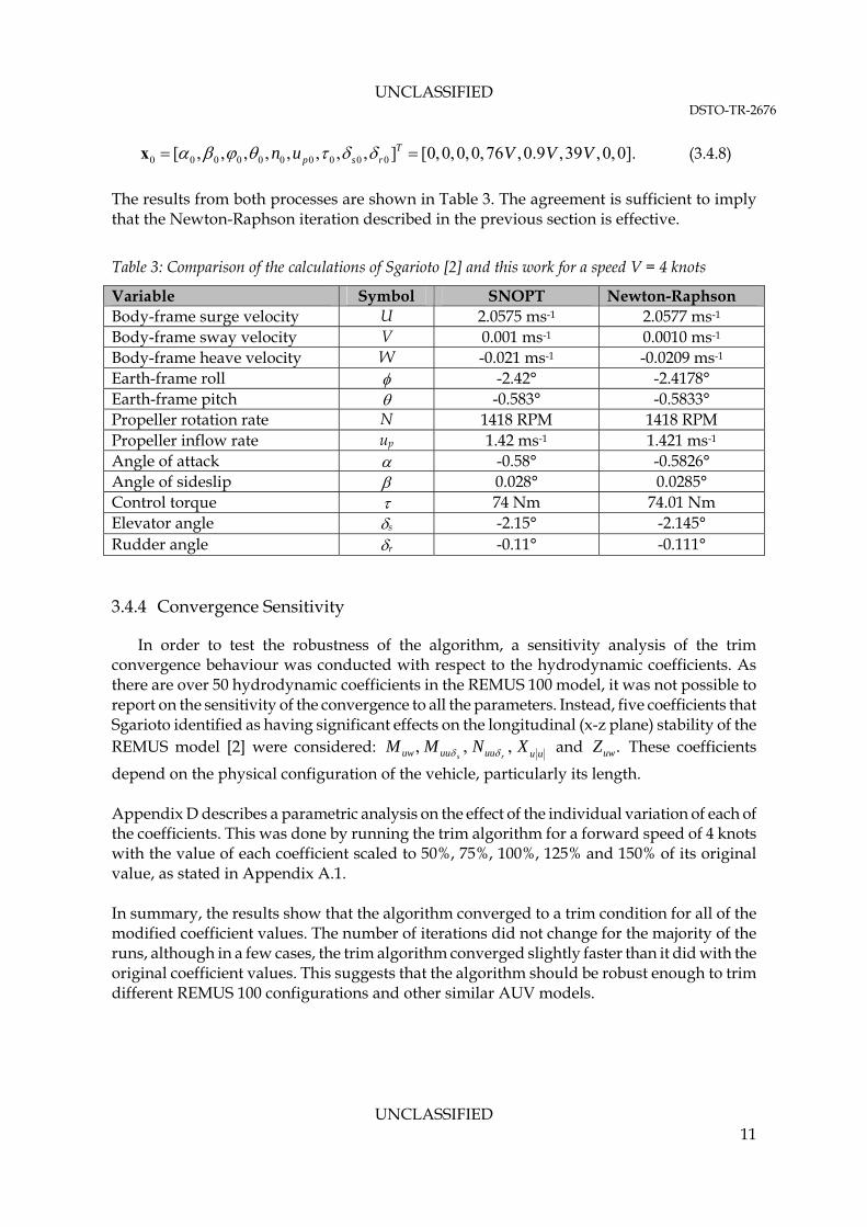
The results from both processes are shown in Table 3. The agreement is sufficient to imply that the Newton-Raphson iteration described in the previous section is effective.
Table 3: Comparison of the calculations of Sgarioto [2] and this work for a speed V = 4 knots
Variable Symbol SNOPT Newton-Raphson Body-frame surge velocity U 2.0575 ms-1 2.0577 ms-1
Body-frame sway velocity V 0.001 ms-1 0.0010 ms-1
Body-frame heave velocity W -0.021 ms-1 -0.0209 ms-1 Earth-frame roll -2.42° -2.4178° Earth-frame pitch -0.583° -0.5833° Propeller rotation rate N 1418 RPM 1418 RPM Propeller inflow rate up 1.42 ms-1 1.421 ms-1 Angle of attack -0.58° -0.5826° Angle of sideslip 0.028° 0.0285° Control torque 74 Nm 74.01 Nm Elevator angle s -2.15° -2.145° Rudder angle r -0.11° -0.111° 3.4.4 Convergence Sensitivity
In order to test the robustness of the algorithm, a sensitivity analysis of the trim convergence behaviour was conducted with respect to the hydrodynamic coefficients. As there are over 50 hydrodynamic coefficients in the REMUS 100 model, it was not possible to report on the sensitivity of the convergence to all the parameters. Instead, five coefficients that Sgarioto identified as having significant effects on the longitudinal (x-z plane) stability of the REMUS model [2] were considered: uuuuuuuw XNMM
rs,,, and These coefficients
depend on the physical configuration of the vehicle, particularly its length.
.uwZ
Appendix D describes a parametric analysis on the effect of the individual variation of each of the coefficients. This was done by running the trim algorithm for a forward speed of 4 knots with the value of each coefficient scaled to 50%, 75%, 100%, 125% and 150% of its original value, as stated in Appendix A.1. In summary, the results show that the algorithm converged to a trim condition for all of the modified coefficient values. The number of iterations did not change for the majority of the runs, although in a few cases, the trim algorithm converged slightly faster than it did with the original coefficient values. This suggests that the algorithm should be robust enough to trim different REMUS 100 configurations and other similar AUV models.
UNCLASSIFIED 11
UNCLASSIFIED DSTO-TR-2576
3.5 Estimation of the Starting Point for the Iteration
The convergence of the Newton-Raphson zero-finding algorithm expressed by equation (3.4.1) can only be guaranteed for a restricted class of functions and starting points for the iteration [3]. For example, the algorithm may fail to find the global minimum if the starting point is close to a local minimum. In the present case, the existence of local minima is difficult to predict, particularly because the parameters of the model depend on the configuration of the vehicle being modeled. This suggests that it is important to select an appropriate starting point for the iteration in order to guarantee convergence to the global minimum. This section considers methods by which a starting point for the iteration can be derived. 3.5.1 Empirical and Analytical Starting Points
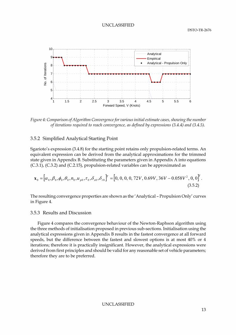
Sgarioto [2] derived equation (3.4.8) for the starting point of the numerical solution of the trim equations empirically, by a process of trial and error that was based on repeatedly integrating the non-linear equations of motion described in Section 2.4 and observing the dynamics of the vehicle as they evolved over long spans of time. Equation (3.4.8) is an appropriate starting point for the Newton-Raphson iteration for forward speeds from 1 knot to 6 knots, with convergence properties shown as the ‘Empirical’ curves in Figure 4. Although it was successful in this case, equation (3.4.8) was derived for a particular set of model parameters and it may not be appropriate for different values of the model parameters. It is possible to derive more widely applicable initial conditions from first principles. By applying a set of steady, level flight assumptions to the vehicle force balance equations and approximating the equations by neglecting terms smaller than second order in small quantities, it is possible to obtain analytical expressions for the trim state of the vehicle. The derivation and form of these analytical expressions are described in Appendix C. Although the analytical approximations of the trimmed state given as expressions (C.2.15) to (C.3.8) in Appendix C are not sufficiently accurate for use in trim-based calculations over the full range of vehicle speeds2, they are appropriate starting points for iterative refinement. The convergence properties that result from using these expressions as the starting points for the Newton-Raphson iteration are shown as the ‘Analytical’ curves in Figure 4.
2 The approximations were found to predict all trim state variables within 1% of the iterative benchmark values for forward speeds above 2.9 knots; as the vehicle speed decreased, the approximation became increasingly inaccurate, with some decision variables diverging more than 25% from the iterative solution (see Appendix C.4 for details of the comparison).
UNCLASSIFIED 12
UNCLASSIFIED DSTO-TR-2676
1 1.5 2 2.5 3 3.5 4 4.5 5 5.5 64
5
6
7
8
9
10N
o. o
f It
erat
ions
Forward Speed, V (Knots)
Analytical
EmpiricalAnalytical - Propulsion Only
Figure 4: Comparison of Algorithm Convergence for various initial estimate cases, showing the number
of iterations required to reach convergence, as defined by expressions (3.4.4) and (3.4.5).
3.5.2 Simplified Analytical Starting Point
Sgarioto’s expression (3.4.8) for the starting point retains only propulsion-related terms. An equivalent expression can be derived from the analytical approximations for the trimmed state given in Appendix B. Substituting the parameters given in Appendix A into equations (C.3.1), (C.3.2) and (C.2.15), propulsion-related variables can be approximated as
.0,0,058.036,69.0,72,0,0,0,0,,,,,,,, 20000000000
TTrsp VVVVun x
(3.5.2) The resulting convergence properties are shown as the ‘Analytical – Propulsion Only’ curves in Figure 4. 3.5.3 Results and Discussion
Figure 4 compares the convergence behaviour of the Newton-Raphson algorithm using the three methods of initialisation proposed in previous sub-sections. Initialisation using the analytical expressions given in Appendix B results in the fastest convergence at all forward speeds, but the difference between the fastest and slowest options is at most 40% or 4 iterations; therefore it is practically insignificant. However, the analytical expressions were derived from first principles and should be valid for any reasonable set of vehicle parameters; therefore they are to be preferred.
UNCLASSIFIED 13
UNCLASSIFIED DSTO-TR-2576
4. Parametric Study
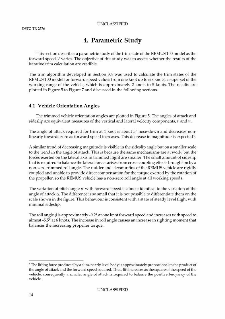
This section describes a parametric study of the trim state of the REMUS 100 model as the forward speed V varies. The objective of this study was to assess whether the results of the iterative trim calculation are credible. The trim algorithm developed in Section 3.4 was used to calculate the trim states of the REMUS 100 model for forward speed values from one knot up to six knots, a superset of the working range of the vehicle, which is approximately 2 knots to 5 knots. The results are plotted in Figure 5 to Figure 7 and discussed in the following sections. 4.1 Vehicle Orientation Angles
The trimmed vehicle orientation angles are plotted in Figure 5. The angles of attack and sideslip are equivalent measures of the vertical and lateral velocity components, v and w. The angle of attack required for trim at 1 knot is about 5° nose-down and decreases non-linearly towards zero as forward speed increases. This decrease in magnitude is expected3. A similar trend of decreasing magnitude is visible in the sideslip angle but on a smaller scale to the trend in the angle of attack. This is because the same mechanisms are at work, but the forces exerted on the lateral axis in trimmed flight are smaller. The small amount of sideslip that is required to balance the lateral forces arises from cross-coupling effects brought on by a non-zero trimmed roll angle. The rudder and elevator fins of the REMUS vehicle are rigidly coupled and unable to provide direct compensation for the torque exerted by the rotation of the propeller, so the REMUS vehicle has a non-zero roll angle at all working speeds. The variation of pitch angle with forward speed is almost identical to the variation of the angle of attack . The difference is so small that it is not possible to differentiate them on the scale shown in the figure. This behaviour is consistent with a state of steady level flight with minimal sideslip. The roll angle is approximately -0.2° at one knot forward speed and increases with speed to almost -5.5° at 6 knots. The increase in roll angle causes an increase in righting moment that balances the increasing propeller torque.
3 The lifting force produced by a slim, nearly level body is approximately proportional to the product of the angle of attack and the forward speed squared. Thus, lift increases as the square of the speed of the vehicle; consequently a smaller angle of attack is required to balance the positive buoyancy of the vehicle.
UNCLASSIFIED 14
UNCLASSIFIED DSTO-TR-2676
1 1.5 2 2.5 3 3.5 4 4.5 5 5.5 6-6
-4
-2
0
, (
o )
1 1.5 2 2.5 3 3.5 4 4.5 5 5.5 60.025
0.03
0.035
0.04
, (
o )
1 1.5 2 2.5 3 3.5 4 4.5 5 5.5 6-6
-4
-2
0
, (
o )
Forward Speed, V (Knots)
Figure 5: Variation of trimmed angle of attack/pitch angle (top), sideslip angle (middle) and roll angle (bottom) with forward speed
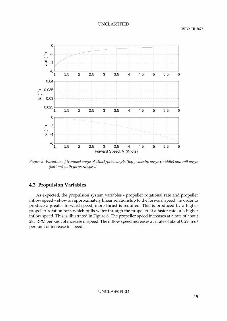
4.2 Propulsion Variables
As expected, the propulsion system variables - propeller rotational rate and propeller inflow speed – show an approximately linear relationship to the forward speed. In order to produce a greater forward speed, more thrust is required. This is produced by a higher propeller rotation rate, which pulls water through the propeller at a faster rate or a higher inflow speed. This is illustrated in Figure 6. The propeller speed increases at a rate of about 285 RPM per knot of increase in speed. The inflow speed increases at a rate of about 0.29 ms-1 per knot of increase in speed.
UNCLASSIFIED 15
UNCLASSIFIED DSTO-TR-2576
1 1.5 2 2.5 3 3.5 4 4.5 5 5.5 60
100
200
300
Forward Speed, V (Knots)
n,
( R
PM
)
1 1.5 2 2.5 3 3.5 4 4.5 5 5.5 60
1
2
3
Forward Speed, V (Knots)
up,
(m/s
)
Figure 6: Variation of propulsion system state variables propeller rotation rate (top) and propeller
inflow speed
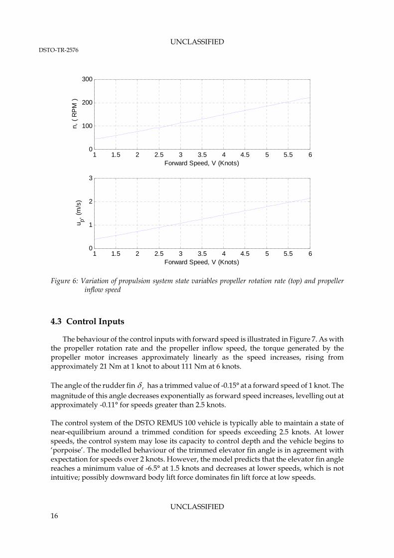
4.3 Control Inputs
The behaviour of the control inputs with forward speed is illustrated in Figure 7. As with the propeller rotation rate and the propeller inflow speed, the torque generated by the propeller motor increases approximately linearly as the speed increases, rising from approximately 21 Nm at 1 knot to about 111 Nm at 6 knots. The angle of the rudder fin r has a trimmed value of -0.15° at a forward speed of 1 knot. The magnitude of this angle decreases exponentially as forward speed increases, levelling out at approximately -0.11° for speeds greater than 2.5 knots. The control system of the DSTO REMUS 100 vehicle is typically able to maintain a state of near-equilibrium around a trimmed condition for speeds exceeding 2.5 knots. At lower speeds, the control system may lose its capacity to control depth and the vehicle begins to ‘porpoise’. The modelled behaviour of the trimmed elevator fin angle is in agreement with expectation for speeds over 2 knots. However, the model predicts that the elevator fin angle reaches a minimum value of -6.5° at 1.5 knots and decreases at lower speeds, which is not intuitive; possibly downward body lift force dominates fin lift force at low speeds.
UNCLASSIFIED 16
UNCLASSIFIED DSTO-TR-2676
1 1.5 2 2.5 3 3.5 4 4.5 5 5.5 6-10
-5
0 s
,( o )
1 1.5 2 2.5 3 3.5 4 4.5 5 5.5 6-0.16
-0.14
-0.12
-0.1
r,(
o )
1 1.5 2 2.5 3 3.5 4 4.5 5 5.5 60
50
100
150
(N
m)
Forward Speed, V (Knots)
Figure 7: Variation of trimmed control input settings elevator fin angle (top), rudder fin angle (middle) and propeller motor mechanical torque (bottom) with forward speed.
In summary, the numerical trim algorithm converges over a wider range of speeds than those at which the physical vehicle operates. The predicted behaviour of the trimmed vehicle states is in agreement with expectation for speeds over two knots. The predicted behaviour of the trimmed elevator fin angle at speeds under 2 knots is not intuitive, but it is beyond the range that can be checked by reference to the behaviour of the physical vehicle.
5. Conclusion
The calculations given in this work demonstrate that the REMUS 100 vehicle dynamics model described by Prestero [1] and extended by Sgarioto [4] is readily trimmed using a numerical zero-finding procedure based on Newton-Raphson iteration. This work also presents analytical approximations to the trimmed state that can be used as a starting point for numerical procedure. With suitable parameters, the procedure should be adjustable to model different REMUS 100 configurations and vehicles of similar size and shape.
UNCLASSIFIED 17
UNCLASSIFIED DSTO-TR-2576
6. References
1. Prestero, T. “Verification of a Six-Degree-of-Freedom Simulation Model for the REMUS Autonomous Underwater Vehicle”, MSc/ME Thesis, Massachusetts Institute of Technology, Sept. 2001
2. Sgarioto, D. “Steady State Trim and Open Loop Stability Analysis for the REMUS Autonomous Underwater Vehicle”, Defence Technology Agency, New Zealand Defence Force, DTA Report 254, March 2008.
3. Press, W. H., Teukolksy, S. A., Vetterling, W. T. and Flannery, B. P. (1992)
Numerical Recipes in C, 3rd Edition, Cambridge University Press.
4. Sgarioto, D. “Control System Design and Development for the REMUS Autonomous Underwater Vehicle”, Defence Technology Agency, New Zealand Defence Force, DTA Report 250, May 2007.
Acknowledgments This work was motivated by private communications from Dr Daniel Sgarioto, then working at the New Zealand Defence Technology Agency. The Defence Technology Agency also provided Dan’s Matlab implementation of a REMUS 100 dynamical model, some of which is reproduced in this work with their permission.
UNCLASSIFIED 18
UNCLASSIFIED DSTO-TR-2676
Appendix A: REMUS 100 Model Parameters
A.1. Mathematical Symbols
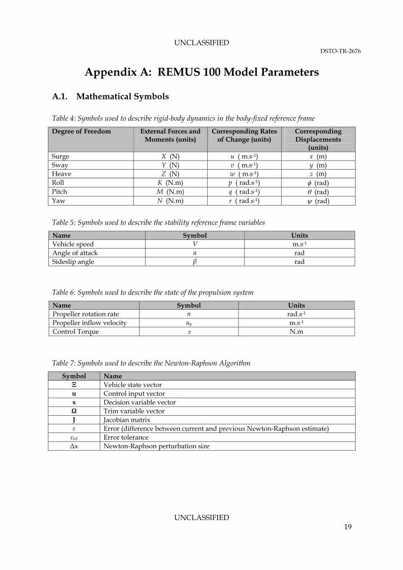
Table 4: Symbols used to describe rigid-body dynamics in the body-fixed reference frame
Degree of Freedom External Forces and Moments (units)
Corresponding Rates of Change (units)
Corresponding Displacements
(units) Surge X (N) u ( m.s-1) x (m) Sway Y (N) v ( m.s-1) y (m) Heave Z (N) w ( m.s-1) z (m) Roll K (N.m) p ( rad.s-1) (rad) Pitch M (N.m) q ( rad.s-1) (rad) Yaw N (N.m) r ( rad.s-1) (rad)
Table 5: Symbols used to describe the stability reference frame variables
Name Symbol Units Vehicle speed V m.s-1 Angle of attack α rad Sideslip angle β rad
Table 6: Symbols used to describe the state of the propulsion system
Name Symbol Units Propeller rotation rate n rad.s-1 Propeller inflow velocity up m.s-1 Control Torque N.m
Table 7: Symbols used to describe the Newton-Raphson Algorithm
Symbol Name Ξ Vehicle state vector u Control input vector x Decision variable vector Ω Trim variable vector J Jacobian matrix ε Error (difference between current and previous Newton-Raphson estimate) εtol Error tolerance Δx Newton-Raphson perturbation size
UNCLASSIFIED 19
UNCLASSIFIED DSTO-TR-2576
A.2. Case Study Parameters
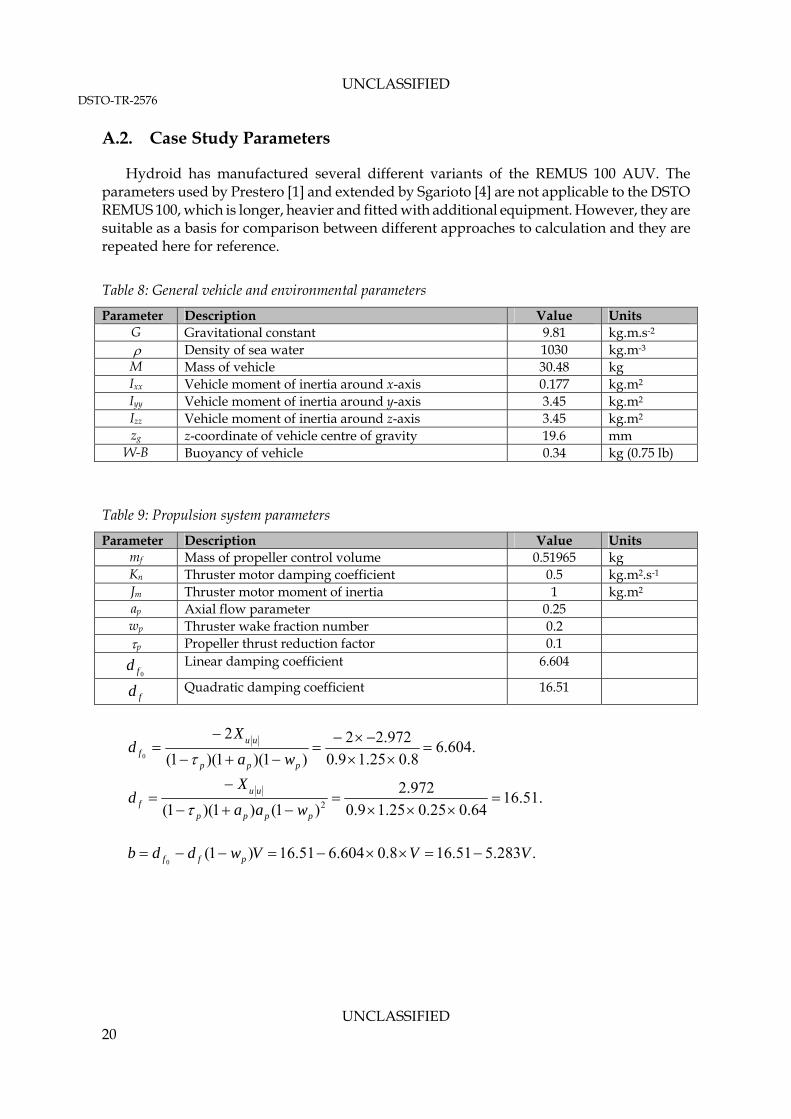
Hydroid has manufactured several different variants of the REMUS 100 AUV. The parameters used by Prestero [1] and extended by Sgarioto [4] are not applicable to the DSTO REMUS 100, which is longer, heavier and fitted with additional equipment. However, they are suitable as a basis for comparison between different approaches to calculation and they are repeated here for reference.
Table 8: General vehicle and environmental parameters
Parameter Description Value Units G Gravitational constant 9.81 kg.m.s-2
Density of sea water 1030 kg.m-3
M Mass of vehicle 30.48 kg Ixx Vehicle moment of inertia around x-axis 0.177 kg.m2
Iyy Vehicle moment of inertia around y-axis 3.45 kg.m2
Izz Vehicle moment of inertia around z-axis 3.45 kg.m2
zg z-coordinate of vehicle centre of gravity 19.6 mm W-B Buoyancy of vehicle 0.34 kg (0.75 lb)
Table 9: Propulsion system parameters
Parameter Description Value Units mf Mass of propeller control volume 0.51965 kg Kn Thruster motor damping coefficient 0.5 kg.m2.s-1
Jm Thruster motor moment of inertia 1 kg.m2
ap Axial flow parameter 0.25 wp Thruster wake fraction number 0.2 p Propeller thrust reduction factor 0.1
0fd Linear damping coefficient 6.604
fd Quadratic damping coefficient 16.51
.604.68.025.19.0
972.22
)1)(1)(1(
20
ppp
uuf wa
Xd
.51.1664.025.025.19.0
972.2
)1()1)(1( 2
pppp
uuf waa
Xd
.283.551.168.0604.651.16)1(
0VVVwddb pff
UNCLASSIFIED 20
UNCLASSIFIED DSTO-TR-2676
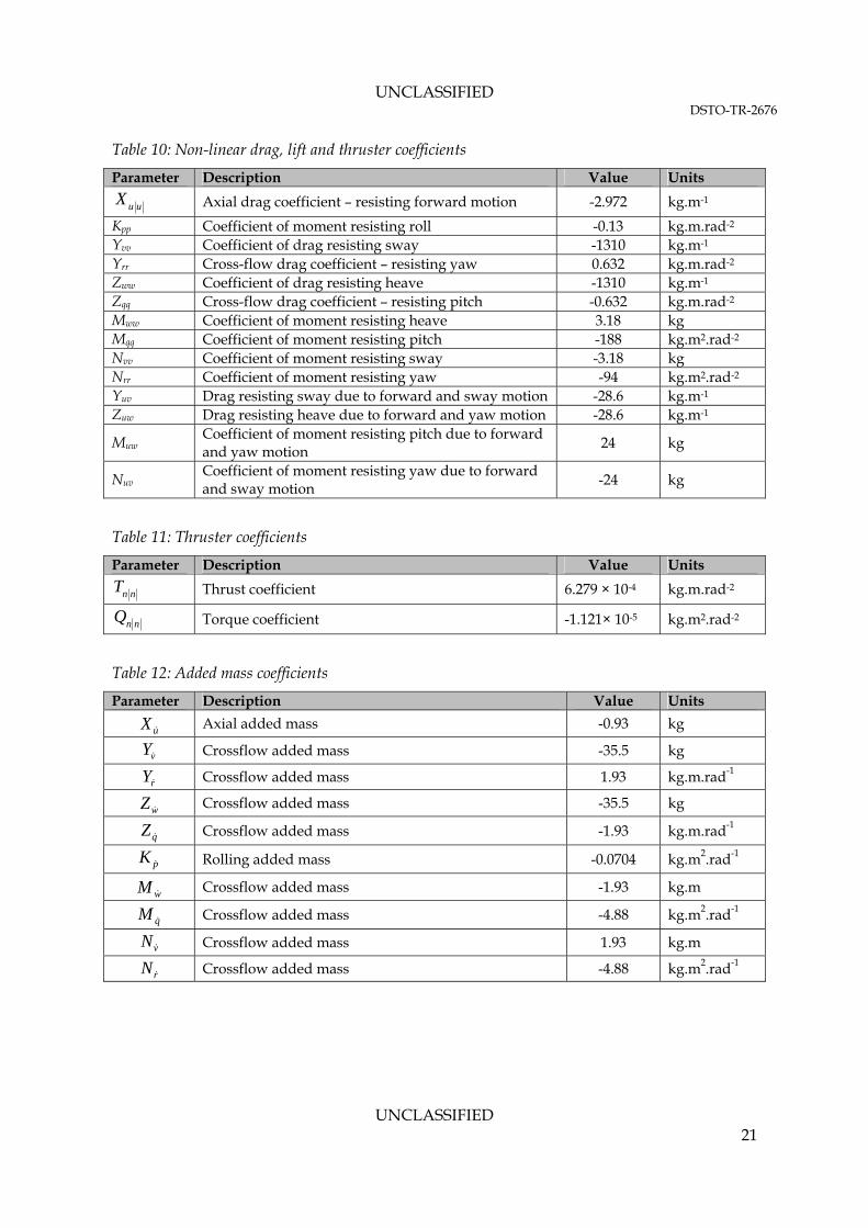
Table 10: Non-linear drag, lift and thruster coefficients
Parameter Description Value Units
uuX Axial drag coefficient – resisting forward motion -2.972 kg.m-1
Kpp Coefficient of moment resisting roll -0.13 kg.m.rad-2
Yvv Coefficient of drag resisting sway -1310 kg.m-1 Yrr Cross-flow drag coefficient – resisting yaw 0.632 kg.m.rad-2 Zww Coefficient of drag resisting heave -1310 kg.m-1 Zqq Cross-flow drag coefficient – resisting pitch -0.632 kg.m.rad-2 Mww Coefficient of moment resisting heave 3.18 kg Mqq Coefficient of moment resisting pitch -188 kg.m2.rad-2 Nvv Coefficient of moment resisting sway -3.18 kg Nrr Coefficient of moment resisting yaw -94 kg.m2.rad-2 Yuv Drag resisting sway due to forward and sway motion -28.6 kg.m-1 Zuw Drag resisting heave due to forward and yaw motion -28.6 kg.m-1
Muw Coefficient of moment resisting pitch due to forward and yaw motion
24 kg
Nuv Coefficient of moment resisting yaw due to forward and sway motion
-24 kg
Table 11: Thruster coefficients
Parameter Description Value Units
nnT Thrust coefficient 6.279 × 10⁻⁴ kg.m.rad-2
nnQ Torque coefficient -1.121× 10⁻⁵ kg.m2.rad-2
Table 12: Added mass coefficients
Parameter Description Value Units
uX Axial added mass -0.93 kg
vY Crossflow added mass -35.5 kg
rY Crossflow added mass 1.93 kg.m.rad-1
wZ Crossflow added mass -35.5 kg
qZ Crossflow added mass -1.93 kg.m.rad-1
pK Rolling added mass -0.0704 kg.m2.rad-1
wM Crossflow added mass -1.93 kg.m
qM Crossflow added mass -4.88 kg.m2.rad-1
vN Crossflow added mass 1.93 kg.m
rN Crossflow added mass -4.88 kg.m2.rad-1
UNCLASSIFIED 21
UNCLASSIFIED DSTO-TR-2576
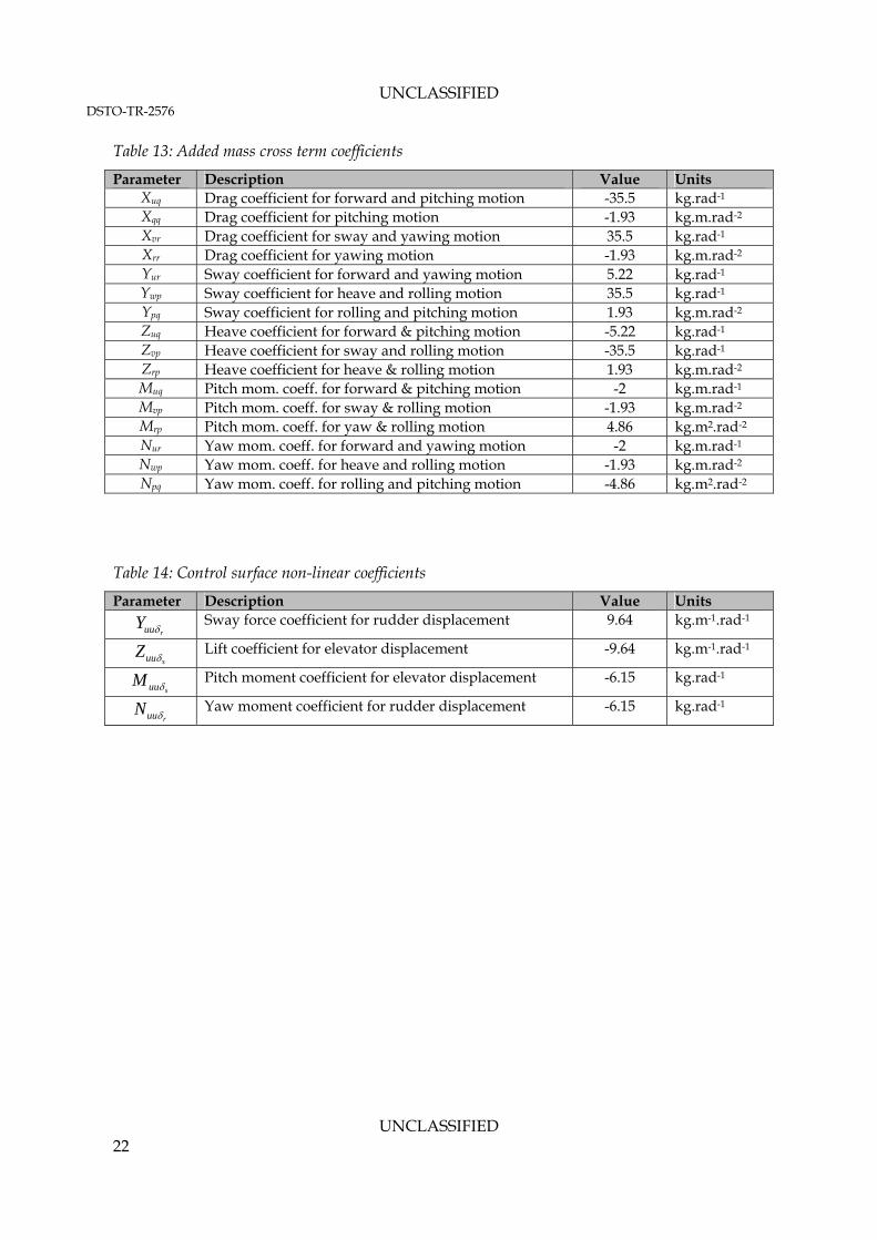
Table 13: Added mass cross term coefficients
Parameter Description Value Units Xuq Drag coefficient for forward and pitching motion -35.5 kg.rad-1
Xqq Drag coefficient for pitching motion -1.93 kg.m.rad-2 Xvr Drag coefficient for sway and yawing motion 35.5 kg.rad-1 Xrr Drag coefficient for yawing motion -1.93 kg.m.rad-2 Yur Sway coefficient for forward and yawing motion 5.22 kg.rad-1 Ywp Sway coefficient for heave and rolling motion 35.5 kg.rad-1 Ypq Sway coefficient for rolling and pitching motion 1.93 kg.m.rad-2 Zuq Heave coefficient for forward & pitching motion -5.22 kg.rad-1 Zvp Heave coefficient for sway and rolling motion -35.5 kg.rad-1 Zrp Heave coefficient for heave & rolling motion 1.93 kg.m.rad-2 Muq Pitch mom. coeff. for forward & pitching motion -2 kg.m.rad-1 Mvp Pitch mom. coeff. for sway & rolling motion -1.93 kg.m.rad-2 Mrp Pitch mom. coeff. for yaw & rolling motion 4.86 kg.m2.rad-2 Nur Yaw mom. coeff. for forward and yawing motion -2 kg.m.rad-1 Nwp Yaw mom. coeff. for heave and rolling motion -1.93 kg.m.rad-2 Npq Yaw mom. coeff. for rolling and pitching motion -4.86 kg.m2.rad-2
Table 14: Control surface non-linear coefficients
Parameter Description Value Units
ruuY Sway force coefficient for rudder displacement 9.64 kg.m-1.rad-1
suuZ Lift coefficient for elevator displacement -9.64 kg.m-1.rad-1
suuM Pitch moment coefficient for elevator displacement -6.15 kg.rad-1
ruuN Yaw moment coefficient for rudder displacement -6.15 kg.rad-1
UNCLASSIFIED 22
UNCLASSIFIED DSTO-TR-2676
Appendix B: Algorithm Implementation
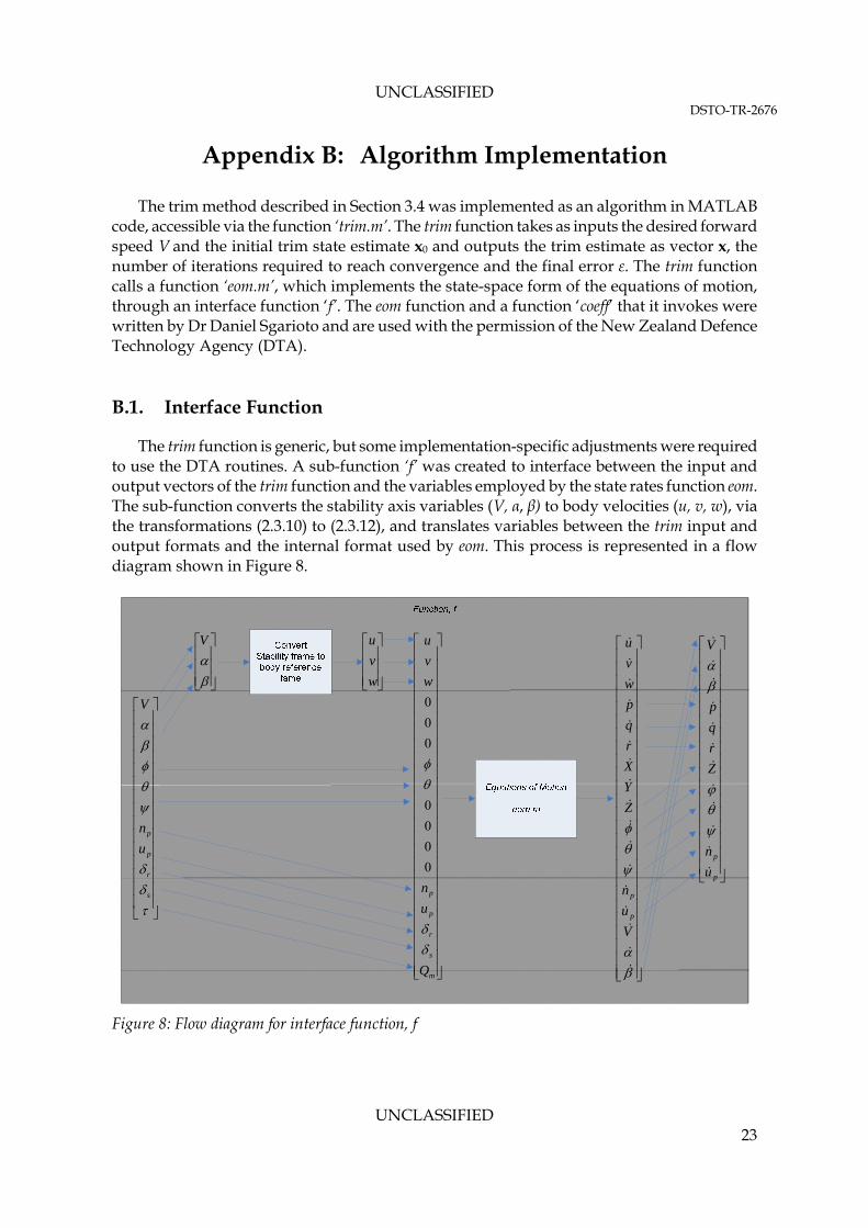
The trim method described in Section 3.4 was implemented as an algorithm in MATLAB code, accessible via the function ‘trim.m’. The trim function takes as inputs the desired forward speed V and the initial trim state estimate x0 and outputs the trim estimate as vector x, the number of iterations required to reach convergence and the final error ε. The trim function calls a function ‘eom.m’, which implements the state-space form of the equations of motion, through an interface function ‘f’. The eom function and a function ‘coeff’ that it invokes were written by Dr Daniel Sgarioto and are used with the permission of the New Zealand Defence Technology Agency (DTA). B.1. Interface Function
The trim function is generic, but some implementation-specific adjustments were required to use the DTA routines. A sub-function ‘f’ was created to interface between the input and output vectors of the trim function and the variables employed by the state rates function eom. The sub-function converts the stability axis variables (V, α, β) to body velocities (u, v, w), via the transformations (2.3.10) to (2.3.12), and translates variables between the trim input and output formats and the internal format used by eom. This process is represented in a flow diagram shown in Figure 8.
V
w
v
u
m
s
r
p
p
Q
u
n
w
v
u
0
0
0
0
0
0
0
s
r
p
p
u
n
V
V
u
n
Z
Y
X
r
q
p
w
v
u
p
p
p
p
u
n
Z
r
q
p
V
Figure 8: Flow diagram for interface function, f
UNCLASSIFIED 23
UNCLASSIFIED DSTO-TR-2576
B.2. Iteration Algorithm
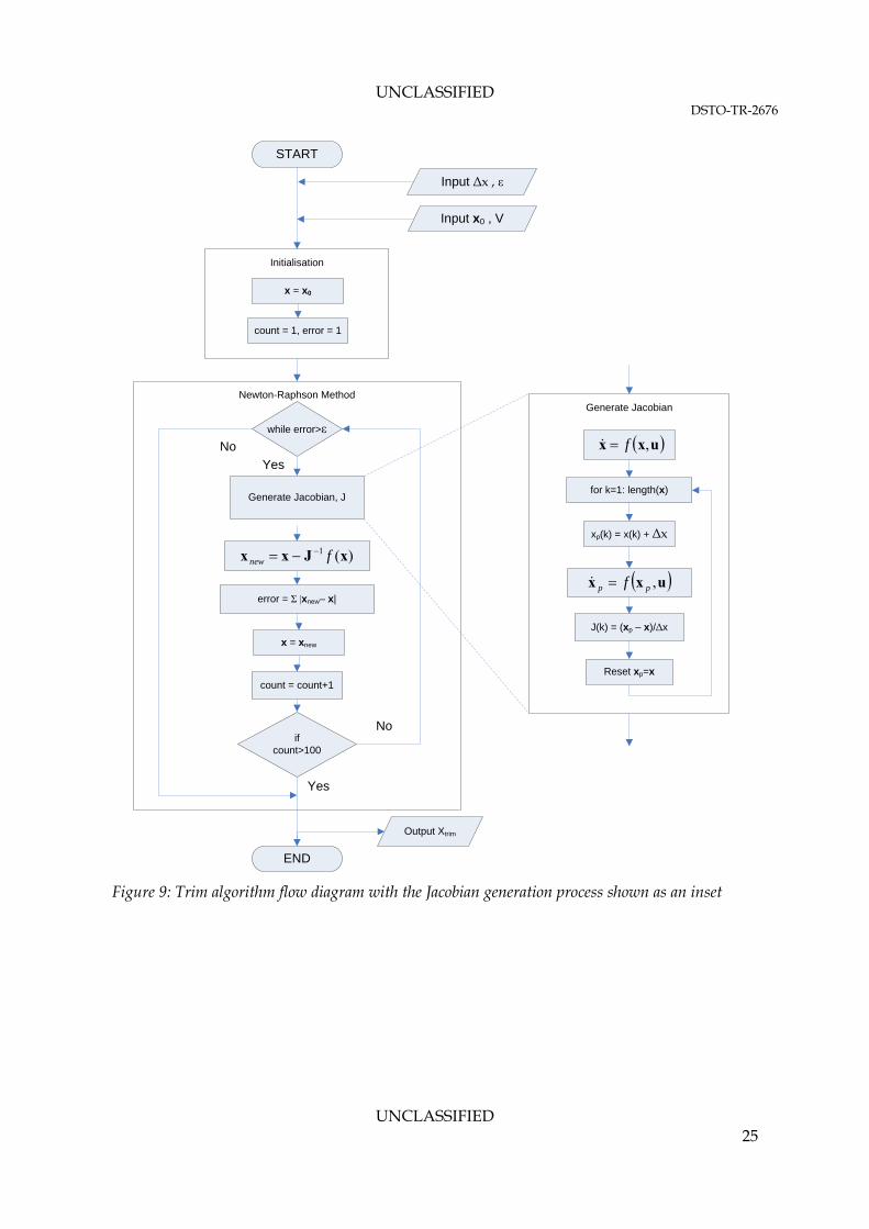
The Newton-Raphson method is implemented in the function ‘trim.m’. The algorithm is designed to trim the equations contained within the interface function ‘f’. The algorithm is split loosely into three sections: algorithm initialisation, the Newton-Raphson iteration and post-processing and display. The Newton-Raphson iteration consists of a while-loop which continues to apply the Newtown-Raphson method while the total difference between the current and previous trim estimates is greater than a preset error tolerance value. There is also a loop break condition if the number of iterations exceeds 100; this is included to stop the algorithm from running indefinitely in the event that a trim point can not be found. A flow diagram representation of the algorithm is shown in Figure 9. B.2.1 Jacobian matrix calculation
The Jacobian matrix is calculated within the state rates interface function f. The process is implemented as a for-loop which cycles through each trim variable. Within each iteration, all the partial derivatives with respect to the trim variable in question are calculated; that is, one column of the Jacobian matrix is calculated at each iteration. A flow diagram representation of the Jacobian generation loop is shown separately within Figure 9.
UNCLASSIFIED 24
UNCLASSIFIED DSTO-TR-2676
Newton-Raphson MethodGenerate Jacobian
for k=1: length(x)
uxx ,pp f
xp(k) = x(k) + Δx
J(k) = (xp – x)/Δx
Reset xp=x
START
Input Δx , ε
Input x0 , V
while error>ε
)(1 xJxx fnew
END
ifcount>100
error = Σ |xnew– x|
count = count+1
Output Xtrim
x = xnew
x = x0
Initialisation
count = 1, error = 1
Yes
No
Yes
No
Generate Jacobian, J
uxx ,f
Figure 9: Trim algorithm flow diagram with the Jacobian generation process shown as an inset
UNCLASSIFIED 25
UNCLASSIFIED DSTO-TR-2576
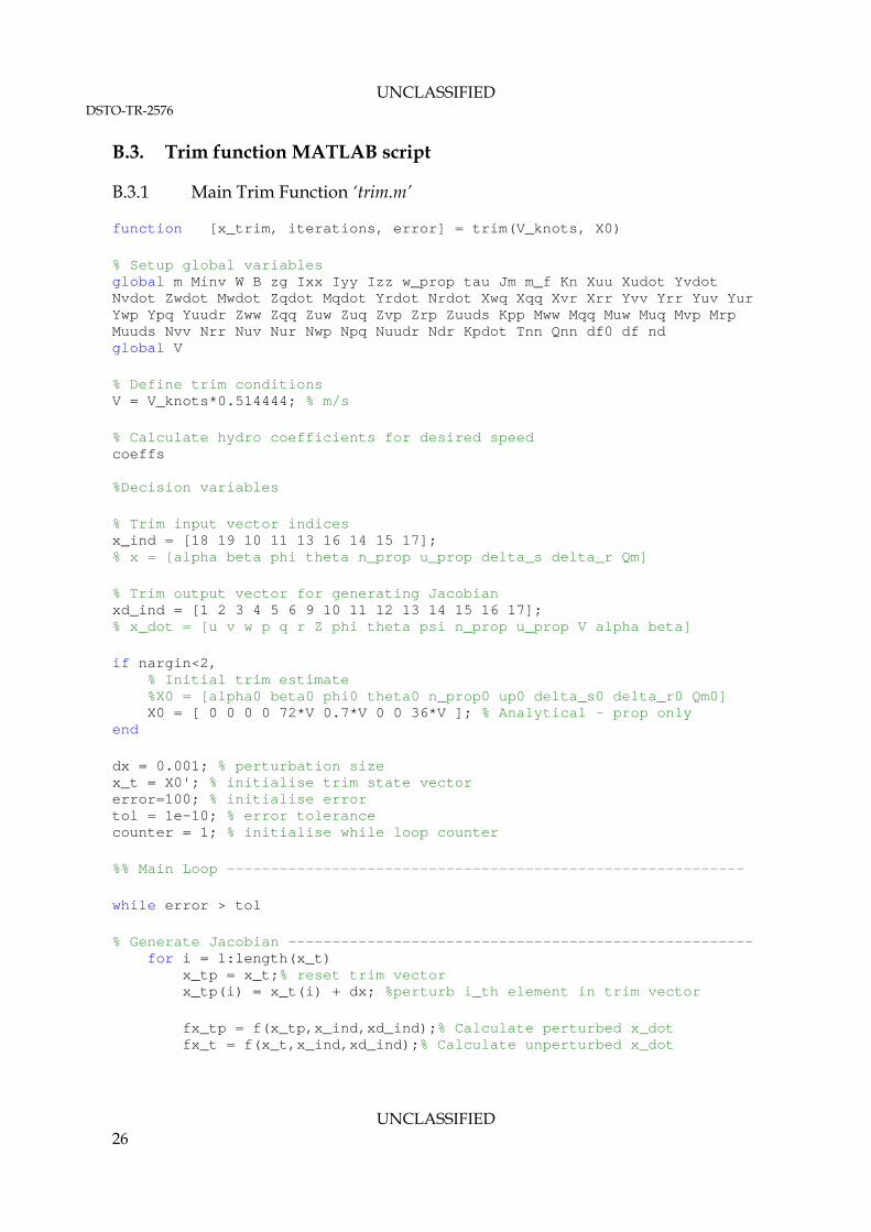
B.3. Trim function MATLAB script
B.3.1 Main Trim Function ‘trim.m’
function [x_trim, iterations, error] = trim(V_knots, X0) % Setup global variables global m Minv W B zg Ixx Iyy Izz w_prop tau Jm m_f Kn Xuu Xudot Yvdot Nvdot Zwdot Mwdot Zqdot Mqdot Yrdot Nrdot Xwq Xqq Xvr Xrr Yvv Yrr Yuv Yur Ywp Ypq Yuudr Zww Zqq Zuw Zuq Zvp Zrp Zuuds Kpp Mww Mqq Muw Muq Mvp Mrp Muuds Nvv Nrr Nuv Nur Nwp Npq Nuudr Ndr Kpdot Tnn Qnn df0 df nd global V % Define trim conditions V = V_knots*0.514444; % m/s % Calculate hydro coefficients for desired speed coeffs %Decision variables % Trim input vector indices x_ind = [18 19 10 11 13 16 14 15 17]; % x = [alpha beta phi theta n_prop u_prop delta_s delta_r Qm] % Trim output vector for generating Jacobian xd_ind = [1 2 3 4 5 6 9 10 11 12 13 14 15 16 17]; % x_dot = [u v w p q r Z phi theta psi n_prop u_prop V alpha beta] if nargin<2, % Initial trim estimate %X0 = [alpha0 beta0 phi0 theta0 n_prop0 up0 delta_s0 delta_r0 Qm0] X0 = [ 0 0 0 0 72*V 0.7*V 0 0 36*V ]; % Analytical - prop only end dx = 0.001; % perturbation size x_t = X0'; % initialise trim state vector error=100; % initialise error tol = 1e-10; % error tolerance counter = 1; % initialise while loop counter %% Main Loop ----------------------------------------------------------- while error > tol % Generate Jacobian ----------------------------------------------------- for i = 1:length(x_t) x_tp = x_t;% reset trim vector x_tp(i) = x_t(i) + dx; %perturb i_th element in trim vector fx_tp = f(x_tp,x_ind,xd_ind);% Calculate perturbed x_dot fx_t = f(x_t,x_ind,xd_ind);% Calculate unperturbed x_dot
UNCLASSIFIED 26
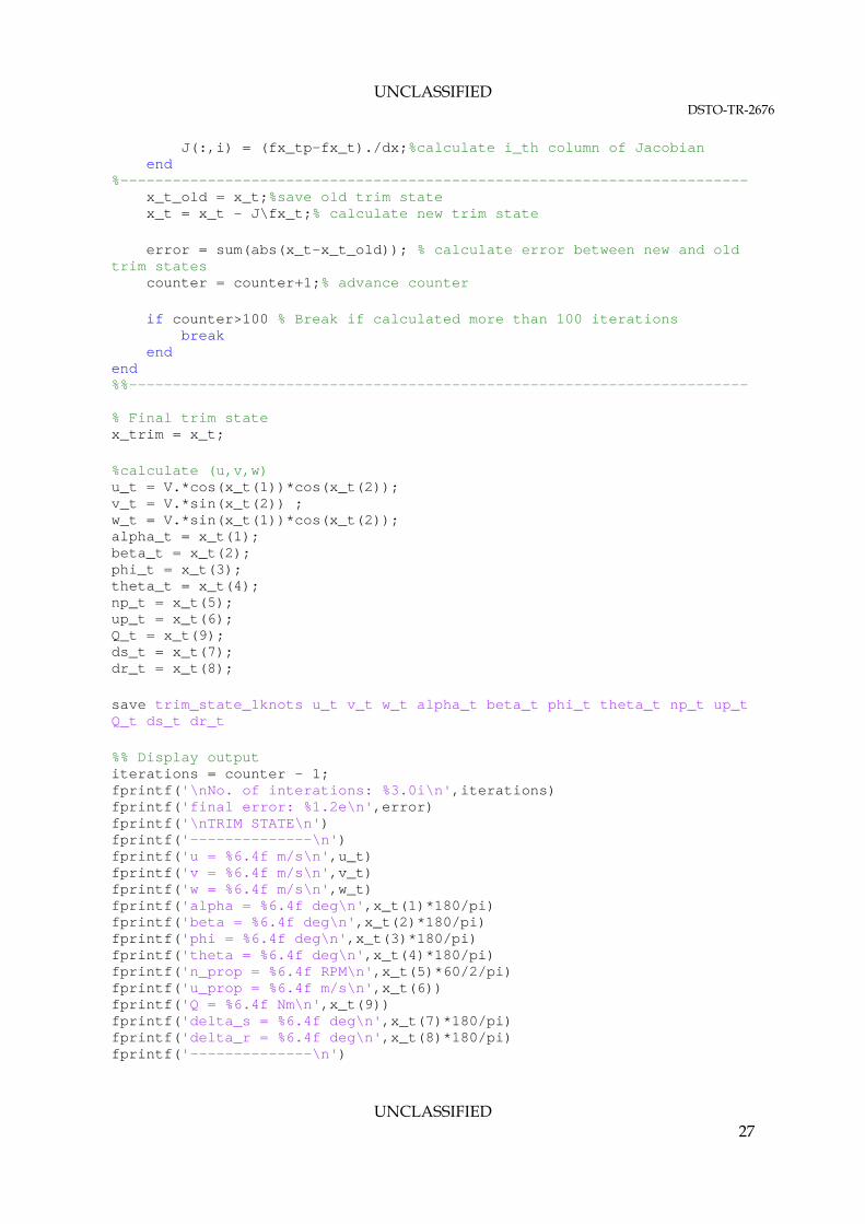
UNCLASSIFIED DSTO-TR-2676
J(:,i) = (fx_tp-fx_t)./dx;%calculate i_th column of Jacobian end %------------------------------------------------------------------------ x_t_old = x_t;%save old trim state x_t = x_t - J\fx_t;% calculate new trim state error = sum(abs(x_t-x_t_old)); % calculate error between new and old trim states counter = counter+1;% advance counter if counter>100 % Break if calculated more than 100 iterations break end end %%----------------------------------------------------------------------- % Final trim state x_trim = x_t; %calculate (u,v,w) u_t = V.*cos(x_t(1))*cos(x_t(2)); v_t = V.*sin(x_t(2)) ; w_t = V.*sin(x_t(1))*cos(x_t(2)); alpha_t = x_t(1); beta_t = x_t(2); phi_t = x_t(3); theta_t = x_t(4); np_t = x_t(5); up_t = x_t(6) ;Q_t = x_t(9); ds_t = x_t(7); dr_t = x_t(8); save trim_state_1knots u_t v_t w_t alpha_t beta_t phi_t theta_t np_t up_t Q_t ds_t dr_t %% Display output iterations = counter - 1; fprintf('\nNo. of interations: %3.0i\n',iterations) fprintf('final error: %1.2e\n',error) fprintf('\nTRIM STATE\n') fprintf('--------------\n') fprintf('u = %6.4f m/s\n',u_t) fprintf('v = %6.4f m/s\n',v_t) fprintf('w = %6.4f m/s\n',w_t) fprintf('alpha = %6.4f deg\n',x_t(1)*180/pi) fprintf('beta = %6.4f deg\n',x_t(2)*180/pi) fprintf('phi = %6.4f deg\n',x_t(3)*180/pi) fprintf('theta = %6.4f deg\n',x_t(4)*180/pi) fprintf('n_prop = %6.4f RPM\n',x_t(5)*60/2/pi) fprintf('u_prop = %6.4f m/s\n',x_t(6)) fprintf('Q = %6.4f Nm\n',x_t(9)) fprintf('delta_s = %6.4f deg\n',x_t(7)*180/pi) fprintf('delta_r = %6.4f deg\n',x_t(8)*180/pi) fprintf('--------------\n')
UNCLASSIFIED 27
UNCLASSIFIED DSTO-TR-2576
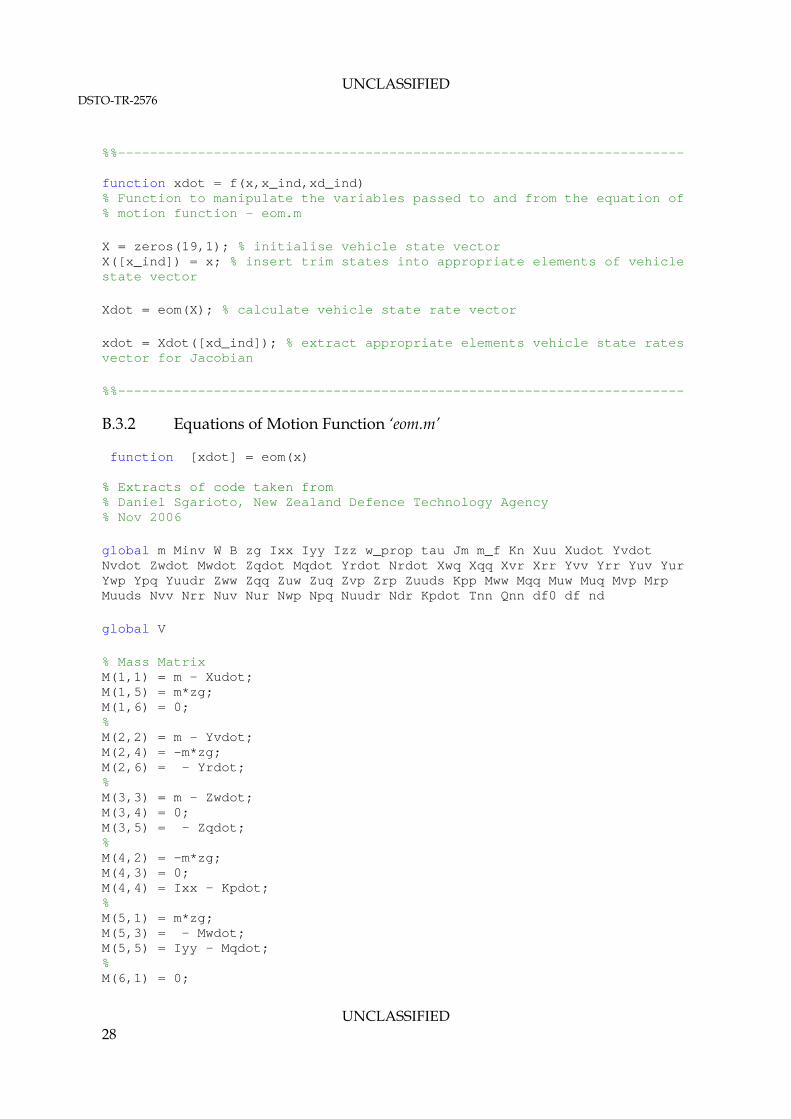
%%----------------------------------------------------------------------- function xdot = f(x,x_ind,xd_ind) % Function to manipulate the variables passed to and from the equation of % motion function - eom.m X = zeros(19,1); % initialise vehicle state vector X([x_ind]) = x; % insert trim states into appropriate elements of vehicle state vector Xdot = eom(X); % calculate vehicle state rate vector xdot = Xdot([xd_ind]); % extract appropriate elements vehicle state rates vector for Jacobian %%-----------------------------------------------------------------------
B.3.2 Equations of Motion Function ‘eom.m’
function [xdot] = eom(x) % Extracts of code taken from % Daniel Sgarioto, New Zealand Defence Technology Agency % Nov 2006 global m Minv W B zg Ixx Iyy Izz w_prop tau Jm m_f Kn Xuu Xudot Yvdot Nvdot Zwdot Mwdot Zqdot Mqdot Yrdot Nrdot Xwq Xqq Xvr Xrr Yvv Yrr Yuv Yur Ywp Ypq Yuudr Zww Zqq Zuw Zuq Zvp Zrp Zuuds Kpp Mww Mqq Muw Muq Mvp Mrp Muuds Nvv Nrr Nuv Nur Nwp Npq Nuudr Ndr Kpdot Tnn Qnn df0 df nd global V % Mass Matrix M(1,1) = m - Xudot; M(1,5) = m*zg; M(1,6) = 0; % M(2,2) = m - Yvdot; M(2,4) = -m*zg; M(2,6) = - Yrdot; % M(3,3) = m - Zwdot; M(3,4) = 0; M(3,5) = - Zqdot; % M(4,2) = -m*zg; M(4,3) = 0; M(4,4) = Ixx - Kpdot; % M(5,1) = m*zg; M(5,3) = - Mwdot; M(5,5) = Iyy - Mqdot; % M(6,1) = 0;
UNCLASSIFIED 28
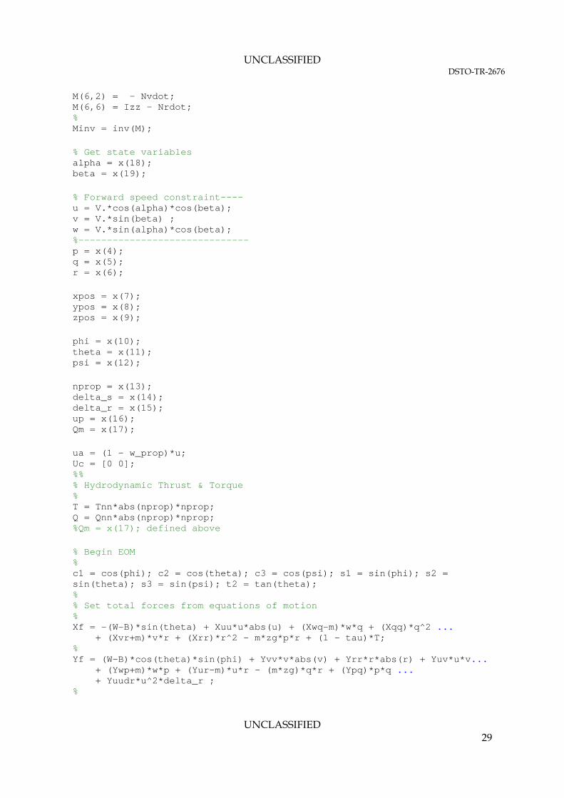
UNCLASSIFIED DSTO-TR-2676
M(6,2) = - Nvdot; M(6,6) = Izz - Nrdot; % Minv = inv(M); % Get state variables alpha = x(18); beta = x(19); % Forward speed constraint---- u = V.*cos(alpha)*cos(beta); v = V.*sin(beta) ; w = V.*sin(alpha)*cos(beta); %------------------------------ p = x(4); q = x(5); r = x(6); xpos = x(7); ypos = x(8); zpos = x(9); phi = x(10); theta = x(11); psi = x(12); nprop = x(13); delta_s = x(14); delta_r = x(15); up = x(16); Qm = x(17); ua = (1 - w_prop)*u; Uc = [0 0]; %% % Hydrodynamic Thrust & Torque % T = Tnn*abs(nprop)*nprop; Q = Qnn*abs(nprop)*nprop; %Qm = x(17); defined above % Begin EOM % c1 = cos(phi); c2 = cos(theta); c3 = cos(psi); s1 = sin(phi); s2 = sin(theta); s3 = sin(psi); t2 = tan(theta); % % Set total forces from equations of motion % Xf = -(W-B)*sin(theta) + Xuu*u*abs(u) + (Xwq-m)*w*q + (Xqq)*q^2 ... + (Xvr+m)*v*r + (Xrr)*r^2 - m*zg*p*r + (1 - tau)*T; % Yf = (W-B)*cos(theta)*sin(phi) + Yvv*v*abs(v) + Yrr*r*abs(r) + Yuv*u*v... + (Ywp+m)*w*p + (Yur-m)*u*r - (m*zg)*q*r + (Ypq)*p*q ... + Yuudr*u^2*delta_r ; %
UNCLASSIFIED 29
UNCLASSIFIED DSTO-TR-2576
Zf = (W-B)*cos(theta)*cos(phi) + Zww*w*abs(w) + Zqq*q*abs(q)+ Zuw*u*w ... + (Zuq+m)*u*q + (Zvp-m)*v*p + (m*zg)*p^2 + (m*zg)*q^2 ... + (Zrp)*r*p + Zuuds*u^2*delta_s ; % Kf = - (zg*W)*cos(theta)*sin(phi) ... + Kpp*p*abs(p) - (Izz-Iyy)*q*r - (m*zg)*w*p + (m*zg)*u*r + Q; % Mf = -(zg*W)*sin(theta) + Mww*w*abs(w) ... + Mqq*q*abs(q) + (Mrp - (Ixx-Izz))*r*p + (m*zg)*v*r - (m*zg)*w*q ... + (Muq)*u*q + Muw*u*w + (Mvp)*v*p ... + Muuds*u^2*delta_s ; % Nf = Nvv*v*abs(v) + Nrr*r*abs(r) + Nuv*u*v ... + (Npq - (Iyy-Ixx))*p*q + (Nwp)*w*p + (Nur)*u*r ... + Nuudr*u^2*delta_r ; % FORCES = [Xf Yf Zf Kf Mf Nf]' ; % xdot = ... [Minv(1,1)*Xf+Minv(1,2)*Yf+Minv(1,3)*Zf+Minv(1,4)*Kf+Minv(1,5)*Mf+Minv(1,6)*Nf Minv(2,1)*Xf+Minv(2,2)*Yf+Minv(2,3)*Zf+Minv(2,4)*Kf+Minv(2,5)*Mf+Minv(2,6)*Nf Minv(3,1)*Xf+Minv(3,2)*Yf+Minv(3,3)*Zf+Minv(3,4)*Kf+Minv(3,5)*Mf+Minv(3,6)*Nf Minv(4,1)*Xf+Minv(4,2)*Yf+Minv(4,3)*Zf+Minv(4,4)*Kf+Minv(4,5)*Mf+Minv(4,6)*Nf Minv(5,1)*Xf+Minv(5,2)*Yf+Minv(5,3)*Zf+Minv(5,4)*Kf+Minv(5,5)*Mf+Minv(5,6)*Nf Minv(6,1)*Xf+Minv(6,2)*Yf+Minv(6,3)*Zf+Minv(6,4)*Kf+Minv(6,5)*Mf+Minv(6,6)*Nf c3*c2*u + (c3*s2*s1-s3*c1)*v + (s3*s1+c3*c1*s2)*w + Uc(1) s3*c2*u + (c1*c3+s1*s2*s3)*v + (c1*s2*s3-c3*s1)*w + Uc(2) -s2*u + c2*s1*v + c1*c2*w p + s1*t2*q + c1*t2*r c1*q - s1*r s1/c2*q + c1/c2*r] ; % xdot(13,1) = (1/Jm)*(Qm - Q - (Kn*nprop)); % xdot(14,1) = (1/m_f)*(T - df0*up - df*abs(up)*(up - ua)); % ydotV = xdot(1,1)*cos(alpha)*cos(beta) + xdot(2,1)*sin(beta) + xdot(3,1)*sin(alpha)*cos(beta); % ydotA = (xdot(3,1)*cos(alpha) - xdot(1,1)*sin(alpha))/(V*cos(beta)); % ydotB = (1/V)*(-xdot(1,1)*cos(alpha)*sin(beta) + xdot(2,1)*cos(beta) - xdot(3,1)*sin(alpha)*sin(beta)); % xdot(15:17,1) = [ydotV ydotA ydotB];
UNCLASSIFIED 30
UNCLASSIFIED DSTO-TR-2676
B.3.3 Hydrodynamics Coefficients script file ‘coeffs.m’
% REMUS Hydrodynamic Coefficients % Daniel Sgarioto, DTA % Nov 2006 global V scale % Vehicle Parameters % U0=V; m = 30.48; g = 9.81; % W = m*g; B = W + (0.75*4.44822162); L = 1.3327; % zg = 0.0196; % Ixx = 0.177; Iyy = 3.45; Izz = 3.45; % cdu = 0.2; rho = 1030; Af = 0.0285; d = 0.191; xcp = 0.321; Cydb = 1.2; % mq = 0.3; % cL_alpha = 3.12; Sfin = 0.00665; xfin = -0.6827; % gamma = 1; a_prop = 0.25; w_prop = 0.2; tau = 0.1; Jm = 1; % l_prop = 0.8*0.0254; d_prop = 5.5*0.0254; A_prop = (pi/4)*(d_prop^2); m_f = gamma*rho*A_prop*l_prop; % Kn = 0.5; % % Most are Prestero's estimates, but revised values of some linear % coefficients are due to Fodrea. Thruster coeffs based on results reported by Allen et al. % Xwq= -35.5; Xqq= -1.93 ;Xvr= 35.5;
UNCLASSIFIED 31
UNCLASSIFIED DSTO-TR-2576
Xrr= -1.93; Yvv= -1310.0; Yrr= 0.632; Yuv= -28.6 ;Yur= 5.22; Ywp= 35.5; Ypq= 1.93; Yuudr= 9.64; Zww= -1310.0; Zqq= -0.632 ;Zuw= -28.6; Zuq= -5.22; Zvp= -35.5 ;Zrp= 1.93; Zuuds= -9.64; Kpp= -0.130; Mww= 3.18; Mqq= -188; Muw= 24.0; Muq= -2.0; Mvp= -1.93; Mrp= 4.86; Muuds= -6.15; Nvv= -3.18; Nrr= -94.0; Nuv= -24.0; Nur= -2.0; Nwp= -1.93; Npq= -4.86; Nuudr= -6.15*scale; Kpdot= -0.0704; % Xuu = -0.5*rho*cdu*Af; Xu = -rho*cdu*Af*U0; % % Added Mass Coeffs Xudot= -0.93; % Yvdot= -35.5; Yrdot= 1.93; % Zwdot= -35.5; Zqdot= -1.93; % Mwdot= -1.93; Mqdot= -4.88; % Nvdot= 1.93; Nrdot= -4.88; % % Added Mass Terms % Zwc = -15.7; Zqc = 0.12; % Mwc = -0.403; Mqc = -2.16;
UNCLASSIFIED 32
UNCLASSIFIED DSTO-TR-2676
% % Added Mass Coupling Terms Xqa = Zqdot*mq; Zqa = -Xudot*U0; Mwa = -(Zwdot - Xudot)*U0; Mqa = -Zqdot*U0; % % Body Lift Contribution % Zwl = -0.5*rho*(d^2)*Cydb*U0; % Mwl = -0.5*rho*(d^2)*Cydb*xcp*U0; % % Fin Contribution % Zwf = -0.5*rho*cL_alpha*Sfin*U0; Zqf = 0.5*rho*cL_alpha*Sfin*xfin*U0; % Mwf = 0.5*rho*cL_alpha*Sfin*xfin*U0; Mqf = -0.5*rho*cL_alpha*Sfin*(xfin^2)*U0; % % Dive Plane Coeffs Zw = Zwc + Zwl + Zwf; Zq = 2.2; % Mw = -9.3; Mq = Mqc +Mqa +Mqf; % % Steering Coeffs Yv = Zw; Yr = 2.2; % Nv = -4.47; Nr = Mq; % % Control Surface Coeffs Zds = -rho*cL_alpha*Sfin*(U0^2); Mds = rho*cL_alpha*Sfin*xfin*(U0^2); % Ydr = -Zds/3.5 ;Ndr = Mds/3.5; % % Thruster Coeffs Tnn = 6.279e-004; Tnu = 0; % Qnn = -1.121e-005; Qnu = 0; % Tnu0 = (1/(a_prop + 1))*Tnu; Qnu0 = (1/(a_prop + 1))*Qnu; % df0 = (-Xu)/((1 - tau)*(1 + a_prop)*(1 - w_prop)); df = (-Xuu)/((1 - tau)*(1 + a_prop)*a_prop*((1 - w_prop)^2)); %
UNCLASSIFIED 33
UNCLASSIFIED DSTO-TR-2576
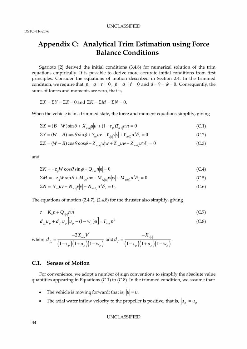
Appendix C: Analytical Trim Estimation using Force Balance Conditions
Sgarioto [2] derived the initial conditions (3.4.8) for numerical solution of the trim equations empirically. It is possible to derive more accurate initial conditions from first principles. Consider the equations of motion described in Section 2.4. In the trimmed condition, we require that 0 rqp , 0 rqp and .0 wvu Consequently, the sums of forces and moments are zero, that is, and 0 ZYX .0 NMK When the vehicle is in a trimmed state, the force and moment equations simplify, giving 0)1(sin)( nnTuuXWBX nnpuu (C.1)
0sincos)( 2 ruuvvuv uYvvYuvYBWYr
(C.2)
0coscos)( 2 suuuwww uZuwZwwZBWZs (C.3)
and 0sincos nnQWzK nng (C.4)
0sin 2 suuwwuwg uMwwMuwMWzMs (C.5)
.02 ruuvvuv uNvvNuvNNr
(C.6)
The equations of motion (2.4.7), (2.4.8) for the thruster also simplify, giving nnQnK nnn (C.7)
2)1(0
nTuwuudud nnpppfpf (C.8)
where 0
2
1 1 1
u u
f
p p
X Vd
a w
p
and 1 1 1
u u
f
p p
Xd
a w p
.
C.1. Senses of Motion
For convenience, we adopt a number of sign conventions to simplify the absolute value quantities appearing in Equations (C.1) to (C.8). In the trimmed condition, we assume that:
The vehicle is moving forward; that is, .uu
The axial water inflow velocity to the propeller is positive; that is, .pp uu
UNCLASSIFIED 34
UNCLASSIFIED DSTO-TR-2676
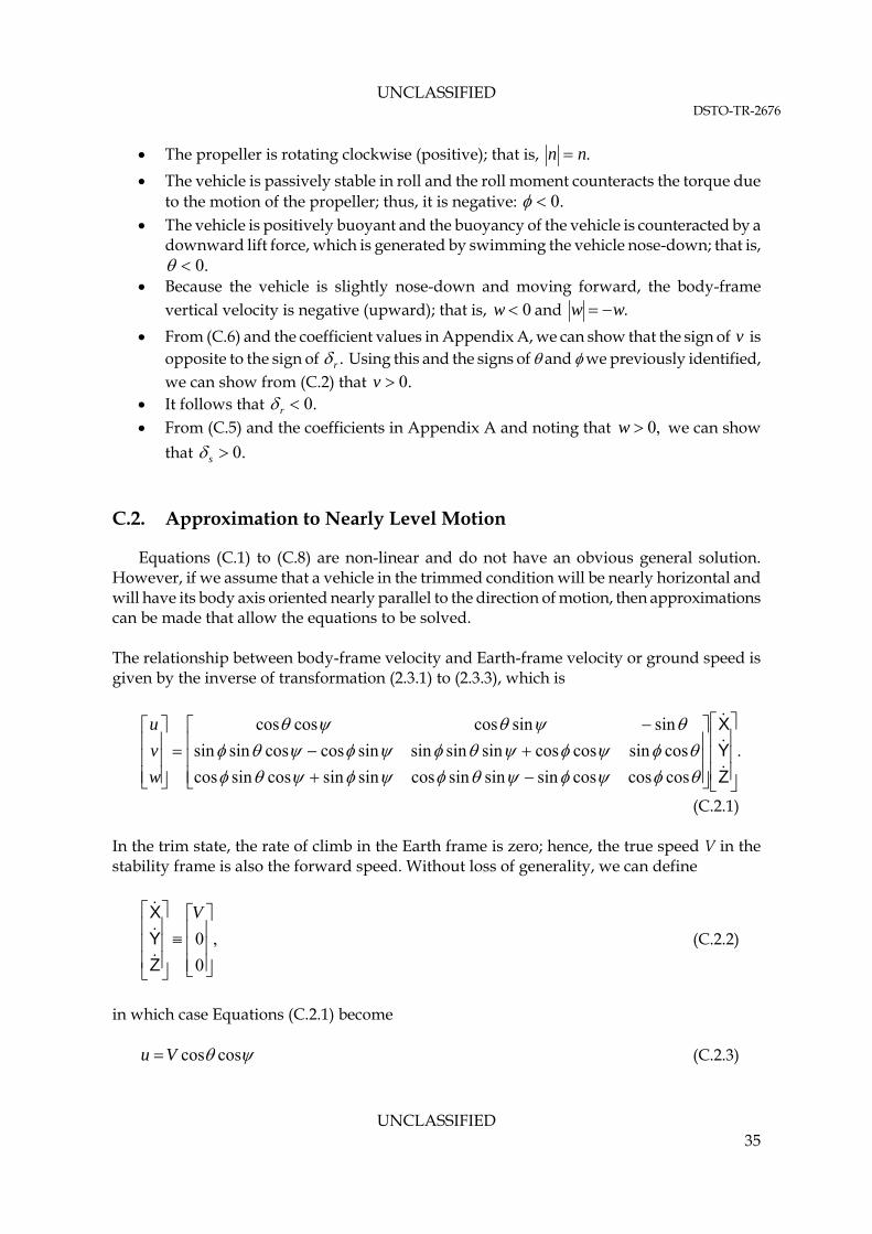
The propeller is rotating clockwise (positive); that is, .nn
The vehicle is passively stable in roll and the roll moment counteracts the torque due to the motion of the propeller; thus, it is negative: .0
The vehicle is positively buoyant and the buoyancy of the vehicle is counteracted by a downward lift force, which is generated by swimming the vehicle nose-down; that is,
.0 Because the vehicle is slightly nose-down and moving forward, the body-frame
vertical velocity is negative (upward); that is, 0w and .ww
From (C.6) and the coefficient values in Appendix A, we can show that the sign of v is opposite to the sign of .r Using this and the signs of and we previously identified, we can show from (C.2) that .0v
It follows that .0r From (C.5) and the coefficients in Appendix A and noting that ,0w we can show
that .0s
C.2. Approximation to Nearly Level Motion
Equations (C.1) to (C.8) are non-linear and do not have an obvious general solution. However, if we assume that a vehicle in the trimmed condition will be nearly horizontal and will have its body axis oriented nearly parallel to the direction of motion, then approximations can be made that allow the equations to be solved. The relationship between body-frame velocity and Earth-frame velocity or ground speed is given by the inverse of transformation (2.3.1) to (2.3.3), which is
.
coscoscossinsinsincossinsincossincos
cossincoscossinsinsinsincoscossinsin
sinsincoscoscos
Z
Y
X
w
v
u
(C.2.1) In the trim state, the rate of climb in the Earth frame is zero; hence, the true speed V in the stability frame is also the forward speed. Without loss of generality, we can define
(C.2.2) ,
0
0
V
Z
Y
X
in which case Equations (C.2.1) become coscosVu (C.2.3)
UNCLASSIFIED 35
UNCLASSIFIED DSTO-TR-2576
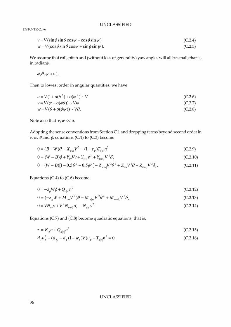
)sincoscossin(sin Vv (C.2.4) ).sinsincossin(cos Vw (C.2.5) We assume that roll, pitch and (without loss of generality) yaw angles will all be small; that is, in radians, .1,, Then to lowest order in angular quantities, we have (C.2.6) VooVu ~)()(1( 22 VoVv ~))(( (C.2.7) .~))(( VoVw (C.2.8) Note also that ., uwv Adopting the sense conventions from Section C.1 and dropping terms beyond second order in v, w, and , equations (C.1) to (C.3) become 22 )1()(0 nTVXWB nnpuu (C.2.9)
ruuvvuv VYvYVvYBWr
22)(0 (C.2.10)
.]5.05.01)[(0 222222suuuwww VZVZVZBW
s (C.2.11)
Equations (C.4) to (C.6) become 20 nQWz nng (C.2.12)
suuwwuwg VMVMVMWzs
2222 )(0 (C.2.13)
.0 22 vNNVvVN vvruuuv r (C.2.14)
Equations (C.7) and (C.8) become quadratic equations, that is, 2nQnK nnn (C.2.15)
.0))1(( 22
0 nTuVwddud nnppffpf (C.2.16)
UNCLASSIFIED 36
UNCLASSIFIED DSTO-TR-2676
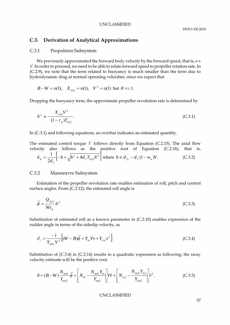
C.3. Derivation of Analytical Approximations
C.3.1 Propulsion Subsystem
We previously approximated the forward body velocity by the forward speed, that is, u V. In order to proceed, we need to be able to relate forward speed to propeller rotation rate. In (C.2.9), we note that the term related to buoyancy is much smaller than the term due to hydrodynamic drag at normal operating velocities, since we expect that .1but )1(),1(),1( 2 oVoXoWB uu
Dropping the buoyancy term, the approximate propeller revolution rate is determined by
.)1(
2
2
nnp
uu
T
VXn
(C.3.1)
In (C.3.1) and following equations, an overbar indicates an estimated quantity. The estimated control torque follows directly from Equation (C.2.15). The axial flow velocity also follows as the positive root of Equation (C.2.16), that is,
.)1( where42
10
22 VwddbnTdbbd
u pffnnff
p (C.3.2)
C.3.2 Manoeuvre Subsystem
Estimation of the propeller revolution rate enables estimation of roll, pitch and control surface angles. From (C.2.12), the estimated roll angle is
.2nWz
Q
g
nn (C.3.3)
Substitution of estimated roll as a known parameter in (C.2.10) enables expression of the rudder angle in terms of the sideslip velocity, as
.)(1 2
2vYVvYBW
VY vvuv
uu
r
r
(C.3.4)
Substitution of (C.3.4) in (C.2.14) results in a quadratic expression as following; the sway velocity estimate will be the positive root.
.)(0 2vY
YNNvV
Y
YNN
Y
NWB
r
r
r
r
r
r
uu
vvuu
vvuu
uvuuuv
uu
uu
(C.3.5)
UNCLASSIFIED 37
UNCLASSIFIED DSTO-TR-2576
The rudder angle follows from (C.2.14), as
.1 2
2vVNvN
VN uvvvuu
r
r
(C.3.6)
Similarly, substitution of the estimated roll in (C.2.11) allows expression of the elevator angle in terms of pitch, as
.)(5.05.01)(1 2222
2
VZWBVZBWVZ wwuw
uus
s
(C.3.7)
Substituting (C.3.7) in (C.2.13) yields a quadratic expression for the pitch estimate, as
.)(5.0
5.01)(0
222
222
WBZ
MV
Z
ZMVM
VMWzVZ
MZBW
Z
M
s
s
s
s
s
s
s
s
uu
uu
uu
wwuu
ww
uwguu
uuuw
uu
uu
(C.3.8)
The pitch estimate is the negative root of the quadratic. The estimated elevator angle follows directly from (C.3.7). Together, the equations in this section approximate the state of the vehicle in a trimmed condition. C.4. Comparison of Numerical and Analytical Trim Estimates
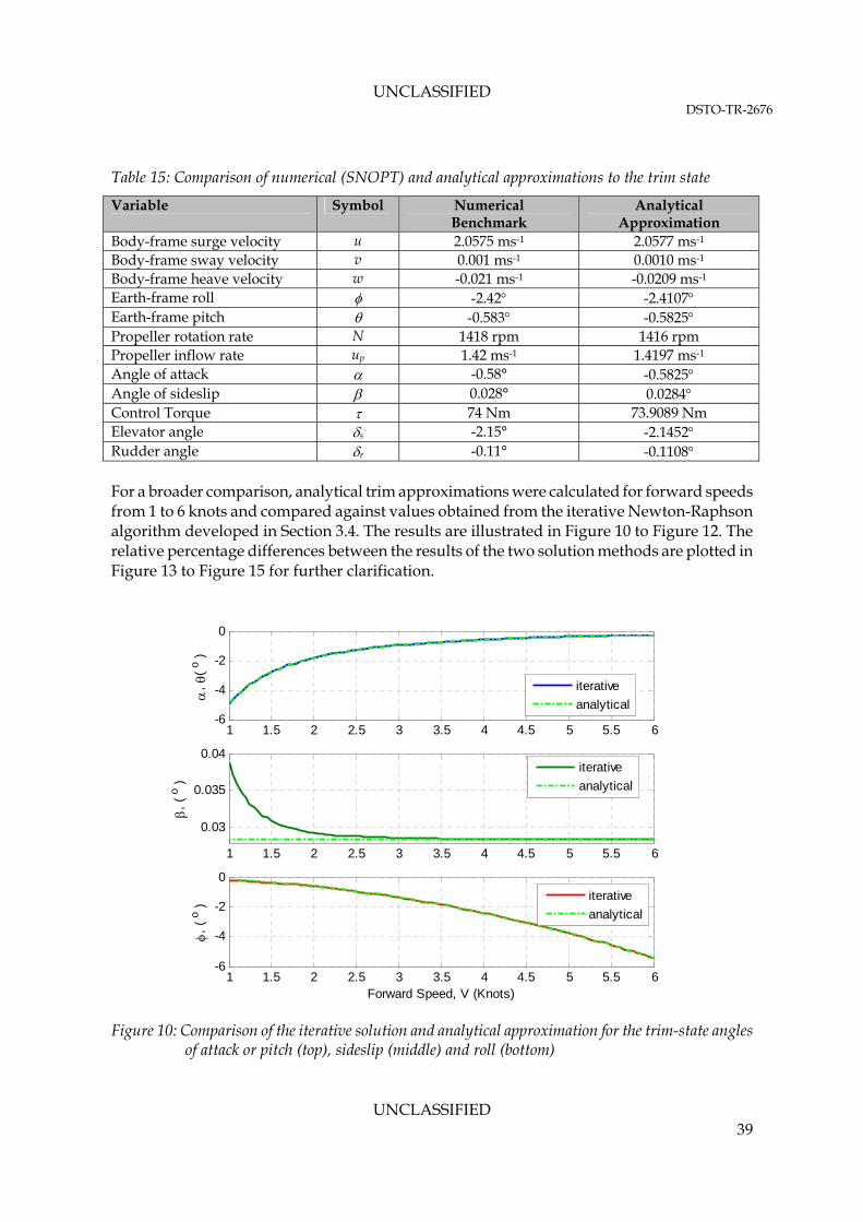
Physical intuition suggests that the accuracy of equations (C.3.1) to (C.3.8) should improve with increasing forward speed. In order to compare the present approach to estimating the trim conditions with the iterative approach adopted in Section 3.4, we substitute the coefficient values from Appendix A into the equations and evaluate them. In order to compare with the case-study of Sgarioto [2], we set V = 4 knots and take the buoyancy force as 0.75 pounds weight, that is, 0.75 × 0.45 × 9.81 = 3.3 N. The results are shown in Table 15. By inspection, the state variables estimated with the analytical approximation are mostly in agreement with the ‘benchmark’ values estimated by Sgarioto or using the Newton-Raphson method described in Section 3.4, to two or three significant figures.
UNCLASSIFIED 38
UNCLASSIFIED DSTO-TR-2676
Table 15: Comparison of numerical (SNOPT) and analytical approximations to the trim state
Variable Symbol Numerical Benchmark
Analytical Approximation
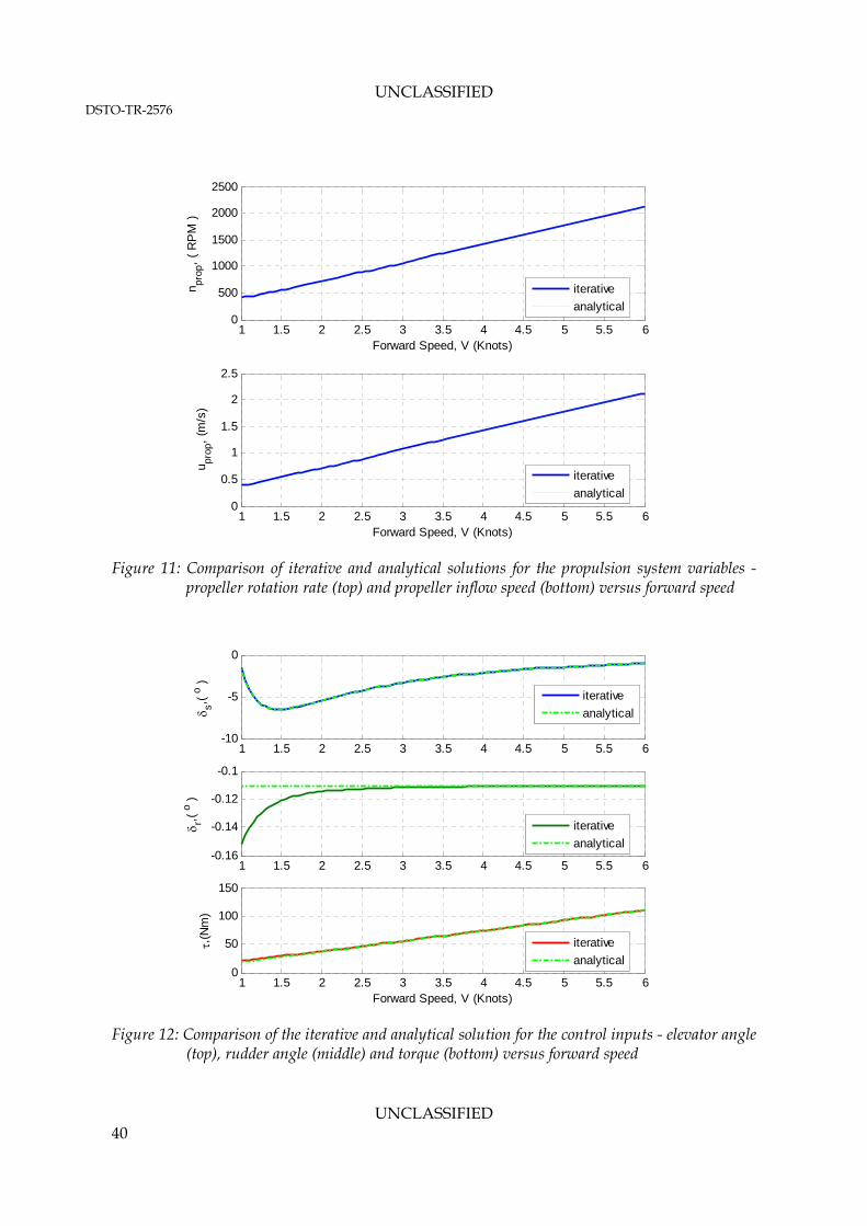
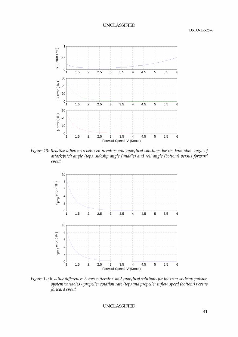
Body-frame surge velocity u 2.0575 ms-1 2.0577 ms-1 Body-frame sway velocity v 0.001 ms-1 0.0010 ms-1 Body-frame heave velocity w -0.021 ms-1 -0.0209 ms-1 Earth-frame roll -2.42 -2.4107 Earth-frame pitch -0.583 -0.5825 Propeller rotation rate N 1418 rpm 1416 rpm Propeller inflow rate up 1.42 ms-1 1.4197 ms-1 Angle of attack -0.58° -0.5825 Angle of sideslip 0.028° 0.0284 Control Torque 74 Nm 73.9089 Nm Elevator angle s -2.15° -2.1452 Rudder angle r -0.11° -0.1108 For a broader comparison, analytical trim approximations were calculated for forward speeds from 1 to 6 knots and compared against values obtained from the iterative Newton-Raphson algorithm developed in Section 3.4. The results are illustrated in Figure 10 to Figure 12. The relative percentage differences between the results of the two solution methods are plotted in Figure 13 to Figure 15 for further clarification.
1 1.5 2 2.5 3 3.5 4 4.5 5 5.5 6-6
-4
-2
0
, (
o )
1 1.5 2 2.5 3 3.5 4 4.5 5 5.5 6
0.03
0.035
0.04
, (
o )
1 1.5 2 2.5 3 3.5 4 4.5 5 5.5 6-6
-4
-2
0
, (
o )
Forward Speed, V (Knots)
iterative
analytical
iterative
analytical
iterative
analytical
Figure 10: Comparison of the iterative solution and analytical approximation for the trim-state angles
of attack or pitch (top), sideslip (middle) and roll (bottom)
UNCLASSIFIED 39
UNCLASSIFIED DSTO-TR-2576
1 1.5 2 2.5 3 3.5 4 4.5 5 5.5 60
500
1000
1500
2000
2500
Forward Speed, V (Knots)
n prop
, (
RP
M )
1 1.5 2 2.5 3 3.5 4 4.5 5 5.5 60
0.5
1
1.5
2
2.5
Forward Speed, V (Knots)
upr
op,
(m/s
)
iterative
analytical
iterative
analytical
Figure 11: Comparison of iterative and analytical solutions for the propulsion system variables -
propeller rotation rate (top) and propeller inflow speed (bottom) versus forward speed
1 1.5 2 2.5 3 3.5 4 4.5 5 5.5 6-10
-5
0
s,(
o )
1 1.5 2 2.5 3 3.5 4 4.5 5 5.5 6-0.16
-0.14
-0.12
-0.1
r,(
o )
1 1.5 2 2.5 3 3.5 4 4.5 5 5.5 60
50
100
150
,(N
m)
Forward Speed, V (Knots)
iterative
analytical
iterative
analytical
iterative
analytical
Figure 12: Comparison of the iterative and analytical solution for the control inputs - elevator angle
(top), rudder angle (middle) and torque (bottom) versus forward speed
UNCLASSIFIED 40
UNCLASSIFIED DSTO-TR-2676
1 1.5 2 2.5 3 3.5 4 4.5 5 5.5 60
0.5
1
,
err
or (
% )
1 1.5 2 2.5 3 3.5 4 4.5 5 5.5 60
10
20
30
er
ror
( %
)
1 1.5 2 2.5 3 3.5 4 4.5 5 5.5 60
10
20
30
er
ror
( %
)
Forward Speed, V (Knots)
Figure 13: Relative differences between iterative and analytical solutions for the trim-state angle of attack/pitch angle (top), sideslip angle (middle) and roll angle (bottom) versus forward speed
1 1.5 2 2.5 3 3.5 4 4.5 5 5.5 60
2
4
6
8
10
n prop
err
or (
% )
1 1.5 2 2.5 3 3.5 4 4.5 5 5.5 60
2
4
6
8
10
Forward Speed, V (Knots)
u prop
err
or (
% )
Figure 14: Relative differences between iterative and analytical solutions for the trim-state propulsion
system variables - propeller rotation rate (top) and propeller inflow speed (bottom) versus forward speed
UNCLASSIFIED 41
UNCLASSIFIED DSTO-TR-2576
1 1.5 2 2.5 3 3.5 4 4.5 5 5.5 6-4
-2
0
2
s e
rror
( %
)
1 1.5 2 2.5 3 3.5 4 4.5 5 5.5 60
10
20
30
r e
rror
( %
)
1 1.5 2 2.5 3 3.5 4 4.5 5 5.5 60
5
10
15
er
ror
( %
)
Forward Speed, V (Knots)
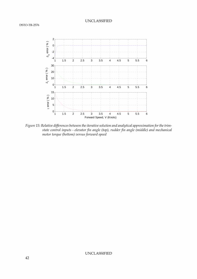
Figure 15: Relative differences between the iterative solution and analytical approximation for the trim-state control inputs - elevator fin angle (top), rudder fin angle (middle) and mechanical motor torque (bottom) versus forward speed
UNCLASSIFIED 42
UNCLASSIFIED DSTO-TR-2676
Appendix D: Convergence Sensitivity Analysis
In order to test the robustness of the numerical trim-estimation algorithm, a sensitivity analysis of the convergence behaviour was conducted with respect to the values of the hydrodynamic coefficients. The robustness of the algorithm to different vehicle models was tested by altering the values of five primary hydrodynamic coefficients: ,uwM ,
suuM ,ruuN uuX and . This set
consists of coefficients which Sgarioto previously identified as having a significant impact on the longitudinal (x-z plane) stability of the REMUS model [2]. Each of the parameters is also sensitive to the physical dimensions of the vehicle.
uwZ
A parametric analysis was performed by varying each of the five coefficients individually. This was done by running the trim algorithm for a forward speed of 4 knots with the value of the coefficient at 50%, 75%, 100%, 125% and 150% of the original value provided in A.1. The performance of the algorithm was compared using the number of iterations it took in each case to reach the preset error tolerance. It should be noted that, while speed of convergence has been used here as a measure of robustness, a comprehensive analysis would employ methods that consider the complete topology of the characteristic surface. It was found that all the cases resulted in convergence to a trim solution and that in most cases the same number of iterations was required to converge as for the benchmark case. In a few cases, convergence occurred after one less iteration than the benchmark. The trim variable results are summarised for each coefficient in Table 16 to Table 20 along with the corresponding number of iterations taken to reach convergence. As the values of the many trim variables did not change significantly compared to the original numerical benchmark solution, the trim variable results are listed as a percentage difference from the original solution. For example, the percentage difference in the angle of attack when the coefficient is reduced to 50% of its original value is calculated as follows:
100_%100
%50%100
differencepercent
As expected, the results show that only the variables associated with the mode of motion affected by the coefficient in question will change. For example, Table 16 shows that , a
coefficient linking the elevator’s surface deflection to the vehicle’s pitching motion significantly affects only the pitch angle (and angle of attack) and the elevator trim angle. The results from varying Zuw and Muw show similar patterns, as expected because these coefficients are related to the same modes of motion as
suuM
.suuM
UNCLASSIFIED 43
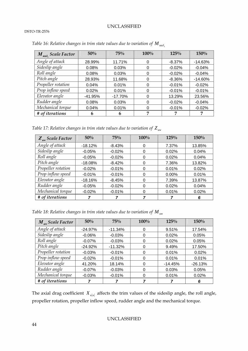
UNCLASSIFIED DSTO-TR-2576
Table 16: Relative changes in trim state values due to variation of suuM
suuδM Scale Factor 50% 75% 100% 125% 150%
Angle of attack 28.99% 11.71% 0 -8.37% -14.63% Sideslip angle 0.08% 0.03% 0 -0.02% -0.04% Roll angle 0.08% 0.03% 0 -0.02% -0.04% Pitch angle 28.93% 11.68% 0 -8.36% -14.60% Propeller rotation 0.04% 0.01% 0 -0.01% -0.02% Prop inflow speed 0.02% 0.01% 0 -0.01% -0.01% Elevator angle -41.95% -17.70% 0 13.29% 23.56% Rudder angle 0.08% 0.03% 0 -0.02% -0.04% Mechanical torque 0.04% 0.01% 0 -0.01% -0.02% # of iterations 6 6 7 7 7
Table 17: Relative changes in trim state values due to variation of uwZ
uwZ Scale Factor 50% 75% 100% 125% 150%
Angle of attack -18.12% -8.43% 0 7.37% 13.85% Sideslip angle -0.05% -0.02% 0 0.02% 0.04% Roll angle -0.05% -0.02% 0 0.02% 0.04% Pitch angle -18.08% -8.42% 0 7.36% 13.82% Propeller rotation -0.02% -0.01% 0 0.01% 0.02% Prop inflow speed -0.01% -0.01% 0 0.00% 0.01% Elevator angle -18.16% -8.45% 0 7.39% 13.87% Rudder angle -0.05% -0.02% 0 0.02% 0.04% Mechanical torque -0.02% -0.01% 0 0.01% 0.02% # of iterations 7 7 7 7 6
Table 18: Relative changes in trim state values due to variation of uwM
uwM Scale Factor 50% 75% 100% 125% 150%
Angle of attack -24.97% -11.34% 0 9.51% 17.54% Sideslip angle -0.06% -0.03% 0 0.02% 0.05% Roll angle -0.07% -0.03% 0 0.02% 0.05% Pitch angle -24.92% -11.32% 0 9.49% 17.50% Propeller rotation -0.03% -0.01% 0 0.01% 0.02% Prop inflow speed -0.02% -0.01% 0 0.01% 0.01% Elevator angle 41.20% 18.14% 0 -14.45% -26.13% Rudder angle -0.07% -0.03% 0 0.03% 0.05% Mechanical torque -0.03% -0.01% 0 0.01% 0.02% # of iterations 7 7 7 7 6
The axial drag coefficient uuX affects the trim values of the sideslip angle, the roll angle,
propeller rotation, propeller inflow speed, rudder angle and the mechanical torque.
UNCLASSIFIED 44
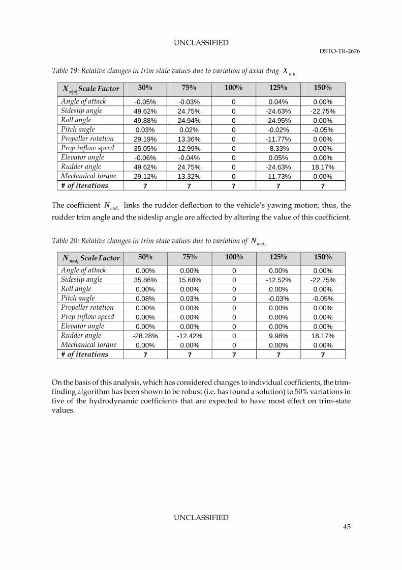
UNCLASSIFIED DSTO-TR-2676
UNCLASSIFIED 45
able 19: Relative changes in trim state values due to variation of axial drag uuXT
uuX Scale Factor 50% 75% 100% 125% 150%
Angl -0.05% -0.03% e of attack 0 0.04% 0.00% Sideslip angle 49.62% 24.75% 0 - - 24.63% 22.75%Roll angle 49.88% 24.94% 0 -24.95% 0.00% Pitch angle 0.03% 0.02% 0 -0.02% -0.05% Propeller rotation 29.19% 13.36% 0 -11.77% 0.00% Prop inflow speed 35.05% 12.99% 0 -8.33% 0.00% Elevator angle -0.06% -0.04% 0 0.05% 0.00% Rudder angle 49.62% 24.75% 0 -24.63% 18.17% Mechanical torque 29.12% 13.32% 0 -11.73% 0.00% # of iterations 7 7 7 7 7
h links the rudder de ion; thus, the
able 20: Relative changes in trim state values due to variation of
ruuN flection to the vehicle’s yawing motT e coefficient
rudder trim angle and the sideslip angle are affected by altering the value of this coefficient.
ruuN T
ruuδN Scale Factor 50% 75% 100% 125% 150%
Angle 0 0 of attack .00% .00% 0 0.00% 0.00% Sideslip angle 35.86% 15.68% -0 12.52% -22.75% Roll angle 0.00% 0.00% 0 0.00% 0.00% Pitch angle 0.08% 0.03% 0 -0.03% -0.05% Propeller rotation 0.00% 0.00% 0 0.00% 0.00% Prop inflow speed 0.00% 0.00% 0 0.00% 0.00% Elevator angle 0.00% 0.00% 0 0.00% 0.00% Rudder angle -28.28% -12.42% 0 9.98% 18.17% Mechanical torque 0.00% 0.00% 0 0.00% 0.00% # of iterations 7 7 7 7 7
n the basis of this analysis, which has considered changes to individual coefficients, the trim- Ofinding algorithm has been shown to be robust (i.e. has found a solution) to 50% variations in five of the hydrodynamic coefficients that are expected to have most effect on trim-state values.
Page classification: UNCLASSIFIED
DEFENCE SCIENCE AND TECHNOLOGY ORGANISATION
DOCUMENT CONTROL DATA 1. PRIVACY MARKING/CAVEAT (OF DOCUMENT)
2. TITLE Trim Calculation Methods for a Dynamical Model of the REMUS 100 Autonomous Underwater Vehicle
3. SECURITY CLASSIFICATION (FOR UNCLASSIFIED REPORTS THAT ARE LIMITED RELEASE USE (L) NEXT TO DOCUMENT CLASSIFICATION) Document (U) Title (U) Abstract (U)
4. AUTHOR(S) Raewyn Hall and Stuart Anstee
5. CORPORATE AUTHOR DSTO Defence Science and Technology Organisation PO Box 1500 Edinburgh South Australia 5111 Australia
6a. DSTO NUMBER DSTO-TR-2576
6b. AR NUMBER AR-015-046
6c. TYPE OF REPORT Technical Report
7. DOCUMENT DATE August 2011
8. FILE NUMBER 490-6-395
9. TASK NUMBER NAV 07/088
10. TASK SPONSOR DGMD/DGNHM/ COMMHP
11. NO. OF PAGES 45
12. NO. OF REFERENCES 4
13. DSTO Publications cRepository http://dspace.dsto.defence.gov.au/dspace/
14. RELEASE AUTHORITY Chief, Maritime Operations Division
15. SECONDARY RELEASE STATEMENT OF THIS DOCUMENT
Approved for public release OVERSEAS ENQUIRIES OUTSIDE STATED LIMITATIONS SHOULD BE REFERRED THROUGH DOCUMENT EXCHANGE, PO BOX 1500, EDINBURGH, SA 5111 16. DELIBERATE ANNOUNCEMENT No Limitations 17. CITATION IN OTHER DOCUMENTS Yes 18. DSTO RESEARCH LIBRARY THESAURUS http://web-vic.dsto.defence.gov.au/workareas/library/resources/dsto_thesaurus.shtml Autonomous Vehicles, Control Systems, Stability, Dynamic Characteristics 19. ABSTRACT The calculations given in this work demonstrate that the trimmed state for a dynamical model of the REMUS 100 autonomous underwater vehicle is readily found using a numerical zero-finding procedure based on Newton-Raphson iteration. This work also presents approximate analytical expressions for the trimmed state that can be used as a starting point for the numerical procedure. The procedure should be applicable to a range of hydrodynamic parameters corresponding to other configurations of the REMUS 100 vehicle and to similar vehicles from other vendors.
Page classification: UNCLASSIFIED
Recommended


![DCC - DMF Lighting · adfad Custom Color 13 TRIM UP 14 [Blank] N/A R Round Beveled Trim H Hyperbolic Trim S Snoot D Decorative Trim L Low Profile Decorative Trim](https://img.pdfslide.us/doc/110x75/5fd67a8e4a039075ec6b51b4/dcc-dmf-lighting-adfad-custom-color-13-trim-up-14-blank-na-r-round-beveled.jpg)