1
This is a preprint of an Article accepted for publication in Cladistics © 2012 WILLI HENNIG SOCIETY
Tree thinking, time and topology:
Comments on the interpretation of tree diagrams in
evolutionary/phylogenetic systematics
János Podani
Department of Plant Systematics, Ecology and Theoretical Biology, Institute of Biology, L.
Eötvös University and Ecology Research Group of the Hungarian Academy of Sciences,
Pázmány P. s. 1/C, H-1117 Budapest, Hungary. E-mail: [email protected]
Running title: Tree thinking, time and topology in systematic biology
2
Abstract: This paper presents a graph theoretical overview of tree diagrams applied
extensively in systematic biology. Simple evolutionary models involving three speciation
processes (splitting, budding and anagenesis) are used for evaluating the ability of different
rooted trees to demonstrate temporal and ancestor-descendant relationships within- or among
species. On this basis, they are classified into four types: 1) diachronous trees depict
evolutionary history faithfully because the order of nodes along any path agrees with the
temporal sequence of respective populations or species, 2) achronous trees show ancestor-
descendant relationships for species or higher taxa such that the time aspect is disregarded, 3)
synchronous trees attempt to reveal evolutionary pathways and/or distributional pattern of
apomorphic characters for organisms living at the same point of time, and 4) asynchronous
trees may do the same regardless the time of origin (e.g., when extant and extinct species are
evaluated together). Trees of the last two types are cladograms; the synchronous ones
emphasizing predominantly – but not exclusively – the evolutionary process within a group,
while asynchronous cladograms are usually focused on pattern and infrequently on process.
Historical comments and the examples demonstrate that each of these tree types is useful on
its own right in evolutionary biology and systematics. In practice, separation among them is
not sharp, and their features are often combined into eclectic tree forms whose interpretation
is not entirely free from problems.
3
Table of contents
Introduction 4
A false critique 5
Further examples 8
Discussion: basic tree types in evolutionary biology 11
1. Diachronous trees 11
2. Achronous trees 12
3. Synchronous trees 13
4. Asynchronous trees 15
5. Eclectic forms 17
Concluding remarks 17
References 19
Figures 1-6 23
4
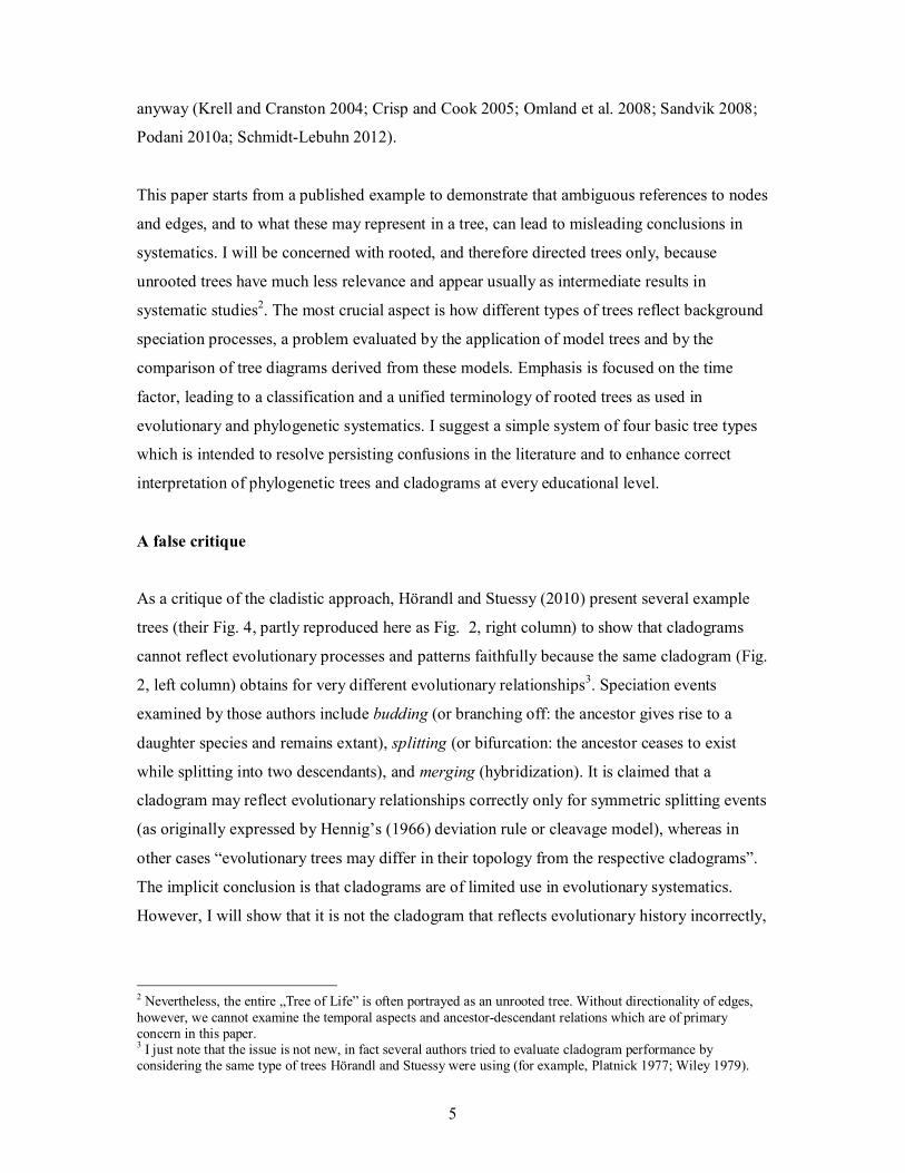
Introduction
Tree-like drawings have long been used to summarize morphological affinities or
evolutionary relationships in the organic world (O’Hara 1992; Panchen 1992; Ragan 2009;
Kutschera 2011; Tassy 2011) demonstrating that, for many biologists, practically any
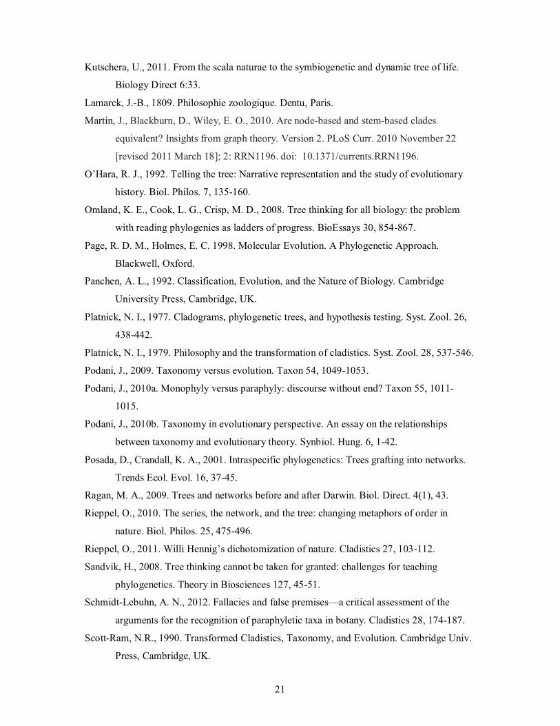
branched pattern may be conceived as a tree. In particular, figures composed of a “trunk” and
several “branches” are commonly used to illustrate evolutionary history and are therefore
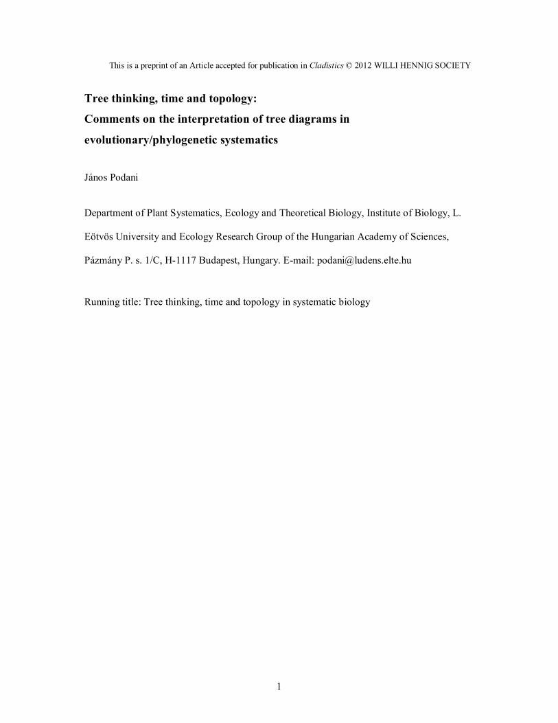
called phylogenetic trees (Fig. 1.a-b). In mathematics, however, trees are precisely defined in
graph theoretical terms as being a collection of nodes (or vertices) and a set of edges
connecting pairs of nodes such that there is only one path between any two nodes (in other
words, there is no circle in the graph, Yellen and Gross 2005). In general, the nodes represent
objects (or sets of objects) whereas the edges correspond to relations between objects (Fig.
1.c). Thus, the diagrams of Fig. 1.a-b in fact do not qualify as mathematical trees, just like
hundreds of other published drawings in which 1) the exact meaning of nodes and edges is
often forgotten, or 2) these two constituents of the graph are not even distinguished from each
other. These problems are especially striking 1) when a tree is contrasted with a classification
to explain, for instance, the notions of monophyly, stem or crown groups, and node-based or
branch-based clades (Fig. 1.d) and also 2) when vague statements such as “branches represent
OTU’s” (Camin and Sokal 1965, p. 321) and “edges correspond to ancestors” (Hörandl and
Stuessy 2010, p. 1649) are made1. Often, distinction is drawn between “cladograms and trees”
(emphasis mine, examples in Panchen 1992) as if cladograms were something other than
mathematical trees. Loose usage of terminology in biology is unfortunate if we consider how
much mathematical sophistication is involved in contemporary phylogenetic methodology to
“reconstruct” evolutionary history. Apparently, non-mathematical tree thinking is a source of
confusions in a research area which is heavily burdened by fallacies and misinterpretations
1 As Wiley and Lieberman (2011) and Martin et al. (2010) emphasized, one source of confusion is that phylogenetic trees can be drawn in two different ways. In „node-based” trees, vertices are taxa and edges correspond to relations between them. In „stem-based trees”, however, „edges are taxa and the nodes are speciation events” (p. 86 in Wiley and Lieberman 2011, see also Martin et al. 2010). In my view, the latter type is ambiguous and ill-defined because terminal vertices in stem-based trees cannot be associated with speciation events, a point that probably escaped the attention of the authors who otherwise warned that „one cannot have an edge without both its endpoints” (Martin et al. 2010). Some confusion appears in Wiley and Lieberman’s book itself, since in their Fig. 4.1.a one edge is labeled “edge” while another as “leaf”, although the latter has been reserved for terminal vertices or tips in graph theory. Nonetheless, phylogenetic (taxon-) trees are more readily comparable with population-level evolutionary trees, cladograms and tokogenetic graphs (see footnote 5) if vertices correspond to taxa (or other entities) and edges are relations, so this convention will be followed throughout this paper.
5
anyway (Krell and Cranston 2004; Crisp and Cook 2005; Omland et al. 2008; Sandvik 2008;
Podani 2010a; Schmidt-Lebuhn 2012).
This paper starts from a published example to demonstrate that ambiguous references to nodes
and edges, and to what these may represent in a tree, can lead to misleading conclusions in
systematics. I will be concerned with rooted, and therefore directed trees only, because
unrooted trees have much less relevance and appear usually as intermediate results in
systematic studies2. The most crucial aspect is how different types of trees reflect background
speciation processes, a problem evaluated by the application of model trees and by the
comparison of tree diagrams derived from these models. Emphasis is focused on the time
factor, leading to a classification and a unified terminology of rooted trees as used in
evolutionary and phylogenetic systematics. I suggest a simple system of four basic tree types
which is intended to resolve persisting confusions in the literature and to enhance correct
interpretation of phylogenetic trees and cladograms at every educational level.
A false critique
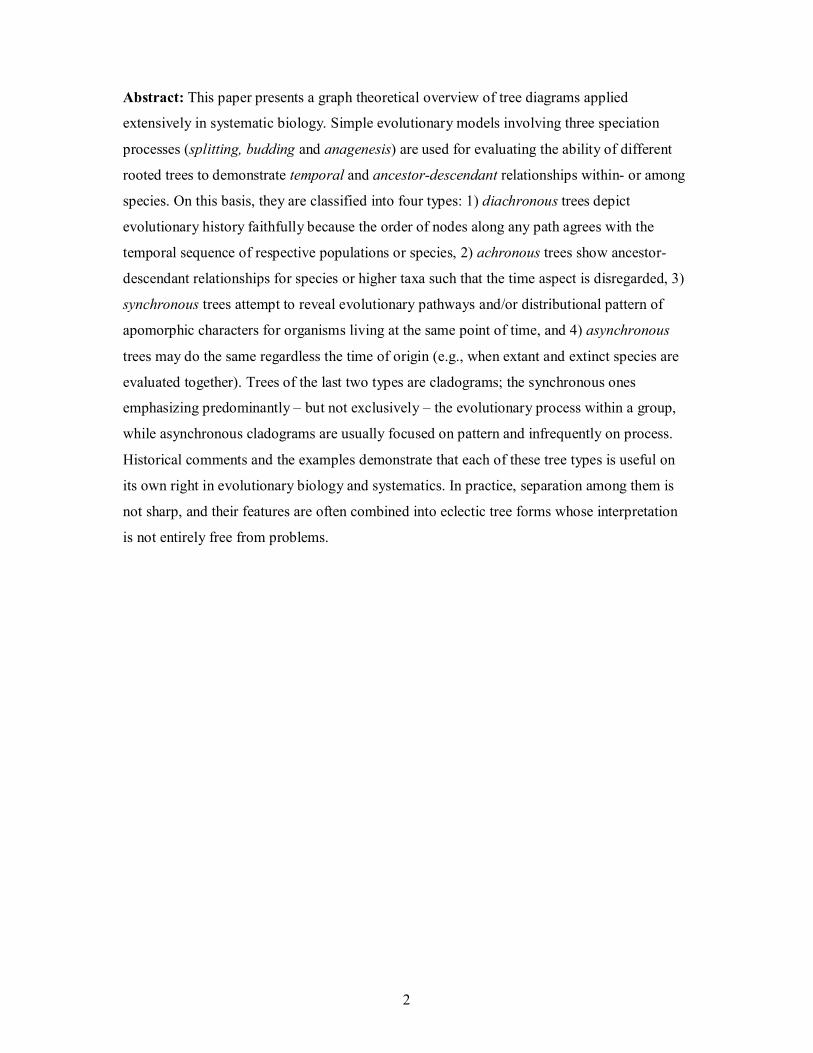
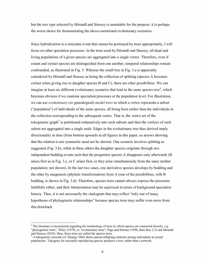
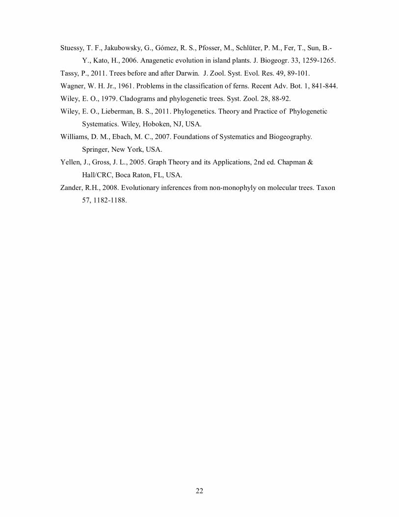
As a critique of the cladistic approach, Hörandl and Stuessy (2010) present several example
trees (their Fig. 4, partly reproduced here as Fig. 2, right column) to show that cladograms
cannot reflect evolutionary processes and patterns faithfully because the same cladogram (Fig.
2, left column) obtains for very different evolutionary relationships3. Speciation events
examined by those authors include budding (or branching off: the ancestor gives rise to a
daughter species and remains extant), splitting (or bifurcation: the ancestor ceases to exist
while splitting into two descendants), and merging (hybridization). It is claimed that a
cladogram may reflect evolutionary relationships correctly only for symmetric splitting events
(as originally expressed by Hennig’s (1966) deviation rule or cleavage model), whereas in
other cases “evolutionary trees may differ in their topology from the respective cladograms”.
The implicit conclusion is that cladograms are of limited use in evolutionary systematics.
However, I will show that it is not the cladogram that reflects evolutionary history incorrectly,
2 Nevertheless, the entire „Tree of Life” is often portrayed as an unrooted tree. Without directionality of edges, however, we cannot examine the temporal aspects and ancestor-descendant relations which are of primary concern in this paper. 3 I just note that the issue is not new, in fact several authors tried to evaluate cladogram performance by considering the same type of trees Hörandl and Stuessy were using (for example, Platnick 1977; Wiley 1979).
6
but the tree type selected by Hörandl and Stuessy is unsuitable for the purpose: it is perhaps
the worst choice for demonstrating the above-mentioned evolutionary scenarios.
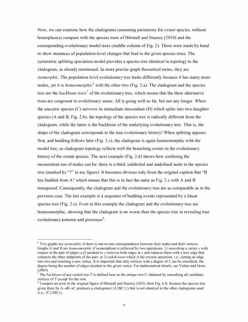
Since hybridization is a reticulate event that cannot be portrayed by trees appropriately, I will
focus on other speciation processes. In the trees used by Hörandl and Stuessy, all dead and
living populations of a given species are aggregated into a single vertex. Therefore, even if
extant and extinct species are distinguished from one another, temporal relationships remain
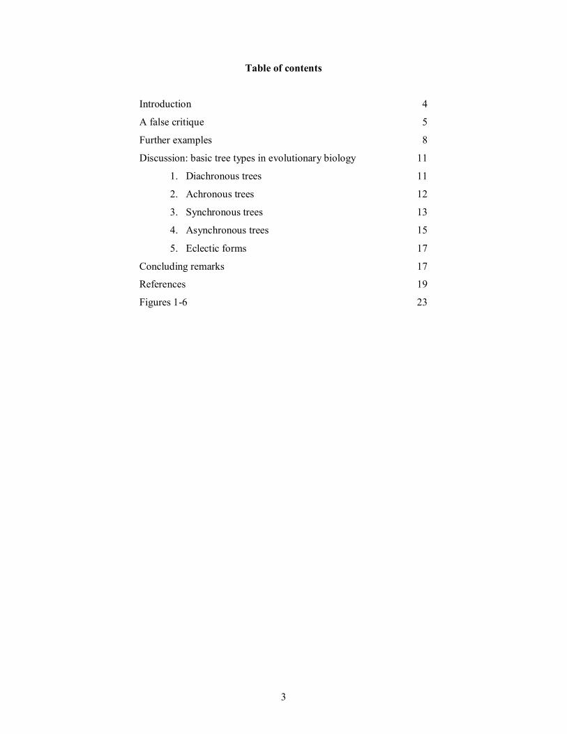
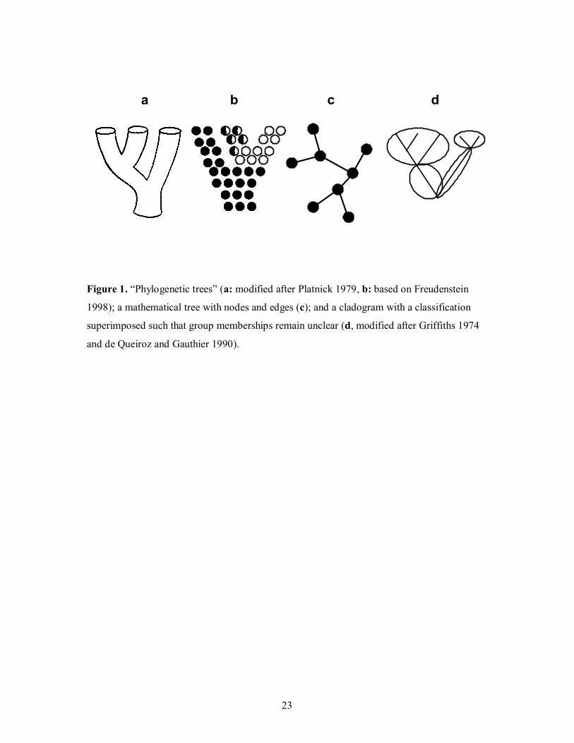
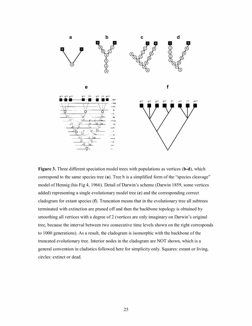
confounded, as illustrated in Fig. 3. Whereas the small tree in Fig. 3.a is apparently
considered by Hörandl and Stuessy as being the reflection of splitting (species A becomes
extinct when giving rise to daughter species B and C), there are other possibilities. We can
imagine at least six different evolutionary scenarios that lead to the same species tree4, which
becomes obvious if we examine speciation processes at the population level. For illustration,
we can use evolutionary (or genealogical) model trees in which a vertex represents a subset
(“population”) of individuals of the same species, all being born earlier than the individuals in
the collection corresponding to the subsequent vertex. That is, the vertex set of the
tokogenetic graph5 is partitioned exhaustively into such subsets and then the vertices of each
subset are aggregated into a single node. Edges in the evolutionary tree thus derived imply
directionality in time (from bottom upwards in all figures in this paper, so arrows showing
that the relation is not symmetric need not be shown). One scenario involves splitting as
suggested (Fig. 3.b), while in three others the daughter species originate through two
independent budding events such that the progenitor species A disappears only afterwards (B
arises first as in Fig. 3.c, or C arises first, or they arise simultaneously from the same mother
population; not shown). In the last two cases, one derivative species develops by budding and
the other by anagenesis (phyletic transformation) from A (one of the possibilities, with B
budding, is shown in Fig. 3.d). Therefore, species trees cannot always express the processes
faithfully either, and their interpretation may be equivocal in terms of background speciation
history. Thus, it is not necessarily the cladogram that may reflect “only one of many
hypotheses of phylogenetic relationships” because species trees may suffer even more from
this drawback.
4 The literature is inconsistent regarding the terminology of trees in which species are connected directly, e.g. “phylogenetic trees”, Wiley (1979), or “evolutionary trees”, Page and Holmes (1998, their Box 2.3) and Hörandl and Stuessy (2010). Here, these trees are called the species trees. 5 A tokogenetic network (cf. Hennig 1966) shows parent-offspring relations among individuals in sexual populations. Tokogeny for asexually reproducing species produces a tree, rather than a network.
7
Now, we can examine how the cladograms (assuming parsimony for extant species, without
homoplasies) compare with the species trees of Hörandl and Stuessy (2010) and the
corresponding evolutionary model trees (middle column of Fig. 2). These were made by hand
to show instances of population-level changes that lead to the given species trees. The
symmetric splitting speciation model provides a species tree identical in topology to the
cladogram, as already mentioned. In more precise graph theoretical terms, they are
isomorphic. The population level evolutionary tree looks differently because it has many more
nodes, yet it is homeomorphic6 with the other two (Fig. 2.a). The cladogram and the species
tree are the backbone trees7 of the evolutionary tree, which means that the three alternative
trees are congruent in evolutionary sense. All is going well so far, but not any longer. When
the ancestor species (C) survives its immediate descendant (D) which splits into two daughter
species (A and B, Fig. 2.b), the topology of the species tree is radically different from the
cladogram, while the latter is the backbone of the underlying evolutionary tree. That is, the
shape of the cladogram corresponds to the true evolutionary history! When splitting appears
first, and budding follows later (Fig. 2.c), the cladogram is again homeomorphic with the
model tree, so cladogram topology reflects well the branching events in the evolutionary
history of the extant species. The next example (Fig. 2.d) shows how confusing the
inconsistent use of nodes can be: there is a third, unlabeled and undefined node in the species
tree (marked by “?” in my figure). It becomes obvious only from the original caption that “B
has budded from A” which means that this is in fact the same as Fig. 2.c with A and B
transposed. Consequently, the cladogram and the evolutionary tree are as comparable as in the
previous case. The last example is a sequence of budding events represented by a linear
species tree (Fig. 2.e). Even in this example the cladogram and the evolutionary tree are
homeomorphic, showing that the cladogram is no worse than the species tree in revealing true
evolutionary patterns and processes8.
6 Two graphs are isomorphic if there is one-to-one correspondence between their nodes and their vertices. Graphs G and H are homeomorphic if isomorphism is achieved by two operations: 1) smoothing a vertex v with respect to the pair of edges (e,f) incident to v removes both edges at v and replaces them with a new edge that connects the other endpoints of the pair; or 2) subdivision which is the reverse operation, i.e., cutting an edge into two and inserting a new vertex. It is important that only vertices with a degree of 2 can be smoothed, the degree being the number of edges incident to the given vertex. For mathematical details, see Yellen and Gross (2005). 7 The backbone of any rooted tree T is defined here as the unique tree U obtained by smoothing all candidate vertices of T except for the root. 8 I suspect an error in the original figure of Hörandl and Stuessy (2010, their Fig. 4.f), because the species tree given there by ABC produces a cladogram ({A{BC}}) that is not identical to the other cladograms used (i.e., {C{AB}}).
8
While the topology of cladograms and the population-level evolutionary trees is comparable
in all cases discussed above, there are remarkable differences in character distributions on the
cladograms. In other words, in examining the cladogram not only the topology deserves
attention. If changes from the plesiomorphic state to the apomorphic are shown by small tick
marks on edges in the usual manner (the number of marks on each edge is its weight or
length), we see that all cladograms represent different synapomorphy schemes. The
distribution of tick marks on the tree gives some insight into potential background processes –
at least for the extant species. In particular, it is recognized easily that budding manifests itself
as a lacking autapomorphy on the edge incident to the mother species (zero-length edge),
which has long been known in cladistics (as visualized, for example, by the groundplan-
divergence analysis of Wagner 1961).
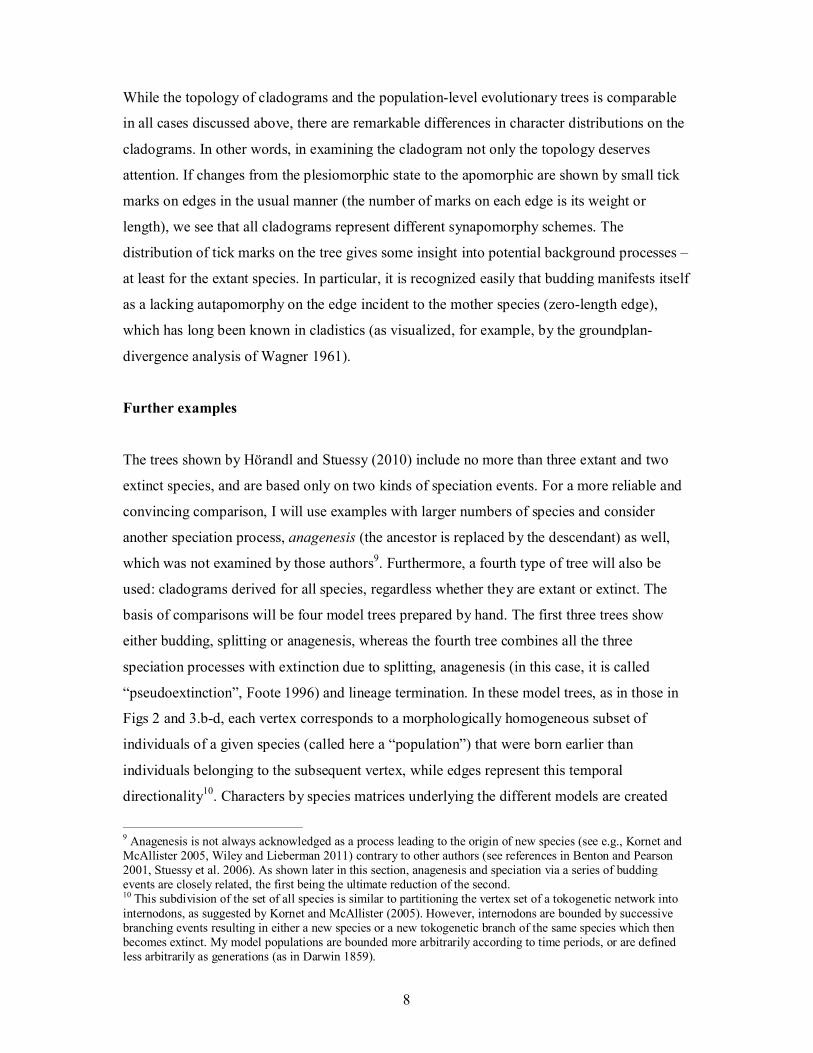
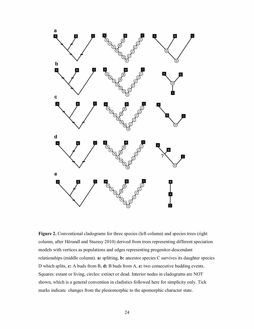
Further examples
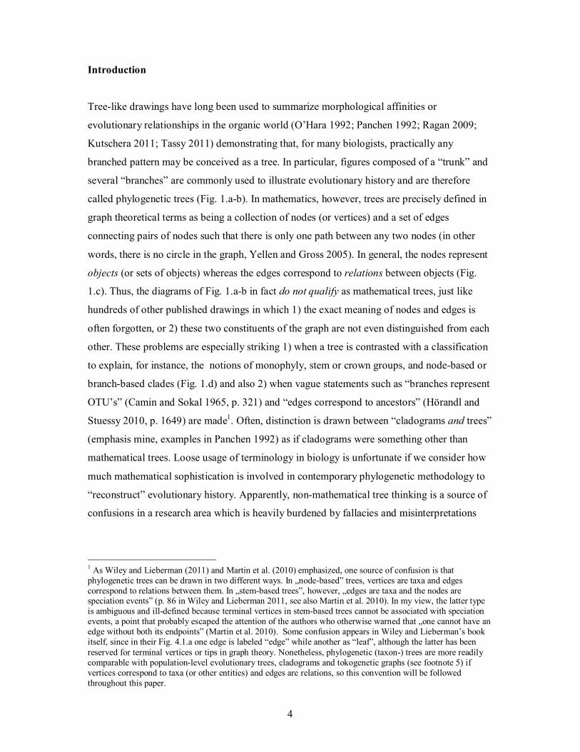
The trees shown by Hörandl and Stuessy (2010) include no more than three extant and two
extinct species, and are based only on two kinds of speciation events. For a more reliable and
convincing comparison, I will use examples with larger numbers of species and consider
another speciation process, anagenesis (the ancestor is replaced by the descendant) as well,
which was not examined by those authors9. Furthermore, a fourth type of tree will also be
used: cladograms derived for all species, regardless whether they are extant or extinct. The
basis of comparisons will be four model trees prepared by hand. The first three trees show
either budding, splitting or anagenesis, whereas the fourth tree combines all the three
speciation processes with extinction due to splitting, anagenesis (in this case, it is called
“pseudoextinction”, Foote 1996) and lineage termination. In these model trees, as in those in
Figs 2 and 3.b-d, each vertex corresponds to a morphologically homogeneous subset of
individuals of a given species (called here a “population”) that were born earlier than
individuals belonging to the subsequent vertex, while edges represent this temporal
directionality10. Characters by species matrices underlying the different models are created
9 Anagenesis is not always acknowledged as a process leading to the origin of new species (see e.g., Kornet and McAllister 2005, Wiley and Lieberman 2011) contrary to other authors (see references in Benton and Pearson 2001, Stuessy et al. 2006). As shown later in this section, anagenesis and speciation via a series of budding events are closely related, the first being the ultimate reduction of the second. 10 This subdivision of the set of all species is similar to partitioning the vertex set of a tokogenetic network into internodons, as suggested by Kornet and McAllister (2005). However, internodons are bounded by successive branching events resulting in either a new species or a new tokogenetic branch of the same species which then becomes extinct. My model populations are bounded more arbitrarily according to time periods, or are defined less arbitrarily as generations (as in Darwin 1859).
9
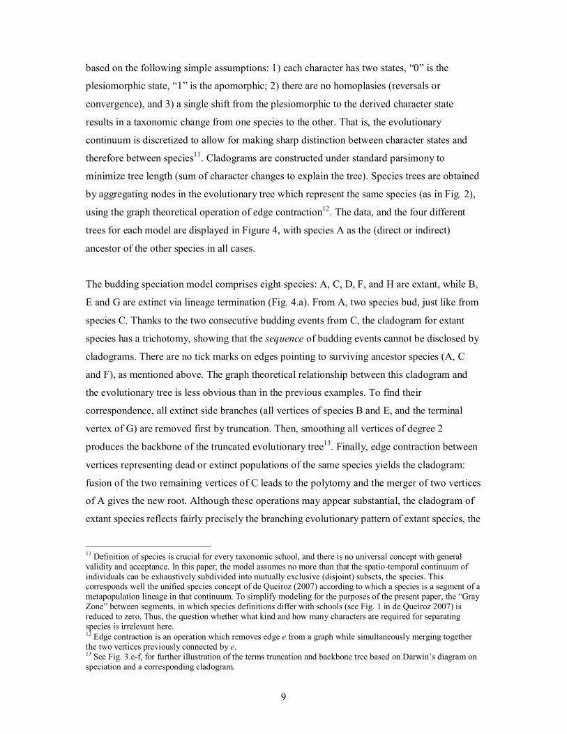
based on the following simple assumptions: 1) each character has two states, “0” is the
plesiomorphic state, “1” is the apomorphic; 2) there are no homoplasies (reversals or
convergence), and 3) a single shift from the plesiomorphic to the derived character state
results in a taxonomic change from one species to the other. That is, the evolutionary
continuum is discretized to allow for making sharp distinction between character states and
therefore between species11. Cladograms are constructed under standard parsimony to
minimize tree length (sum of character changes to explain the tree). Species trees are obtained
by aggregating nodes in the evolutionary tree which represent the same species (as in Fig. 2),
using the graph theoretical operation of edge contraction12. The data, and the four different
trees for each model are displayed in Figure 4, with species A as the (direct or indirect)
ancestor of the other species in all cases.
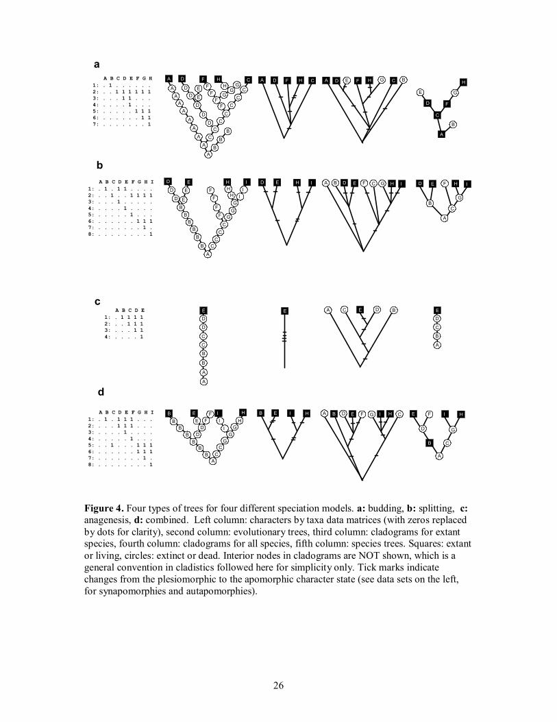
The budding speciation model comprises eight species: A, C, D, F, and H are extant, while B,
E and G are extinct via lineage termination (Fig. 4.a). From A, two species bud, just like from
species C. Thanks to the two consecutive budding events from C, the cladogram for extant
species has a trichotomy, showing that the sequence of budding events cannot be disclosed by
cladograms. There are no tick marks on edges pointing to surviving ancestor species (A, C
and F), as mentioned above. The graph theoretical relationship between this cladogram and
the evolutionary tree is less obvious than in the previous examples. To find their
correspondence, all extinct side branches (all vertices of species B and E, and the terminal
vertex of G) are removed first by truncation. Then, smoothing all vertices of degree 2
produces the backbone of the truncated evolutionary tree13. Finally, edge contraction between
vertices representing dead or extinct populations of the same species yields the cladogram:
fusion of the two remaining vertices of C leads to the polytomy and the merger of two vertices
of A gives the new root. Although these operations may appear substantial, the cladogram of
extant species reflects fairly precisely the branching evolutionary pattern of extant species, the
11 Definition of species is crucial for every taxonomic school, and there is no universal concept with general validity and acceptance. In this paper, the model assumes no more than that the spatio-temporal continuum of individuals can be exhaustively subdivided into mutually exclusive (disjoint) subsets, the species. This corresponds well the unified species concept of de Queiroz (2007) according to which a species is a segment of a metapopulation lineage in that continuum. To simplify modeling for the purposes of the present paper, the “Gray Zone” between segments, in which species definitions differ with schools (see Fig. 1 in de Queiroz 2007) is reduced to zero. Thus, the question whether what kind and how many characters are required for separating species is irrelevant here. 12 Edge contraction is an operation which removes edge e from a graph while simultaneously merging together the two vertices previously connected by e. 13 See Fig. 3.e-f, for further illustration of the terms truncation and backbone tree based on Darwin’s diagram on speciation and a corresponding cladogram.
10
exception being speciation involving two or more budding events from the same ancestor.
The cladogram of all species, extinct and extant, is homeomorphic with the evolutionary tree
with the exception of two trifurcations. The species tree is entirely atemporal because, for
example, ancestor species A survives three of its descendant species. This tree obtains directly
from the cladogram of all species by edge contraction: the fusion of nodes connected by edges
of zero length (those lacking tick marks for autapomorphic characters).
In the splitting model (Fig. 4.b), four species are ancestors (A, B, C, G) and species F
disappears due to lineage termination. The cladogram of extant species (D, E, H, I) correctly
recovers their backbone topology in the evolutionary tree. Contrary to the budding model, the
cladogram of all species is not homeomorphic with the evolutionary tree at all. Similarly to
the previous example, the species tree derives from the latter cladogram by edge contraction.
The species and evolutionary model trees are homeomorphic, as already observed in this
paper for other examples of splitting (Fig. 2.a, Fig. 3.a,b).
During anagenesis (Fig. 4.c), ancestor A runs through a transformation series ending with
species E. The corresponding cladogram is trivial since it has a single terminal species. Still, it
is homeomorphic with the evolutionary tree. The other cladogram, obtained for all species,
has zero-length edges incident to the extinct species and their contraction reproduces the
species tree. The latter, as for the splitting model, is homeomorphic with the evolutionary tree.
The combined model is constructed for six species such that each type of speciation events
appears twice (Fig. 4.d). In this case, the cladogram of recent species is a correct
representation of the backbone topology of the truncated evolutionary tree. The cladogram of
all species has three trifurcations, two pertaining to the splitting event and the other to
budding. As earlier, edge contractions reproduce the species tree, which differs topologically
from the evolutionary tree and the cladogram of extant species as well.
In the above examples, evolutionary model trees were drawn first, from which the data
matrices were compiled and the alternative trees were constructed. To obtain a more general
picture on the subject matter, we shall examine other possibilities to show that there is in fact
no one-to-one correspondence between data and evolutionary trees. Two cases in point
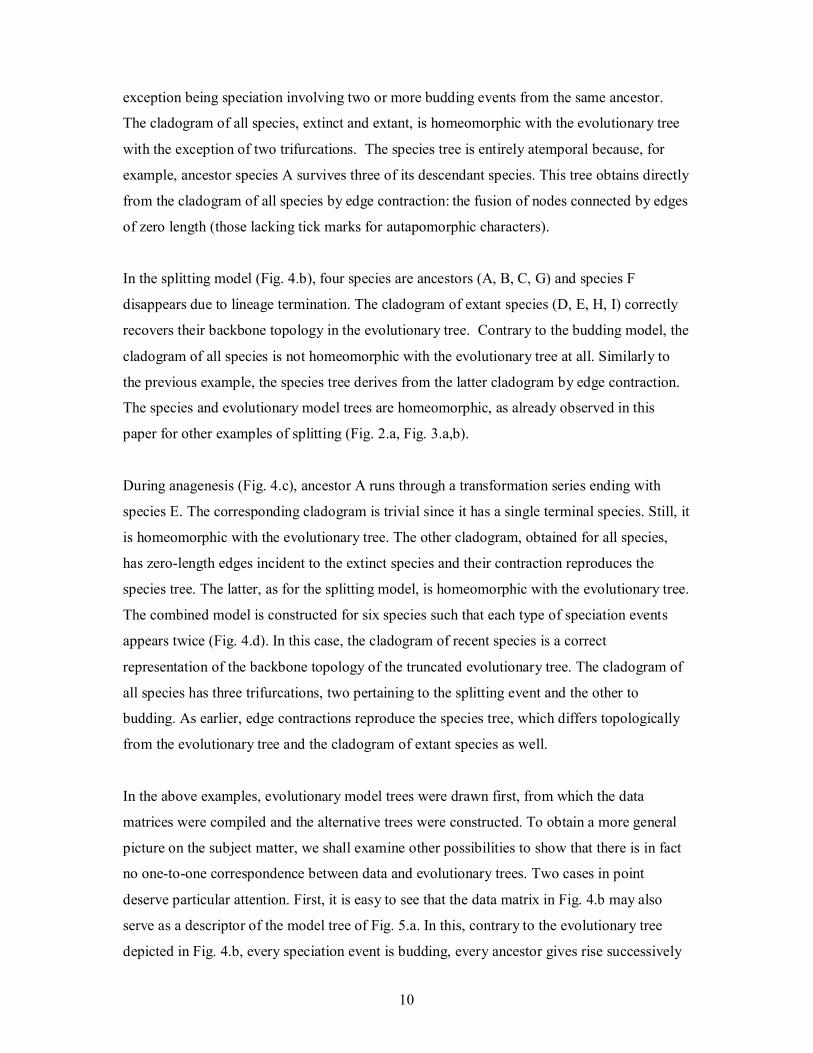
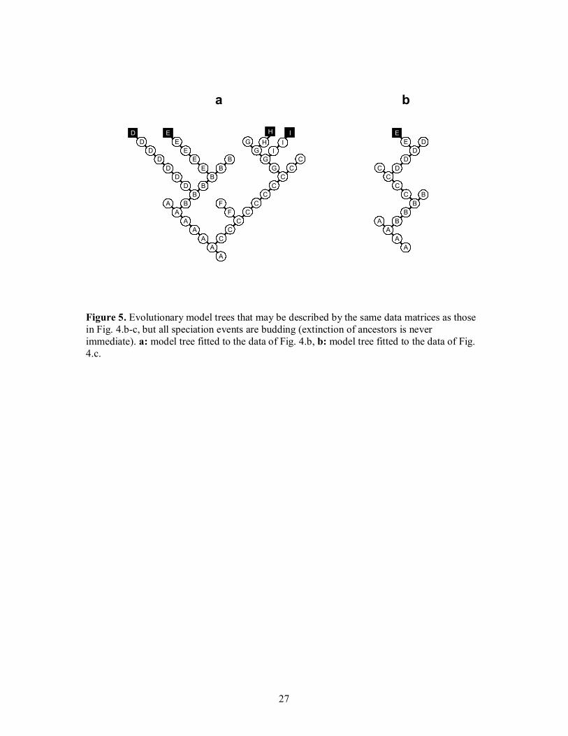
deserve particular attention. First, it is easy to see that the data matrix in Fig. 4.b may also
serve as a descriptor of the model tree of Fig. 5.a. In this, contrary to the evolutionary tree
depicted in Fig. 4.b, every speciation event is budding, every ancestor gives rise successively
11
to two descendants and then remains extant for a while. Note also that whereas the underlying
model has been altered, the two associated cladograms and the species tree remain unchanged.
We may conclude that species trees (as demonstrated already in Fig. 3) as well as both types
of cladograms cannot make distinction between splitting and a combined process involving
two consecutive budding events from the same ancestor and a delayed extinction of that
ancestor. This suggests clearly that splitting is an extreme case of this combined process, with
the topological distance between two consecutive budding events and the survival time of the
ancestor species reduced to zero. The backbone of the truncated evolutionary tree and the
regular cladogram are not homeomorphic, unless edge contraction reduces the number of
vertices for species A, B and G to 1. The same is true for the (non-truncated) evolutionary tree
and the cladogram of all species. The second example will illustrate another interesting
situation. The data in Fig. 4.c can also be conceived as describing a tree in which a series of
budding events is portrayed such that extinction of each ancestor is not immediate (Fig. 5.b).
In this tree, contrary to the evolutionary tree of Fig. 4.c, anagenesis is completely lacking.
Nevertheless, the two derived cladograms and the species tree remain the same as in Fig. 4.c.
This illustrates lucidly that these trees cannot distinguish between anagenesis and a series of
budding events with subsequent lineage termination of ancestors. A consequence is that
anagenesis can be conceived as a special case of a series of budding events such that survival
times of ancestor species are ultimately reduced to zero.
Discussion: basic tree types in evolutionary biology
Evaluation of the ability of different trees to show, summarize and even confuse background
speciation events allows conclusions to be made on 1) their general features and 2) their
performance under the specific models used. Considering the portrayed temporal relationships
among populations and species, extended to genera and higher taxa14, I suggest distinguishing
among four basic tree types, as follows.
1. Diachronous trees
Budding, splitting and anagenesis are population-level processes that can be best modeled by
Darwinian evolutionary trees in which nodes represent temporally separated populations and
edges correspond to progenitor-derivative relations (Fig. 2, middle column, Fig. 3.b-d, Fig. 4,
14 This paper is not concerned with rank-free classifications.
12
second column, Fig. 5) or Ancestor-Descendant Relations (ADR trees, Dayrat 2005). These
model trees are diachronous because they depict genealogical history over time correctly: the
temporal relationships between the units of study are preserved by the sequence of nodes
along any path from the root towards the leaves (i.e., terminal nodes or tips). The prototype of
these trees is the sole figure in “The Origin of Species” by Darwin (1859, see also Fig. 22 in
Ragan 2009 or Fig. 6 in Tassy 2011, partly reproduced in this paper, Fig. 3.e) – although it
does not satisfy fully the criteria for being a mathematical tree (in fact, it is not a single tree
but a forest, while most vertices are not shown). Actual evolutionary processes will never be
known to such fine details; nevertheless, these trees can be used efficiently in theoretical
discussions (Freudenstein 1998; Kornet and McAllister 2005; Podani 2010ab).
Mathematically, these graphs are spanning trees in which the nodes are biologically of similar
type (e.g., all of them represent populations, generations or internodons), and the number of
edges is one less than the number of nodes. It has been suggested (e.g., Dayrat 2005) that the
terms “evolutionary” or “phylogenetic” should be reserved to these trees, a convention
followed throughout this paper as well.
Diachrony cannot be shown by evolutionary trees at every taxonomic level. If we switch from
populations to species, then the graph can display proper temporal order only if the possibility
of speciation by budding is excluded. Thus, species trees may be correct diachronous
representations of evolutionary history only if ancestors disappear when giving rise to
descendants (anagenesis or splitting, Fig. 2.a, Fig. 4.b and c). Moreover, if we raise the
taxonomic level from species to genera or higher (i.e., aggregate several species into a single
node), then diachrony cannot be valid any longer for obvious reasons. Diachrony would
require that whenever a progenitor species A disappears after the speciation event, then all
other species in the same genus (or higher taxon) as A also go extinct in concert. Needless to
say, the probability of such coincidences rapidly diminishes when taxonomic rank increases
above the species level. Furthermore, paraphyly enters the scene, which brings us to the next
section.
2. Achronous trees
In case of budding (i.e., when the ancestor species survives the speciation event), species trees
may confuse temporal relationships: although the edges represent ancestor-descendant
relations, extinct and extant species may alternate along any path in the tree (Fig. 2.b and Fig.
4.a and d). Without having information on extinction, such trees may give the impression that
13
one species was followed by the other in time. Temporal relations are even more confounded
when species of the same genus or higher taxon are aggregated into a single node. It is
possible that the order of taxa along a path in such a tree conflicts with the order of geological
times in which some members of these taxa first appeared, hence the suggested name
achronous (Greek, “timeless”). A potential source of misinterpretation of these trees is that
they seem to suggest that the ancestor stopped evolving when giving rise to the
descendant(s)15. The prototype of achronous trees is the one drawn by Lamarck in 1809
(reproduced as Fig. 5 in Ragan 2009, or Fig. 4 in Tassy 2011), the first “phylogenetic” tree
ever published. Since that time, similar diagrams have dominated the biological literature,
before and after Darwin (for example, those drawn by Strickland and Haeckel). An interesting
historical aspect is that Wallace`s tree showing “affinities” within the bird group Fissirostres
was also of similar nature (Fig. 19 in Ragan 2009). Such trees are still popular today to
summarize major evolutionary advancements in function and form rather than descent (e.g.,
Cavalier-Smith 2010) and, hence, these are best termed as grade trees. Mathematically, these
graphs are spanning trees like evolutionary trees: all vertices are (ideally) of the same type
and edges may correctly link ancestor taxa with descendants at any taxonomic level. For
orders, the most famous example is perhaps the “cactus diagram” of angiosperms suggested
by Bessey (Fig. 3.2 in Judd et al. 2002) converted to a tree. Theoretically, a node
corresponding to a highly ranked taxon is an aggregate of nodes in evolutionary trees or
diachronous species trees, while in practice Besseyan diagrams may be derived from
cladograms (for example, Zander 2008). Taxa in grade trees may be monophyletic
(represented by nodes with a degree of 1) and paraphyletic (otherwise), while polyphyletic
groups correspond to single nodes mostly in achronous tree diagrams that are only of
historical importance (e.g., Haeckel’s many trees).
3. Synchronous trees
Based on the original proposal by Hennig (1966), cladograms are constructed to reveal the
evolutionary relationships for extant taxa, hence the name (synchrony refers to
“contemporaneous” organisms). These are represented by the leaves of the tree. Evolutionary
relationships between them are expressed by means of interior nodes, which can be
considered hypothetical ancestors, allowing the possibility that an ancestor is identical to an
15 As Judd et al. (2002, p. 44) noted, „such diagrams imply that groups that exist in the world today are the ancestors of other groups that also currently exist, which doesn’t make much sense in terms of evolutionary processes”.
14
extant taxon connected directly to it. A synchronous cladogram is thus a summary of a set of
Sister-Group Relationships (SGR-tree, Dayrat 2005), each expressed by two edges that
connect two terminal nodes (or sets of them, i.e., two clades) through an interior node. A
sister group hypothesis means that the groups involved are closer to each other than to any
other group. Mathematically, cladograms are Steiner trees in which the leaves and the interior
nodes are of different type. This difference is emphasized unintentionally in the cladistic
literature by not showing interior nodes explicitly. If the number of terminal nodes is n, then a
fully dichotomous Steiner tree has 2n-1 nodes and 2n-2 edges.
The examples in this paper demonstrated that a cladogram of contemporaneous organisms
may illustrate two phenomena simultaneously: 1) the sister group relationships and the tick
marks together reflect pattern (character distributions) as a result of evolution at a given point
of time, while 2) cladogram topology, as the backbone of the truncated evolutionary tree, plus
edge lengths (if available) depict the process (evolutionary pathways) by which that pattern
was generated. The ability to reflect background processes in this way is unequivocal for
splitting and anagenesis, but not always so for budding. If the still extant progenitor species
gives rise to two or more derivative species, then it manifests itself as a polytomy in the
cladogram and one edge with zero length. This happens whenever the data are uninformative
on branching sequences (Schmidt-Lebuhn 2012, see explanation to his Fig. 2). It has been
shown that the longer-lived is the ancestor, the more likely that several species will derive
from it by budding, and therefore the chance for obtaining polytomies is not negligible (Foote
1996). Consequently, trichotomy is not always a reflection of “unresolved” bifurcations
(considered by Hennig as a mere technical issue, but see Rieppel 2011), but a true three-
species relationship (see also Posada and Crandall’s [2001] similar arguments on gene trees).
In practice, perfect coincidence of pattern and process is more often the exception than the
rule: homoplasies in the cladogram can spoil interpretability of interior nodes as
synapomorphies. Also, many cladogram constructing methods do not even bother with
character distributions, because the process leading to the terminal objects is in focus
(Ereshefsky 2001; Rieppel 2010; Wiley and Lieberman 2011).
That synchronous cladograms reflect budding (except for polytomies), splitting and
anagenesis and their combinations in model situations correctly does not mean, of course, that
cladogram topology is fully informative on background speciation events. In fact, there are an
infinite number of possible evolutionary trees that produce the same cladogram (remember,
15
for example, that we do not know how many related species are extinct). However, it is easy
to see that the backbone trees of the truncated forms of all these alternatives are identical to
one another and isomorphic with the cladogram after applying edge contraction to their
vertices which represent dead or extinct populations of the same species, if such vertices exist.
This would not be possible at all if different speciation processes were represented incorrectly
by synchronous cladograms. Isomorphism is the key feature ensuring that synchronous
cladograms can be considered as attempts to “reconstruct phylogeny” (as authors of many
contemporary molecular cladistic papers put it)16 while all of us are aware that complete
reconstruction of the past is impossible.
When using a cladogram as a reference for classification, we should keep in mind that only
the leaves of the tree represent actual, classifiable objects, while interior nodes do not. In
other words, cladograms of contemporaneous organisms are useful to derive synchronous
classifications only. Therefore, if grouping is based on cladograms, I advise 1) to distinguish
such classifications from diachronous systems; 2) to distinguish monocladistic groups from
paracladistic ones: the first one is a complete sister group system, while the second is
incomplete and, consequently, 3) to separate monophyly from monoclady and paraphyly from
paraclady (see Podani 2009, 2010b, for more details).
Historically, prototypes of synchronous cladograms are those given in Hennig (1966). It is
nevertheless interesting to note that one of Haeckel’s trees (“Der Monophyletische
Stammbaum der Organismen”, Haeckel 1866, reproduced as Fig. 23 in Ragan 2009, Fig. 6 in
Kutschera 2011) may also be viewed as a cladogram: taxa are arranged at the tips of the tree,
all taxa are extant, none of them is derived from the other (contrary to Haeckel’s many other
grade trees, see Dayrat 2003), extinct side branches are almost completely missing, and there
is a superimposed high-level classification (3 major clades, and 19 smaller clades labeled).
4. Asynchronous trees
When extinct and extant organisms or, in general: taxa known from different geological ages,
are evaluated simultaneously by cladistic analysis, we are faced with radically different
possibilities for explanation and interpretation. Representing organisms of different times at
16 Dayrat (2005) pointed out that “most ‘phylogenetic trees’ or ‘phylogenies’ currently published simply are cladograms” which might confuse many scientists.
16
the same level violates synchrony, hence the suggested term asynchronous. The examples in
this paper demonstrated that under these circumstances
- a cladogram cannot always reveal the historical process although topologically it is
comparable with the evolutionary tree if all speciation events were budding,
- polytomies may result from both budding and splitting,
- zero length of terminal edges may reflect survival of ancestor species (budding), and
extinction of ancestor species (splitting or anagenesis) as well, and
- contraction of zero length edges establishes close relationship to grade trees, i.e.,
transfer from asynchronous to achronous topologies.
Examples demonstrated that an asynchronous tree topology and edge lengths may depict both
pattern and process simultaneously only if speciation is by budding. Otherwise, ancestors may
appear in false sister group relationship with descendants, and the cladogram cannot be
isomorphic with the backbone of the underlying evolutionary tree. Of course, this is a
conclusion from a model whereas in practice one can never be sure about past speciation
processes. Uncertainty exists, in general, even though in models ancestors are easy to
distinguish from descendants (zero-length edges are incident to ancestors in asynchronous
cladograms). This is not a problem for many systematists whose interest is focused on pattern
(character distributions, synapomorphies), entirely disregarding the evolutionary process
generating that pattern. The paradigmatic shift from process to pattern is behind the
development of transformed cladistics (see, e.g., Scott-Ram 1990), which has a not too distant
relationship to numerical taxonomy as well: classifiable objects are at the tips of the
cladogram, as in dendrograms obtained by hierarchical clustering. Often, asynchronous
cladograms are used as a basis for classification without reference to phylogeny, while groups
derived from them are still called „monophyletic” as opposed to “non-monophyletic”
(Williams and Ebach 2007)17. Nevertheless, asynchronous groups may be directly comparable
with those delineated on diachronous and achronous trees, which is not so with synchronous
ones. If asynchronous trees are not burdened with reversals and convergences, then
synapomorphies (i.e., characters with apomorphic state appearing for at least two species)
may be associated with interior nodes. As a prototype of asynchronous cladograms, I would
nominate the one for fossil horses suggested by Camin and Sokal (1965, their Fig. 4) in which
17 To resolve this ambiguity, I have suggested the use of terms monothety and polythety (Podani 2010a).
17
the tips of the tree represent taxa described from different geological times (from the
Oligocene to the Pliocene), both ancestors and descendants.
5. Eclectic forms
The four tree types do not always appear in pure form in the literature, because their
characteristics may show up simultaneously in the same graph in a wide variety of ways.
Especially common is the practice of combining cladogram properties with a grade tree18. In
such “hybrid” trees, unlabeled interior nodes (cladistic bifurcations or polytomies) appear
together with named interior nodes representing extinct or extant taxa, or both. Noted
examples are some “phylogenetic” classification trees of angiosperms (e.g., Takhtajan and
Cronquist, among others, see Figure 3.3 in Judd et al. 2002). Similar diagrams are quite often
used to display relationships of genera within a family (e.g., Pedaliaceae, Ihlenfeldt 2010).
Regarding the time aspect, these are eclectic because parts of the tree emphasize synchrony of
sister groups (or appear to do so) whereas other parts refer to the derivation of one group from
the other in a way that diachrony and achrony are not distinguished properly. For this reason,
interpretation of eclectic tree diagrams is not straightforward in most cases.
Concluding remarks
Whereas much has been said in the contemporary literature on the philosophical aspects of
evolutionary/ phylogenetic/ cladistic analysis, the graph theoretical side of the subject matter
has not yet received sufficient attention – even though tree graphs have long been used
paradigmatically as metaphors of order in the living (and extinct) world. This may have
serious consequences that are harmful to systematics and, in general, to biology. The problem
is rooted in that edges and nodes of the graphs are not always understood in accordance with
the common language of science, i.e., mathematics. In lack of a unified terminology that is
consistent with graph theory, mutual understanding among different schools of systematics is
impossible. For example, persisting terminological confusion over the meaning of trees, or
different parts of them, explains that participants in the controversy about paraphyly and
monophyly still “talk past each other” (Schmidt-Lebuhn 2012).
I used simple models of three speciation processes to generate tree diagrams which portray
within- and between species relationships differently. Examples demonstrated that
18 Note, however, that combining trees of the same type into a single one (e.g., consensus cladograms and supertrees) preserves the properties of the original trees.
18
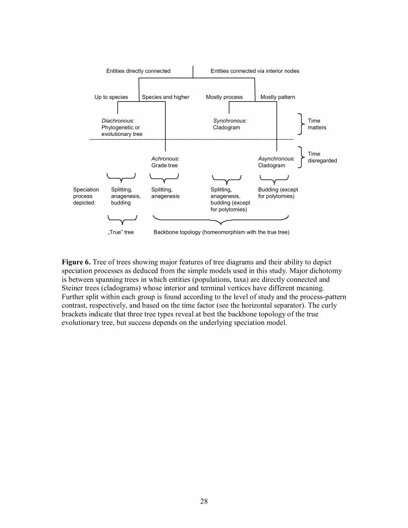
interpretation of these trees is constrained by their ability to reflect speciation processes and
ancestor-descendant relationships (Fig. 6). These phenomena can only be shown adequately
by diachronous trees in which nodes represent individuals, populations or, at most, species.
Such trees are, however, epistemiologically unknowable albeit useful in theoretical
discussions. Achronous trees expand the meaning of nodes to taxa higher than species, but the
cost is high: while ancestor-descendant relationships may be maintained (when species A in
taxon 1 is the ancestor of species B in taxon 2), temporal relationships between taxa 1-2 will
not be maintained in the tree, unless both of them are monotypic, and therefore paraphyly
becomes unavoidable. At the species level, the topology of diachronous and achronous trees is
comparable for anagenesis and splitting, but no so for budding. Thus, although both of them
are spanning trees (i.e., studied populations or taxa are connected directly), their interpretation
differs radically.
Synchronous trees (conventional Hennigian cladograms) can be used to generate hypotheses
on evolutionary processes. This may be achieved, for example, by finding synapomorphies for
entities ranging from individuals to high taxa living at a given point of time, but other,
probability-based strategies are also widely used especially at the molecular level. Cladogram
topology, if all sister-group relationships are depicted correctly, agrees with the backbone
topology of the truncated (true but unknown) evolutionary tree, with the exception of
polytomies caused by >1 budding events from the same ancestor species. Thus, the modeled
cases refute the common belief that cladograms can represent only divergence (splitting) and
that multifurcations always reflect phylogenetically “unresolved” situations. If a cladogram is
constructed for organisms of different times, then it may be primarily viewed as an
asynchronous summary of synapomorphies. Nevertheless, asynchronous cladograms may also
be identical in topology to the backbone phylogeny when no analyzed entity is ancestral to
any other via speciation by splitting or anagenesis. One should keep it mind that all
cladograms are Steiner trees: taxa are connected through interior vertices which should be
interpreted differently from terminal vertices.
Although recently the most important demarcation line within the domain of cladistic
approaches has been drawn between the so-called process cladistics and pattern cladistics (see
e.g., Ereshefsky 2001; Rieppel 2010), the present study demonstrated that distinction between
synchronous and asynchronous cladograms is perhaps more important in evolutionary
context. Synchrony always allows (although does not guarantee, of course) reconstruction of
19
evolutionary pathways which may then serve as a basis for classification, and a synchronous
summary may also reflect character distributions quite properly. That is, pattern and process
do not separate as sharply as previously suggested. An asynchronous analysis may very well
be a useful atemporal summary of the pattern of life, and process as well (for budding), but
there is always a risk to view the topology of asynchronous cladograms as being a
reconstruction of phylogeny. There is no ambiguity at all if we consider these cladograms as
classification trees, as originally proposed by pattern cladists.
My answer to the questions raised by Hörandl and Stuessy (2010) may be summarized as
follows. Conceptually, there is loss of information during transfer from the most detailed
evolutionary trees to grade trees and both types of cladograms. This means that none of the
latter three can recover underlying evolutionary processes fully – there are an infinite number
of possible evolutionary scenarios that lead to a given grade tree or a cladogram. The present
model situations demonstrate, however, that the risk of mistake is the smallest for
synchronous cladograms (unbiased towards any type of speciation processes examined here),
followed by asynchronous ones (biased towards budding), whereas grade trees (biased
towards splitting and anagenesis) can be drastically misleading even at the species level, not
to mention higher taxa. Nevertheless, each tree type has its own merits in revealing,
explaining or illustrating evolutionary and classificatory pattern of nature, and is therefore
useful under different circumstances. Mathematically they are closely related: graph
theoretical operations may be used to convert one tree type into the other. Therefore,
distinction among the four tree types is not necessarily sharp and, indeed, many published
diagrams combine their features. The ground is now open for a more detailed comparison of
tree types by using more realistic (e.g., stochastic) evolutionary models and tree
reconstruction procedures that rely not only on parsimony of character distributions.
Acknowledgements. I am grateful to three anonymous referees for their constructive
criticism of earlier versions of the manuscript. I also thank J. Garay for discussions. This
paper is dedicated to my mentor, Prof. L. Orlóci (University of Western Ontario) on the
occasion of his 80th birthday.
References
Benton, M. J., Pearson, P. N., 2001. Speciation in the fossil record. Trends Ecol. Evol. 16,
405-411.
20
Camin, J. H., Sokal, R. R., 1965. A method for deducing branching sequences in phylogeny.
Evolution 19, 311-326.
Cavalier-Smith, T., 2010. Deep phylogeny, ancestral groups and the four ages of life. Phil.
Trans. Roy. Soc. B. 365, 111–132.
Crisp, M. D., Cook, L. G., 2005. Do early branching lineages signify ancestral traits? Trends
Ecol. Evol. 20, 122-128.
Darwin, C., 1859. On the Origin of Species. John Murray, London, UK.
Dayrat, B., 2003. The roots of ‘Phylogeny’: how did Haeckel really build his trees? Syst. Biol.
52, 515-527.
Dayrat, B., 2005. Ancestor-descendant relationships in the reconstruction of the Tree of Life.
Paleobiol. 31, 347-353.
de Queiroz, K., 2007. Species concepts and species delimitation. Syst. Biol. 56, 879-886.
de Queiroz, K., Gauthier, J., 1990. Phylogeny as a central principle in taxonomy:
phylogenetic definitions of taxon names. Syst. Zool. 39, 307-322.
Ereshefsky, M., 2001. The poverty of the Linnaean hierarchy. Cambridge Univ. Press,
Cambridge, UK.
Foote, M., 1996. On the probability of ancestors in the fossil record. Paleobiol. 22, 141-151.
Freudenstein, J. V., 1998. Paraphyly, ancestors, and classification – a response to Sosef and
Brummitt. Taxon 47, 95-104.
Griffiths, G. C. D., 1974. On the foundations of biological systematics. Acta Biotheor. 23, 85-
131.
Haeckel, E., 1866., Generelle Morphologie der Organismen. G. Reimer, Berlin, Germany.
Hennig, W., 1966., Phylogenetic Systematics. Univ. Illinois Press, Urbana, IL, USA.
Hörandl, E., Stuessy, T. F., 2010. Paraphyletic groups as natural units of biological
classification. Taxon 59, 1641-1653.
Ihlenfeldt, H.-D., 2010. Pedaliaceae – evolution and phylogeny of the succulent genera.
Schumannia 6, 151-182.
Judd, W. S., Campbell, C.S. Kellogg, E.A., Stevens, P.F. Donoghue, M.J., 2002. Plant
Systematics. A Phylogenetic Approach. 2nd ed. Sinauer, Sunderland, MA, USA.
Kornet, D. J. and McAllister, J. W. 2005. The composite species concept: A rigorous basis for
cladistic practice. In: Teydon, T. A. C., Hemerik, L. (Eds.), Current Themes in
Theoretical Biology: A Dutch Perspective. Springer, Dordrecht, pp. 95-127.
Krell, F.-T., Cranston, P. S., 2004. Which side of the tree is more basal? Syst. Entomol. 29,
279-281.
21
Kutschera, U., 2011. From the scala naturae to the symbiogenetic and dynamic tree of life.
Biology Direct 6:33.
Lamarck, J.-B., 1809. Philosophie zoologique. Dentu, Paris.
Martin, J., Blackburn, D., Wiley, E. O., 2010. Are node-based and stem-based clades
equivalent? Insights from graph theory. Version 2. PLoS Curr. 2010 November 22
[revised 2011 March 18]; 2: RRN1196. doi: 10.1371/currents.RRN1196.
O’Hara, R. J., 1992. Telling the tree: Narrative representation and the study of evolutionary
history. Biol. Philos. 7, 135-160.
Omland, K. E., Cook, L. G., Crisp, M. D., 2008. Tree thinking for all biology: the problem
with reading phylogenies as ladders of progress. BioEssays 30, 854-867.
Page, R. D. M., Holmes, E. C. 1998. Molecular Evolution. A Phylogenetic Approach.
Blackwell, Oxford.
Panchen, A. L., 1992. Classification, Evolution, and the Nature of Biology. Cambridge
University Press, Cambridge, UK.
Platnick, N. I., 1977. Cladograms, phylogenetic trees, and hypothesis testing. Syst. Zool. 26,
438-442.
Platnick, N. I., 1979. Philosophy and the transformation of cladistics. Syst. Zool. 28, 537-546.
Podani, J., 2009. Taxonomy versus evolution. Taxon 54, 1049-1053.
Podani, J., 2010a. Monophyly versus paraphyly: discourse without end? Taxon 55, 1011-
1015.
Podani, J., 2010b. Taxonomy in evolutionary perspective. An essay on the relationships
between taxonomy and evolutionary theory. Synbiol. Hung. 6, 1-42.
Posada, D., Crandall, K. A., 2001. Intraspecific phylogenetics: Trees grafting into networks.
Trends Ecol. Evol. 16, 37-45.
Ragan, M. A., 2009. Trees and networks before and after Darwin. Biol. Direct. 4(1), 43.
Rieppel, O., 2010. The series, the network, and the tree: changing metaphors of order in
nature. Biol. Philos. 25, 475-496.
Rieppel, O., 2011. Willi Hennig’s dichotomization of nature. Cladistics 27, 103-112.
Sandvik, H., 2008. Tree thinking cannot be taken for granted: challenges for teaching
phylogenetics. Theory in Biosciences 127, 45-51.
Schmidt-Lebuhn, A. N., 2012. Fallacies and false premises—a critical assessment of the
arguments for the recognition of paraphyletic taxa in botany. Cladistics 28, 174-187.
Scott-Ram, N.R., 1990. Transformed Cladistics, Taxonomy, and Evolution. Cambridge Univ.
Press, Cambridge, UK.
22
Stuessy, T. F., Jakubowsky, G., Gómez, R. S., Pfosser, M., Schlüter, P. M., Fer, T., Sun, B.-
Y., Kato, H., 2006. Anagenetic evolution in island plants. J. Biogeogr. 33, 1259-1265.
Tassy, P., 2011. Trees before and after Darwin. J. Zool. Syst. Evol. Res. 49, 89-101.
Wagner, W. H. Jr., 1961. Problems in the classification of ferns. Recent Adv. Bot. 1, 841-844.
Wiley, E. O., 1979. Cladograms and phylogenetic trees. Syst. Zool. 28, 88-92.
Wiley, E. O., Lieberman, B. S., 2011. Phylogenetics. Theory and Practice of Phylogenetic
Systematics. Wiley, Hoboken, NJ, USA.
Williams, D. M., Ebach, M. C., 2007. Foundations of Systematics and Biogeography.
Springer, New York, USA.
Yellen, J., Gross, J. L., 2005. Graph Theory and its Applications, 2nd ed. Chapman &
Hall/CRC, Boca Raton, FL, USA.
Zander, R.H., 2008. Evolutionary inferences from non-monophyly on molecular trees. Taxon
57, 1182-1188.
23
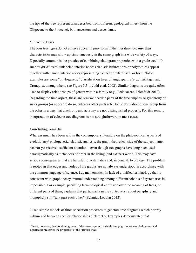
a b c d
Figure 1. “Phylogenetic trees” (a: modified after Platnick 1979, b: based on Freudenstein
1998); a mathematical tree with nodes and edges (c); and a cladogram with a classification
superimposed such that group memberships remain unclear (d, modified after Griffiths 1974
and de Queiroz and Gauthier 1990).
24
AD
DD
E
B C
C
C
CB
BCA
A
A
C
D
E
B CAB CA
B CA
AD
DD
C
B C
C
C
CB
BCA
A
A
C
D
C
A B
AB
BB
D
B C
C
C
CB
BCA
AA
CB CA
D
CB
A
AA
AA
D
B C
C
C
CB
BCA
AA
C
D
C
B
A
?
B CA
AA
AA
C
B C
C
C
CB
BCA
AA
C
C
A
BB CA
a
b
c
d
e
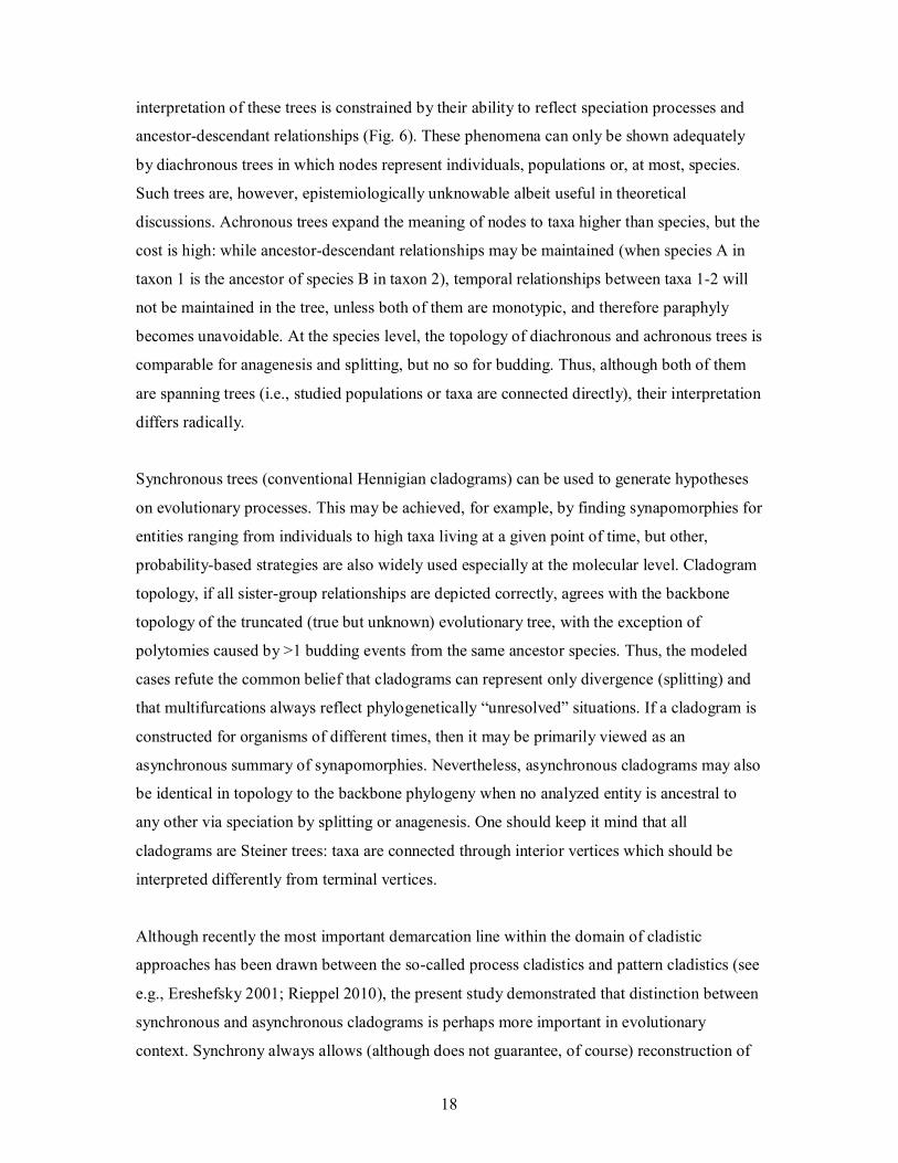
Figure 2. Conventional cladograms for three species (left column) and species trees (right
column, after Hörandl and Stuessy 2010) derived from trees representing different speciation
models with vertices as populations and edges representing progenitor-descendant
relationships (middle column). a: splitting, b: ancestor species C survives its daughter species
D which splits, c: A buds from B, d: B buds from A, e: two consecutive budding events.
Squares: extant or living, circles: extinct or dead. Interior nodes in cladograms are NOT
shown, which is a general convention in cladistics followed here for simplicity only. Tick
marks indicate changes from the plesiomorphic to the apomorphic character state.
25
A
A
A
AB
B
B
CC
C
AA
AA
AA
B
B
B
B
B
C
CC
C
AA
AA
B
B
B
B
B
C
C
C
C
A
B C
a b c d
e f
a14 q14 p14 b14 f14 o14 i14 m14
a14 q14 p14 b14 f14 o14 i14 m14
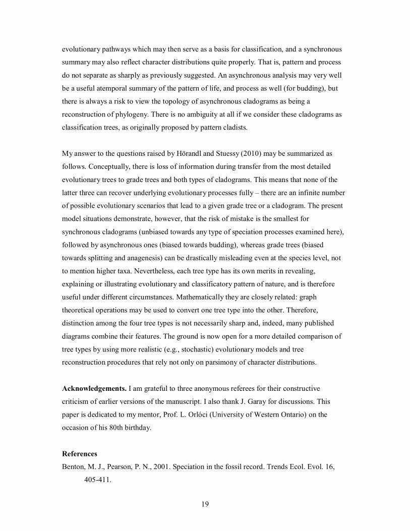
Figure 3. Three different speciation model trees with populations as vertices (b-d), which
correspond to the same species tree (a). Tree b is a simplified form of the “species cleavage”
model of Hennig (his Fig 4, 1966). Detail of Darwin’s scheme (Darwin 1859, some vertices
added) representing a single evolutionary model tree (e) and the corresponding correct
cladogram for extant species (f). Truncation means that in the evolutionary tree all subtrees
terminated with extinction are pruned off and then the backbone topology is obtained by
smoothing all vertices with a degree of 2 (vertices are only imaginary on Darwin’s original
tree, because the interval between two consecutive time levels shown on the right corresponds
to 1000 generations). As a result, the cladogram is isomorphic with the backbone of the
truncated evolutionary tree. Interior nodes in the cladogram are NOT shown, which is a
general convention in cladistics followed here for simplicity only. Squares: extant or living,
circles: extinct or dead.
26
B
A B C D E F G H1: . 1 . . . . . .2: . . 1 1 1 1 1 13: . . . 1 1 . . .4: . . . . 1 . . .5: . . . . . 1 1 16: . . . . . . 1 17: . . . . . . . 1
A B C D E F G H I1: . 1 . 1 1 . . . .2: . . 1 . . 1 1 1 13: . . . 1 . . . . .4: . . . . 1 . . . .5: . . . . . 1 . . .6: . . . . . . 1 1 17: . . . . . . . 1 .8: . . . . . . . . 1
A
A
A
A
C
D C
C
CC
B
D C
A
A
A
C
F H
AA
B
B
CA
D
D
G
FF
F GGH
E
E FD CA F H D CA F H BGE H
E
D
C
A
F
G
D E IH
A
B
E
ED
D
BB
C
G
E ID H
BB
BC
CC
GGF
F
FF
H IH I
A B ED F C G IH
A
B
ED F
C
G
IH
a
b
DD
A B C D E F G H I1: . 1 . 1 1 1 . . .2: . . . 1 1 1 . . .3: . . . . 1 . . . .4: . . . . . 1 . . .5: . . 1 . . . 1 1 16: . . . . . . 1 1 17: . . . . . . . 1 .8: . . . . . . . . 1
A B C D E1: . 1 1 1 12: . . 1 1 13: . . . 1 1 4: . . . . 1
A
B
C
D
A
B
C
D
E
A
B
C
D
EE A BC DE
BB
BB
A
B H
CC
GD
DG
BB
EH
c
d
I
GI
IF
FE
B HE I
B
HE I
A
F
D
C
G
HE IFD GBA C
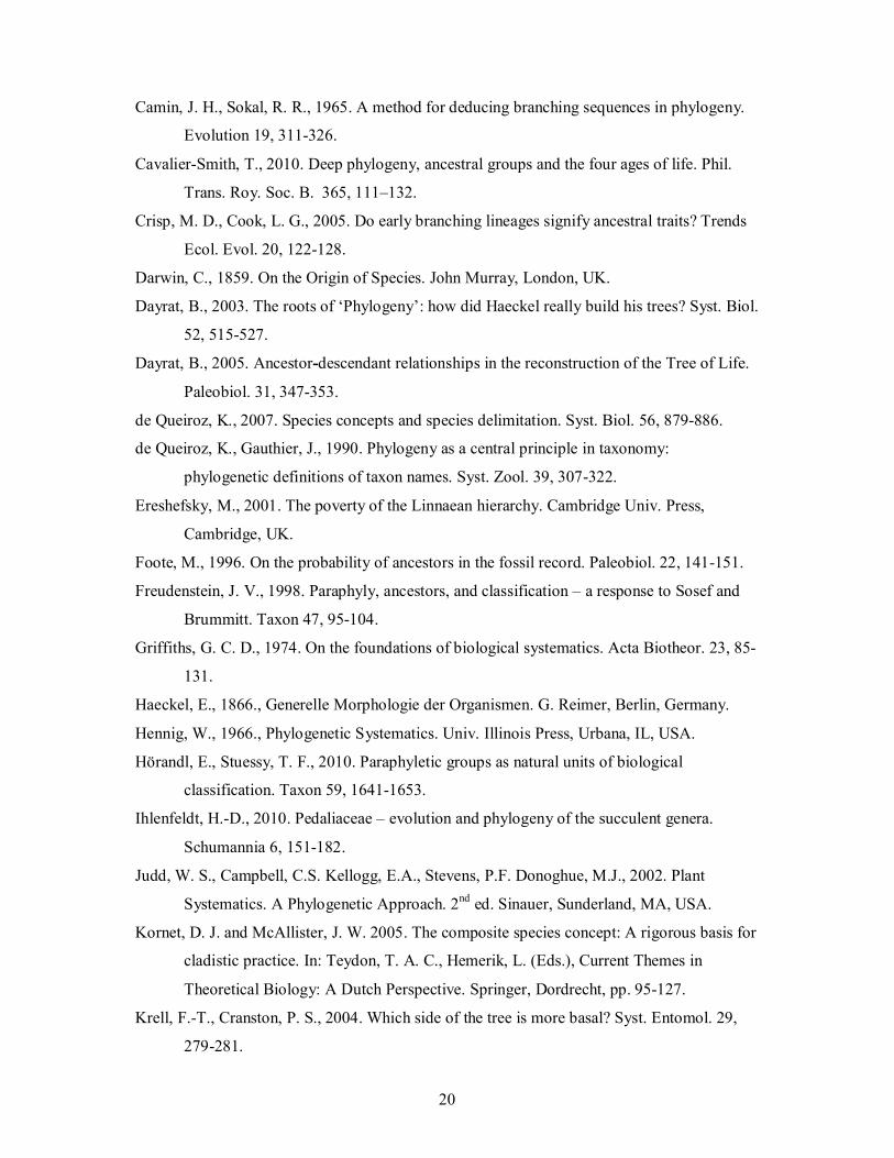
Figure 4. Four types of trees for four different speciation models. a: budding, b: splitting, c: anagenesis, d: combined. Left column: characters by taxa data matrices (with zeros replaced by dots for clarity), second column: evolutionary trees, third column: cladograms for extant species, fourth column: cladograms for all species, fifth column: species trees. Squares: extant or living, circles: extinct or dead. Interior nodes in cladograms are NOT shown, which is a general convention in cladistics followed here for simplicity only. Tick marks indicate changes from the plesiomorphic to the apomorphic character state (see data sets on the left, for synapomorphies and autapomorphies).
27
A B
C
D
E
F
G
HI
D E H I
AA
AA
AA
CC
CC
CC
C
BB
BB
DD
DD
D
BEE
E
F
CG
GG
C
I
AA
A
A BB
BBC
CC
C DD
DD
EE
a b
Figure 5. Evolutionary model trees that may be described by the same data matrices as those in Fig. 4.b-c, but all speciation events are budding (extinction of ancestors is never immediate). a: model tree fitted to the data of Fig. 4.b, b: model tree fitted to the data of Fig. 4.c.
28
Entities directly connected Entities connected via interior nodes
Up to species Species and higher Mostly process Mostly pattern
Diachronous: Phylogenetic orevolutionary tree
Achronous:Grade tree
Synchronous:Cladogram
Asynchronous:Cladogram
Timematters
Timedisregarded
Splitting,anagenesis,budding
Splitting,anagenesis
Splitting,anagenesis,budding (exceptfor polytomies)
Budding (exceptfor polytomies)
Speciationprocessdepicted:
„True” tree Backbone topology (homeomorphism with the true tree)
Figure 6. Tree of trees showing major features of tree diagrams and their ability to depict speciation processes as deduced from the simple models used in this study. Major dichotomy is between spanning trees in which entities (populations, taxa) are directly connected and Steiner trees (cladograms) whose interior and terminal vertices have different meaning. Further split within each group is found according to the level of study and the process-pattern contrast, respectively, and based on the time factor (see the horizontal separator). The curly brackets indicate that three tree types reveal at best the backbone topology of the true evolutionary tree, but success depends on the underlying speciation model.
Recommended