Trading in the Presence of Cointegration 12
by
Alexander Galenko 3
Operations Research and Industrial Engineering
The University of Texas at Austin, Austin, TX 78712
e-mail: [email protected]
Elmira Popova
Operations Research and Industrial Engineering
The University of Texas at Austin, Austin, TX 78712
phone: 512-471-3078, fax: 512-232-1489, e-mail: [email protected]
Ivilina Popova
Albers School of Business and Economics
Seattle University, Seattle, WA 98122
phone: 206-296-5736, fax: 206-296-5795, e-mail: [email protected]
1
Trading in the Presence of Cointegration
Abstract
The following research presents new properties of cointegrated time series that serve as
a basis for a novel high frequency trading strategy. The expected profit of this strategy
is always positive. Its practical implementation is illustrated using the daily closing prices
of four world stock market indexes. In-sample (as well as out-of-sample) results show that
the long-term dependencies of financial time series can be profitably exploited in a variant
of “pairs trading” strategy. This paper includes an extended empirical study that shows
the strategy’s performance as a function of its parameters. The backtests presented show
the daily profit and loss results for the period between 2001 to 2006. During that time the
strategy significantly outperformed a simple buy-and-hold of the individual indexes.
2

A popular alternative investment class has become hedge funds. One of the reasons for their
success is the use of a vast variety of strategies that explore different anomalies observed in
the financial markets. Focus has shifted to a group of strategies that rely on “quantitative
analysis” (also known as “statistical arbitrage”.) Quantitative analysis strategy develop-
ers use sophisticated statistical and optimization techniques to discover and construct new
algorithms. These algorithms take advantage of the short term deviation from the “fair”
securities’ prices. Pairs trading is one such quantitative strategy - it is a process of identi-
fying securities that generally move together but are currently ”drifting away”. They rely
on the validity of the assumption that due to the existing long-term relationship among the
securities, they will eventually revert to moving together once again. Exploring such spreads
has the potential to be profitable. Many equity hedge funds are using and have used similar
approaches. One of the commonly used methods for finding such spreads is based on correla-
tion. Since correlation is a short term measure, frequent rebalancing of a portfolio to reflect
the constantly changing spreads has become necessary, and as a result, high transaction costs
are usually observed. Additionally, there is evidence that the correlation could be a very
unreliable measure during financial market crises, like the collapse of the Long Term Capital
Management in 1998.
A measure of the long-term dependencies in financial time series is cointegration. Since
the seminal work of Engle & Granger (1987, 1991), many researchers in finance and eco-
nomics have used cointegration to model the dependencies between securities prices. Several
statistical test procedures for cointegration have been developed (see Engle & Granger 1991).
Tsay (2005) presented numerous examples and a detailed justification of using cointegration
in modeling financial time series. Alexander et al. (2002) used cointegration to construct
an index tracking portfolio. Alexander et al. (2002) showed that the optimal index tracking
portfolio has stationary tracking errors, and that efficient long-short hedge strategies can
be achieved with relatively few stocks and less turnover. Alexander (2001) discussed in de-
tail all the relevant published work in finance that used different properties of cointegration
for portfolio optimization or the construction of trading strategies. In summary, published
3

research on the use of cointegration in portfolio construction (specifically on constructing
time-dynamic trading strategies) is limited mainly to those aforementioned.
To better understand the relationship between cointegration and asset allocation, we
need to first describe two methods for asset allocation. The process of selecting a target
asset allocation or index is called strategic asset allocation. The variation from the target is
called tactical asset allocation. One can think of the strategic asset allocation as a process of
selecting the appropriate benchmark for a portfolio. For example, pension plans regularly go
through such a benchmark selection process in order to establish their investment policies.
Also, tactical asset allocation is usually identified with active portfolio management. For
example, how one should maintain the allocation of sixty percent stocks and forty percent
bonds over time comes into question.
Available research investigating the relationship between cointegration and asset alloca-
tion shows that cointegration affects strategic asset allocation. In other words, the decision
about optimal portfolio mix (or setting the appropriate benchmark) is influenced by the
common stochastic trend between assets. Lucas (1997) presented a model where a port-
folio manager maximized the expected utility of total earnings over a finite time period.
The associated time-series model captured cointegrating relations among the included assets.
He showed that cointegration affects strategic asset allocation while error-correction mainly
affects tactical asset allocation.
Using cointegration for trading or portfolio allocation implies the existence of a long-term
stochastic trend. In general, this is a contradiction with the hypothesis that the stock price
returns follow a random walk. Lo & MacKinley (1988) tested the random walk hypothesis
with weekly stock market returns by comparing variance estimators derived from data sam-
pled at different frequencies. If the stock returns followed a random walk, then the variance
should have grown with the square root of time. Lo & MacKinley (1988) rejected the ran-
dom walk hypothesis and showed that the rejection was due largely to the behavior of small
stocks. Additionally, they showed that the autocorrelations of individual securities were gen-
erally negative, and the autocorrelations of equally and positively weighted CRSP indexes
were positive.
Technical trading strategies that explore different short term market inefficiencies have
4

also been widely used by hedge fund managers. Gatev et al. (2006) showed how to construct
a “pairs trading” strategy with profits that typically exceeded conservative transaction-cost
estimates. Gatev et al. (2006) linked the profitability of this strategy to the presence of a
common factor in the returns different from conventional risk measures.
Lo & MacKinley (1990) showed a particular contrarian strategy that sold “winners” and
bought “losers” with a positive expected return, and that despite negative autocorrelations in
individual stock returns, weekly portfolio returns were strongly and positively autocorrelated
due to important cross-autocorrelations. Brown & Jennings (1989) showed that technical
analysis (or use of past prices to infer private information) had value in a model where prices
were not fully revealing, and where traders had rational conjectures about the relationship
of prices to signals. Conrad & Kaul (1998) analyzed a wide range of trading strategies from
1926-1989. They showed that momentum and contrarian strategies were equally likely to
be successful. Additionally, they found that the cross–sectional variation in mean-returns
of individual securities included in the strategies was an important determinant of their
profitability. Conrad & Kaul (1998) stated that the cross-sectional variation could potentially
account for the profitability of momentum strategies, and it could also be responsible for
some of the profits from price reversals to long-horizon contrarian strategies. Cooper (1999)
showed evidence of predictability by filtering lagged returns and lagged volume information
to uncover weekly overreaction profits on large cap stocks.
Our strategy evolves from the above described history of models and strategies. We be-
lieve that our theoretical and empirical results improve the understanding of how financial
markets adjust to new information. Our trading strategy exploits short-term pricing anoma-
lies revealed through deviation from the long-term stochastic trend. These anomalies are
consistent with the weak form of cross-market integration as documented in Chen & Knez
(1995). Our results also show support for the cointegrated type of asset pricing models as in
Bossaerts (1988).
Throughout this paper we derive new properties of cointegrated time series. These new
properties help to construct a dynamic trading strategy. It is proved that the expected re-
turn of the strategy is positive. Its practical implementation is reached using four world stock
market indexes, and presented is a detailed analysis of its performance. In-sample (as well
5
as out-of-sample) results show that long-term dependencies can be profitably exploited in a
variant of “pairs trading” strategy. The results do not vanish when we perform an out-of-
sample test. The problems with in-sample overfitting were well documented by Bossaerts &
Hillion (1999), Pesaran & Timmermann (1995), Cooper (1999), and Conrad et al. (2003).
Additionally, the “data snooping” problem and its relation to out-of-sample tests (as docu-
mented by Conrad et al. 2003, Cooper & Gulen 2006, Sullivan et al. 1999) is not a problem
for us, since our trading strategy is based on a theoretical relationship that we identify for
cointegrated time series. In particular, we prove that cointegration is a property related to
the 1st and 2nd moments of asset returns. In previous work the cointegration was viewed as
a property of the asset prices. We show that under certain assumptions the cointegration is
defined by the stochastic relationships among the asset returns.
This paper is organized as follows. First, the theoretical results are presented in §1. Then,
the strategy construction and the proof of its positive expected return are given in §2. Finally,
the detailed in-sample and out-of-sample empirical studies are in §3.
1 Stochastic Dependencies in Financial Time Series
Portfolio allocation models, like mean-variance (introduced by Markowitz (1952)) and Value-
At-Risk (first introduced by Jorion (2001)), included a measure of the risk associated with
the set of assets being considered. The standard measure included is the corresponding
covariance (or equivalently - the correlation) matrix. The covariance between two random
vectors X and Y is given by
Cov(X, Y ) = E{
(X − E[X]) (Y − E[Y ])T}
,
where E[X] stands for the expected value of the random vector X, and T denotes the matrix
transpose operator. It is well documented that the covariance (or correlation) is a measure
of the short-term linear dependencies (see Casella & Berger 2002, Theorem 4.5.7).
In contrast to correlation, cointegration is a measure of long-term dependencies (see Engle
& Granger 1991). We will briefly outline the notion of cointegration. In order to do so, we
need to first define stationary and integrated time series.
6

A stochastic process Yt is stationary if its first and second moments are time invariant: in
particular if E[Yt] = µ, ∀t and E[(Yt−µ)(Yt−h−µ)T ] = ΓY (h) = ΓY (−h)T , ∀t,h = 0, 1, 2, . . .,
where µ is a vector of finite mean terms, and ΓY (h) is a matrix of finite covariances. Such a
process is known as integrated of order 0 and denoted by I(0). Univariate process is called
integrated of order d, I(d), if in its original form it is non-stationary but becomes stationary
after differencing d times. If all elements of the vector Xt for t = 1, . . . , N , are I(1), and
there exists a vector b such that bT Xt is I(0), then the vector process Xt is said to be
cointegrated, and b is called the cointegrating vector. For example, two time series X and Y
are cointegrated if X, Y are I(1), and there exists a scalar b such that Z = X − bY is I(0).
Assume now that we have N ≥ 2 cointegrated financial assets, and their log-prices are
I(1) processes. It is widely assumed that stock returns are integrated of order 0, whereas the
stock prices are integrated of order 1 (see Alexander et al. 2002).
Denote the vector of the asset prices by Pt = {P 1t , . . . , PN
t }. Each of its elements
can be written as P it = P i
0ePt
j=0 rij , i = 1, . . . N , where r = {r1
t , . . . , rNt } are the contin-
uously compounded asset returns, and P 10 , . . . , PN
0 are the initial prices. (Without loss
of generality, we can assume that P 10 = . . . = PN
0 = 1). Then, the log-prices can be
written as lnP it = lnP i
0 +∑t
j=0 rij , i = 1, . . . , N . Denote the corresponding cointegrating
vector by b = (b1, . . . , bN ) . By the definition of cointegration, the resulting time series
Yt =∑N
i=1 bi lnP it will be stationary and integrated of order 0.
The next two propositions lead to derivations of new properties of cointegrated time series
that we later use for the construction of a new trading strategy.
Proposition 1 Assume that the log prices of N,N ≥ 2 assets, lnP i, i = 1, . . . , N , are coin-
tegrated with a cointegrating vector b. Let Yt =∑N
i=1 bi lnP it be the corresponding stationary
series, and {r1t , . . . , r
Nt }be the continuously compounded asset returns at time t > 0. Define
Zt = Yt − Yt−1 =∑N
i=1 birit. If limp→∞Cov[Yt, Yt−p] = 0, then
∞∑p=1
pCov[Zt, Zt−p] = −V arYt,
where Cov[Zt, Zt−p] =∑N
i=1
∑Nj=1 bibjCov[ri
t, rjt−p].
Proof: See the Appendix.
Proposition 1 is a technical result that we need to prove the next proposition. Intuitively,
it shows that the variance of the cointegration process (Yt) inadvertently defines the auto-
7

covariance of the asset returns.
Proposition 2 Assume lnP it , i = 1, . . . , N are the log-prices of N assets, and {r1
t , . . . , rNt }
are the continuously compounded asset returns at time t > 0. For some finite vector b, the
process Yt =∑N
i=1 bi lnP it , given lim
p→∞Cov[Yt, Yt−p] = 0, is stationary, and therefore the time
series of the assets’ log-prices are cointegrated, if and only if the process Zt =∑N
i=1 birit has
the following three properties:
(i) EZt = 0
(ii) V arZt = −2∑∞
p=1 Cov[Zt, Zt−p]
(iii)∑∞
p=1 pCov[Zt, Zt−p] < ∞.
Proof: See the Appendix.
As a result of proposition 2, it follows that cointegration is a property related to the 1st
and 2nd moments of asset returns. In previous work, cointegration was viewed as a property
of asset prices. Here we show that under certain assumptions, cointegration is defined by the
stochastic relationships among the returns.
Now presented is an example of cointegrated time series which illustrates the results of
the two propositions. Consider a model describing the log-return movements of two assets r1t
and r2t :
r1t = r2
t + c + (γ − 1)Yt−1 + ξ1t
r2t = µ2 + ξ2
t
Yt = c + γYt−1 + ξ1t ,
where µ2 is a real valued constant, and (ξ1t , ξ2
t ) are bivariate normal random variables with
mean vector 0, variances σ21, σ2
2, and covariance ρ. γ is a parameter of the AR(1) process Yt,
and it is a constant between 0 and 1, whereas c is a parameter of the AR(1) process Yt, a
constant.
The log-prices of these two assets are cointegrated of order one with cointegration vector
(1,−1). The corresponding theoretical moments are:
8
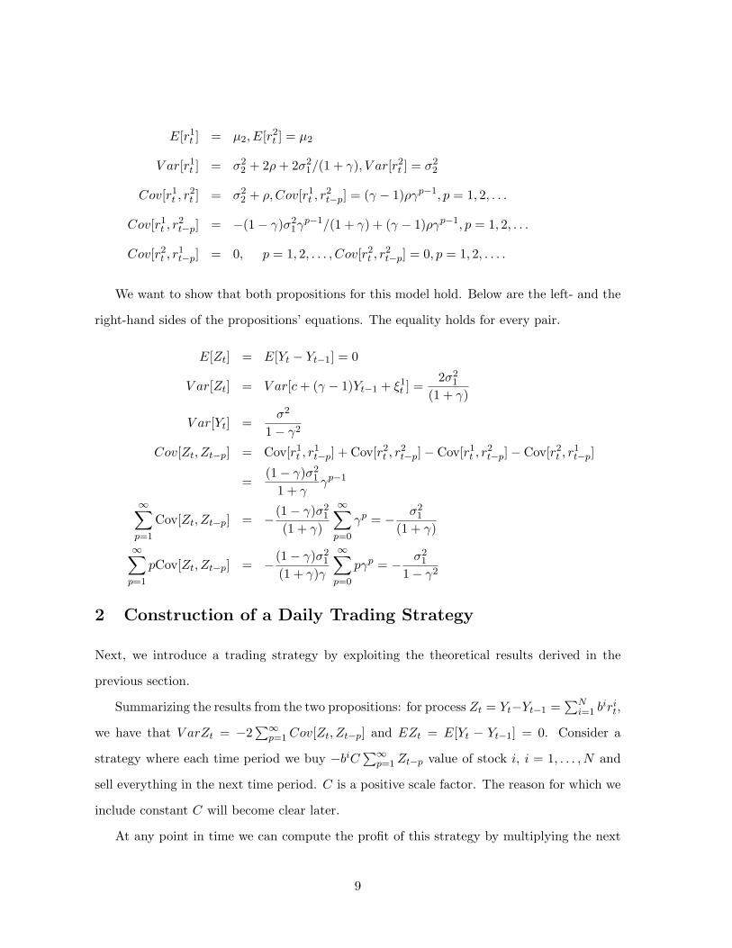
E[r1t ] = µ2, E[r2
t ] = µ2
V ar[r1t ] = σ2
2 + 2ρ + 2σ21/(1 + γ), V ar[r2
t ] = σ22
Cov[r1t , r
2t ] = σ2
2 + ρ,Cov[r1t , r
2t−p] = (γ − 1)ργp−1, p = 1, 2, . . .
Cov[r1t , r
2t−p] = −(1− γ)σ2
1γp−1/(1 + γ) + (γ − 1)ργp−1, p = 1, 2, . . .
Cov[r2t , r
1t−p] = 0, p = 1, 2, . . . , Cov[r2
t , r2t−p] = 0, p = 1, 2, . . . .
We want to show that both propositions for this model hold. Below are the left- and the
right-hand sides of the propositions’ equations. The equality holds for every pair.
E[Zt] = E[Yt − Yt−1] = 0
V ar[Zt] = V ar[c + (γ − 1)Yt−1 + ξ1t ] =
2σ21
(1 + γ)
V ar[Yt] =σ2
1− γ2
Cov[Zt, Zt−p] = Cov[r1t , r
1t−p] + Cov[r2
t , r2t−p]− Cov[r1
t , r2t−p]− Cov[r2
t , r1t−p]
=(1− γ)σ2
1
1 + γγp−1
∞∑p=1
Cov[Zt, Zt−p] = −(1− γ)σ21
(1 + γ)
∞∑p=0
γp = − σ21
(1 + γ)∞∑
p=1
pCov[Zt, Zt−p] = −(1− γ)σ21
(1 + γ)γ
∞∑p=0
pγp = − σ21
1− γ2
2 Construction of a Daily Trading Strategy
Next, we introduce a trading strategy by exploiting the theoretical results derived in the
previous section.
Summarizing the results from the two propositions: for process Zt = Yt−Yt−1 =∑N
i=1 birit,
we have that V arZt = −2∑∞
p=1 Cov[Zt, Zt−p] and EZt = E[Yt − Yt−1] = 0. Consider a
strategy where each time period we buy −biC∑∞
p=1 Zt−p value of stock i, i = 1, . . . , N and
sell everything in the next time period. C is a positive scale factor. The reason for which we
include constant C will become clear later.
At any point in time we can compute the profit of this strategy by multiplying the next
9

period return by the shares purchased:
πt =N∑
i=1
−biC
∞∑p=1
Zt−p
rit = −C
∞∑p=1
Zt−pZt.
Given that EZt = 0 and Cov[Zt, Zt−p] = EZtZt−p − EZtZt−p,p > 0, the expected profit of
this strategy is:
E [πt] = E
−C
∞∑p=1
Zt−pZt
= −C
∞∑p=1
Cov [Zt, Zt−p] =
= 0.5CV arZt.
Since V arZt and C are positive, the expected profit of the proposed strategy is always positive
and proportional to the scale factor C.
The reasoning behind this strategy is fairly simple. The cointegration relations between
time series imply that the time series are bound together. Over time the time series might
drift apart for a short period of time, but they ought to re-converge. The term∑∞
p=1 Zt−p
measures how far they diverge, and sign(−bi
∑∞p=1 Zt−p
)(where sign(a) = +1 if a > 0 and
−1 if a < 0) provides the direction of the trade for stock i. Specifically, +1 stands for a long
position, whereas −1 denotes a short trade. Such a trading strategy is a variant of pairs-
trading where one usually bets on identifying spreads that have gone apart but are expected
to mean revert in the future. The spreads of typical pairs-trading strategy get identified by
using correlation as a similarity measure and standard deviation as a spread measure. A
trade, for example, will be put in place if the assets are highly correlated but have gone apart
for more than 3 standard deviations. The trade will unwind when the assets converge or
some time limit is reached.
Our approach uses cointegration as a measure of similarity. Cointegration is the natural
answer of the question: How do we identify assets that move together? Proposition 2 provides
the answer of the question: How far do the assets have to diverge before a trade is placed?
As a result, the decision to execute a trade is driven by cointegration properties of the assets.
Having positive expected profit is excellent news for any strategy. The proposed strategy
has some shortcomings. The initial amount of money needed each period is a random variable,
and the resulting portfolio is not dollar neutral (i.e. the total dollar value of the long position
10

is not equal to the total dollar value of the short position.) To construct a dollar neutral
long-short portfolio, we will first partition the cointegrated time series into two sets L and S:
i ∈ L ↔ bi ≥ 0
i ∈ S ↔ bi < 0.
Next, depending on what set a given asset belongs to, we purchase the value of
−biCsign
∞∑p=1
Zt−p+1
/∑j∈L
bj , i ∈ L
biCsign
∞∑p=1
Zt−p+1
/∑j∈S
bj , i ∈ S.
The return of this modified strategy is identical to the proposed earlier. Hence, the expected
profit for that strategy is also positive.
Indeed (without loss of generality) assume that sign(∑∞
p=1 Zt−p
)= −1. The long returns
RLt and the short returns RS
t of our original strategy are
RLt =
∑i∈L−biC
∑∞p=1 Zt−pP
it+1/P i
t∑i∈L−biC
∑∞p=1 Zt−p
− 1 =∑
i∈L biP it+1/P i
t∑i∈L bi
− 1
RSt = 1−
∑i∈S −biC
∑∞p=1 Zt−pP
it+1/P i
t∑i∈S −biC
∑∞p=1 Zt−p
= 1−∑
i∈S biP it+1/P i
t∑i∈S bi
,
where sets S and L are defined above.
The modified strategy has the following returns from the short and long positions:
RLt =
∑i∈L
−biPj∈L bj Csign(
∑∞p=1 Zt−p)P i
t+1/P it∑
i∈L−biPj∈L bj Csign(
∑∞p=1 Zt−p)
− 1 =∑
i∈L biP it+1/P i
t∑i∈L bi
− 1
RSt = 1−
∑i∈S
biPj∈S bj Csign(
∑∞p=1 Zt−p)P i
t+1/P it∑
i∈SbiP
j∈S bj Csign(∑∞
p=1 Zt−p)= 1−
∑i∈S biP i
t+1/P it∑
i∈S bi.
The above derivations indicate the return of the modified strategy is the same as the original
one, therefore its expected profit is positive(since we proved that the expected return of the
original strategy is positive).
Now we can explain why we have included the constant C. In the modified strategy, every
time period the value of C is invested in short and long positions. Hence, the money needed
for each time period in order to execute the new strategy is a constant, and the portfolio we
obtain is dollar neutral.
11

In reality, we cannot compute the true value of∑∞
p=1 Zt−p (the cointegration vector b.)
We estimate them, and with the above theoretical results in mind, we propose the following
trading strategy:
• Step 1: using historical data, estimate the cointegration vector b.
• Step 2: using the estimated cointegration vector b̃ and historical data, construct Z̃t -
realizations of the process Zt =∑N
i=1 birit.
• Step 3: compute the final sum∑P
p=1 Z̃t−p+1, where P is a parameter.
• Step 4: partition the assets into two sets L and S (depending on values of b̃.)
• Step 5: buy (depending in which set the asset belongs to) the following number of
shares (round down to get integer number of shares):
−b̃iCsign
P∑p=1
Z̃t−p+1
/
P it
∑j∈L
b̃j
, i ∈ L
b̃iCsign
P∑p=1
Z̃t−p+1
/
P it
∑j∈S
b̃j
, i ∈ S.
• Step 6: close all the open positions the following trading day.
• Step 7: update the historical data set.
• Step 8: if it is time to re-estimate the cointegration vector (which happens every 22
trading days), go to step 1, otherwise go to step 2.
In the next section we describe the procedures used to test the strategy and present the
numerical results.
3 Trading Strategy - Performance and Analysis
To test the proposed trading strategy, we use historical data for four equity world indexes:
AEX4, DAX 5, CAC6 and FTSE7. Then, we present the results from several backtests. The
process of backtesting is an implementation of a trading strategy on available historical data
where we go back in time and start trading while pretending the past is now. It gives
12

us a picture of how the strategy would have performed if we were to use it in the past.
Such procedures are commonly used by financial professionals when a particular trading
rule/strategy is suggested for actual trading.
There are two types of tests: in-sample and out-of-sample. For in-sample backtesting, all
available data is used to estimate all the parameters of the strategy. Performance measures
are always better for in-sample testing, since we pretend that we can “see” the future by using
all the available historical information. Out-of-sample testing is a fair backtesting process
where information is available only up to the trading moment.
The number of days used to perform the estimation of the parameters is called a window
and is denoted by W . For example, a window size of 1000 (W = 1000) means that we used
the last 1000 daily observations for estimation.
Realizations from 01/02/1996 to 12/28/2006 were used for AEX, DAX, CAC and FTSE
indexes. Missing data due to difference in working days in different countries was filled using
one of the SPLUS FinMetrics functions that interpolates the missing value using a spline.
We also used the SPLUS vector auto regression estimation function to get the order of the
autoregressive process and its Johansen (1995) rank test to estimate the cointegration vector.
Trading for all tests starts on 11/06/2001 and ends on 12/28/2006. Transaction cost per share
was set to 1 cent. For out-of-sample testing we re-estimated the cointegration vector b every
22 days. The value of the long/short positions each day was set to 10,000,000 dollars (this
value may differ due to rounding.)
3.1 In-sample Results
To estimate the parameters for the in-sample test, we used all available historical data.
Results from this test for different values of P (the lag parameter) can be found in Tables 1
and 2, where Table 1 shows the results without transaction costs, and while Table 2 shows
the statistics after transaction costs of 1 cent per share. The long-term relationship between
the four indexes is estimated and described by the following cointegration vector:
Z = 3.69×AEX − 4.66× CAC + 13.57×DAX − 21.49× FTSE.
The resulting process Z is I(0).
13

Insert Tables 1 and 2 here.
Both tables report various performance measures: best and worst days, percentage of up
and down days, average daily gains and losses, volatility of positive and negative returns,
Sharpe and Sortino ratios, median, skewness and kurtosis of the daily returns, as well as the
average, standard deviation and maximum run down8.
As the value of the lag parameter changes from 10 to 40 days, the performance statistics
change as well. The best results (in terms of the corresponding Sharpe and Sortino ratios)
are for P = 30 days. For that particular value of the lag parameter, the Sharpe ratio is 1.15
and the Sortino ratio is 1.66. The annual return is 15.43% with a volatility of 13.44%. The
maximum number of days with consecutive negative returns is 8, and the average run down
days are 2. The performance statistics are based on 1320 trading days. The total return for
the covered period is 80.82% without transaction costs and 78.23% with transaction costs.
Table 2 shows in-sample results after transaction costs. Note that the results slightly
deteriorate, but the pattern stays the same. For that reason, we will report results without
transaction costs, since they are different for different types of investors9.
Figure 1 shows the profit and loss plot (P&L) for the strategy, as well as the four market
indexes. The trading strategy performs better than a simple buy-and-hold of the individual
indexes.
Insert Figure 1 here.
Table 3 shows the correlation between the strategy’s and individual indexes’ daily returns.
The results show that the performance of strategy is almost neutral or negatively correlated
with the individual indexes.
Insert Table 3 here.
3.2 Out-of-sample Results
An out-of-sample test is the only available tool to truly test how a strategy would have
performed if traded in the past. One of its drawbacks is the fact that we are testing the
performance of the strategy on one sample path only. Another drawback is that we face
14

the Uncertainty Principle of Heisenberg (see Bernstein 2007). The practical interpretation is
that one cannot measure the risk of an asset on the basis of past data alone. Once we enter
the first trade, effectively we are changing the market, and any type of backtest will not be
a perfect predictor about future performance.
We designed several out-of-sample backtests by changing the values of the critical pa-
rameters. All of them start on 11/06/2001. The amount of historical data used (or the size
of the window) varies from 1000 to 1500 days. For the first set of out-of-sample tests, we
used a sliding window to compute the parameters. Every 22 days the parameters of the
cointegration vector were re-estimated by using the last 1000, 1250 and 1500 days. A second
set of out-of-sample backtests used a cumulative window, where the initial window was 1000,
1250 and 1500 days. With every new trading day, the historical window used increased by
one day.
Tables 4, 5 and 6 show performance measures for the first set of out-of-sample tests with
sliding windows 1000, 1250 and 1500, respectively.
Insert Tables 4, 5 and 6 here.
Note that relative to the in-sample results, the strategy performance did not change
dramatically. For values of the lag parameter equal to 25 or 30 days, the Sharpe ratio varied
between 0.93 and 1.51, while the Sortino ratio varied between 1.26 and 2.26. The best results
in terms of Sharpe and Sortino ratio were obtained for a sliding window of 1000 days and a
lag parameter of 25 days. For this particular case the Sharpe ratio was 1.35 and the Sortino
ratio was 1.98.
Figure 2 presents the total return of the strategy (fixed window setup) as a function of
the two parameters of interest: the lag P and the window size W . Figure 3 is the same
for the cumulative window case. From here we can conclude that the lag parameter is more
important for the performance of the strategy than the window size.
Insert Figures 2 and 3 here.
Figure 4 shows the profit and loss for the strategy, when the lag parameter is 25 days and
the sliding window is 1000 days. Similar to the in-sample test, the strategy performs better
than buy-and-hold of the four indexes.
15

Insert Figure 4 here.
Table 7 shows the correlations of the strategy with the individual indexes. Similar to the
in-sample test, the strategy is almost neutral to the four market indexes.
Insert Table 7 here.
Figure 5 shows the time series of the cointegration vector.
Insert Figure 5 here.
Figures 4 and 5, if analyzed together, show an interesting property of the long-term
relationship between the indexes. The values of the cointegration vector do not change
substantially from 11/06/2001 to 3/25/2003. During this period, the strategy performs ex-
tremely well. During the same time period, all four indexes lose approximately 60% of their
value, while the strategy gains almost 50%. The cointegration vector changes dramatically on
3/25/2003 - a couple of days after the start of the Iraq war10. The next time point at which
a major adjustment in the parameters of the cointegration vector occurred is 8/16/2005,
almost one month after the terrorist attack in London.
Tables 8, 9 and 10 show performance measures for the second set of out-of-sample tests.
Cumulative windows are used starting with 1000, 1250 and 1500 days, respectively. The best
results in terms of Sharpe and Sortino ratio were obtained for lag parameter of 25 days and
cumulative window starting at 1500 days. The Sharpe ratio was 1.39, and the Sortino ratio
was 2.02.
Insert Tables 8, 9 and 10 here.
Figure 6 shows the profit and loss for the strategy when the lag parameter is 25 days,
and the cumulative window starts at 1500 days. Similar to the in-sample test, the strategy
performs better than buy-and-hold of the four indexes.
Insert Figure 6 here.
Table 11 shows the correlations of the strategy with the individual indexes. Similar to
the in-sample test, the strategy is almost neutral to the four market indexes.
16

Insert Table 11 here.
Figure 7 shows the time series of the cointegration vector.
Insert Figure 7 here.
With a cumulative window, the values of the cointegration vector are not highly variable.
The only period in time when some changes are visible is at the start of the Iraq war. One
can conclude from the two different designs of out-of-sample tests that the Iraq war caused
some major changes in the long-term relationship among financial assets.
Performance statistics from Tables 4 and 10 indicate that sliding window design is better
than cumulative window design. This outcome is not surprising if we refer to Proposition 1.
One of the assumptions there is that there will be a value of the lag parameter P for which
the long-term relationship will be almost non-existent. The results from the sliding window
design are empirical confirmation for that assumption.
4 Conclusion
We have derived a set of new properties of cointegrated financial time series. Using them
allowed us to create a new trading strategy. We proved that the expected profit of this
strategy is always positive, and we showed its practical implementation by using the daily
closing prices of four world stock market indexes.
In-sample and out-of-sample tests showed that the designed strategy significantly outper-
formed a simple buy-and-hold of the individual indexes. Additionally, the time series of the
cointegration vector exhibited how the strategy adapts to big stress events (like the start of
the Iraq war and the terrorist attack in London) in the financial markets.
17

5 Figure Legends
Figure 1: This figure shows the dynamics of the cumulative returns from the out-of-sample
backtest done with a lag of 25 days and a window size of 1000 days without transaction costs,
compared to the corresponding returns of the four indexes (AEX, CAC, DAX, FTSE.) The
horizontal axis is the time, and the vertical axis is the total cumulative return.
Figure 2: This figure is a 3 dimensional plot of the total return of the cointegration daily
strategy (out-of-sample test) as a function of the window size and the lag. The strategy was
run using the following values of the window size 1000, 1250 and 1500; the values of the lag
were 10,15,20,25,30,35 and 40.
Figure 3: This figure is a 3 dimensional plot of the total return of the cointegration daily
strategy (out-of-sample aggregate test) as a function of the window size and the lag. The
strategy was run using the following values of the window size 1000, 1250 and 1500; the values
of the lag were 10,15,20,25,30,35 and 40.
Figure 4: This figure shows the dynamics of the cumulative returns from the out-of-sample
backtest done with a lag of 25 days and a window size of 1000 days without transaction costs,
compared to the corresponding returns of the four indexes (AEX, CAC, DAX, FTSE). The
horizontal axis is the time, and the vertical axis is the total cumulative return..
Figure 5: This figure shows the estimated cointegration vector as a function of time. The
vector is re-estimated every 22 days using the Johansen cointegration rank test with data
from the previous 1000 days.
Figure 6: This figure shows the dynamics of the cumulative returns from the out-of-sample
backtest done with a lag of 25 days and a cumulative window starting at 1500 days without
transaction costs, compared to the corresponding returns of the four indexes (AEX, CAC,
DAX, FTSE.) The horizontal axis is the time, and the vertical axis is the total cumulative
return.
Figure 7: This figure shows the estimated cointegration vector as a function of time. The
vector is re-estimated every 22 days using the Johansen cointegration rank test using all data
up to the current time period.
18
6 Appendix
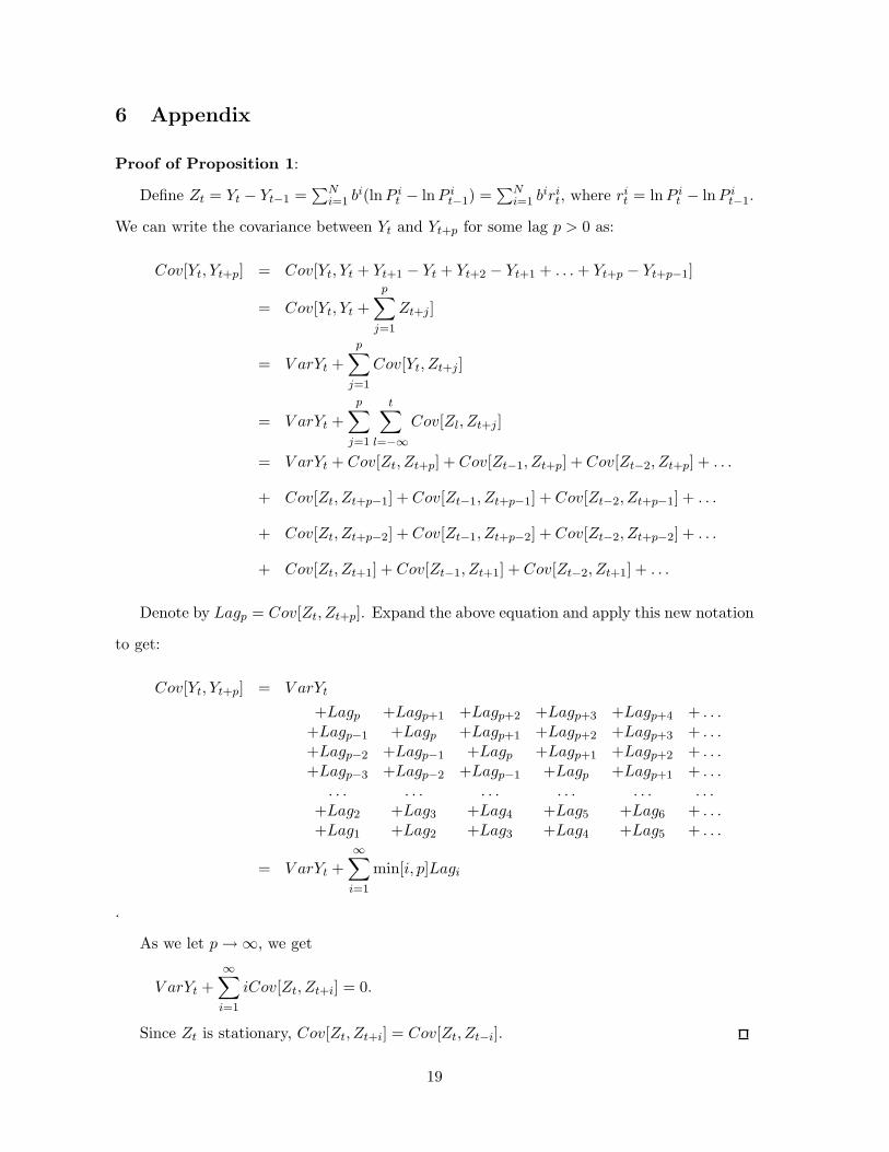
Proof of Proposition 1:
Define Zt = Yt − Yt−1 =∑N
i=1 bi(lnP it − lnP i
t−1) =∑N
i=1 birit, where ri
t = lnP it − lnP i
t−1.
We can write the covariance between Yt and Yt+p for some lag p > 0 as:
Cov[Yt, Yt+p] = Cov[Yt, Yt + Yt+1 − Yt + Yt+2 − Yt+1 + . . . + Yt+p − Yt+p−1]
= Cov[Yt, Yt +p∑
j=1
Zt+j ]
= V arYt +p∑
j=1
Cov[Yt, Zt+j ]
= V arYt +p∑
j=1
t∑l=−∞
Cov[Zl, Zt+j ]
= V arYt + Cov[Zt, Zt+p] + Cov[Zt−1, Zt+p] + Cov[Zt−2, Zt+p] + . . .
+ Cov[Zt, Zt+p−1] + Cov[Zt−1, Zt+p−1] + Cov[Zt−2, Zt+p−1] + . . .
+ Cov[Zt, Zt+p−2] + Cov[Zt−1, Zt+p−2] + Cov[Zt−2, Zt+p−2] + . . .
+ Cov[Zt, Zt+1] + Cov[Zt−1, Zt+1] + Cov[Zt−2, Zt+1] + . . .
Denote by Lagp = Cov[Zt, Zt+p]. Expand the above equation and apply this new notation
to get:
Cov[Yt, Yt+p] = V arYt
+Lagp +Lagp+1 +Lagp+2 +Lagp+3 +Lagp+4 + . . .+Lagp−1 +Lagp +Lagp+1 +Lagp+2 +Lagp+3 + . . .+Lagp−2 +Lagp−1 +Lagp +Lagp+1 +Lagp+2 + . . .+Lagp−3 +Lagp−2 +Lagp−1 +Lagp +Lagp+1 + . . .
. . . . . . . . . . . . . . . . . .+Lag2 +Lag3 +Lag4 +Lag5 +Lag6 + . . .+Lag1 +Lag2 +Lag3 +Lag4 +Lag5 + . . .
= V arYt +∞∑i=1
min[i, p]Lagi
.
As we let p →∞, we get
V arYt +∞∑i=1
iCov[Zt, Zt+i] = 0.
Since Zt is stationary, Cov[Zt, Zt+i] = Cov[Zt, Zt−i].
19

Proof of Proposition 2:
(⇐) Given
EZt = 0
−2∞∑
p=1
Cov[Zt, Zt−p] = V arZt and
∞∑p=1
pCov[Zt, Zt−p] = C < ∞,
it must be shown that Yt is stationary.
First, we show that E[Yt] is a constant over time. Indeed, for any p we have
E[Yt − Yt−p] = E[Yt − Yt−1 + Yt−1 − . . . + Yt−p+1 − Yt−p] = (1)p∑
i=1
E[Zt−i+1] = 0, (2)
which implies E[Yt] = E[Yt−p] for any p.
The variance of Yt is given by
V arYt = Cov[∑t
l=−∞ Zl,∑t
m=−∞ Zm] =+V arZt +Lag1 +Lag2 +Lag3 +Lag4 + . . .+Lag1 +V arZt +Lag1 +Lag2 +Lag3 + . . .+Lag2 +Lag1 +V arZt +Lag1 +Lag2 + . . .+Lag3 +Lag2 +Lag1 +V arZt +Lag1 + . . .
. . . . . . . . . . . . . . . . . .We will add to each line −
∑∞p=1 Cov[Zt, Zt−p] (we can do this since C is finite.) Now
use V arZt = −2∑∞
p=1 Cov[Zt, Zt−p] to get the result V arYt =∑∞
p=1 pCov[Zt, Zt−p].
Since∑∞
p=1 pCov[Zt, Zt−p] is constant, it follows that the variance of Yt is constant.
Now from the proof of proposition 1, we have that
Cov[Yt, Yt−p] = V arYt +∞∑i=1
min[i, p]Cov[Zt, Zt−i].
Obviously, Cov[Yt, Yt−p] depends on p only since V arYt is constant over time. Hence,
the process Yt is stationary.
20

(⇒) Given that Yt is stationary it must be shown that
−2∞∑
p=1
Cov[Zt, Zt−p] = V arZt and
∞∑p=1
pCov[Zt, Zt−p] = C < ∞.
By assumption, limp→∞Cov[Yt, Yt−p] = 0. Use Proposition 1 to get∑∞
p=1 pCov[Zt, Zt−p] =
V arYt, which is a constant.
What is left to show is that V arZt = −2∑∞
p=1 Cov[Zt, Zt−p]. Fix k, and consider
Cov
[t∑
l=t−k
Zl,
t∑m=−∞
Zm
].
Add∑k
p=1 Cov[Zt, Zt−p] to each term in∑t
l=t−k Zl to get
Cov
[t∑
l=t−k
Zl,
t∑m=−∞
Zm
]= −
k∑p=1
pCov[Zt, Zt−p]
+k+1∑m=1
[V arZt +
k∑l=1
Cov[Zt, Zt−l] +∞∑l=1
Cov[Zt, Zt−l]
].
As k →∞ we have that
limk→∞
Cov
[t∑
l=t−k
Zl,
t∑m=−∞
Zm
]= V arYt and
limk→∞
−k∑
p=1
pCov[Zt, Zt − p] = V arYt
hence,
limk→∞
(k + 1)
[V arZt +
k∑l=1
Cov[Zt, Zt−l] +∞∑l=1
Cov[Zt, Zt−l]
]= 0,
which implies that V arZt = −2∑∞
p=1 Cov[Zt, Zt−p].
21
References
Alexander, C. (2001), Market Models, John Wiley and Sons, LTD.
Alexander, C., Giblin, I. & Weddington, W. (2002), Cointegration and asset allocation: A
new active hedge fund strategy. ISMA Centre Discussion Papers in Finance Series.
Bernstein, P. L. (2007), ‘The price of risk and the Heisenberg uncertainty principle’, The
Journal of Portfolio Management 33, 1.
Bossaerts, P. (1988), ‘Common nonstationary components of asset prices’, Journal of Eco-
nomic Dynamics and Control 12, 347–364.
Bossaerts, P. & Hillion, P. (1999), ‘Implementing statistical criteria to select return forecasting
models: what do we learn?’, The Review of Financial Studies 12, 405–428.
Brown, D. & Jennings, R. (1989), ‘On technical analysis’, The Review of Financial Studies
2(4), 527–551.
Casella, G. & Berger, R. L. (2002), Statistical inference.
Chen, Z. & Knez, P. (1995), ‘Measurement of martket integration and arbitrage’, The Review
of Financial Studies 8, 287–325.
Conrad, J., Cooper, M. & Kaul, G. (2003), ‘Value versus glamour’, The Journal of Finance
pp. 1969–1995.
Conrad, J. & Kaul, G. (1998), ‘An anatomy of trading strategies’, The Review of Financial
Studies 11(3), 489–519.
Cooper, M. (1999), ‘Filter rools based on price and volume in individual security overreaction’,
The Review of Financial Studies 12, 901–935.
Cooper, M. & Gulen, H. (2006), ‘Is time-series-based predictability evident in real time?’,
Journal of Business 79, 1263–1292.
Engle, R. F. & Granger, C. W. J. (1987), ‘Portfolio selection’, Econometrica 55(2), 251–276.
22

Engle, R. F. & Granger, C. W. J. (1991), Long-run economic relationships, readings in
cointegration, Oxford University Press.
Gatev, E., Goetzmann, W. N. & Rouwenhorst, K. G. (2006), ‘Pairs trading: performance of
a relative-value arbitrage rule’, The Review of Financial Studies 19, 797–827.
Johansen, S. (1995), Likelihood-based inference in cointegrated vector autoregressive models,
Oxford University Press.
Jorion, P. (2001), Value at Risk: The New Benchmark for Managing Financial Risk, McGraw-
Hill Trade.
Lo, A. W. & MacKinley, A. C. (1988), ‘Stock market prices do not follow random walks:
evidence from a simple specification test’, Review of Financial Studies 1, 41–66.
Lo, A. W. & MacKinley, A. C. (1990), ‘When are contrarian profits due to stock market
overreaction?’, Review of Financial Studies 3, 175–205.
Lucas, A. (1997), Strategic and tactical asset allocation and the effect of long-run equi-
librium relations, Serie Research Memoranda 0042, Free University Amsterdam, Faculty
of Economics, Business Administration and Econometrics, De Boelelaan 1105, 1081 HV
Amsterdam.
Markowitz, H. M. (1952), ‘Portfolio selection’, Journal of Finance 7, 77–91.
Pesaran, M. & Timmermann, A. (1995), ‘Predictability of stock returns: robustness and
economic significance’, The Journal of Finance pp. 1201–1228.
Sullivan, R., Timmermann, A. & White, H. (1999), ‘Data-snooping, technical trading rule
performance, and the bootsrtap’, The Journal of Finance pp. 1647–1691.
Tsay, R. S. (2005), Analysis of financial time series, Wiley.
23

Notes
1This research has been partially supported by NSF grant number CMMI-0457558.
2The authors would like to thank Michael Cooper for helpful suggestions and comments.
3Corresponding author.
4The best-known index of Euronext Amsterdam, the AEX index, is made up of the 25most active securities in the Netherlands. This index provides a fair representation of theDutch economy.
5DAX 30 (Deutsche Aktien Xchange 30) is a Blue Chip stock market index consisting ofthe 30 major German companies trading on the Frankfurt Stock Exchange.
6The CAC 40, which takes its name from Paris Bourse’s early automation system CotationAssiste en Continu (Continuous Assisted Quotation), is a French stock market index. Theindex represents a capitalization-weighted measure of the 40 most significant values amongthe 100 highest market caps on the Paris Bourse.
7The FTSE 100 Index is a share index of the 100 most highly capitalized companies listedon the London Stock Exchange.
8Run down is the number of consecutive days with negative returns.
9Results with transaction costs are available from the authors upon request.
10Iraq war started on 3/19/2003.
24

Tables
Table 1: In-sample test results without transaction costs.
Performance Measures Lag Parameter P10 20 25 30 40
Best Day 6.09% 6.09% 6.09% 6.09% 6.09%Worst Day -4.64% -4.06% -4.06% -4.06% -4.06%Percentage of Up Days 51.14% 52.50% 52.35% 53.41% 53.03%Percentage of Down Days 48.86% 47.50% 47.65% 46.59% 46.97%Average Daily Gain 0.57% 0.59% 0.60% 0.60% 0.59%Standard Dev. of Positive Returns 9.97% 10.32% 10.58% 10.39% 10.20%Average Daily Loss -0.58% -0.56% -0.55% -0.55% -0.56%Standard Dev. of Negative Returns 9.81% 9.40% 9.06% 9.28% 9.53%Annual Return 2.83% 10.10% 12.90% 15.43% 11.70%Standard Dev. 13.47% 13.46% 13.45% 13.44% 13.45%Sharpe Ratio 0.21 0.75 0.96 1.15 0.87Sortino Ratio 0.29 1.07 1.42 1.66 1.23Skewness 0.12 0.36 0.48 0.39 0.32Kurtosis 5.30 5.26 5.23 5.25 5.27Average Run Down (days) 2 2 2 2 2Standard Dev of Run Down (days) 1 1 1 1 1Max Run Down (days) 8 8 9 8 8Total Return 14.81% 52.91% 67.60% 80.82% 61.30%Days Traded 1320 1320 1320 1320 1320
This table presents eighteen performance measures for the in-sample backtest without transaction costs asfunctions of the lag parameter P . The Best Day is the highest daily return observed, and the Worst Day isthe lowest. The Percentage of Up Days is the fraction of days with positive returns, whereas the Percentageof Down Days corresponds to the negative returns. The Average Daily Gain is the average of the positivedaily return, and the Standard Deviation of Positive Returns is the annualized volatility of the positive dailyreturns. The Average Daily Loss is the average of the negative daily returns with the corresponding StandardDeviation of Negative Returns (annualized). The Annual Average is the annualized average daily return. TheStandard Deviation is the annualized volatility of the daily returns. The Sharpe ratio equals to the annualizedaverage return divided by annualized volatility. The Sortino ratio equals to the annualized average returndivided by annualized standard deviation of the negative returns. The Skewness and Kurtosis are standardstatistical measures for the degree of asymmetry of the distribution of the daily returns. The Run Downcorresponds to the number of consecutive days with negative returns, and the Average Run Down, StandardDeviation of Run Down and Maximum Run Down are the corresponding average, volatility, and maximum.The Total Return is the cumulative total return of the strategy, and Days Traded are the total number oftrading days in this backtest. The values of the lag parameter are window sizes of 10, 20, 25, 30, and 40 days.
25
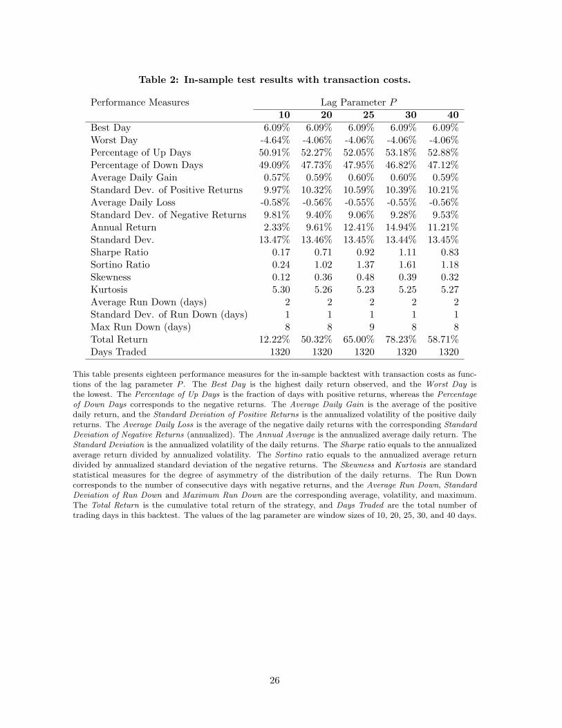
Table 2: In-sample test results with transaction costs.
Performance Measures Lag Parameter P10 20 25 30 40
Best Day 6.09% 6.09% 6.09% 6.09% 6.09%Worst Day -4.64% -4.06% -4.06% -4.06% -4.06%Percentage of Up Days 50.91% 52.27% 52.05% 53.18% 52.88%Percentage of Down Days 49.09% 47.73% 47.95% 46.82% 47.12%Average Daily Gain 0.57% 0.59% 0.60% 0.60% 0.59%Standard Dev. of Positive Returns 9.97% 10.32% 10.59% 10.39% 10.21%Average Daily Loss -0.58% -0.56% -0.55% -0.55% -0.56%Standard Dev. of Negative Returns 9.81% 9.40% 9.06% 9.28% 9.53%Annual Return 2.33% 9.61% 12.41% 14.94% 11.21%Standard Dev. 13.47% 13.46% 13.45% 13.44% 13.45%Sharpe Ratio 0.17 0.71 0.92 1.11 0.83Sortino Ratio 0.24 1.02 1.37 1.61 1.18Skewness 0.12 0.36 0.48 0.39 0.32Kurtosis 5.30 5.26 5.23 5.25 5.27Average Run Down (days) 2 2 2 2 2Standard Dev. of Run Down (days) 1 1 1 1 1Max Run Down (days) 8 8 9 8 8Total Return 12.22% 50.32% 65.00% 78.23% 58.71%Days Traded 1320 1320 1320 1320 1320
This table presents eighteen performance measures for the in-sample backtest with transaction costs as func-tions of the lag parameter P . The Best Day is the highest daily return observed, and the Worst Day isthe lowest. The Percentage of Up Days is the fraction of days with positive returns, whereas the Percentageof Down Days corresponds to the negative returns. The Average Daily Gain is the average of the positivedaily return, and the Standard Deviation of Positive Returns is the annualized volatility of the positive dailyreturns. The Average Daily Loss is the average of the negative daily returns with the corresponding StandardDeviation of Negative Returns (annualized). The Annual Average is the annualized average daily return. TheStandard Deviation is the annualized volatility of the daily returns. The Sharpe ratio equals to the annualizedaverage return divided by annualized volatility. The Sortino ratio equals to the annualized average returndivided by annualized standard deviation of the negative returns. The Skewness and Kurtosis are standardstatistical measures for the degree of asymmetry of the distribution of the daily returns. The Run Downcorresponds to the number of consecutive days with negative returns, and the Average Run Down, StandardDeviation of Run Down and Maximum Run Down are the corresponding average, volatility, and maximum.The Total Return is the cumulative total return of the strategy, and Days Traded are the total number oftrading days in this backtest. The values of the lag parameter are window sizes of 10, 20, 25, 30, and 40 days.
26

Table 3: Correlations between the strategy in-sample returns and the individualindexes.
AEX CAC DAX FTSE StrategyAEX 1.00CAC 0.94 1.00DAX 0.84 0.87 1.00
FTSE 0.85 0.86 0.75 1.00Strategy -0.06 -0.04 -0.01 -0.04 1.00
This table presents the correlations of the daily returns of the four indexes (AEX, CAC, DAX and FTSE),and the daily returns of the trading strategy (in-sample backtest) without transaction costs.
27

Table 4: Out-of-sample test without transaction cost, sliding window size 1000days.
Performance Measures Lag Parameter P10 20 25 30 40
Best Day 3.77% 3.77% 3.84% 3.84% 3.84%Worst Day -4.05% -4.05% -4.05% -4.05% -4.05%Percentage of Up Days 50.91% 52.73% 53.26% 52.42% 50.91%Percentage of Down Days 49.09% 47.27% 46.74% 47.58% 49.09%Average Daily Gain 0.48% 0.50% 0.52% 0.51% 0.49%Standard Dev. of Positive Returns 7.46% 7.59% 7.99% 7.61% 7.51%Average Daily Loss -0.49% -0.47% -0.45% -0.46% -0.49%Standard Dev. of Negative Returns 7.87% 7.75% 7.23% 7.70% 7.82%Annual Return 2.00% 9.67% 16.31% 11.62% 2.21%Standard Dev. 10.87% 10.86% 10.82% 10.85% 10.87%Sharpe Ratio 0.18 0.89 1.51 1.07 0.20Sortino Ratio 0.25 1.25 2.26 1.51 0.28Skewness -0.14 -0.12 0.20 -0.13 -0.15Kurtosis 4.34 4.38 4.33 4.40 4.34Average Run Down (days) 2 2 2 2 2Standard Dev. of Run Down (days) 1 1 1 1 1Max Run Down (days) 9 7 7 8 10Total Return 10.50% 50.67% 85.45% 60.86% 11.57%Days Traded 1320 1320 1320 1320 1320
This table presents eighteen performance measures for the out-of-sample backtest with sliding window sizeof 1000, without transaction costs, as functions of the lag parameter P . The Best Day is the highest dailyreturn observed, and the Worst Day is the lowest. The Percentage of Up Days is the fraction of days withpositive returns, whereas the Percentage of Down Days corresponds to the negative returns. The AverageDaily Gain is the average of the positive daily return, and the Standard Deviation of Positive Returns is theannualized volatility of the positive daily returns. The Average Daily Loss is the average of the negative dailyreturns with the corresponding Standard Deviation of Negative Returns (annualized). The Annual Average isthe annualized average daily return. The Standard Deviation is the annualized volatility of the daily returns.The Sharpe ratio equals to the annualized average return divided by annualized volatility. The Sortino ratioequals to the annualized average return divided by annualized standard deviation of the negative returns. TheSkewness and Kurtosis are standard statistical measures for the degree of asymmetry of the distribution ofthe daily returns. The Run Down corresponds to the number of consecutive days with negative returns, andthe Average Run Down, Standard Deviation of Run Down and Maximum Run Down are the correspondingaverage, volatility, and maximum. The Total Return is the cumulative total return of the strategy, and DaysTraded are the total number of trading days in this backtest. The values of the lag parameter are windowsizes of 10, 20, 25, 30, and 40 days.
28

Table 5: Out-of-sample test without transaction costs, sliding window size 1250days.
Performance Measures Lag Parameter P10 20 25 30 40
Best Day 3.78% 3.78% 3.86% 3.86% 3.86%Worst Day -3.99% -3.99% -3.99% -3.99% -3.99%Percentage of Up Days 50.23% 52.65% 52.73% 52.65% 52.50%Percentage of Down Days 49.77% 47.35% 47.27% 47.35% 47.50%Average Daily Gain 0.48% 0.49% 0.50% 0.49% 0.47%Standard Dev. of Positive Returns 7.55% 7.50% 7.88% 7.50% 7.40%Average Daily Loss -0.46% -0.46% -0.44% -0.45% -0.47%Standard Dev. of Negative Returns 7.64% 7.68% 7.22% 7.69% 7.80%Annual Return 3.20% 10.07% 14.82% 10.38% 6.43%Standard Dev. 10.66% 10.64% 10.62% 10.64% 10.65%Sharpe Ratio 0.30 0.95 1.40 0.98 0.60Sortino Ratio 0.42 1.31 2.05 1.35 0.83Skewness -0.06 -0.11 0.21 -0.11 -0.15Kurtosis 4.74 4.79 4.73 4.80 4.77Average Run Down (days) 2 2 2 2 2Standard Dev. of Run Down (days) 1 1 1 1 1Max Run Down (days) 8 7 10 7 10Total Return 16.79% 52.76% 77.65% 54.38% 33.69%Days Traded 1320 1320 1320 1320 1320
This table presents eighteen performance measures for the out-of-sample backtest with sliding window size of1250 days, without transaction costs, as functions of the lag parameter P . The Best Day is the highest dailyreturn observed, and the Worst Day is the lowest. The Percentage of Up Days is the fraction of days withpositive returns, whereas the Percentage of Down Days corresponds to the negative returns. The AverageDaily Gain is the average of the positive daily return, and the Standard Deviation of Positive Returns is theannualized volatility of the positive daily returns. The Average Daily Loss is the average of the negative dailyreturns with the corresponding Standard Deviation of Negative Returns (annualized). The Annual Average isthe annualized average daily return. The Standard Deviation is the annualized volatility of the daily returns.The Sharpe ratio equals to the annualized average return divided by annualized volatility. The Sortino ratioequals to the annualized average return divided by annualized standard deviation of the negative returns. TheSkewness and Kurtosis are standard statistical measures for the degree of asymmetry of the distribution ofthe daily returns. The Run Down corresponds to the number of consecutive days with negative returns, andthe Average Run Down, Standard Deviation of Run Down and Maximum Run Down are the correspondingaverage, volatility, and maximum. The Total Return is the cumulative total return of the strategy, and DaysTraded are the total number of trading days in this backtest. The values of the lag parameter are windowsizes of 10, 20, 25, 30, and 40 days.
29
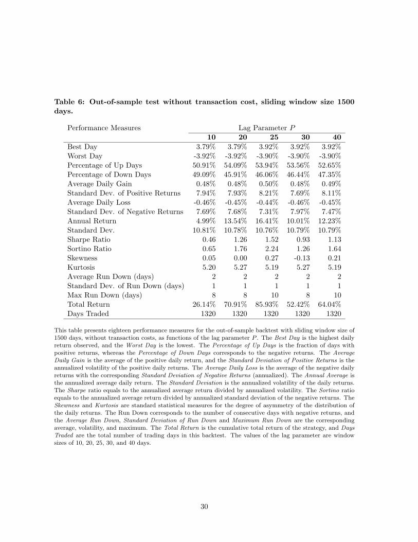
Table 6: Out-of-sample test without transaction cost, sliding window size 1500days.
Performance Measures Lag Parameter P10 20 25 30 40
Best Day 3.79% 3.79% 3.92% 3.92% 3.92%Worst Day -3.92% -3.92% -3.90% -3.90% -3.90%Percentage of Up Days 50.91% 54.09% 53.94% 53.56% 52.65%Percentage of Down Days 49.09% 45.91% 46.06% 46.44% 47.35%Average Daily Gain 0.48% 0.48% 0.50% 0.48% 0.49%Standard Dev. of Positive Returns 7.94% 7.93% 8.21% 7.69% 8.11%Average Daily Loss -0.46% -0.45% -0.44% -0.46% -0.45%Standard Dev. of Negative Returns 7.69% 7.68% 7.31% 7.97% 7.47%Annual Return 4.99% 13.54% 16.41% 10.01% 12.23%Standard Dev. 10.81% 10.78% 10.76% 10.79% 10.79%Sharpe Ratio 0.46 1.26 1.52 0.93 1.13Sortino Ratio 0.65 1.76 2.24 1.26 1.64Skewness 0.05 0.00 0.27 -0.13 0.21Kurtosis 5.20 5.27 5.19 5.27 5.19Average Run Down (days) 2 2 2 2 2Standard Dev. of Run Down (days) 1 1 1 1 1Max Run Down (days) 8 8 10 8 10Total Return 26.14% 70.91% 85.93% 52.42% 64.04%Days Traded 1320 1320 1320 1320 1320
This table presents eighteen performance measures for the out-of-sample backtest with sliding window size of1500 days, without transaction costs, as functions of the lag parameter P . The Best Day is the highest dailyreturn observed, and the Worst Day is the lowest. The Percentage of Up Days is the fraction of days withpositive returns, whereas the Percentage of Down Days corresponds to the negative returns. The AverageDaily Gain is the average of the positive daily return, and the Standard Deviation of Positive Returns is theannualized volatility of the positive daily returns. The Average Daily Loss is the average of the negative dailyreturns with the corresponding Standard Deviation of Negative Returns (annualized). The Annual Average isthe annualized average daily return. The Standard Deviation is the annualized volatility of the daily returns.The Sharpe ratio equals to the annualized average return divided by annualized volatility. The Sortino ratioequals to the annualized average return divided by annualized standard deviation of the negative returns. TheSkewness and Kurtosis are standard statistical measures for the degree of asymmetry of the distribution ofthe daily returns. The Run Down corresponds to the number of consecutive days with negative returns, andthe Average Run Down, Standard Deviation of Run Down and Maximum Run Down are the correspondingaverage, volatility, and maximum. The Total Return is the cumulative total return of the strategy, and DaysTraded are the total number of trading days in this backtest. The values of the lag parameter are windowsizes of 10, 20, 25, 30, and 40 days.
30

Table 7: Correlations between the strategy out-of-sample returns and the indi-vidual indexes.
AEX CAC DAX FTSE StrategyAEX 1.00CAC 0.94 1.00DAX 0.84 0.87 1.00
FTSE 0.85 0.86 0.75 1.00Strategy -0.02 -0.03 0.01 -0.04 1.00
This table presents the correlations of the daily returns of the four indexes (AEX, CAC, DAX and FTSE),and the daily returns of the trading strategy out-of-sample backtest, lag parameter of 25 and window size1000 days, without transaction costs.
31

Table 8: Out-of-sample test without transaction cost, cumulative window, start-ing with window size 1000 days.
Performance Measures Lag Parameter P10 20 25 30 40
Best Day 3.80% 3.80% 3.88% 3.88% 3.88%Worst Day -4.03% -4.03% -4.03% -4.03% -4.03%Percentage of Up Days 50.30% 52.12% 52.65% 53.11% 51.52%Percentage of Down Days 49.70% 47.88% 47.35% 46.89% 48.48%Average Daily Gain 0.47% 0.47% 0.49% 0.47% 0.46%Standard Dev. of Positive Returns 7.41% 7.44% 7.89% 7.42% 7.46%Average Daily Loss -0.45% -0.45% -0.43% -0.45% -0.46%Standard Dev. of Negative Returns 7.71% 7.69% 7.15% 7.72% 7.68%Annual Return 3.36% 8.51% 14.13% 10.49% 4.56%Standard Dev. 10.52% 10.51% 10.49% 10.50% 10.52%Sharpe Ratio 0.32 0.81 1.35 1.00 0.43Sortino Ratio 0.44 1.11 1.98 1.36 0.59Skewness -0.14 -0.15 0.22 -0.17 -0.10Kurtosis 5.13 5.17 5.11 5.20 5.13Average Run Down (days) 2 2 2 2 2Standard Dev. of Run Down (days) 1 1 1 1 1Max Run Down (days) 8 9 8 8 8Total Return 17.59% 44.57% 74.01% 54.95% 23.89%Days Traded 1320 1320 1320 1320 1320
This table presents eighteen performance measures for the out-of-sample backtest, cumulative window, startingwith window size 1000 days, without transaction costs, as functions of the lag parameter P . The Best Day isthe highest daily return observed, and the Worst Day is the lowest. The Percentage of Up Days is the fractionof days with positive returns, whereas the Percentage of Down Days corresponds to the negative returns.The Average Daily Gain is the average of the positive daily return, and the Standard Deviation of PositiveReturns is the annualized volatility of the positive daily returns. The Average Daily Loss is the average ofthe negative daily returns with the corresponding Standard Deviation of Negative Returns (annualized). TheAnnual Average is the annualized average daily return. The Standard Deviation is the annualized volatility ofthe daily returns. The Sharpe ratio equals to the annualized average return divided by annualized volatility.The Sortino ratio equals to the annualized average return divided by annualized standard deviation of thenegative returns. The Skewness and Kurtosis are standard statistical measures for the degree of asymmetryof the distribution of the daily returns. The Run Down corresponds to the number of consecutive days withnegative returns, and the Average Run Down, Standard Deviation of Run Down and Maximum Run Downare the corresponding average, volatility, and maximum. The Total Return is the cumulative total return ofthe strategy, and Days Traded are the total number of trading days in this backtest. The values of the lagparameter are window sizes of 10, 20, 25, 30, and 40 days.
32

Table 9: Out-of-sample test without transaction cost, cumulative window, start-ing with window size 1250 days.
Performance Measures Lag Parameter P10 20 25 30 40
Best Day 3.76% 3.76% 3.88% 3.88% 3.88%Worst Day -3.93% -3.93% -3.93% -3.93% -3.93%Percentage of Up Days 50.23% 53.64% 53.26% 52.88% 52.27%Percentage of Down Days 49.77% 46.36% 46.74% 47.12% 47.73%Average Daily Gain 0.49% 0.49% 0.50% 0.48% 0.48%Standard Dev. of Positive Returns 7.74% 7.67% 7.96% 7.46% 7.61%Average Daily Loss -0.46% -0.46% -0.45% -0.47% -0.47%Standard Dev. of Negative Returns 7.55% 7.61% 7.25% 7.85% 7.68%Annual Return 3.29% 12.97% 13.65% 8.33% 7.05%Standard Dev. 10.74% 10.71% 10.70% 10.73% 10.73%Sharpe Ratio 0.31 1.21 1.28 0.78 0.66Sortino Ratio 0.44 1.70 1.88 1.06 0.92Skewness 0.05 -0.07 0.22 -0.17 -0.06Kurtosis 4.91 4.99 4.90 4.96 4.94Average Run Down (days) 2 2 2 2 2Standard Dev. of Run Down (days) 1 1 1 1 1Max Run Down (days) 8 7 7 7 7Total Return 17.22% 67.92% 71.51% 43.65% 36.94%Days Traded 1320 1320 1320 1320 1320
This table presents eighteen performance measures for the out-of-sample backtest, cumulative window, startingwith window size of 1250 days, without transaction costs, as functions of the lag parameter P . The Best Day isthe highest daily return observed, and the Worst Day is the lowest. The Percentage of Up Days is the fractionof days with positive returns, whereas the Percentage of Down Days corresponds to the negative returns.The Average Daily Gain is the average of the positive daily return, and the Standard Deviation of PositiveReturns is the annualized volatility of the positive daily returns. The Average Daily Loss is the average ofthe negative daily returns with the corresponding Standard Deviation of Negative Returns (annualized). TheAnnual Average is the annualized average daily return. The Standard Deviation is the annualized volatility ofthe daily returns. The Sharpe ratio equals to the annualized average return divided by annualized volatility.The Sortino ratio equals to the annualized average return divided by annualized standard deviation of thenegative returns. The Skewness and Kurtosis are standard statistical measures for the degree of asymmetryof the distribution of the daily returns. The Run Down corresponds to the number of consecutive days withnegative returns, and the Average Run Down, Standard Deviation of Run Down and Maximum Run Downare the corresponding average, volatility, and maximum. The Total Return is the cumulative total return ofthe strategy, and Days Traded are the total number of trading days in this backtest. The values of the lagparameter are window sizes of 10, 20, 25, 30, and 40 days.
33

Table 10: Out-of-sample test without transaction cost, cumulative window, star-ing with window size 1500 days.
Performance Measures Lag Parameter P10 20 25 30 40
Best Day 3.91% 4.07% 4.07% 4.07% 4.07%Worst Day -4.37% -4.37% -4.37% -4.37% -4.37%Percentage of Up Days 49.92% 52.80% 52.88% 53.18% 51.97%Percentage of Down Days 50.08% 47.20% 47.12% 46.82% 48.03%Average Daily Gain 0.50% 0.51% 0.52% 0.50% 0.52%Standard Dev. of Positive Returns 7.92% 8.32% 8.42% 8.19% 8.68%Average Daily Loss -0.49% -0.47% -0.46% -0.47% -0.46%Standard Dev. of Negative Returns 8.30% 7.85% 7.71% 8.01% 7.41%Annual Return 1.09% 12.23% 14.43% 11.42% 12.71%Standard Dev. 11.24% 11.21% 11.20% 11.21% 11.21%Sharpe Ratio 0.10 1.09 1.29 1.02 1.13Sortino Ratio 0.13 1.56 1.87 1.43 1.72Skewness -0.17 0.13 0.17 0.03 0.39Kurtosis 5.20 5.21 5.21 5.23 5.13Average Run Down (days) 2 2 2 2 2Standard Dev. of Run Down (days) 1 1 1 1 1Max Run Down (days) 8 8 8 8 8Total Return 5.70% 64.05% 75.61% 59.82% 66.57%Days Traded 1320 1320 1320 1320 1320
This table presents eighteen performance measures for the out-of-sample backtest, cumulative window, startingwith window size of 1500 days, without transaction costs, as functions of the lag parameter P . The Best Day isthe highest daily return observed, and the Worst Day is the lowest. The Percentage of Up Days is the fractionof days with positive returns, whereas the Percentage of Down Days corresponds to the negative returns.The Average Daily Gain is the average of the positive daily return, and the Standard Deviation of PositiveReturns is the annualized volatility of the positive daily returns. The Average Daily Loss is the average ofthe negative daily returns with the corresponding Standard Deviation of Negative Returns (annualized). TheAnnual Average is the annualized average daily return. The Standard Deviation is the annualized volatility ofthe daily returns. The Sharpe ratio equals to the annualized average return divided by annualized volatility.The Sortino ratio equals to the annualized average return divided by annualized standard deviation of thenegative returns. The Skewness and Kurtosis are standard statistical measures for the degree of asymmetryof the distribution of the daily returns. The Run Down corresponds to the number of consecutive days withnegative returns, and the Average Run Down, Standard Deviation of Run Down and Maximum Run Downare the corresponding average, volatility, and maximum. The Total Return is the cumulative total return ofthe strategy, and Days Traded are the total number of trading days in this backtest. The values of the lagparameter are window sizes of 10, 20, 25, 30, and 40 days.
34
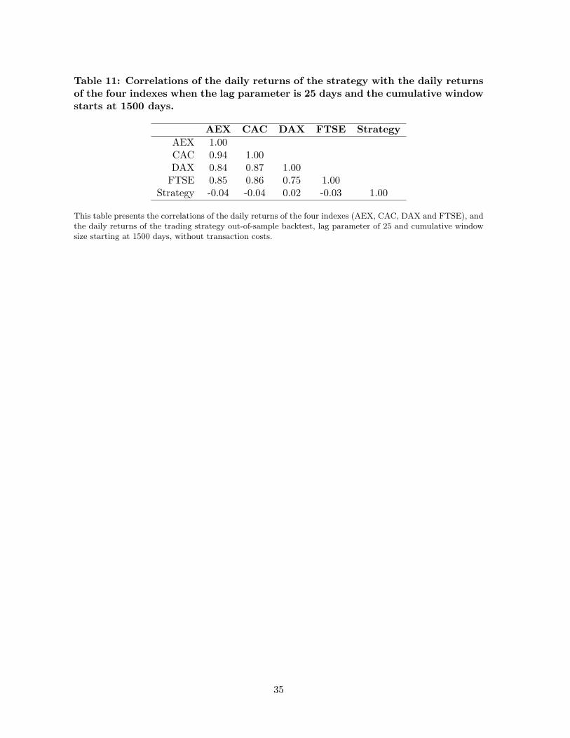
Table 11: Correlations of the daily returns of the strategy with the daily returnsof the four indexes when the lag parameter is 25 days and the cumulative windowstarts at 1500 days.
AEX CAC DAX FTSE StrategyAEX 1.00CAC 0.94 1.00DAX 0.84 0.87 1.00
FTSE 0.85 0.86 0.75 1.00Strategy -0.04 -0.04 0.02 -0.03 1.00
This table presents the correlations of the daily returns of the four indexes (AEX, CAC, DAX and FTSE), andthe daily returns of the trading strategy out-of-sample backtest, lag parameter of 25 and cumulative windowsize starting at 1500 days, without transaction costs.
35

Figures
Figure 1: Total return for the in-sample backtest vs the four indexes.
-1
-0.8
-0.6
-0.4
-0.2
0
0.2
0.4
0.6
0.8
1
11/7
/200
1
1/7/
2002
3/7/
2002
5/7/
2002
7/7/
2002
9/7/
2002
11/7
/200
2
1/7/
2003
3/7/
2003
5/7/
2003
7/7/
2003
9/7/
2003
11/7
/200
3
1/7/
2004
3/7/
2004
5/7/
2004
7/7/
2004
9/7/
2004
11/7
/200
4
1/7/
2005
3/7/
2005
5/7/
2005
7/7/
2005
9/7/
2005
11/7
/200
5
1/7/
2006
3/7/
2006
5/7/
2006
7/7/
2006
9/7/
2006
11/7
/200
6
AEX CAC DAX FTSE COINTEGRATION STRATEGY
This figure shows the dynamics of the cumulative returns from the in-sample backtest without transactioncosts, compared to the corresponding returns of the four indexes (AEX, CAC, DAX, FTSE). The horizontalaxis is the time, and the vertical axis is the total cumulative return.
36

Figure 2: Total return for out-of-sample test as a function of the lag parameter and windowsize, fixed case, no transaction costs.
This figure is a 3 dimensional plot of the total return of the cointegration daily strategy (out-of-sample test)as a function of the window size and the lag. The strategy was run using the following values of the windowsize 1000, 1250 and 1500; the values of the lag were 10,15,20,25,30,35 and 40.
37

Figure 3: Total return for out-of-sample aggregate test as a function of the lag parameterand window size, no transaction costs.
This figure is a 3 dimensional plot of the total return of the cointegration daily strategy (out-of-sampleaggregate test) as a function of the window size and the lag. The strategy was run using the following valuesof the window size 1000, 1250 and 1500; the values of the lag were 10,15,20,25,30,35 and 40.
38

Figure 4: Total return for the out-of-sample backtest (lag 25, window size 1000) vs the fourindexes.
-1
-0.8
-0.6
-0.4
-0.2
0
0.2
0.4
0.6
0.8
1
11/7
/200
1
1/7/
2002
3/7/
2002
5/7/
2002
7/7/
2002
9/7/
2002
11/7
/200
2
1/7/
2003
3/7/
2003
5/7/
2003
7/7/
2003
9/7/
2003
11/7
/200
3
1/7/
2004
3/7/
2004
5/7/
2004
7/7/
2004
9/7/
2004
11/7
/200
4
1/7/
2005
3/7/
2005
5/7/
2005
7/7/
2005
9/7/
2005
11/7
/200
5
1/7/
2006
3/7/
2006
5/7/
2006
7/7/
2006
9/7/
2006
11/7
/200
6
AEX CAC DAX FTSE Strategy
This figure shows the dynamics of the cumulative returns from the out-of-sample backtest done with a lag of25 days and a window size of 1000 days without transaction costs, compared to the corresponding returns ofthe four indexes (AEX, CAC, DAX, FTSE). The horizontal axis is the time, and the vertical axis is the totalcumulative return.
39

Figure 5: Time plot of the estimated cointegration vector.
-80
-60
-40
-20
0
20
40
60
11/6
/200
1
1/6/
2002
3/6/
2002
5/6/
2002
7/6/
2002
9/6/
2002
11/6
/200
2
1/6/
2003
3/6/
2003
5/6/
2003
7/6/
2003
9/6/
2003
11/6
/200
3
1/6/
2004
3/6/
2004
5/6/
2004
7/6/
2004
9/6/
2004
11/6
/200
4
1/6/
2005
3/6/
2005
5/6/
2005
7/6/
2005
9/6/
2005
11/6
/200
5
1/6/
2006
3/6/
2006
5/6/
2006
7/6/
2006
9/6/
2006
11/6
/200
6
AEX CAC DAX FTSE
This figure shows the estimated cointegration vector as a function of time. The vector is re-estimated every22 days using the Johansen cointegration rank test with data from the previous 1000 days.
40

Figure 6: Total return for the out-of-sample backtest (lag 25, cumulative window starting at1500) vs the four indexes.
-1.00000
-0.80000
-0.60000
-0.40000
-0.20000
0.00000
0.20000
0.40000
0.60000
0.80000
1.00000
11/7
/200
1
1/7/
2002
3/7/
2002
5/7/
2002
7/7/
2002
9/7/
2002
11/7
/200
2
1/7/
2003
3/7/
2003
5/7/
2003
7/7/
2003
9/7/
2003
11/7
/200
3
1/7/
2004
3/7/
2004
5/7/
2004
7/7/
2004
9/7/
2004
11/7
/200
4
1/7/
2005
3/7/
2005
5/7/
2005
7/7/
2005
9/7/
2005
11/7
/200
5
1/7/
2006
3/7/
2006
5/7/
2006
7/7/
2006
9/7/
2006
11/7
/200
6
AEX CAC DAX FTSE Strategy
This figure shows the dynamics of the cumulative returns from the out-of-sample backtest done with a lag of 25days and a cumulative window starting at 1500 days without transaction costs, compared to the correspondingreturns of the four indexes (AEX, CAC, DAX, FTSE.) The horizontal axis is the time, and the vertical axisis the total cumulative return.
41

Figure 7: Time plot of the estimated cointegration vector when the lag parameter is 25 days,and the cumulative window starts at 1500 days.
-30
-20
-10
0
10
20
30
40
11/6
/200
1
1/6/
2002
3/6/
2002
5/6/
2002
7/6/
2002
9/6/
2002
11/6
/200
2
1/6/
2003
3/6/
2003
5/6/
2003
7/6/
2003
9/6/
2003
11/6
/200
3
1/6/
2004
3/6/
2004
5/6/
2004
7/6/
2004
9/6/
2004
11/6
/200
4
1/6/
2005
3/6/
2005
5/6/
2005
7/6/
2005
9/6/
2005
11/6
/200
5
1/6/
2006
3/6/
2006
5/6/
2006
7/6/
2006
9/6/
2006
11/6
/200
6
AEX CAC DAX FTSE
This figure shows the estimated cointegration vector as a function of time. The vector is re-estimated every22 days using the Johansen cointegration rank test using all data up to the current time period
42
Recommended