Totally Integrated Power
Totally Integrated Power
siemens.com/tip-cs
Applications for power distribution
Energy transparency


Contents Energy transparency
1 Electricity market and energy transparency 4
2 Fundamentals and terminology of energy transparency 8
2.1 Data compression 9
2.2 Data selection 10
2.3 Operator control and monitoring 11
2.4 Evaluating and optimizing 13
2.5 Planning and forecasting 17
3 Measured value acquisition in the distribution grid and its importance in the electricity market 20
3.1 Measured quantities and characteristic parameters in the customer’s power system 22
3.2 Derivation from synthetic load curves 24
3.3 Forecasts and the electricity market 25
4 Operational performance and efficiency in electric power distribution 30
4.1 Operating performance of transformers 30
4.2 Operating performance of generators 32
4.3 Motor and assembly control and adjustment 33
4.4 Distributed generation of electric energy 34
5 Checklists 38
5.1 Checklist for measured quantities 38
5.2 “Graphics” checklist and “Tables” checklist 40
6 Hardware and software for measured value acquisition and analysis 42
7 Smart energy control for specific applications 48
7.1 Shopping centre 49
7.2 Data centre 50
7.3 Industrial plant 51
7.4 Supermarket 52
7.5 Distributed properties 53
8 Annex 56
8.1 Value ranges for energy consumption and
power demand 56
8.2 Abbreviations 62
8.3 Formula symbols 62
8.4 Bibliography 63

Energy transparency
The basis for efficient electric power distribution is appropriate planning combined with demand-ori-
ented dimensioning of products and systems. Customers and approval authorities increasingly focus
on operation-related energy consumption. And last but not least, contractors are required to comply
with standards concerning energy management (ISO 50001) and energy efficiency (IEC 60364-8-1;
VDE 0100-801).
Without a comprehensive understanding of the energetic correlations which define energy transpar-
ency, there is no basis for operational efficiency evaluations and for energy management. So it is
imperative to provide for measurement and analysis of the electric power distribution system during
planning. In this context it is useful to distinguish between
• Power sources (such as transformers and generators)
• Connecting lines (such as cables and wires, busbar trunking systems)
• Protection and switching systems (such as switches, circuit-breakers, contactors, fuses)
• Loads (such as luminaires, frequency inverters, motors, pumps, power supply units)
Measuring instruments, data storage media, and a suitable analysis system (hardware and software)
are important aids which must be smartly employed as to attain the level of energy transparency
required in normal operation. The following might contribute to achieving this goal:
• Data acquisition of power consumption
• Utilization profile over time
• Voltage quality for power consuming equipment and load interference on the supply grid
• Comparisons of actual and target values
• Signalling (for example by warnings and alarms)
Therefore, integration of modern instrumentation should be a constituent part of planning, and the
resulting energy transparency can provide the plant with an additional competitive edge. This applica-
tion manual explains characteristic terminology, describes the structural design of a task-specific meas-
urement system, introduces and compares typical features of measuring instruments, and demon-
strates their use in a number of examples for various applications.

Chapter 1 Electricity market and energy transparency
4 Totally Integrated Power – Electricity market and energy transparency
1
1 Electricity market and energy transparency
Economic efficiency plays a particularly important role in
the commercial use of buildings. Recently it has become
apparent that operational energy costs are a significant
cost factor (Fig. 1/1). Cost reductions have become possible
in the liberalized electricity market thanks to aggressive
corporate procurement management. As a result of the
energy turnaround which is accompanied by an increasing
use of renewable energy sources whose availability
depends on greatly varying environmental conditions, the
availability of the commodity 'electricity' has tended to be
more incalculable so that the interplay of electricity supply
and electricity consumption is becoming increasingly
important.
In the future, favourable purchase conditions for electricity
will increasingly depend on the predictability and flexibility
of consumption. In the electricity supply contract between
consumer and electricity supplier, the different compo-
nents of electricity consumption such as base peak and
offpeak as a function of time blocks (Fig. 1/2) are
stipulated:
• Base: continuous electricity consumption for one day; for
a year the individual base day values may be specified
(one unit corresponds to 24 MWh/d)
• Peak: daily electricity consumption between 8 a. m. and
8 p. m. (one unit corresponds to 12 MWh/d)
• Offpeak: Electricity consumption of 1 MWh for one hour
at any time
Fig. 1/1: Cost of operation and investment for some building types
600
500
400
300
200
100
0 10 20 30 40 50
Total Cost in %
Hospitals
Indoor swimming pools
Production facilities
Residential buildings
Investment
Office buildings
Years
Usa
ge
Re
a-
liza
-ti
on
Planning today: Low investmentPlanning tomorrow: Efficient operation focussing on operating costs
The electricity cost contributes to the costs of materials or operation to an extent that should not be neglected, such as:office building: approx. 10 to 12 % according to [1.1]hospital: approx. 3.5 % according to [1.2]
5Totally Integrated Power – Electricity market and energy transparency
1
Quarter-hour based purchase contracts of energy con-
sumers with an annual consumption of more than
100,000 kWh/a, may require demand forecasts on a
15 min basis. Time requirements and options for optimiza-
tion are diagrammatically compiled in Fig. 1/3.
Fig. 1/2: Contract modules in electricity trading
BaseContracted unit 24 MWh per day
PeakContracted unit 12 MWh per day
from 6:00 until 20:00
OffpeakContracted unit 1 MWh
6:00 12:00 18:00 24:000:00
Power
time
Fig. 1/3: Time schedule for forecast optimization and limit monitoring for meeting forecast volumes
11:00 11:05 11:10 11:15
100 %
60 %
140 %
20 %
0:15 12:15 24:0018:156:15- 50
150
100
50
0
kW
50
0
- 50
- 100
kW
50
0
- 50
- 100
kW
Thur SunSatFri
Previous week
Forecast and optimization under a quarter-hour purchase contract for commercial customers (above 100,000 kWh per year)
Quarterly-hours valuesStart: Mon 00:15End: Sun 24:00
Difference for quarter-hourly valuesStart: Tue 00:15End: Tue 24:00
Difference forquarter-hourly valuesStart: Tue 09:15End: Tue 10:00
On the Thursdayfor the next week
Energy forecast per week
Day
Forecast optimization per day
for the following day
Hour,quarter-hour
for the following hour
Forecast optimizationhour, quarter-hour
Tue FriThurWed Sat SunMon
Week
Measurement and power output adjust-ment in the quarter-hourly cycle
Forecast balancing in case of target-actual difference
Current electricity purchase curve (measurements taken every 10 seconds))
Mean value for electricity purchase up to the current time
Forecasted quarter-hour value for electricity purchase
Linear power change (as of the current time) until there is a constant power decrease to balance the quarter-hour forecast
TargetActual

6 Totally Integrated Power – Electricity market and energy transparency
1
For this purpose, the consumer must submit a quarter-hour
based forecast of his power demand to the electricity sup-
plier in advance. The forecast covering one week from
Monday through Sunday must be provided on the Thursday
of the previous week (Fig. 1/3). Forecast optimizations may,
however, be submitted for individual days, hours, and even
quarter-hours at the agreed times (following day, following
hour, ...) as diagrammatically shown in Fig. 1/3. This
involves the corresponding contractual stipulations.
Within the current quarter-hour, it is the consumer’s
responsibility to ensure compliance with the submitted
forecast by way of load management. In accordance with a
priority list set up by the consumer, loads are connected
into and disconnected from supply or controlled to balance
the difference between target and actual power. For extrap-
olations of the quarter-hour energy value, the forecast
must be checked at short intervals (typically 10 seconds)
(Fig. 1/3) and adjusted if necessary.
Continuous transparency of system operation is the prereq-
uisite for ensuring a long-term cost-efficient, safe, and reli-
able energy supply. Minimizing electric power consumption
by a use-related optimization at the planning stage and
when installing the system is a standard requirement which
has been postulated in IEC 60364-8-1 (VDE 0100-801).
Thus energy transparency ensures the efficiency of power
systems in a smart way enabling, as a result, the operation
of a smart grid.
If consumers generate electricity themselves, be it for their
own use or for feeding it back into the distribution grid,
then the consumer’s own power system becomes a “micro
grid”. In the Micro Grid an orderly or even an optimized
mode of operation is not feasible without reliable forecasts
of consumer-related power demand.
The flexibility inherent in the Micro Grid also allows trading
in electricity. If balancing power is made available to trans-
mission grid operators for a quarter-hour period, this may
− dependent on response time and market conditions − be
even remunerative for the power generating entity.
• Primary balancing power (PBP, primary control):
Immediate response,
100 % balancing power after 30 seconds
• Secondary balancing power (SBP, secondary control):
Initial response within 30 seconds,
100 % balancing power after 5 minutes
• Tertiary balancing power (TBP, tertiary control):
First response after 5 minutes,
100 % balancing power after 15 minutes
The balancing power market manages positive and nega-
tive balancing power volumes. The transmission grid opera-
tor requires these for his contractually stipulated system
power. At present, the transmission grid operator directly
accesses the generating units provided by the consumer.
Metering is done unit-related; load control is performed by
telecontrol.
Note: This access “from outside” creates a conflict of objec-
tives for the consumer. If the consumer wants to fulfil his
forecast as accurately as possible, what he needs is flexibil-
ity. If this flexibility is, however, needed to safeguard bal-
ancing power, voltage stabilization, or balancing group
loyalty (see chap. 3), this will be to the detriment of the
consumer’s forecast fulfilment.
Forecasts are increasingly becoming the main constituent
of optimization, both in terms of the purchasing and the
supply of electrical energy. Only when the consumer is
aware of his own demand of electricity and the grid condi-
tions, can power generation/power transformation and
power import into the Micro Grid be planned and optimally
used. The prerequisites for this transparency are measure-
ments and their evaluations as specified below.
Chapter 2Fundamentals and terminology of energy transparency
2.1 Data compression 9
2.2 Data selection 10
2.3 Operator control and monitoring 11
2.4 Evaluating and optimizing 13
2.5 Planning and forecasting 17
8 Totally Integrated Power – Fundamentals and terminology of energy transparency
2
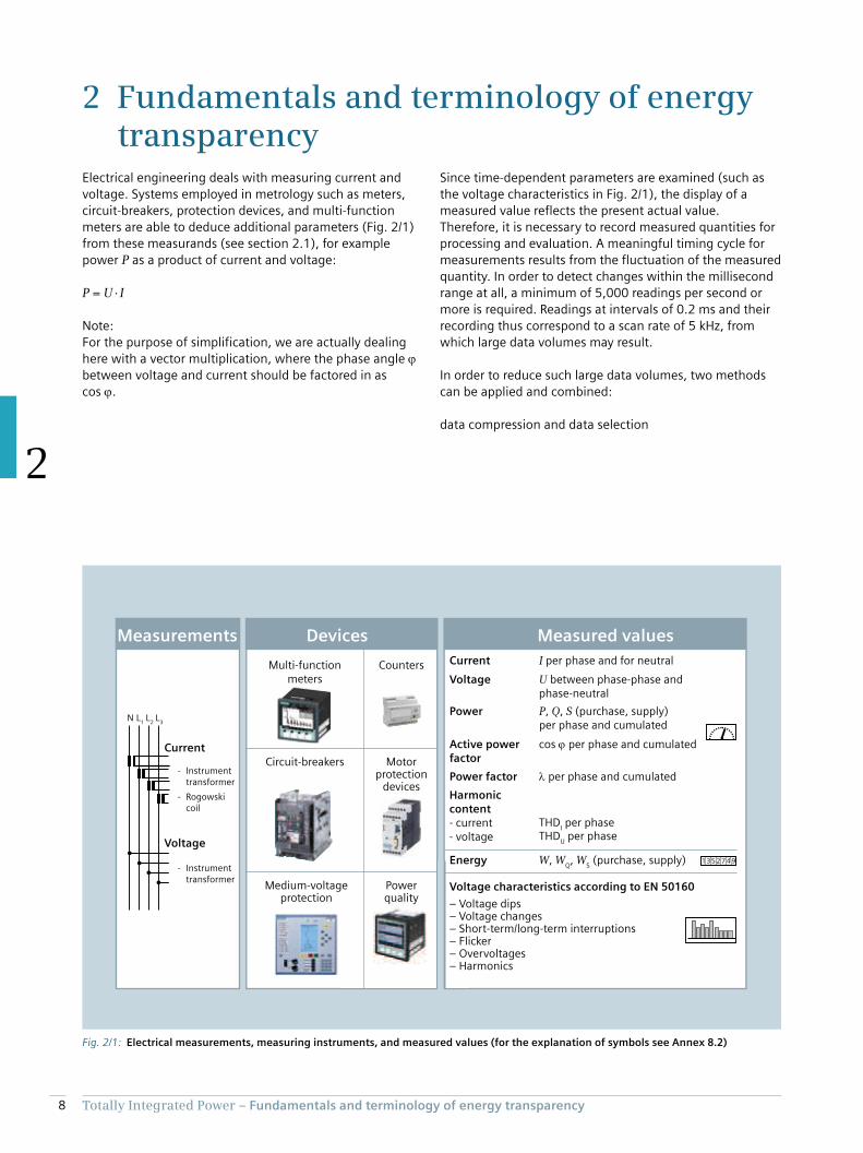
2 Fundamentals and terminology of energy transparency
Electrical engineering deals with measuring current and
voltage. Systems employed in metrology such as meters,
circuit-breakers, protection devices, and multi-function
meters are able to deduce additional parameters (Fig. 2/1)
from these measurands (see section 2.1), for example
power P as a product of current and voltage:
P = U · I
Note:
For the purpose of simplification, we are actually dealing
here with a vector multiplication, where the phase angle
between voltage and current should be factored in as
cos .
Since time-dependent parameters are examined (such as
the voltage characteristics in Fig. 2/1), the display of a
measured value reflects the present actual value.
Therefore, it is necessary to record measured quantities for
processing and evaluation. A meaningful timing cycle for
measurements results from the fluctuation of the measured
quantity. In order to detect changes within the millisecond
range at all, a minimum of 5,000 readings per second or
more is required. Readings at intervals of 0.2 ms and their
recording thus correspond to a scan rate of 5 kHz, from
which large data volumes may result.
In order to reduce such large data volumes, two methods
can be applied and combined:
data compression and data selection
Fig. 2/1: Electrical measurements, measuring instruments, and measured values (for the explanation of symbols see Annex 8.2)
L1
L2
L3
N
1352 7 49
Measurements Devices Measured values
Multi-functionmeters
Circuit-breakers
Counters
Motorprotection
devices
Medium-voltageprotection
Powerquality
Power
Energy
Current
Voltage
Voltage characteristics according to EN 50160
P, Q, S (purchase, supply)per phase and cumulated
W, WQ, W
S (purchase, supply)
– Voltage dips– Voltage changes– Short-term/long-term interruptions– Flicker– Overvoltages– Harmonics
Voltage
Current
- Instrument transformer
- Rogowski coil
- Instrument transformer
Power factor per phase and cumulated
I per phase and for neutral
U between phase-phase andphase-neutral
Active power factor
cos per phase and cumulated
Harmonic content- current- voltage
THDI per phase
THDU per phase
9Totally Integrated Power – Fundamentals and terminology of energy transparency
2
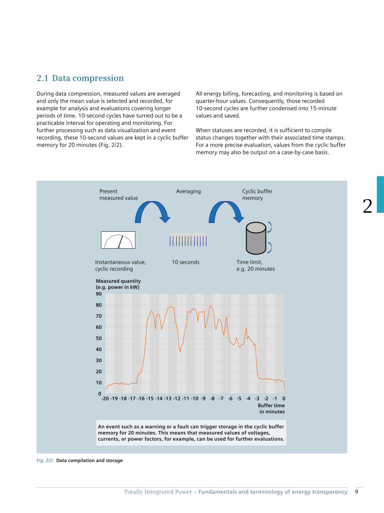
2.1 Data compression
During data compression, measured values are averaged
and only the mean value is selected and recorded, for
example for analysis and evaluations covering longer
periods of time. 10-second cycles have turned out to be a
practicable interval for operating and monitoring. For
further processing such as data visualization and event
recording, these 10-second values are kept in a cyclic buffer
memory for 20 minutes (Fig. 2/2).
All energy billing, forecasting, and monitoring is based on
quarter-hour values. Consequently, those recorded
10-second cycles are further condensed into 15-minute
values and saved.
When statuses are recorded, it is sufficient to compile
status changes together with their associated time stamps.
For a more precise evaluation, values from the cyclic buffer
memory may also be output on a case-by-case basis.
Fig. 2/2: Data compilation and storage
90
60
0
10
20
30
40
50
80
70
-20 -19 -18 -17 -16 -15 -14 -13 -12 -11 -10 -9 -8 -7 -6 -5 -4 -3 -2 -1 0
Buffer timein minutes
Measured quantity (e.g. power in kW)
Present measured value
Averaging
10 secondsInstantaneous value, cyclic recording
Cyclic buffer memory
Time limit, e.g. 20 minutes
An event such as a warning or a fault can trigger storage in the cyclic buffer memory for 20 minutes. This means that measured values of voltages, currents, or power factors, for example, can be used for further evaluations.
10 Totally Integrated Power – Fundamentals and terminology of energy transparency
2
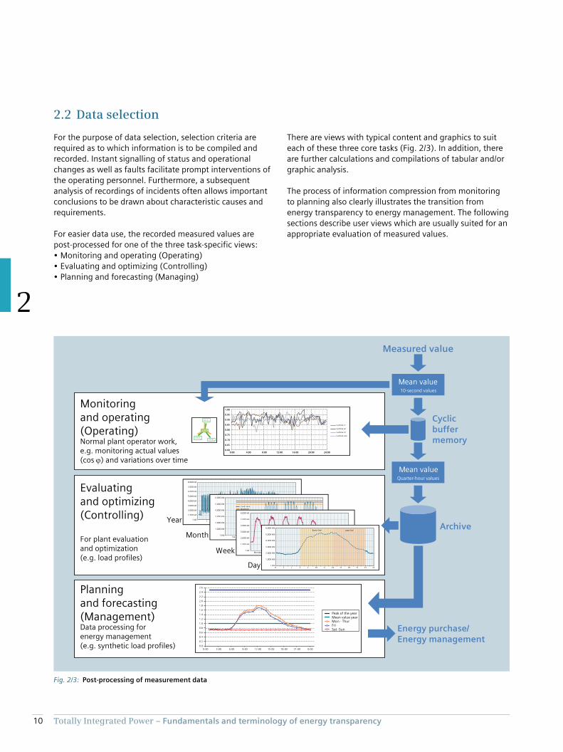
2.2 Data selection
For the purpose of data selection, selection criteria are
required as to which information is to be compiled and
recorded. Instant signalling of status and operational
changes as well as faults facilitate prompt interventions of
the operating personnel. Furthermore, a subsequent
analysis of recordings of incidents often allows important
conclusions to be drawn about characteristic causes and
requirements.
For easier data use, the recorded measured values are
post-processed for one of the three task-specific views:
• Monitoring and operating (Operating)
• Evaluating and optimizing (Controlling)
• Planning and forecasting (Managing)
There are views with typical content and graphics to suit
each of these three core tasks (Fig. 2/3). In addition, there
are further calculations and compilations of tabular and/or
graphic analysis.
The process of information compression from monitoring
to planning also clearly illustrates the transition from
energy transparency to energy management. The following
sections describe user views which are usually suited for an
appropriate evaluation of measured values.
Fig. 2/3: Post-processing of measurement data
0:00 3:00 6:00 9:00 12:00 15:00 18:00 21:00 0:00
cos L2
cos L1
cos L3
cos
8,000 kW
7,000 kW
6,000 kW
5,000 kW
4,000 kW
3,000 kW
2,000 kW
1,000 kW
1 kW1 5
Load curveLoad curLoad curLoad curveMaximumMaximumMaximumMaximum
6,000 kW
5,000 kW
4,000 kW
3,000 kW
2,000 kW
1,000 kW
1 kWCW 53
6,000 kW
5,000 kW
4,000 kW
3,000 kW
2,000 kW
1,000 kW
1 kWMonday
2 4 6 8 10 12 14 16 18 20 22 240
6,000 kW
5,000 kW
4,000 kW
3,000 kW
2,000 kW
1,000 kW
1 kW
Early ShiftEarEarly ShiftEarly Shiftly Shiftly Shift Late ShiftLatLatLate Shife Shife Shift
Planning and forecasting(Management) Data processing for energy management (e.g. synthetic load profiles)
Energy purchase/Energy management
Archive
Monitoring and operating(Operating)Normal plant operator work, e.g. monitoring actual values (cos ) and variations over time
Evaluating and optimizing(Controlling)
For plant evaluation and optimization (e.g. load profiles)
Cyclic buffer memory
Mean valueQuarter-hour values
Mean value10-second values
Year
Month
Week
Day
Peak of the yearMean value yearMon - Thur FriSat -Sun
0.0
1.8
2.6
2.4
2.2
2.0
1.6
1.4
1.2
1.0
0.8
0.6
0.4
0.60
0.95
0.90
0.85
0.80
0.75
0.70
0.65
1.00
0.2
Measured value
Lambda L1
Lambda L2
Lambda L3
Lambda sum
0:00 16:0012:008:004:00 20:00 24:00
11Totally Integrated Power – Fundamentals and terminology of energy transparency
2
2.3 Operator control and monitoring
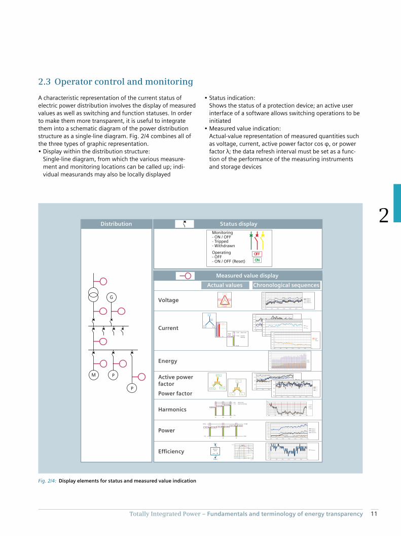
A characteristic representation of the current status of
electric power distribution involves the display of measured
values as well as switching and function statuses. In order
to make them more transparent, it is useful to integrate
them into a schematic diagram of the power distribution
structure as a single-line diagram. Fig. 2/4 combines all of
the three types of graphic representation.
• Display within the distribution structure:
Single-line diagram, from which the various measure-
ment and monitoring locations can be called up; indi-
vidual measurands may also be locally displayed
• Status indication:
Shows the status of a protection device; an active user
interface of a software allows switching operations to be
initiated
• Measured value indication:
Actual-value representation of measured quantities such
as voltage, current, active power factor cos φ, or power
factor λ; the data refresh interval must be set as a func-
tion of the performance of the measuring instruments
and storage devices
Fig. 2/4: Display elements for status and measured value indication
5 mA
0 mA
4 mA3,8 mA0 A
76 A Itherm
100 A Izul
108 A Imax
cos L2
cos L1
cos L3
cos
L2
L1
L3
8 %
0 %
7 %
5,58 %6,06 %
6,5 %
L1 L2 L3
110 kW
0 kW
100 %
0 %
81 % 89 kW76 % 83 kW
70 % 77 kW
L1 L2 L3
G
M P
P
OFF
ON
UL1-N
UL3-N UL2-NUL2-3
UL3-1 UL1-2
L1
L3 L2
N*
Energy L1
Energy L2
Energy L3
Energy Sum
0 kWh
1.000 kWh
900 kWh
800 kWh
700 kWh
600 kWh
500 kWh
400 kWh
300 kWh
200 kWh
100 kWh
23
:15
22
:15
21
:15
20
:15
19
:15
18
:15
17
:15
16
:15
15
:15
14
:15
13
:15
12
:15
11
:15
10
:15
9:1
5
8:1
5
7:1
5
6:1
5
5:1
5
4:1
5
3:1
5
2:1
5
1:1
5
23
:45
22
:45
21
:45
20
:45
19
:45
18
:45
17
:45
16
:45
15
:45
14
:45
13
:45
12
:45
11
:45
10
:45
9:4
5
8:4
5
7:4
5
6:4
5
5:4
5
4:4
5
3:4
5
2:4
5
1:4
5
0:4
5
0:1
5
0 A
0:00
Strom L1
Strom L2
Strom L3
Strom IN
0:00 20:0016:0012:008:004:00
100 A
80 A
120 A
60 A
40 A
20 A
0 A
0:00
IMAX
IZUL
Itherm
0:00 20:0016:0012:008:004:00
100 A
80 A
120 A
60 A
40 A
20 A
0 mA
0:00
Limit
Diff. current
0:00 20:0016:0012:008:004:00
5 mA
4 mA
6 mA
3 mA
2 mA
1 mA
0,60
0:00
cos L1
cos L2
cos L3
cos
0:00 20:0016:0012:008:004:00
0,90
0,80
0,70
1,00
0,60
0:00
L1
L2
L3
0:00 20:0016:0012:008:004:00
0,90
0,80
0,70
1,00
225 V
0:00
Voltage L1
Voltage L2
Voltage L3
Voltage sum
0:00 20:0016:0012:008:004:00
230 V
235 V
228 V
229 V
234 V
226 V
227 V
233 V
232 V
231 V
0 kW
0:000:00 20:0016:0012:008:004:00
50 kW
100 kW
30 kW
40 kW
90 kW
10 kW
20 kW
80 kW
70 kW
60 kW
0:000:00 20:0016:0012:008:004:00
322,5 kVA
Monitoring- ON / OFF- Tripped- Withdrawn
Operating- OFF- ON / OFF (Reset)
Distribution
Measured value display
Actual values Chronological sequences
Status display
Power in kVA
Efficiency in %
Power L1
Power L2
Power L3
Power Sum
0.80
Efficiency0.90
1.00
0.86
0.88
0.98
0.82
0.84
0.96
0.94
0.92
Limit forwarning
Alarm limitActualvalue
Limit for warning
Alarm limit
Input
... kW
Machinename
= ... %
... kW
Output
257,5 kVA -20 %
290 kVA -10 %
optimal work point
355 kVA +10 %
387,5 kVA +20 %
Voltage
Current
Energy
Active powerfactor
Power factor
Harmonics
Power
Efficiency
0 %
2 %
4 %
6 %
8 %
1 %
3 %
5 %
7 %
9 %
10 %
0:00 4:00 8:00 12:00 16:00 20:00 0:00
THD L1
EN50160
THD L2
THD L3
12 Totally Integrated Power – Fundamentals and terminology of energy transparency
2
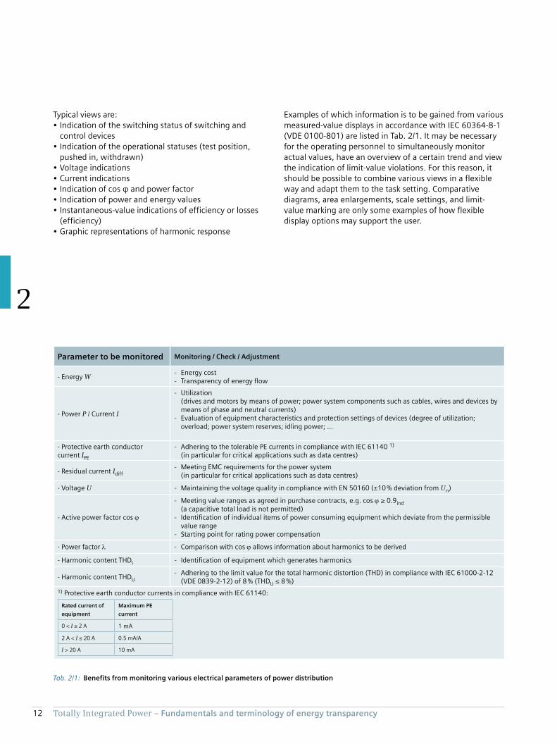
Typical views are:
• Indication of the switching status of switching and
control devices
• Indication of the operational statuses (test position,
pushed in, withdrawn)
• Voltage indications
• Current indications
• Indication of cos φ and power factor
• Indication of power and energy values
• Instantaneous-value indications of efficiency or losses
(efficiency)
• Graphic representations of harmonic response
Examples of which information is to be gained from various
measured-value displays in accordance with IEC 60364-8-1
(VDE 0100-801) are listed in Tab. 2/1. It may be necessary
for the operating personnel to simultaneously monitor
actual values, have an overview of a certain trend and view
the indication of limit-value violations. For this reason, it
should be possible to combine various views in a flexible
way and adapt them to the task setting. Comparative
diagrams, area enlargements, scale settings, and limit-
value marking are only some examples of how flexible
display options may support the user.
Tab. 2/1: Benefits from monitoring various electrical parameters of power distribution
Parameter to be monitored Monitoring / Check / Adjustment
- Energy W- Energy cost- Transparency of energy flow
- Power P / Current I
- Utilization (drives and motors by means of power; power system components such as cables, wires and devices by means of phase and neutral currents)- Evaluation of equipment characteristics and protection settings of devices (degree of utilization; overload; power system reserves; idling power; ...
- Protective earth conductor current IPE
- Adhering to the tolerable PE currents in compliance with IEC 61140 1) (in particular for critical applications such as data centres)
- Residual current Idiff- Meeting EMC requirements for the power system (in particular for critical applications such as data centres)
- Voltage U - Maintaining the voltage quality in compliance with EN 50160 (±10 % deviation from Un)
- Active power factor cos
- Meeting value ranges as agreed in purchase contracts, e.g. cos ≥ 0.9ind (a capacitive total load is not permitted)- Identification of individual items of power consuming equipment which deviate from the permissible value range- Starting point for rating power compensation
- Power factor - Comparison with cos allows information about harmonics to be derived
- Harmonic content THDI - Identification of equipment which generates harmonics
- Harmonic content THDU- Adhering to the limit value for the total harmonic distortion (THD) in compliance with IEC 61000-2-12 (VDE 0839-2-12) of 8 % (THDU ≤ 8 %)
1) Protective earth conductor currents in compliance with IEC 61140:
Rated current of
equipment
Maximum PE
current
0 < I ≤ 2 A 1 mA
2 A < I ≤ 20 A 0.5 mA/A
I > 20 A 10 mA
13Totally Integrated Power – Fundamentals and terminology of energy transparency
2
2.4 Evaluating and Optimizing
Whereas momentary time profiles are only displayed to
give up-to-date information for plant operation, longer
periods intended for evaluation are displayed as graphs or
bar diagrams. A compilation of characteristics in tabular
form may also help the assessment. The objective of evalu-
ation to be demonstrated is important for the choice of
view or for the compilation of characteristic parameters:
conditional upon, for example, the weekday, holiday times,
shift periods, seasonal weather conditions, and so on.
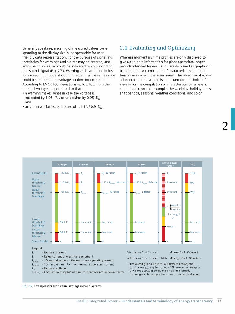
Generally speaking, a scaling of measured values corre-
sponding to the display size is indispensable for user-
friendly data representation. For the purpose of signalling,
thresholds for warnings and alarms may be entered, and
limits being exceeded could be indicated by colour-coding
or a sound signal (Fig. 2/5). Warning and alarm thresholds
for exceeding or undershooting the permissible value range
could be entered in the voltage section, for example.
According to EN 50160, deviations up to ±10 % from the
nominal voltage are permitted so that
• a warning makes sense in case the voltage is
exceeded by 1.05 · Un / or undershot by 0.95 · Un
and
• an alarm will be issued in case of 1.1 · Un / 0.9 · Un .
Fig. 2/5: Examples for limit value settings in bar diagrams
End of scale
Upperthreshold 2(alarm)
Lower threshold 2(alarm)
Upperthreshold 1(warning)
Lower threshold 1(warning)
Start of scale 0
10 %
8 %
irrelevant
irrelevant
0 %
7 %
Legend:
In = Nominal current
Ir = Rated current of electrical equipment
Ib, max
= 10-second value for the maximum operating current
Ib, mean
= 15-minute mean for the maximum operating current
Un = Nominal voltage
cos V = Contractually agreed minimum inductive active power factor
105 % Un
110 % Un
120 % Un
0
Ib, max
Ir
In
Ib, mean
· W-factor
110 % Ib, mean
· W-factor
In · W-factor
irrelevant
irrelevant
0
irrelevant
irrelevant90 % Un
95 % Un
0
irrelevant
1
irrelevant
0
1 + cos V
1)
2
cos V
1)
Ib, max
· P-factor
110 % Ib, max
· P-factor
In · P-factor
0
irrelevant
irrelevant
P-factor = 3 · Un · cos (Power P = I · P-factor)
W-factor = 3 · Un · cos · 1/4 h (Energy W = I · W-factor)
1) The warning is issued if cos is between cos v and
½ · (1 + cos v), e.g. for cos
v = 0.9 the warning range is
0.9 ≤ cos ≤ 0.95; below this an alarm is issued, meaning also for a capacitive cos (cross-hatched area)
Voltage CurrentActive power
factorTHD
UEnergy Power
capacitive
inductive
14 Totally Integrated Power – Fundamentals and terminology of energy transparency
2
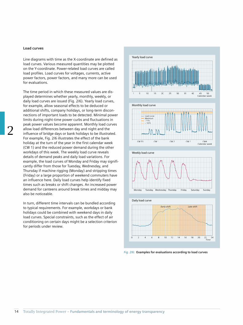
Load curves
Line diagrams with time as the X-coordinate are defined as
load curves. Various measured quantities may be plotted
on the Y-coordinate. Power-related load curves are called
load profiles. Load curves for voltages, currents, active
power factors, power factors, and many more can be used
for evaluations.
The time period in which these measured values are dis-
played determines whether yearly, monthly, weekly, or
daily load curves are issued (Fig. 2/6). Yearly load curves,
for example, allow seasonal effects to be deduced or
additional shifts, company holidays, or long-term discon-
nections of important loads to be detected. Minimal power
limits during night-time power curbs and fluctuations in
peak power values become apparent. Monthly load curves
allow load differences between day and night and the
influence of bridge days or bank holidays to be illustrated.
For example, Fig. 2/6 illustrates the effect of the bank
holiday at the turn of the year in the first calendar week
(CW 1) and the reduced power demand during the other
workdays of this week. The weekly load curve reveals
details of demand peaks and daily load variations. For
example, the load curves of Monday and Friday may signifi-
cantly differ from those for Tuesday, Wednesday, and
Thursday if machine rigging (Monday) and stripping times
(Friday) or a large proportion of weekend commuters have
an influence here. Daily load curves help identify fixed
times such as breaks or shift changes. An increased power
demand for canteens around break times and midday may
also be noticeable.
In turn, different time intervals can be bundled according
to typical requirements. For example, workdays or bank
holidays could be combined with weekend days in daily
load curves. Special constraints, such as the effect of air
conditioning on certain days might be a selection criterion
for periods under review.
Fig. 2/6: Examples for evaluations according to load curves
2 4 6 8 10 12 14 16 18 20 22 240
Load curveLoad curLoad curLoad curLoad curveMaximumMaximumMaximumMaximumMaximum– 5 %– 5 %– 5 %– 10 %– 10 %– 10 %– 10 %
CW 53 CW 1 CW 2 CW 3 CW4
Monday Tuesday Wednesday Thursday Friday Saturday Sunday
Early shiftEarEarly shiftEarly shiftly shiftly shift Late shiftLatLate shifLate shife shife shif
Daily load curve
Weekly load curve
Monthly load curve
Yearly load curve
Calendar week
Calendar week
Time
1 5 10 15 20 25 30 35 40 45 50
15Totally Integrated Power – Fundamentals and terminology of energy transparency
2
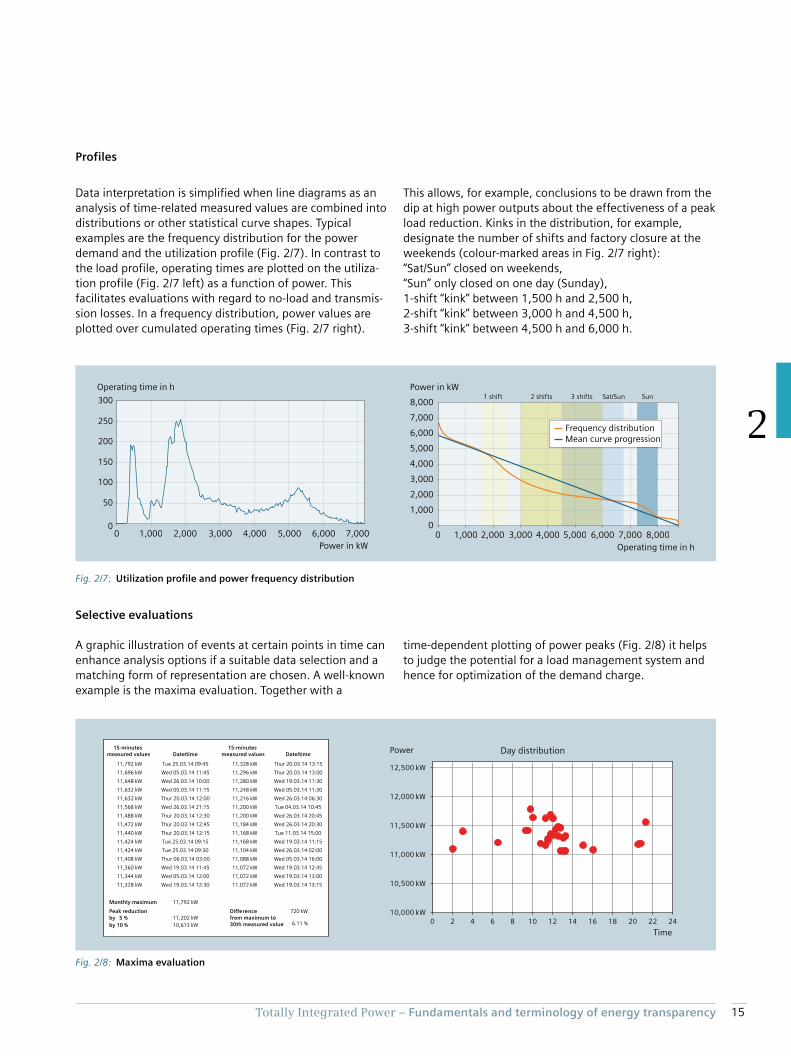
Profiles
Data interpretation is simplified when line diagrams as an
analysis of time-related measured values are combined into
distributions or other statistical curve shapes. Typical
examples are the frequency distribution for the power
demand and the utilization profile (Fig. 2/7). In contrast to
the load profile, operating times are plotted on the utiliza-
tion profile (Fig. 2/7 left) as a function of power. This
facilitates evaluations with regard to no-load and transmis-
sion losses. In a frequency distribution, power values are
plotted over cumulated operating times (Fig. 2/7 right).
This allows, for example, conclusions to be drawn from the
dip at high power outputs about the effectiveness of a peak
load reduction. Kinks in the distribution, for example,
designate the number of shifts and factory closure at the
weekends (colour-marked areas in Fig. 2/7 right):
“Sat/Sun” closed on weekends,
“Sun” only closed on one day (Sunday),
1-shift “kink” between 1,500 h and 2,500 h,
2-shift “kink” between 3,000 h and 4,500 h,
3-shift “kink” between 4,500 h and 6,000 h.
Selective evaluations
A graphic illustration of events at certain points in time can
enhance analysis options if a suitable data selection and a
matching form of representation are chosen. A well-known
example is the maxima evaluation. Together with a
time-dependent plotting of power peaks (Fig. 2/8) it helps
to judge the potential for a load management system and
hence for optimization of the demand charge.
Fig. 2/7: Utilization profile and power frequency distribution
Frequency distributionMean curve progression
8,000
7,000
6,000
5,000
4,000
3,000
2,000
1,000
0 1,000 2,000 3,000 4,000 5,000 6,000 7,000 8,0000
300
250
200
150
100
50
00 1,000 2,000 3,000 4,000 5,000 6,000 7,000
Power in kW
Operating time in h
Operating time in h
Power in kW
SunSat/Sun1 shift 2 shifts 3 shifts
Fig. 2/8: Maxima evaluation
15-minutes measured values Date/time Date/time
11,792 kW Tue 25.03.14 09:45 11,328 kW Thur 20.03.14 13:15
11,696 kW Wed 05.03.14 11:45 11,296 kW Thur 20.03.14 13:00
11,648 kW Wed 26.03.14 10:00 11,280 kW Wed 19.03.14 11:30
11,632 kW Wed 05.03.14 11:15 11,248 kW Wed 05.03.14 11:30
11,632 kW Thur 20.03.14 12:00 11,216 kW Wed 26.03.14 06:30
11,568 kW Wed 26.03.14 21:15 11,200 kW Tue 04.03.14 10:45
11,488 kW Thur 20.03.14 12:30 11,200 kW Wed 26.03.14 20:45
11,472 kW Thur 20.03.14 12:45 11,184 kW Wed 26.03.14 20:30
11,440 kW Thur 20.03.14 12:15 11,168 kW Tue 11.03.14 15:00
11,424 kW Tue 25.03.14 09:15 11,168 kW Wed 19.03.14 11:15
11,424 kW Tue 25.03.14 09:30 11,104 kW Wed 26.03.14 02:00
11,408 kW Thur 06.03.14 03:00 11,088 kW Wed 05.03.14 16:00
11,360 kW Wed 19.03.14 11:45 11,072 kW Wed 19.03.14 12:45
11,344 kW Wed 05.03.14 12:00 11,072 kW Wed 19.03.14 13:00
11,328 kW Wed 19.03.14 12:30 11.072 kW Wed 19.03.14 13:15
Monthly maximum 11,792 kW
Peak reduction 720 kWby 5 % 11,202 kW
6.11 %by 10 % 10,613 kW
Difference from maximum to30th measured value
15-minutes measured values
16 Totally Integrated Power – Fundamentals and terminology of energy transparency
2
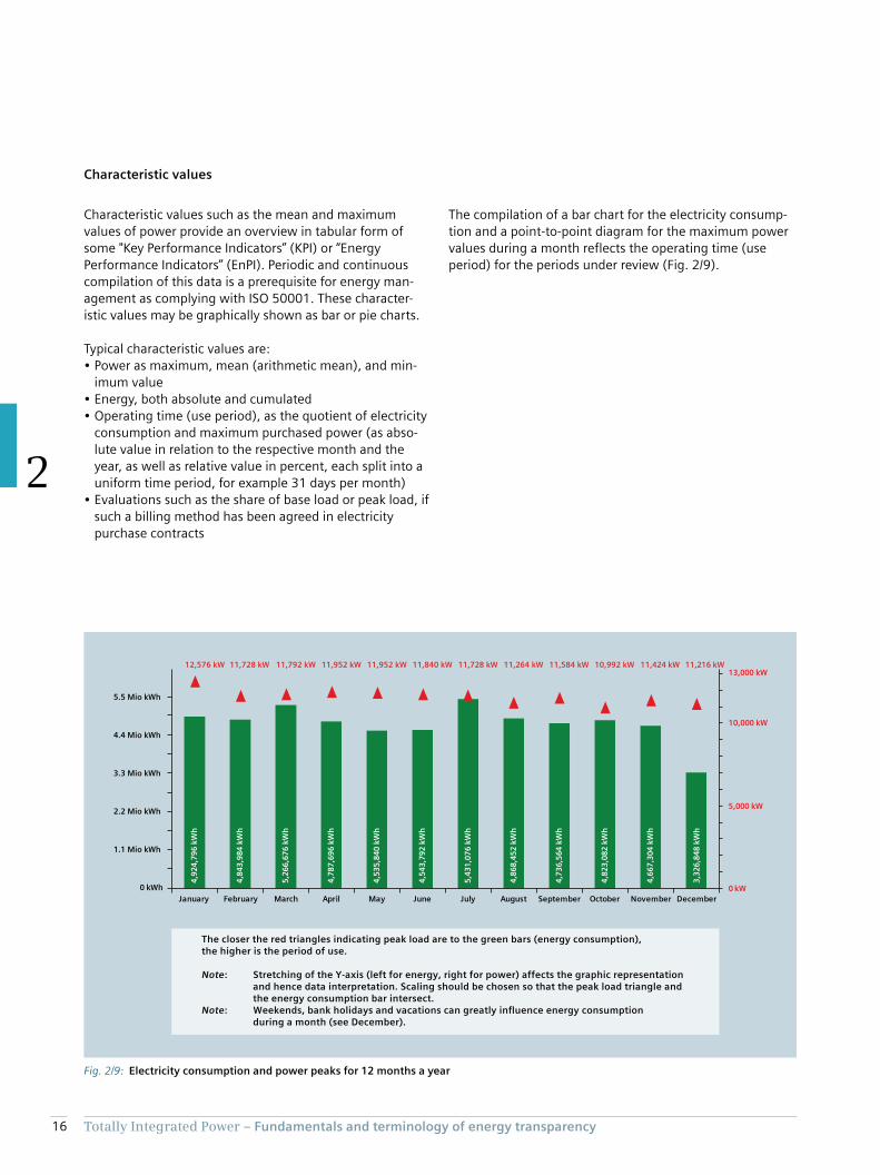
Characteristic values
Characteristic values such as the mean and maximum
values of power provide an overview in tabular form of
some "Key Performance Indicators” (KPI) or “Energy
Performance Indicators” (EnPI). Periodic and continuous
compilation of this data is a prerequisite for energy man-
agement as complying with ISO 50001. These character-
istic values may be graphically shown as bar or pie charts.
Typical characteristic values are:
• Power as maximum, mean (arithmetic mean), and min-
imum value
• Energy, both absolute and cumulated
• Operating time (use period), as the quotient of electricity
consumption and maximum purchased power (as abso-
lute value in relation to the respective month and the
year, as well as relative value in percent, each split into a
uniform time period, for example 31 days per month)
• Evaluations such as the share of base load or peak load, if
such a billing method has been agreed in electricity
purchase contracts
The compilation of a bar chart for the electricity consump-
tion and a point-to-point diagram for the maximum power
values during a month reflects the operating time (use
period) for the periods under review (Fig. 2/9).
Fig. 2/9: Electricity consumption and power peaks for 12 months a year
12,576 kW 11,728 kW 11,792 kW 11,952 kW 11,952 kW 11,840 kW 11,728 kW 11,264 kW 11,584 kW 10,992 kW 11,424 kW 11,216 kW
4,9
24
,79
6 k
Wh
4,8
43
,98
4 k
Wh
5,2
66
,67
6 k
Wh
4,7
87
,69
6 k
Wh
4,5
35
,84
0 k
Wh
4,5
43
,79
2 k
Wh
5,4
31
,07
6 k
Wh
4,8
68
,45
2 k
Wh
4,7
36
,56
4 k
Wh
4,8
23
,08
2 k
Wh
4,6
67
,30
4 k
Wh
3,3
26
,84
8 k
Wh
January February March April May June July August September October November December
0 kW
13,000 kW
1.1 Mio kWh
5.5 Mio kWh
0 kWh
4.4 Mio kWh
3.3 Mio kWh
2.2 Mio kWh
10,000 kW
5,000 kW
The closer the red triangles indicating peak load are to the green bars (energy consumption), the higher is the period of use.
Note: Stretching of the Y-axis (left for energy, right for power) affects the graphic representation and hence data interpretation. Scaling should be chosen so that the peak load triangle and the energy consumption bar intersect.Note: Weekends, bank holidays and vacations can greatly influence energy consumption during a month (see December).
17Totally Integrated Power – Fundamentals and terminology of energy transparency
2
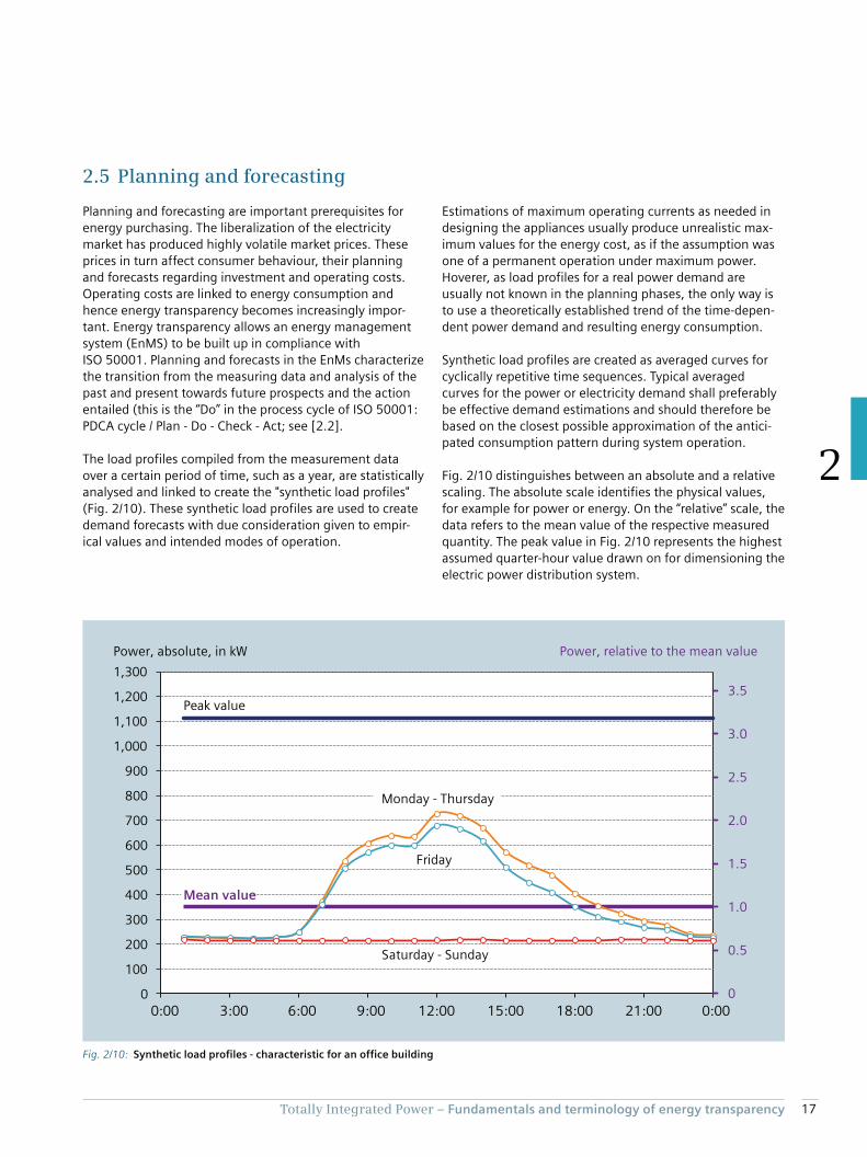
2.5 Planning and forecasting
Planning and forecasting are important prerequisites for
energy purchasing. The liberalization of the electricity
market has produced highly volatile market prices. These
prices in turn affect consumer behaviour, their planning
and forecasts regarding investment and operating costs.
Operating costs are linked to energy consumption and
hence energy transparency becomes increasingly impor-
tant. Energy transparency allows an energy management
system (EnMS) to be built up in compliance with
ISO 50001. Planning and forecasts in the EnMs characterize
the transition from the measuring data and analysis of the
past and present towards future prospects and the action
entailed (this is the “Do” in the process cycle of ISO 50001:
PDCA cycle / Plan - Do - Check - Act; see [2.2].
The load profiles compiled from the measurement data
over a certain period of time, such as a year, are statistically
analysed and linked to create the "synthetic load profiles"
(Fig. 2/10). These synthetic load profiles are used to create
demand forecasts with due consideration given to empir-
ical values and intended modes of operation.
Estimations of maximum operating currents as needed in
designing the appliances usually produce unrealistic max-
imum values for the energy cost, as if the assumption was
one of a permanent operation under maximum power.
Hoverer, as load profiles for a real power demand are
usually not known in the planning phases, the only way is
to use a theoretically established trend of the time-depen-
dent power demand and resulting energy consumption.
Synthetic load profiles are created as averaged curves for
cyclically repetitive time sequences. Typical averaged
curves for the power or electricity demand shall preferably
be effective demand estimations and should therefore be
based on the closest possible approximation of the antici-
pated consumption pattern during system operation.
Fig. 2/10 distinguishes between an absolute and a relative
scaling. The absolute scale identifies the physical values,
for example for power or energy. On the “relative” scale, the
data refers to the mean value of the respective measured
quantity. The peak value in Fig. 2/10 represents the highest
assumed quarter-hour value drawn on for dimensioning the
electric power distribution system.
Fig. 2/10: Synthetic load profiles - characteristic for an office building
0:00 0:0021:0018:0015:0012:009:006:003:000
100
1,000
1,100
1,300
Power, absolute, in kW
Peak value
Mean value
Friday
Monday - Thursday
Saturday - Sunday
1,200
900
800
700
600
500
400
300
200
0
0.5
3.5
3.0
2.5
2.0
1.5
1.0
Power, relative to the mean value
18 Totally Integrated Power – Fundamentals and terminology of energy transparency
2
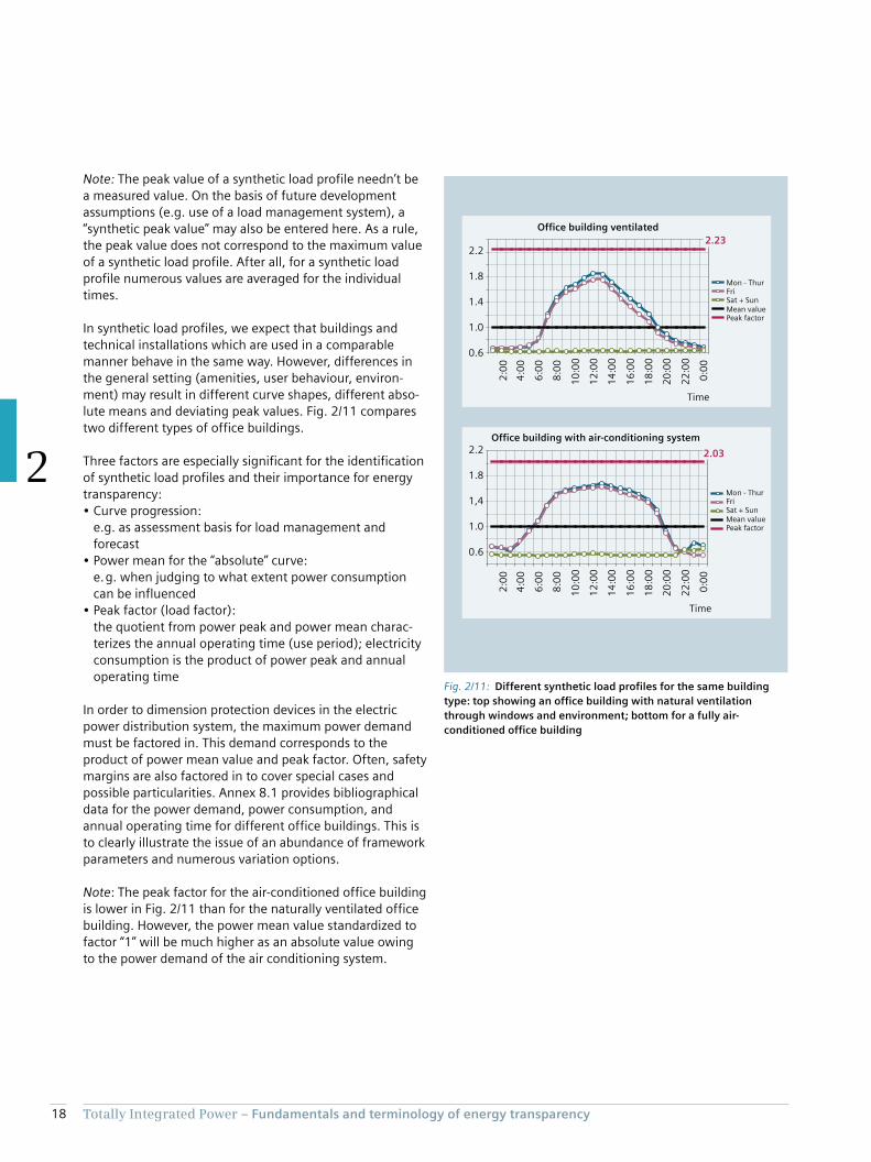
Note: The peak value of a synthetic load profile needn’t be
a measured value. On the basis of future development
assumptions (e.g. use of a load management system), a
“synthetic peak value” may also be entered here. As a rule,
the peak value does not correspond to the maximum value
of a synthetic load profile. After all, for a synthetic load
profile numerous values are averaged for the individual
times.
In synthetic load profiles, we expect that buildings and
technical installations which are used in a comparable
manner behave in the same way. However, differences in
the general setting (amenities, user behaviour, environ-
ment) may result in different curve shapes, different abso-
lute means and deviating peak values. Fig. 2/11 compares
two different types of office buildings.
Three factors are especially significant for the identification
of synthetic load profiles and their importance for energy
transparency:
• Curve progression:
e.g. as assessment basis for load management and
forecast
• Power mean for the “absolute” curve:
e. g. when judging to what extent power consumption
can be influenced
• Peak factor (load factor):
the quotient from power peak and power mean charac-
terizes the annual operating time (use period); electricity
consumption is the product of power peak and annual
operating time
In order to dimension protection devices in the electric
power distribution system, the maximum power demand
must be factored in. This demand corresponds to the
product of power mean value and peak factor. Often, safety
margins are also factored in to cover special cases and
possible particularities. Annex 8.1 provides bibliographical
data for the power demand, power consumption, and
annual operating time for different office buildings. This is
to clearly illustrate the issue of an abundance of framework
parameters and numerous variation options.
Note: The peak factor for the air-conditioned office building
is lower in Fig. 2/11 than for the naturally ventilated office
building. However, the power mean value standardized to
factor “1” will be much higher as an absolute value owing
to the power demand of the air conditioning system.
Fig. 2/11: Different synthetic load profiles for the same building
type: top showing an office building with natural ventilation
through windows and environment; bottom for a fully air-
conditioned office building
2:0
0
4:0
0
6:0
0
8:0
0
10
:00
12
:00
14
:00
16
:00
18
:00
20
:00
22
:00
0:0
0
2:0
0
4:0
0
6:0
0
8:0
0
10
:00
12
:00
14
:00
16
:00
18
:00
20
:00
22
:00
0:0
0
Office building ventilated
2.23
Time
Mon - ThurFriSat + SunMean valuePeak factor
Office building with air-conditioning system
Time
2.03
Mon - ThurFriSat + SunMean valuePeak factor
2.2
1.8
1.4
1.0
0.6
2.2
1.8
1,4
1.0
0.6
Chapter 3Measured value acquisition in the distribution grid and its importance in the electricity market
3.1 Measured quantities and characteristic parameters in the customer’s power system 22
3.2 Deriving synthetic load curves 24
3.3 Forecasts and the electricity market 25
20 Totally Integrated Power – Measured value acquisition in the distribution grid and its importance in the electricity market
3
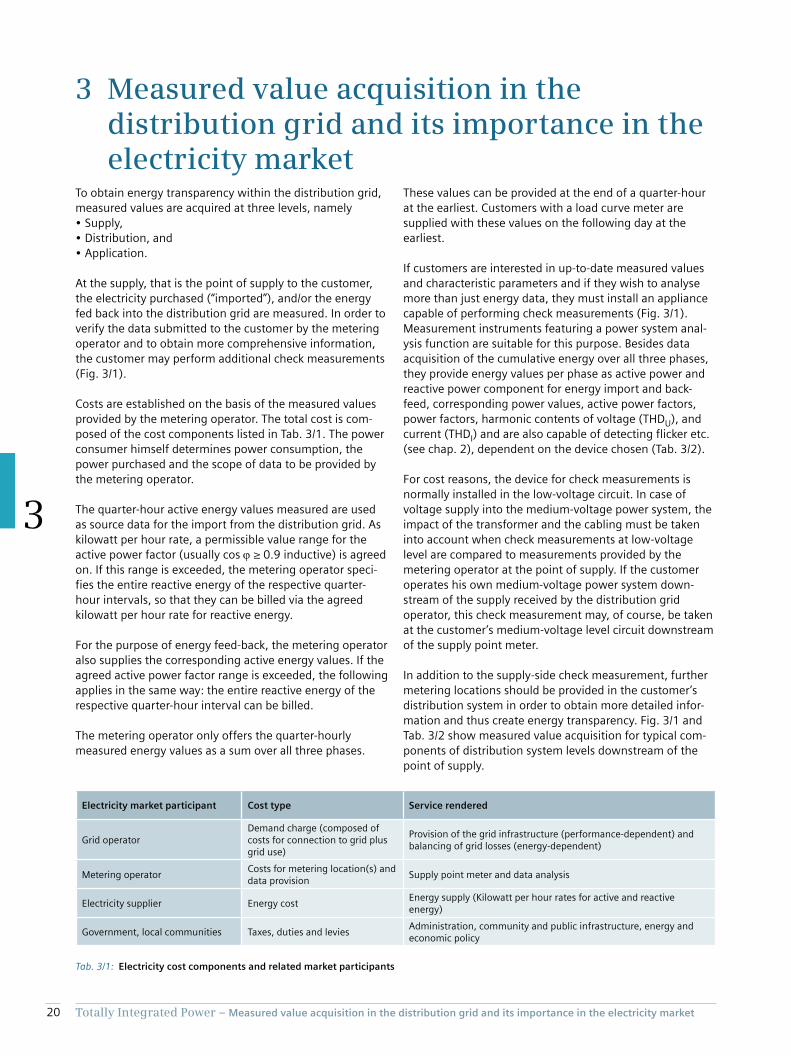
3 Measured value acquisition in the distribution grid and its importance in the electricity market
To obtain energy transparency within the distribution grid,
measured values are acquired at three levels, namely
• Supply,
• Distribution, and
• Application.
At the supply, that is the point of supply to the customer,
the electricity purchased (“imported”), and/or the energy
fed back into the distribution grid are measured. In order to
verify the data submitted to the customer by the metering
operator and to obtain more comprehensive information,
the customer may perform additional check measurements
(Fig. 3/1).
Costs are established on the basis of the measured values
provided by the metering operator. The total cost is com-
posed of the cost components listed in Tab. 3/1. The power
consumer himself determines power consumption, the
power purchased and the scope of data to be provided by
the metering operator.
The quarter-hour active energy values measured are used
as source data for the import from the distribution grid. As
kilowatt per hour rate, a permissible value range for the
active power factor (usually cos ≥ 0.9 inductive) is agreed
on. If this range is exceeded, the metering operator speci-
fies the entire reactive energy of the respective quarter-
hour intervals, so that they can be billed via the agreed
kilowatt per hour rate for reactive energy.
For the purpose of energy feed-back, the metering operator
also supplies the corresponding active energy values. If the
agreed active power factor range is exceeded, the following
applies in the same way: the entire reactive energy of the
respective quarter-hour interval can be billed.
The metering operator only offers the quarter-hourly
measured energy values as a sum over all three phases.
Tab. 3/1: Electricity cost components and related market participants
Electricity market participant Cost type Service rendered
Grid operatorDemand charge (composed of costs for connection to grid plus grid use)
Provision of the grid infrastructure (performance-dependent) and balancing of grid losses (energy-dependent)
Metering operatorCosts for metering location(s) and data provision
Supply point meter and data analysis
Electricity supplier Energy costEnergy supply (Kilowatt per hour rates for active and reactive energy)
Government, local communities Taxes, duties and leviesAdministration, community and public infrastructure, energy and economic policy
These values can be provided at the end of a quarter-hour
at the earliest. Customers with a load curve meter are
supplied with these values on the following day at the
earliest.
If customers are interested in up-to-date measured values
and characteristic parameters and if they wish to analyse
more than just energy data, they must install an appliance
capable of performing check measurements (Fig. 3/1).
Measurement instruments featuring a power system anal-
ysis function are suitable for this purpose. Besides data
acquisition of the cumulative energy over all three phases,
they provide energy values per phase as active power and
reactive power component for energy import and back-
feed, corresponding power values, active power factors,
power factors, harmonic contents of voltage (THDU), and
current (THDI) and are also capable of detecting flicker etc.
(see chap. 2), dependent on the device chosen (Tab. 3/2).
For cost reasons, the device for check measurements is
normally installed in the low-voltage circuit. In case of
voltage supply into the medium-voltage power system, the
impact of the transformer and the cabling must be taken
into account when check measurements at low-voltage
level are compared to measurements provided by the
metering operator at the point of supply. If the customer
operates his own medium-voltage power system down-
stream of the supply received by the distribution grid
operator, this check measurement may, of course, be taken
at the customer’s medium-voltage level circuit downstream
of the supply point meter.
In addition to the supply-side check measurement, further
metering locations should be provided in the customer’s
distribution system in order to obtain more detailed infor-
mation and thus create energy transparency. Fig. 3/1 and
Tab. 3/2 show measured value acquisition for typical com-
ponents of distribution system levels downstream of the
point of supply.
21Totally Integrated Power – Measured value acquisition in the distribution grid and its importance in the electricity market
3
Tab. 3/2: Measured values and characteristic parameters at various locations in the customer’s power system
1) 1) 1)
1)
T
Z
G
E
V1
V2
V3
V4
K
WQ WQW W S PSL1,
SL2,
SL3
PL1,
PL2,
PL3
Q QL1,
QL2,
QL3
UL1-L2,
UL2-L3,
UL3-L1
UL1-N,
UL2-N,
UL3-N
IL1,
IL2,
IL3
IN cos L1,
cos L2,
cos L3
cos L1,
L2,
L3
THDIL1,
THDIL2,
THDIL3
THDUL1-L2,
THDUL2-L3,
THDUL3-L1
kWh VkvarkvarkWkWkVAkVAkvarhkvarhkWh %A %V A
Act
ive
en
erg
yIm
po
rt
Act
ive
en
erg
yB
ack
fee
d
Re
act
ive
en
erg
yIm
po
rt
Re
act
ive
en
erg
yB
ack
fee
d
Ap
pa
ren
t e
ne
rgy
sum
Ap
pa
ren
t p
ow
er
pe
r p
ha
se
Ap
pa
ren
t p
ow
er
sum
Act
ive
po
we
rp
er
ph
ase
Re
act
ive
po
we
rsu
m
Re
act
ive
po
we
rp
er
ph
ase
Vo
lta
ge
ph
ase
-ph
ase
Vo
lta
ge
ph
ase
-ne
utr
al
Ph
ase
cu
rre
nt
Ne
utr
al
curr
en
t
Act
ive
po
we
r fa
cto
rsu
m
Act
ive
po
we
r fa
cto
rp
er
ph
ase
Po
we
r fa
cto
rs H
arm
on
ics
pe
rp
ha
se c
urr
en
t
Ha
rmo
nic
s p
er
ph
ase
-to
-ph
ase
vo
lta
ge
Measured values of metering operator Check measurement Transformer feeder Generator feeder Energy distribution Load, symmetric linear Load, asymmetric linear Load, asymmetric non-linear Load – cost centre allocation, energy billing
1) optional measurement
Measured quantities /characteristic parameters
Formula symbols
Units
Fig. 3/1: Measured values and characteristic parameters at the various distribution levels
Z
G
M P P P
T
KG
V1 V2 V3 V4
E
T
K
Z
G
E
V1
V2
V3
V4
Check measurement
Transformer feeder
Supply point meter
Supply
Generator feeder
Power distribution
Load - 3-phase, linear symmetrical, e.g. motor
Load - linear and asymmetrical, e.g. floor distribution board
Load - non-linear and asymmetrical, e.g. electronic switching device
Load - cost centre allocation, energy billing
Distribution
Loads
22 Totally Integrated Power – Measured value acquisition in the distribution grid and its importance in the electricity market
3
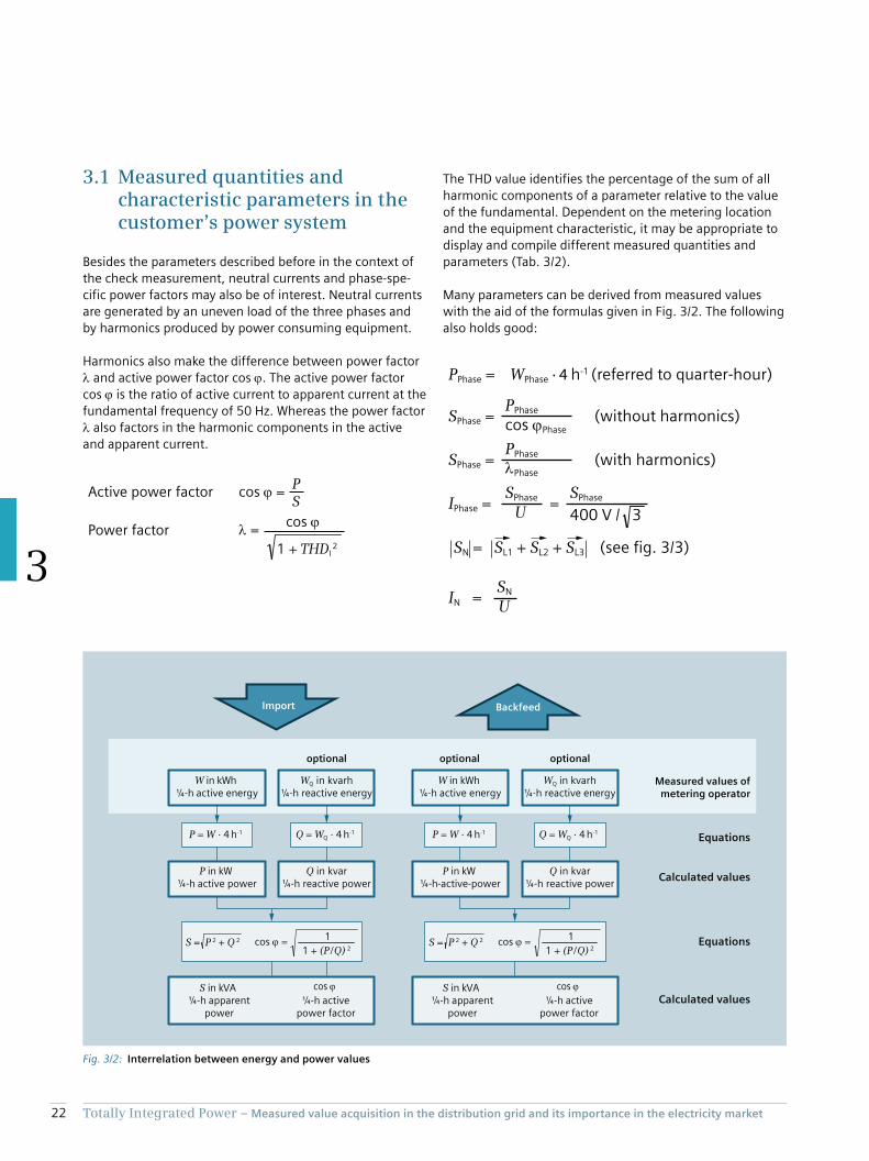
The THD value identifies the percentage of the sum of all
harmonic components of a parameter relative to the value
of the fundamental. Dependent on the metering location
and the equipment characteristic, it may be appropriate to
display and compile different measured quantities and
parameters (Tab. 3/2).
Many parameters can be derived from measured values
with the aid of the formulas given in Fig. 3/2. The following
also holds good:
cos =P
S
=
Active power factor
Power factor
cos
1 + THDI 2
PPhase = WPhase · 4 h-1 (referred to quarter-hour)
cos Phase
Phase
U 400 V / 3
U
SPhase = (without harmonics)PPhase
SPhase = (with harmonics)PPhase
IPhase = =SPhase SPhase
SN = SL1 + SL2 + SL3 (see fig. 3/3)
IN =SN
3.1 Measured quantities and characteristic parameters in the customer’s power system
Besides the parameters described before in the context of
the check measurement, neutral currents and phase-spe-
cific power factors may also be of interest. Neutral currents
are generated by an uneven load of the three phases and
by harmonics produced by power consuming equipment.
Harmonics also make the difference between power factor
and active power factor cos . The active power factor
cos is the ratio of active current to apparent current at the
fundamental frequency of 50 Hz. Whereas the power factor
also factors in the harmonic components in the active
and apparent current.
Fig. 3/2: Interrelation between energy and power values
W in kWh ¼-h active energy
WQ in kvarh¼-h reactive energy
optional
Import
optional
Backfeed
optional
Measured values ofmetering operator
Calculated values
Calculated values
P in kW ¼-h active power
Q in kvar¼-h reactive power
S in kVA ¼-h apparent
power
cos
¼-h activepower factor
S in kVA ¼-h apparent
power
cos
¼-h activepower factor
Equations
Equations
W in kWh ¼-h active energy
WQ in kvarh¼-h reactive energy
P in kW ¼-h-active-power
Q in kvar¼-h reactive power
S = P 2 + Q 2
P = W · 4 h-1 Q = WQ · 4 h-1
cos =1
1 + (P / Q) 2
P = W · 4 h-1 Q = WQ · 4 h-1
S = P 2 + Q 2 cos =1
1 + (P / Q) 2
23Totally Integrated Power – Measured value acquisition in the distribution grid and its importance in the electricity market
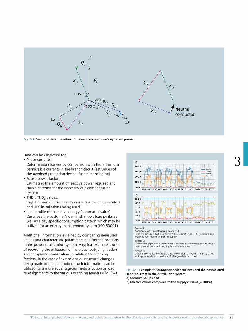
3Data can be employed for:
• Phase currents:
Determining reserves by comparison with the maximum
permissible currents in the branch circuit (set values of
the overload protection device, fuse dimensioning)
• Active power factor:
Estimating the amount of reactive power required and
thus a criterion for the necessity of a compensation
system
• THDI , THDU values:
High harmonic currents may cause trouble on generators
and UPS installations being used
• Load profile of the active energy (summated value)
Describes the customer’s demand, shows load peaks as
well as a day-specific consumption pattern which may be
utilized for an energy management system (ISO 50001)
Additional information is gained by comparing measured
values and characteristic parameters at different locations
in the power distribution system. A typical example is one
of recording the utilization of individual outgoing feeders
and comparing these values in relation to incoming
feeders. In the case of extensions or structural changes
being made in the distribution, such information can be
utilized for a more advantageous re-distribution or load
re-assignments to the various outgoing feeders (Fig. 3/4).
Fig. 3/3: Vectorial determination of the neutral conductor’s apparent power
L1
L2L3
PL1
cos L1
QL2
QL1
SL3
SL2
SL1
PL3
PL2
QL3
cos L3
cos L2
SL3
SL2
SL1
Neutralconductor
Fig. 3/4: Example for outgoing feeder currents and their associated
supply current in the distribution system;
a) absolute values and
b) relative values compared to the supply current (= 100 %)
0 A
300 A
100 A
200 A
a)
400 A
0 %
80 %
40 %
20 %
60 %
100 %
b)
Supply
Feeder 3
Feeder 2
Feeder 1
Feeder 3:Apparently, only small loads are connected;Relations between daytime and night-time operation as well as weekend and weekday operation correspond to supply
Feeder 2:Demand for night-time operation and weekends nearly corresponds to the full power quantity supplied; possibly for safety equipment
Feeder 1:Daytime use; noticeable are the three power dips at around 10 a. m., 2 p. m.,and 6 p. m. (early shift break – shift change – late shift break)
Mon 19.05. Tue 20.05. Wed 21.05. Thur 22.05. Fri 23.05. Sat 24.05. Sun 25.05.
Mon 19.05. Tue 20.05. Wed 21.05. Thur 22.05. Fri 23.05. Sat 24.05. Sun 25.05.
24 Totally Integrated Power – Measured value acquisition in the distribution grid and its importance in the electricity market
3
3.2 Derivation from synthetic load curves
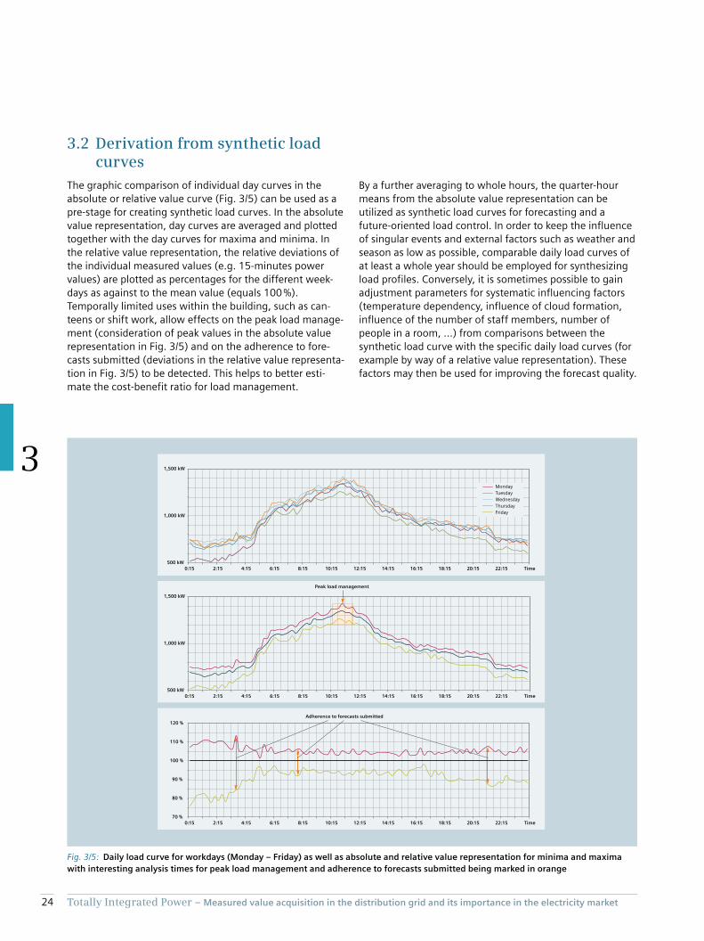
The graphic comparison of individual day curves in the
absolute or relative value curve (Fig. 3/5) can be used as a
pre-stage for creating synthetic load curves. In the absolute
value representation, day curves are averaged and plotted
together with the day curves for maxima and minima. In
the relative value representation, the relative deviations of
the individual measured values (e.g. 15-minutes power
values) are plotted as percentages for the different week-
days as against to the mean value (equals 100 %).
Temporally limited uses within the building, such as can-
teens or shift work, allow effects on the peak load manage-
ment (consideration of peak values in the absolute value
representation in Fig. 3/5) and on the adherence to fore-
casts submitted (deviations in the relative value representa-
tion in Fig. 3/5) to be detected. This helps to better esti-
mate the cost-benefit ratio for load management.
By a further averaging to whole hours, the quarter-hour
means from the absolute value representation can be
utilized as synthetic load curves for forecasting and a
future-oriented load control. In order to keep the influence
of singular events and external factors such as weather and
season as low as possible, comparable daily load curves of
at least a whole year should be employed for synthesizing
load profiles. Conversely, it is sometimes possible to gain
adjustment parameters for systematic influencing factors
(temperature dependency, influence of cloud formation,
influence of the number of staff members, number of
people in a room, ...) from comparisons between the
synthetic load curve with the specific daily load curves (for
example by way of a relative value representation). These
factors may then be used for improving the forecast quality.
Fig. 3/5: Daily load curve for workdays (Monday – Friday) as well as absolute and relative value representation for minima and maxima
with interesting analysis times for peak load management and adherence to forecasts submitted being marked in orange
500 kW
500 kW
70 %
90 %
80 %
120 %
110 %
100 %
1,500 kW
1,000 kW
1,500 kW
1,000 kW
Monday
Tuesday
Wednesday
Thursday
Friday
0:15 2:15 4:15 6:15 8:15 10:15 12:15 14:15 16:15 18:15 20:15 22:15 Time
0:15 2:15 4:15 6:15 8:15 10:15 12:15 14:15 16:15 18:15 20:15 22:15 Time
Peak load management
0:15 2:15 4:15 6:15 8:15 10:15 12:15 14:15 16:15 18:15 20:15 22:15 Time
Adherence to forecasts submitted
25Totally Integrated Power – Measured value acquisition in the distribution grid and its importance in the electricity market
3
3.3 Forecasts and the electricity market
The importance of consumption forecasts is going to
increase. Whereas smart meters have previously been
installed upwards of an annual energy consumption above
100,000 kWh/a, such meters will in future be mounted
upwards of an electricity consumption of more than
60,000 kWh/a. With the data the electricity supplier
receives from the metering operator, he is able to assess
consumer behaviour. Since the electricity supplier must
back his electricity purchase by forecasts, he will be
charged for additional costs in case of deviations from the
forecast. He will forward these additional costs - based on
the data received - to his customers who do not adhere to
their forecasts.
For periods of more than a week, long-term forecasts are
created. Correspondingly, electricity suppliers cover their
demand by directly buying from power station operators
and/or from the electricity exchange. Energy forecasts for
the following week (usually on a Thursday covering the
seven days of the following week) result in fairly accurate
load profiles. Weather forecasts for calculating wind power
and solar energy also go into these forecasts. These
weather forecasts are provided by specialized companies
with a prediction accuracy of more than 90 %.
Deviations as occurring during operations from the long-
term and the weekly forecast are offset as much as possible
by purchase and sale through the electricity exchange. In
order to take account of short-term changes, the adjust-
ment between weekly and daily forecast is performed every
day. Here too, differences are offset through the exchange
(“day-ahead trade”). The smallest unit of a target-actual
adjustment is a quarter-hour within the subsequent hour.
These difference quantities are traded in the “intraday
trade” at the electricity exchange (see chap. 1 and [3.1]).
For the consumer it is a matter of adapting every quarter-
hour demand as closely to the forecast submitted as pos-
sible (see Fig. 1/3). Extra consumption must often be dearly
bought, since the electricity supplier must order this addi-
tional quantity through a balancing reserve. Conversely,
less consumption may not result in a cost reduction for the
consumer.
Aggregation into an overall forecast
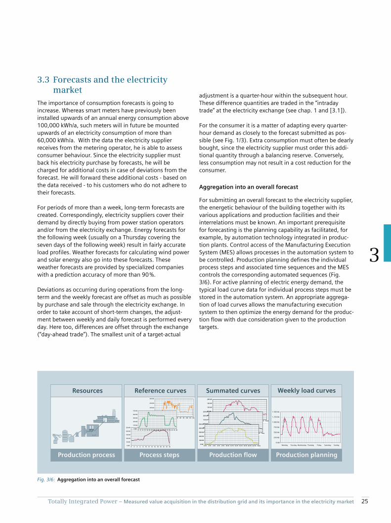
For submitting an overall forecast to the electricity supplier,
the energetic behaviour of the building together with its
various applications and production facilities and their
interrelations must be known. An important prerequisite
for forecasting is the planning capability as facilitated, for
example, by automation technology integrated in produc-
tion plants. Control access of the Manufacturing Execution
System (MES) allows processes in the automation system to
be controlled. Production planning defines the individual
process steps and associated time sequences and the MES
controls the corresponding automated sequences (Fig.
3/6). For active planning of electric energy demand, the
typical load curve data for individual process steps must be
stored in the automation system. An appropriate aggrega-
tion of load curves allows the manufacturing execution
system to then optimize the energy demand for the produc-
tion flow with due consideration given to the production
targets.
Fig. 3/6: Aggregation into an overall forecast
300 kW
0 10 20 30 40 50 60 12070 80 10090 110
150 kW
600 kW
450 kW
0 kW
200 kW
80 kW
0:15 2:15 4:15 6:15 8:15 10:15 12:15 14:15 16:15 18:15 20:15 22:15
Uhrzeit
40 kW
160 kW
120 kW
0 kW
250 kW
100 kW
0:15 2:15 4:15 6:15 8:15 10:15 12:15 14:15 16:15 18:15 20:15 22:15
Uhrzeit
50 kW
200 kW
150 kW
0 kW
500 kW
200 kW
0:15 2:15 4:15 6:15 8:15 10:15 12:15 14:15 16:15 18:15 20:15 22:15
Uhrzeit
100 kW
400 kW
300 kW
0 kW
250 kW
100 kW
0 2 4 6 8 12 16 20 2410 14 18 22 26
50 kW
200 kW
150 kW
0 kW
750 kW
300 kW
0 4 8 12 16 20 24 28 32 36 6840 44 48 52 56 60 64
150 kW
600 kW
450 kW
0 kW
Monday Tuesday Wednesday Thursday Friday Saturday Sunday
0 kW
1.250 kW
1.000 kW
750 kW
500 kW
250 kW
1.500 kW
Production process Process steps Production flow Production planning
Resources Reference curves Summated curves Weekly load curves
Time
Time
Time

26 Totally Integrated Power – Measured value acquisition in the distribution grid and its importance in the electricity market
3
Controlling and switching
To level out deviations from submitted forecasts, loads can
be connected into or disconnected from supply and can be
curbed or increased by means of a load management
system (Fig. 3/7). Innumerable switching and control
strategies dependent on the respective applications and
targets can often be applied.
A priority list containing switching and control data about
the various loads is a good aid for creating and imple-
menting suitable strategies. This list includes data of when
and how which load, power generator, or energy storage
device and which switch, regulator, or control device can
be applied (keyword: “characteristics”). For the controllable
loads this also means defining the control range and their
response time. Switching devices for load management
must be chosen according to product-specific operating
cycles and the profiles to be expected. Load management
flexibility is characterized by an overlay and link-up of
response options which in keeping with the given condi-
tions are feasible at certain points in time and under the
usage targets set.
Fig. 3/7: Consumption adjustment using strategical load management
M M
Release
Block
Release
block
Feedback
Forced ON
ON OFF
Feedback
Forced ON
Actual values
Target values
ON OFF
Priority listof manipulable loads and power generators
Load 1
Load 2
Load 3
Load n-1
Load n
Connect Disconnect
Load control• Controlling • Adjusting
Characteristicsof manipulable loads and power generators
Flexibilityis gained from the characteristics of loads and power generators as well as ambient and operating conditions
• Type Power generator Load Energy storage system
• Type Switchable Adjustable
• Constraints Maximum runtime Minimum runtime Maximum standstill time
• Additional data Base load (standby) Manipulable power Connect/disconnect power
• Signals Released/blocked Feedback Forced ON Power measurements
0
20
200
Power in kW
Power: Demand Connectable Disconnectable
180
160
140
120
100
80
60
40
Time
0:00 8:007:006:005:004:003:002:001:00
Controllable / adjustable range

27Totally Integrated Power – Measured value acquisition in the distribution grid and its importance in the electricity market
3
The prosumer
When the customer combines his own power generation,
for example from renewable power sources and combined
heat and power generating plants with his own consump-
tion and power supply from the supply grid (Fig. 3/8),
planning should make provisions to integrate and link as
many framework parameters for load management as
possible:
• Synthetic load curves for the customer’s own demand
• Power output forecast for a photovoltaic system linked to
the weather data for solar radiation
• Power output linked to the heat demand over time for a
heat-controlled CHP plant
In addition, ongoing changes in production planning and in
process steps ranging up to start and stop conditions for
machinery and production lines must be taken into
account. Similarly, staff deployment options and further
operational and servicing conditions can be employed to
draw up a reliable consumption schedule. Energy transpar-
ency and the derivable relations and forecasts are impor-
tant for a “prosumer” (who is simultaneously a producer
and consumer of energy) to optimize his forecasting effec-
tiveness or to utilize the existing flexibility to his benefit.
Fig. 3/8: Combination of power consumption and generation
Date
Power in kW
150
125
100
75
50
25
0
Date
Power in kW
150
100
50
0
-50
-150
-100
Date
Power in kW
300
250
200
150
100
0
50
Date
Power in kW
120
100
80
60
40
20
0
22.09. 27.09.26.09.25.09.24.09.23.09. 28.09. 22.09. 27.09.26.09.25.09.24.09.23.09. 28.09.
22.09. 27.09.26.09.25.09.24.09.23.09. 28.09.
22.09. 27.09.26.09.25.09.24.09.23.09. 28.09.
28 Totally Integrated Power – Measured value acquisition in the distribution grid and its importance in the electricity market
3
Electricity market
In Germany, the increase of power generated on the elec-
tricity customer’s own premises or plant goes hand in hand
with the restructuring of the electricity market (“Electricity
Market 2.0” see draft for an Electricity Market Act [3.2]).
A possible consequence of this is an increasing demand for
power stations enabling load controlling and peak load
power stations as well as a rising demand for flexibility in
consumption behaviour or for storage possibilities. At the
same time, the expectation is for electricity trading to be
performed efficiently through various sub-markets
(Electricity Exchange as well as extra-exchange “over the
counter”), see White Paper [3.3]. This means employing
prices on the electricity and power market to control elec-
tricity generation and consumption.
Incentives for balancing group loyalty are being enhanced.
Any deviation from it should be settled according to the
“user pays” principle through the expensive balancing
energy system with the balancing group manager. Access
to the secondary balancing power market will be facilitated
for service providers in the load management sector [3.2].
In particular, remote-controlled power reductions or discon-
nections of power generating sets may be part of the
action plan of grid operators (negative balancing power in
Fig. 3/9). In Germany, the Renewable Energies Act (EEG
2017) [3.2] and [3.4] and the Combined Heat and Power
Act (KWK-G) [3.5] govern the requirements of power
control and power metering by the grid operator
conditional upon the power supplied (>100 kW) by renew-
able power generation and combined heat and power
plants.
According to EEG and KWK-G there is an obligation on the
part of the grid operator to connect renewable power
generation plants and highly efficient combined heat and
power plants to the grid. This is to enable trading of the
electricity fed in. The different acceptance obligations and
remunerations including premium or surcharge payments
can be found in the current publications of the two acts.
Current prices for electricity supplied from CHP plants can
be found on the web pages of the Leipzig EEX, referred to
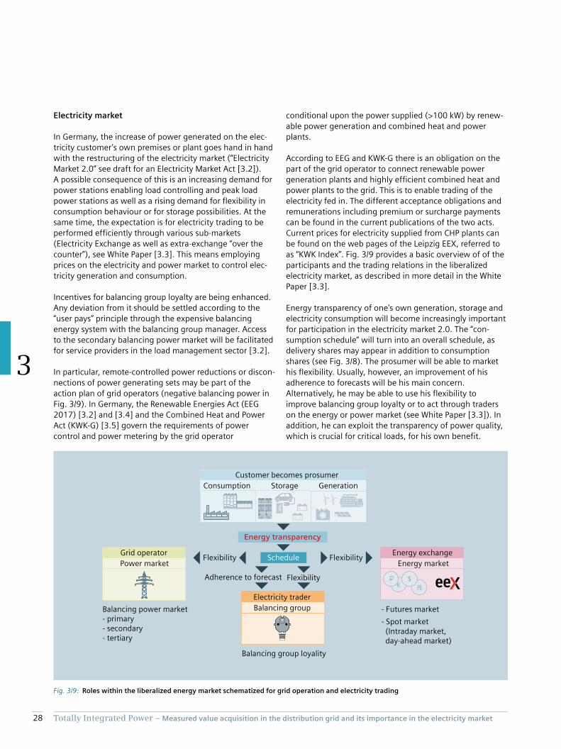
as “KWK Index”. Fig. 3/9 provides a basic overview of of the
participants and the trading relations in the liberalized
electricity market, as described in more detail in the White
Paper [3.3].
Energy transparency of one's own generation, storage and
electricity consumption will become increasingly important
for participation in the electricity market 2.0. The “con-
sumption schedule” will turn into an overall schedule, as
delivery shares may appear in addition to consumption
shares (see Fig. 3/8). The prosumer will be able to market
his flexibility. Usually, however, an improvement of his
adherence to forecasts will be his main concern.
Alternatively, he may be able to use his flexibility to
improve balancing group loyalty or to act through traders
on the energy or power market (see White Paper [3.3]). In
addition, he can exploit the transparency of power quality,
which is crucial for critical loads, for his own benefit.
Fig. 3/9: Roles within the liberalized energy market schematized for grid operation and electricity trading
€ 元$

Chapter 4Operational performance and efficiency in electric power distribution
4.1. Transformer performance 30
4.2. Generator performance 32
4.3 Motor and assembly control and adjustment 33
4.4 Distributed generation of electric energy 34
30 Totally Integrated Power – Operational performance and efficiency in electric power distribution
4
4 Operational performance and efficiency in electric power distribution
Energy distribution and consumer energy use generate
losses which are an operating cost factor; this is something
the consumer would prefer to have minimized. Motors and
drives as power consuming equipment contribute substan-
tially to power losses; this is also true for transformers and
generators in the power distribution system.
The most important parameter of an item of equipment is
its efficiency. Efficiency is defined as a quotient of
usable energy and
supplied energy (= output energy + loss energy) as well as
usable power and
supplied power (= usable power + power loss), respectively,
and is usually given as a percentage. The total efficiency
of a whole installation or system is the product of the
individual degrees of efficiency.
total 1 · 2 · 3 · ...
The efficiency can depend on operational and ambient
conditions. However, it is often sufficient just to consider
the degree of loading, since ambient influences such as
operating temperature and heat dissipation are low under
normal operating conditions. Measurements of power and
energy upstream and downstream of an item of equipment
allow the degree of efficiency under given operational
conditions to be established.
4.1 Operating performance of transformers
The effects of harmonics and a parallel operation of trans-
formers will not be considered in this section. In this
respect we would refer the reader to the “Technical Series”
on the web pages of Siemens TIP Consultant Support
(www.siemens.com/tip-cs) and to the support rendered by
our Siemens consultants. For the theoretical determination
of transformer losses, Siemens specifies the no-load and
short-circuit losses of the transformers included in the
product range. Total loss as a function of operational
apparent power is calculated as follows:
The Siemens eco transformers comply with Regulation No.
548/2014 issued by the EU Commission (and thus with the
IEC 60076-20 and VDE 0532-76-20 standard). With an
efficiency of 99 % and more, they meet the highest EEPL4
requirement (EEPL = energy efficiency performance level)
in accordance with IEC 60364-8-1 (VDE 0100-801) in most
cases (only our latest GEAFOL eco transformers with an
apparent power rating below 250 kVA have a 98.5 % to
99 % efficiency).
PV = P0 + (Sload / Sr )2 · Pk
with
PV Transformer power lossP0 No-load loss of transformerPk Short-circuit loss of transformerSload Demand of apparent power during operationSr Rated apparent power of transformer
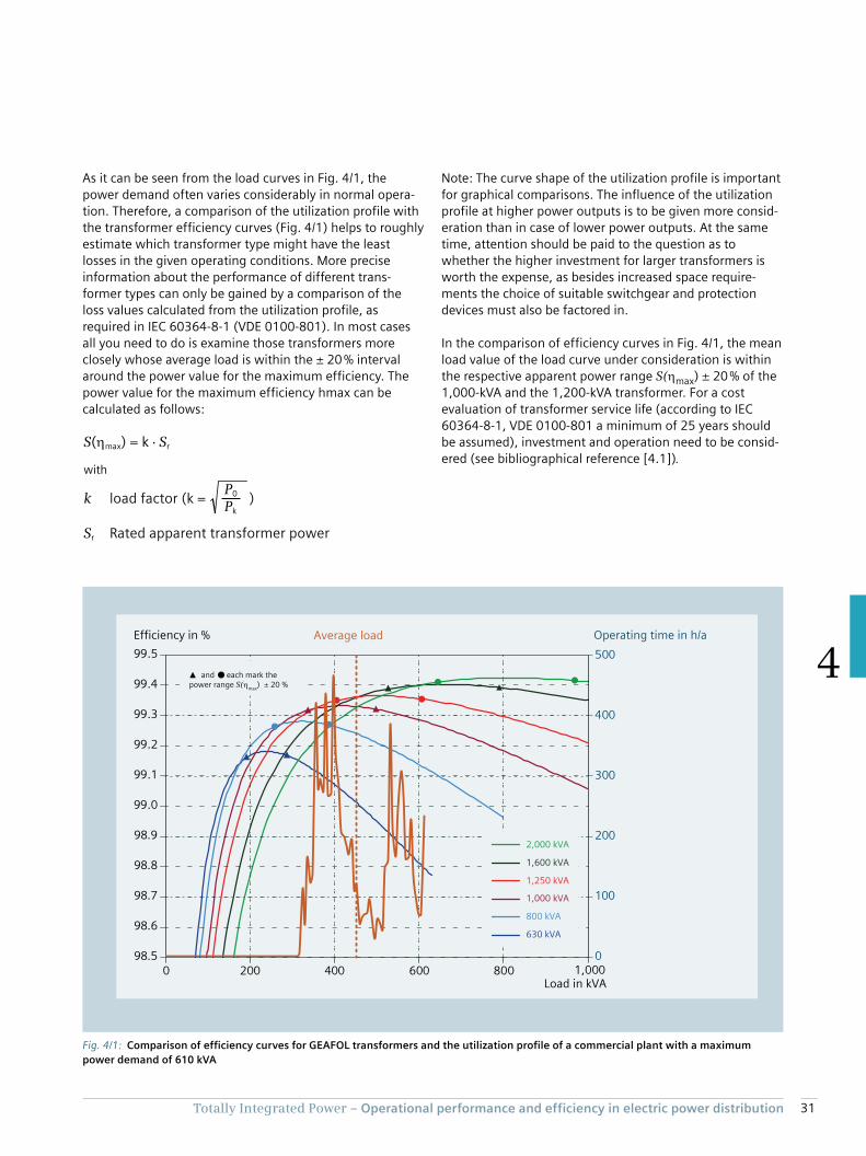
31Totally Integrated Power – Operational performance and efficiency in electric power distribution
4
As it can be seen from the load curves in Fig. 4/1, the
power demand often varies considerably in normal opera-
tion. Therefore, a comparison of the utilization profile with
the transformer efficiency curves (Fig. 4/1) helps to roughly
estimate which transformer type might have the least
losses in the given operating conditions. More precise
information about the performance of different trans-
former types can only be gained by a comparison of the
loss values calculated from the utilization profile, as
required in IEC 60364-8-1 (VDE 0100-801). In most cases
all you need to do is examine those transformers more
closely whose average load is within the ± 20 % interval
around the power value for the maximum efficiency. The
power value for the maximum efficiency hmax can be
calculated as follows:
S max) = k · Sr
with
k load factor (k = )
Sr Rated apparent transformer power
P0
Pk
Note: The curve shape of the utilization profile is important
for graphical comparisons. The influence of the utilization
profile at higher power outputs is to be given more consid-
eration than in case of lower power outputs. At the same
time, attention should be paid to the question as to
whether the higher investment for larger transformers is
worth the expense, as besides increased space require-
ments the choice of suitable switchgear and protection
devices must also be factored in.
In the comparison of efficiency curves in Fig. 4/1, the mean
load value of the load curve under consideration is within
the respective apparent power range S( max) ± 20 % of the
1,000-kVA and the 1,200-kVA transformer. For a cost
evaluation of transformer service life (according to IEC
60364-8-1, VDE 0100-801 a minimum of 25 years should
be assumed), investment and operation need to be consid-
ered (see bibliographical reference [4.1])
Fig. 4/1: Comparison of efficiency curves for GEAFOL transformers and the utilization profile of a commercial plant with a maximum
power demand of 610 kVA
Average load
630 kVA
1,000 kVA
800 kVA
1,250 kVA
2,000 kVA
1,600 kVA
S(
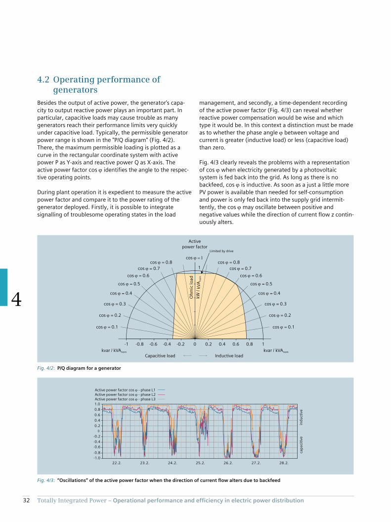
32 Totally Integrated Power – Operational performance and efficiency in electric power distribution
4
4.2 Operating performance of generators
identifies the angle to the respec-
tive operating points.
Fig. 4/2: P/Q diagram for a generator
-1 0 1
1
kvar / kVAnomkvar / kVAnom
Inductive loadCapacitive load
Oh
mic
lo
ad
kW /
kV
An
om
Limited by drive
0.4 0.80.60.2-0.2-0.4-0.6-0.8
Activepower factor
cos
cos = 0.1
cos = 0.8
cos = 0.7
cos = 0.6
cos = 0.5
cos = 0.4
cos = 0.3
cos = 0.2
cos = 0.1
cos = 0.8
cos = 0.7
cos = 0.6
cos = 0.5
cos = 0.4
cos = 0.3
cos = 0.2
Fig. 4/3: “Oscillations” of the active power factor when the direction of current flow alters due to backfeed
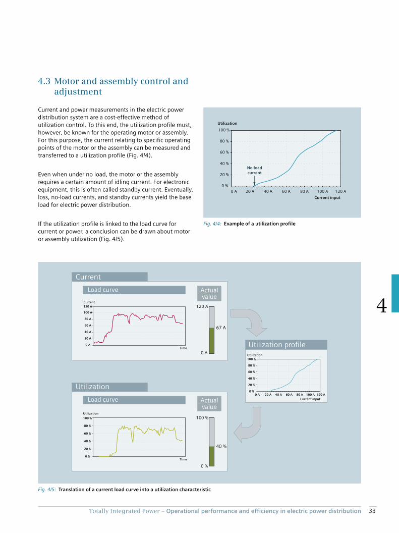
33Totally Integrated Power – Operational performance and efficiency in electric power distribution
4
4.3 Motor and assembly control and adjustment
Current and power measurements in the electric power
distribution system are a cost-effective method of
utilization control. To this end, the utilization profile must,
however, be known for the operating motor or assembly.
For this purpose, the current relating to specific operating
points of the motor or the assembly can be measured and
transferred to a utilization profile (Fig. 4/4).
Even when under no load, the motor or the assembly
requires a certain amount of idling current. For electronic
equipment, this is often called standby current. Eventually,
loss, no-load currents, and standby currents yield the base
load for electric power distribution.
If the utilization profile is linked to the load curve for
current or power, a conclusion can be drawn about motor
or assembly utilization (Fig. 4/5).
Fig. 4/5: Translation of a current load curve into a utilization characteristic
0 %
20 %
40 %
60 %
80 %
100 %
0 A 20 A 40 A 60 A 80 A 100 A 120 A
0 A
20 A
40 A
60 A
80 A
100 A
120 A
0 %
20 %
40 %
60 %
80 %
100 %
40 %
0 %
100 %
Current input
Utilization
Current
Time
Utilization
Time
Utilization profile
Current
Utilization
Load curve
Actualvalue
Actualvalue
Load curve
0 A
67 A
120 A
Fig. 4/4: Example of a utilization profile
0 %
20 %
40 %
60 %
80 %
100 %
0 A 20 A 40 A 60 A 80 A 100 A 120 A
Current input
Utilization
No-loadcurrent

34 Totally Integrated Power – Operational performance and efficiency in electric power distribution
4
4.4 Distributed generation of electric energy
Operational management and availability of the power
source play an important part in embedded (i.e. distrib-
uted) in-plant power generation. Combined heat and
power stations are mostly heat-controlled and a virtually
non-manipulable dependency on ambient conditions must
be considered for renewable energy sources. The following
description assumes in-plant use of the power generated
only. Backfeed into the distribution grid of the distribution
grid operator does not take place.
4.4.1 Renewable energy sources
Since there is to be no backfeed of electricity, the compar-
ison between power generation and power consumption is
important. There may be problems on weekends or bank
holidays when plant utilization is low. The user will be on
the safe side if the maximum amount of power which can
be supplied by renewable power sources can just about
serve the base load (Fig. 4/6). For the purpose of the
example illustrated in Fig. 4/6, the power demand ‒ even
during lunchtime at weekends ‒ should not fall below
400 kW.
A higher maximum power output becomes of interest if
loads can be connected into supply or stepped up by way of
load management, given that short-time power peaks are
to be fed into the user’s own power system. This can be
planned if local weather forecasts (wind speeds for wind
turbines and sunshine intensity for photovoltaic systems)
‒ which have become remarkably good in the meantime
‒ can be integrated into load management.
Fig. 4/6: Comparison of a load profile with the theoretical capacity of a photovoltaic system (cell area size, cell performance, positioning,
and site conditions playing a role here)
0 kW
800 kW
600 kW
400 kW
200 kW
PV system
Point of supply
FridayThursdayWednesdayTuesdayMonday

35Totally Integrated Power – Operational performance and efficiency in electric power distribution
4
4.4.2 Co-generation of heat and power
For dimensioning a combined heat and power plant (CHP
plant), the load profile of heat demand must be evaluated,
since CHP plants are normally heat-controlled. This means
the plant only goes into operation if a there is a sufficiently
high heat demand, for example, for heating or hot water
generation. Then, electricity can be utilized, so to speak,
as a waste product. Since a heat load profile of a building
hardly allows predictions to be made about the relation
between the size of the CHP plant and its profitability,
the load profile is usually transformed into a frequency
distribution for the heat demand (Fig. 4/7).
Dependent on the commercial conditions for a CHP plant,
its operating time must be sufficiently long to be profitable,
for instance 5,000 hours a year. The frequency distribution
in Fig. 4/7 reveals a heat demand of 19 kW for an annual
operating time of 5,000 hours. In the context of CHP
plants, the ratio of heat to power is often assumed to be
60 : 40. This means that a CHP plant to supply 19 kW of
heat is then capable of supplying about 12.7 kW of electric
power. Considering a maximum heat demand of more
than 200 kW, this may, in total, be regarded as a rather
small contribution to heat generation as well as to power
supply. During normal operation, the base load (electricity)
is hardly reached and the CHP plant cannot be used for a
peak load reduction either owing to the fact that it is heat-
controlled.
Even if there was operating efficiency under a heat
generating period of only 1,300 hours annually, the
power output of the CHP plant would be a modest 27 kW
thermally and hence 17 kW electrically. This would still be
a very small plant. And an energy comparison for electric
energy comes up with
12.7 kW · 5,000 h = 63,500 kWh
compared to
17 kW · 1,300 h = 22,100 kWh
which makes the operating efficiency of the CHP plant
seem unrealistic for 1,300 operating hours from the per-
spective of electric power consumption.
Fig. 4/7: Load profile and frequency distribution for the heat demand; the cross-hatched area of the frequency distribution (bottom left) is
shown enlarged at the bottom right
15 kW
17 kW
19 kW
21 kW
23 kW
0 kW
250 kW
200 kW
150 kW
100 kW
50 kW
0 kW
250 kW
200 kW
150 kW
100 kW
50 kW
August AprilDecember MarchNovember FebruaryOctober JanuarySeptember May June July
0 h 8,000 h6,000 h4,000 h2,000 h
Heat load profile
Frequency distribution for heat
4,000 h 5,000 h 6,000 h 7,000 h

36 Totally Integrated Power – Operational performance and efficiency in electric power distribution
4

Chapter 5Checklists
5.1 Checklist for measured quantities 38
5.2 “Graphics” checklist and “Tables” checklist 40

38 Totally Integrated Power – Checklists
5
5 Checklists
Checklists are suited for discussing project requirements
and clarifying the scope of installations; in particular they
are suitable for determining
• The type and number of measured quantities
• Display types for the desired graphics
• Characteristic value chart features
In these checklists, measured quantities, charts, and tables
are split up according to the previously described levels of
electric power distribution:
• Supply
• Transformer (check measurement)
• Generator, power generation plant
• Distribution level
• Load level
• Tenants (customer information)
For smaller customer-side power systems (up to about
300 kW), electricity supply is provided from the public
low-voltage grid. Transformers are thus not necessary, but
a check measurement may still make sense. Similarly, one's
own generation of power using a generator is not always
necessary.
5.1 Checklist for measured quantities
To characterize desired measured quantities, a simple
checklist can be set up as early as in the planning stage.
This checklist may, for example, be identified by the struc-
tural distribution level (supply, transformer, generator,
main distribution system, ...) in the table header. Four
columns of the checklist need to be filled in and optionally
a comments column (examples are listed in Tab. 5/1).
• Number of measurements
• Description of the measured quantity (here including its
physical symbol)
• Variant(s) of the measured quantity (for explanations see
Tab. 5/2)
• Feature, for example to identify the direction of energy
flow, and required certification
Tab. 5/2 acts as a fill-in assistant for the “Measured
Quantities” checklist. The numbers for the variants and the
small letters for the features help make the lists relatively
transparent. This is due to the fact that data on a measured
quantity usually fits into a line. The measured quantities are
quarter-hourly mean values.
The energy values are given as multiplied by the factor of
4 · h-1
Tab. 5/1: Example for a “Measured Quantities” checklist
Level (e.g. Supply, transformer, ...)
Number of measurements
Measured quantity
Variant Feature Comment
1 W a)
... ... ... ... ...
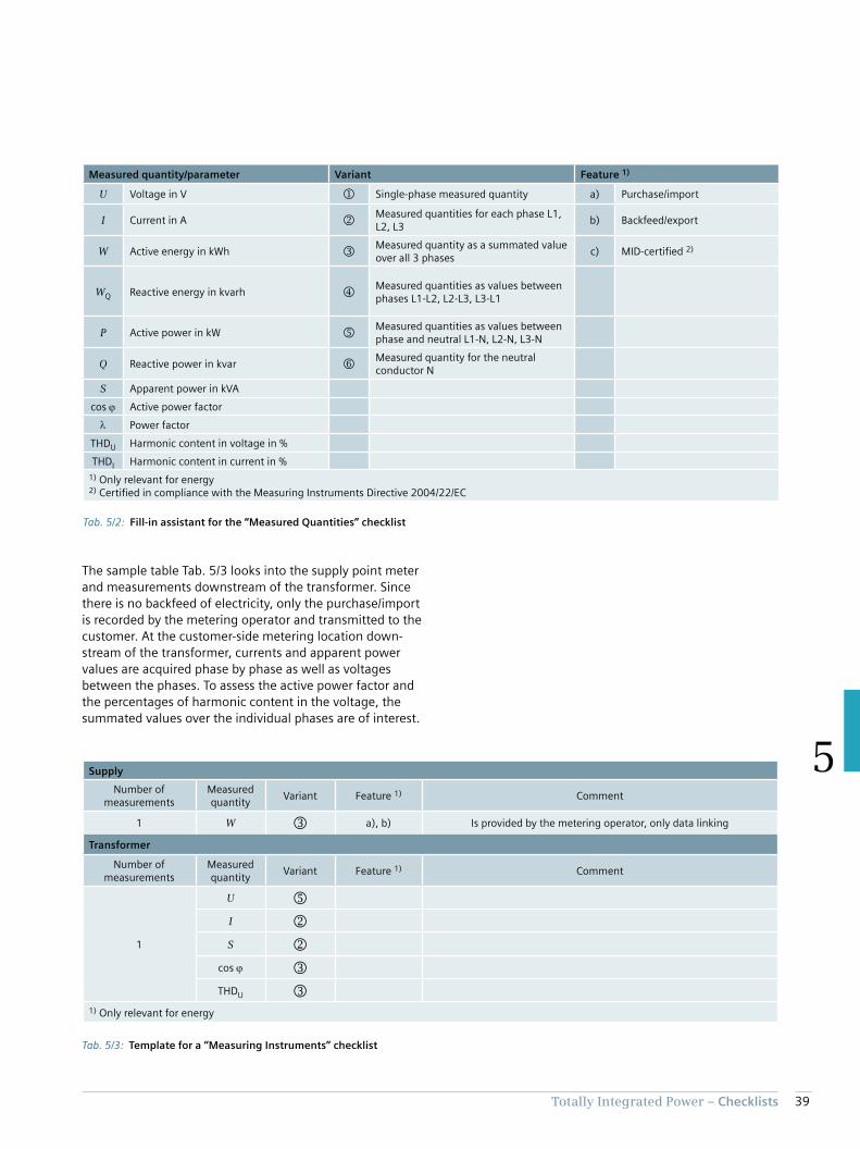
39Totally Integrated Power – Checklists
5
The sample table Tab. 5/3 looks into the supply point meter
and measurements downstream of the transformer. Since
there is no backfeed of electricity, only the purchase/import
is recorded by the metering operator and transmitted to the
customer. At the customer-side metering location down-
stream of the transformer, currents and apparent power
values are acquired phase by phase as well as voltages
between the phases. To assess the active power factor and
the percentages of harmonic content in the voltage, the
summated values over the individual phases are of interest.
Tab. 5/2: Fill-in assistant for the “Measured Quantities” checklist
Measured quantity/parameter Variant Feature 1)
U Voltage in V Single-phase measured quantity a) Purchase/import
I Current in AMeasured quantities for each phase L1, L2, L3
b) Backfeed/export
W Active energy in kWhMeasured quantity as a summated value over all 3 phases
c) MID-certified 2)
WQ Reactive energy in kvarhMeasured quantities as values between phases L1-L2, L2-L3, L3-L1
P Active power in kWMeasured quantities as values between phase and neutral L1-N, L2-N, L3-N
Q Reactive power in kvarMeasured quantity for the neutral conductor N
S Apparent power in kVA
cos Active power factor
Power factor
THDU Harmonic content in voltage in %
THDI Harmonic content in current in %
1) Only relevant for energy2) Certified in compliance with the Measuring Instruments Directive 2004/22/EC
Tab. 5/3: Template for a “Measuring Instruments” checklist
Supply
Number of measurements
Measured quantity
Variant Feature 1) Comment
1 W a), b) Is provided by the metering operator, only data linking
Transformer
Number of measurements
Measured quantity
Variant Feature 1) Comment
1
U
I
S
cos
THDU
1) Only relevant for energy

40 Totally Integrated Power – Checklists
5
5.2 “Graphics” checklist and “Tables” checklist
To select graphics to be chosen for illustration, a simple
matrix is sufficient (Tab. 5/4), where dots mark which
graphic forms of representation are used for the different
Tab. 5/4: Checklist for graphic analyses on controlling
Supply Transformer Generator Distribution Loads Tenants
Load profile
- Year
- Month
- Week
- Day
Frequency distribution
- Year
- Month
Utilization profile
- Year
- Month
Maxima evaluation
- Year / Maxima sequence
- Year / Day distribution
- Month / Maxima sequence
- Month / Day distribution
Tab. 5/5: Checklist for tabular analysis and the derived diagrams for controlling
Supply Transformer Generator Distribution Loads Tenants
Parameters, tabular
Power
Maximum values
Minimum values (arithmetic)
Minimum values
Energyabsolute
cumulated
Peak load share
Full load hours
...
Table values as graphics (bar charts, pie charts, ...)
Energy consumption and power peaks
Power per month
Maximum values
Minimum values (arithmetic)
Minimum values
Energy consumption
absolute
cumulated
...
levels of electric power distribution. Tables and associated
diagrammatic representations (bar charts, pie charts, or
dots diagrams) can be used for tabular analysis (Tab. 5/5).

Chapter 6Hardware and software for measured value acquisition and analysis
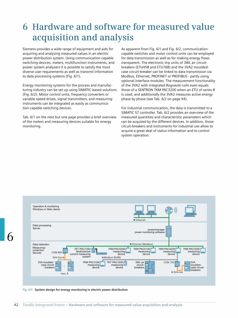
42 Totally Integrated Power – Hardware and software for measured value acquisition and analysis
6
6 Hardware and software for measured value acquisition and analysis
Siemens provides a wide range of equipment and aids for
acquiring and analysing measured values in an electric
power distribution system. Using communication-capable
switching devices, meters, multifunction instruments, and
power system analysers it is possible to satisfy the most
diverse user requirements as well as transmit information
to data processing systems (Fig. 6/1).
Energy monitoring systems for the process and manufac-
turing industry can be set up using SIMATIC-based solutions
(Fig. 6/2). Motor control units, frequency converters or
variable speed drives, signal transmitters, and measuring
instruments can be integrated as easily as communica-
tion-capable switching devices.
Tab. 6/1 on the next but one page provides a brief overview
of the meters and measuring devices suitable for energy
monitoring.
As apparent from Fig. 6/1 and Fig. 6/2, communication-
capable switches and motor control units can be employed
for data transmission as well as for making energy flows
transparent. The electronic trip units of 3WL air circuit-
breakers (ETU45B and ETU76B) and the 3VA2 moulded-
case circuit-breaker can be linked to data transmission via
Modbus, Ethernet, PROFINET or PROFIBUS - partly using
optional interface modules. The measurement functionality
of the 3VA2 with integrated Rogowski coils even equals
those of a SENTRON 7KM PAC3200 when an ETU of series 8
is used, and additionally the 3VA2 measures active energy
phase by phase (see Tab. 6/2 on page 44).
For industrial communication, the data is transmitted to a
SIMATIC S7 controller. Tab. 6/2 provides an overview of the
measured quantities and characteristic parameters which
can be acquired by the different devices. In addition, those
circuit-breakers and instruments for industrial use allow to
acquire a great deal of status information and to control
system operation.
Fig. 6/1: System design for energy monitoring in electric power distribution
3WL air circuit-
breakers
Measuring/protection devices
Data detection
ServerData processing
Windows or Web clientsOperation & monitoring
powermanager power monitoring software
7KT PAC1500 measuring
device
7KM PAC3100 measuring
device
7KM PAC3200 measuring
device
7KM PAC4200 measuring
device
7KM PAC5100 measuring
device
7KM PAC5200 measuring
device
3VA moulded- case circuit- breakers
3VA moulded-case circuit-
breakers
7KT PAC1200 Multichannel
current measuring system

43Totally Integrated Power – Hardware and software for measured value acquisition and analysis
6
Fig. 6/2: System design for energy monitoring in the process and manufacturing industry
...
SIMATIC S7
3VA-line3VA-line
3VA3VA
COM15
3VA
max. 8
PROFIBUS DP
PROFINET / PROFIenergy
Industrial Ethernet
PROFINET
3WL
COM800COM100
Industrial Ethernet
Distributed periphery, e.g. ET200
SINAMICS G120frequency converter
Operating and monitoring level
Data acquisition and control level
SIMATIC PCS 7 / WinCCOptions: powerrate and block library
Analogue and digital signals from contactors, counters and flow meters
SIMOCODEpro
motor management
system
Archive
Processing level
7KM PAC32007KM PAC4200
measuringdevices
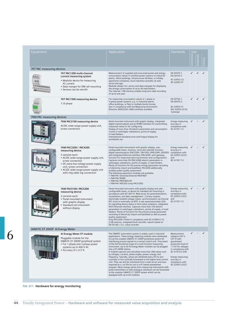
44 Totally Integrated Power – Hardware and software for measured value acquisition and analysis
6
Tab. 6/1: Hardware for energy monitoring
--
--
--
--
Equipment Application Standards Use
Co
mm
erc
ial
Re
sid
en
tia
l
Ind
ust
ry
7KM PAC3100 measuring device
AC/DC wide-range power supply unit, screw connection
Panel-mounted instrument with graphic display, integrated digital inputs/outputs and an RS485 interface for transmitting measured values or for configuring.Display of more than 30 electric parameters and consumption counts in switchgear substations, points of supply, or load feeders.International standards and multi-lingual display for worldwide use.
Energy measuring accuracy in compliance with IEC 61557-12
7KM PAC3200 / PAC4200 measuring device
3 variants each:• AC/DC wide-range power supply unit, screw connection• DC extra-low voltage power supply unit, screw connection• AC/DC wide-range power supply unit with ring cable lug connection
Energy measuring accuracy in compliance with IEC 62053-22/23andIEC 61557-12
7KT PAC1500 measuring device
1-/3-phase
For measuring consumption values in 1-phase or 3-phase power systems, e.g. in industrial plants, office buildings, or flats in multiple-family homes; also in compliance with the Measuring Instruments Directive 2004/22/EC (MID-certified) available.
EN 50740-1,EN 50470-3, IEC 62053-31(IEC 62052-23 für3-phasig)
Energy measuring accuracy in compliance with IEC 62053-22/23andIEC 61557-12
7KM PAC5100 / PAC5200measuring device
2 variants each:• Panel-mounted instrument with graphic display• Standard rail instrument without display
AI Energy Meter ST module
Pluggable module for the SIMATIC ET 200SP peripheral system• For 1-phase and 3-phase power systems up to 400 V AC• Accuracy of ± 0.5 %
The SIMATIC automation system is widely used in industrial applications. These energy metering modules were developed to suit the scalable SIMATIC ET 200SP peripheral system for interfacing process signals to a central control unit. They boast of the full functional scope of a multi-function measuring instrument. Up to 42 Al Energy Meter modules can be plugged into a ET 200SP station. A module captures and calculates more than 200 values such as voltages, currents, phase angles, power, energy, and frequency. Typically, values are refreshed every 50 ms and cyclically or non-cyclically forwarded to the higher-level control unit. They can also be monitored from a web server and even exported as a .csv file for use in a PC-based spreadsheet program. More energy values from measuring instruments with pulse transmitters or with analogue interfaces can be forwarded to the modular SIMATIC ET 200SP system which can be equipped with up to 64 modules.
Measurement category CAT II, CAT III with guaranteed protection level of 1.5 kV for voltages in compliance with IEC 61010-2-030
Energy measuring accuracy in compliance with IEC 62053-22/23
Panel-mounted instruments with graphic display, user-configurable views, memory, clock and calendar function, digital inputs/outputs (PAC3200: 1DI/1DO); (PAC4200: 2DI2DO) and integrated Ethernet interface (PAC4200: with gateway function for measured-value transmission and configuration). Captures more than 50 (PAC3200) electric parameters in switchgear substations, points of supply, or load feeders. Plenty of functions for the precise energy parameter recording of electricity import and backfeed, PAC4200 additionally enables power quality assessment.The following expansion modules are available:• 7KM PAC Switched Ethernet PROFINET• 7KM PAC RS485• 7KM PAC PROFIBUS DP• 7KM PAC 4DI/2DO (only PAC4200).
Panel-mounted instrument with graphic display and user-configurable views, or device for standard rail mounting in accordance with IEC 60715. Web server for parameterization, visualization, and data management. 2 binary outputs, electrically isolated voltage inputs, synchronization via internal RTC clock or externally via NTP, 4 user-parameterizable LEDs for signalling device status or limit-value violations, integrated RJ45 Ethernet interface. Captures more than 250 electric parameters in switchgear substations, points of supply, or load feeders. Plenty of functions for the precise energy parameter recording of electricity import and backfeed as well as power quality assessment.Only PAC5200: Flicker in compliance with IEC 61000-4-15, 2 GB memory, integrated fault recorder, reports based on EN 50160, r.m.s. value recorder.
7KM PAC measuring devices
7KT PAC measuring devices
SIMATIC ET 200SP AI Energy Meter
7KT PAC1200 multi-channel current measuring system
• Modular device for measuring AC current• Data manger for DIN rail mounting• Sensors can be retrofit
Measurement of supplied and consumed power and energy, consumption values in ramified power systems of industrial plants, office buildings, infrastructure facilities, or holiday apartment complexes; local indication possible via web server and app.Modular design incl. sensor and data manager for displaying the energy consumption of up to 96 load feeders.The internal 1-GB-memory enables long-term data recording of up to one year.
EN 50470-1,
EN 50470-3
IEC 62052-23,
IEC 62053-31
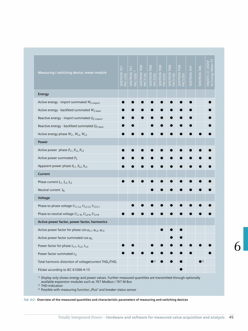
45Totally Integrated Power – Hardware and software for measured value acquisition and analysis
6
Tab. 6/2: Overview of the measured quantities and characteristic parameters of measuring and switching devices
2) 3)
SE
NT
RO
N 7
KT
PAC
12
00
SE
NT
RO
N 7
KT
PAC
15
00
1)
SE
NT
RO
N 7
KM
PAC
31
00
SE
NT
RO
N 7
KM
PAC
32
00
SE
NT
RO
N 7
KM
PAC
42
00
SE
NT
RO
N 7
KM
PAC
51
00
SE
NT
RO
N 7
KM
PAC
52
00
SE
NT
RO
N 3
VA
SE
NT
RO
N 3
WL
SIM
AT
IC E
T 2
00
SP
AI
En
erg
y M
ete
r S
T
Energy
Active energy - import summated W -import
Active energy - backfeed summated W -back
Reactive energy - import summated Q -import
Reactive energy - backfeed summated Q -back
Active energy phase WL1, WL2, WL3
Power
Active power phase PL1, PL2, PL3
Active power summated P
Apparent power phase SL1, SL2, SL3
Current
Phase current IL1, IL2, IL3
Neutral current IN
Voltage
Phase-to-phase voltage UL1-L2, UL2-L3, UL3-L1
Phase-to-neutral voltage UL1-N, UL2-N, UL3-N
Active power factor, power factor, harmonics
Active power factor for phase cos L1, L2, L3
Active power factor summated cos
Power factor for phase L1, L2, L3
Power factor summated
Total harmonic distortion of voltage/current THDU/THDI
Flicker according to IEC 61000-4-15
1) Display only shows energy and power values. Further measured quantities are transmitted through optionally available expansion modules such as 7KT Modbus / 7KT M-Bus2) THD-indication3) Possible with measuring function „Plus“ and breaker status sensor
Measuring / switching device, meter module
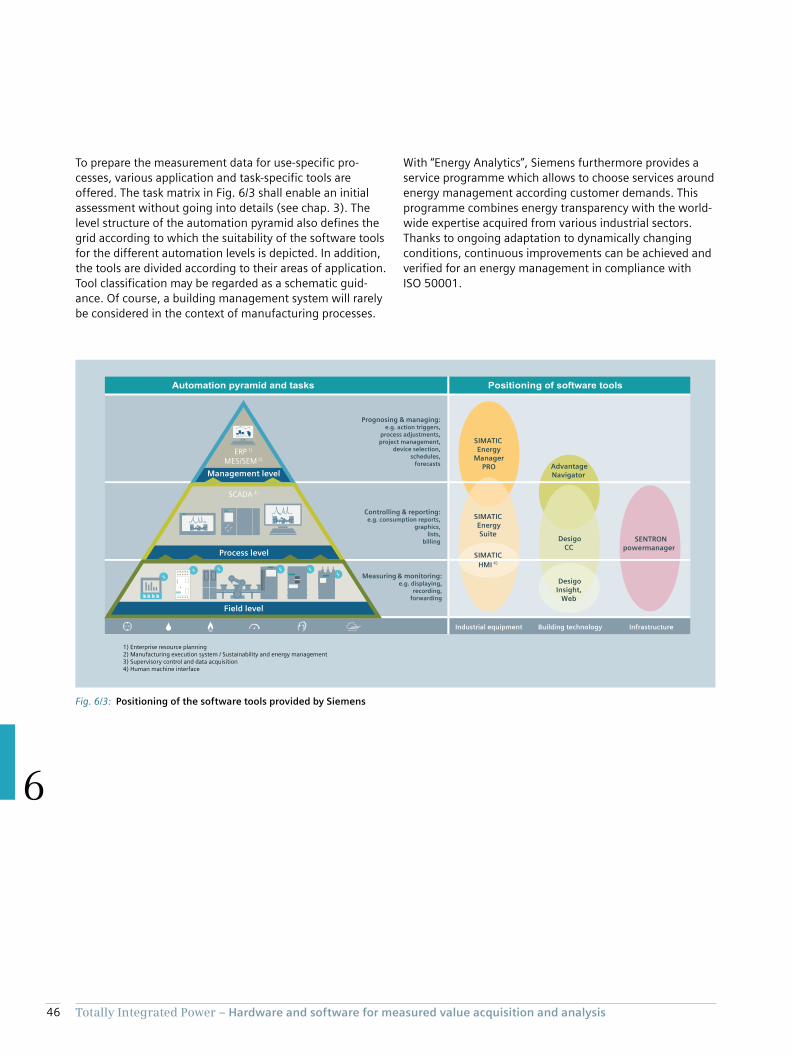
46 Totally Integrated Power – Hardware and software for measured value acquisition and analysis
6
To prepare the measurement data for use-specific pro-
cesses, various application and task-specific tools are
offered. The task matrix in Fig. 6/3 shall enable an initial
assessment without going into details (see chap. 3). The
level structure of the automation pyramid also defines the
grid according to which the suitability of the software tools
for the different automation levels is depicted. In addition,
the tools are divided according to their areas of application.
Tool classification may be regarded as a schematic guid-
ance. Of course, a building management system will rarely
be considered in the context of manufacturing processes.
With “Energy Analytics”, Siemens furthermore provides a
service programme which allows to choose services around
energy management according customer demands. This
programme combines energy transparency with the world-
wide expertise acquired from various industrial sectors.
Thanks to ongoing adaptation to dynamically changing
conditions, continuous improvements can be achieved and
verified for an energy management in compliance with
ISO 50001.
Fig. 6/3: Positioning of the software tools provided by Siemens
1) Enterprise resource planning2) Manufacturing execution system / Sustainability and energy management3) Supervisory control and data acquisition4) Human machine interface
MES/SEM 2)
ERP 1)
SCADA 3)
SIMATIC Energy
ManagerPRO
SIMATIC
HMI 4)
SIMATIC EnergySuite
DesigoCC
DesigoInsight,
Web
AdvantageNavigator
SENTRONpowermanager
Field level
Process level
Management level
Industrial equipment Building technology Infrastructure
Positioning of software tools
Measuring & monitoring:e.g. displaying,
recording,forwarding
Controlling & reporting:e.g. consumption reports,
graphics,lists,
billing
Prognosing & managing:e.g. action triggers,
process adjustments,project management,
device selection,schedules,
forecasts
Automation pyramid and tasks

Chapter 7Smart energy control for specific applications
7.1 Shopping centre 49
7.2 Data centre 50
7.3 Industrial plant 51
7.4 Supermarket 52
7.5 Distributed properties 53

48 Totally Integrated Power – Smart energy control for specific applications
7
7 Smart energy control for specific applications
Energy monitoring by way of measuring instruments which
enables energy flows to be controlled and adjusted using
appropriate analysis of the measurement data results in
energy efficiency improvements (see Tab. 7/1) entailing
• Operating cost reductions
• Increase of plant availability
• Efficiency improvements in engineering
The examples of Fig. 7/1 to Fig. 7/5 on the following pages
demonstrate methods of controlling through the creation
of energy transparency (see the draft of the German VDI
guideline VDI 2166 Sheet 1) as detailed below:
• Shopping centre
• Data centre
• Industrial plant
• Supermarket
• Distributed properties
Tab. 7/1: Customer benefits achieved by energy transparency
Energy transparency leads to:
Operating cost reductions by Increased plant availability by Efficient engineering by
Supporting the energy purchaser Maximizing operating timesParameterization instead of software programming
Profiting from lower demand charges Avoiding overload situations Time and cost savings by using software options
Improving energy cost awareness Optimizing maintenance expenses Integration into TIA and TIP
Optimizing capital investment Assured power quality by continuous monitoring and analysis
No redundant data storage
Identifying energy-intensive equipment Avoiding isolated information isles
Design based on standard system interfaces
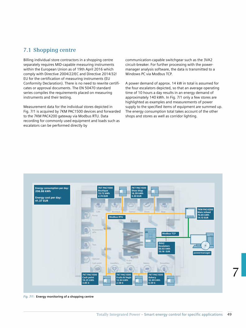
49Totally Integrated Power – Smart energy control for specific applications
7
7.1 Shopping centre
Billing individual store contractors in a shopping centre
separately requires MID-capable measuring instruments
within the European Union as of 19th April 2016 which
comply with Directive 2004/22/EC and Directive 2014/32/
EU for the certification of measuring instruments (EU
Conformity Declaration). There is no need to rewrite certifi-
cates or approval documents. The EN 50470 standard
series compiles the requirements placed on measuring
instruments and their testing.
Measurement data for the individual stores depicted in
Fig. 7/1 is acquired by 7KM PAC1500 devices and forwarded
to the 7KM PAC4200 gateway via Modbus RTU. Data
recording for commonly used equipment and loads such as
escalators can be performed directly by
communication-capable switchgear such as the 3VA2
circuit-breaker. For further processing with the power-
manager analysis software, the data is transmitted to a
Windows PC via Modbus TCP.
A power demand of approx. 14 kW in total is assumed for
the four escalators depicted, so that an average operating
time of 10 hours a day results in an energy demand of
approximately 140 kWh. In Fig. 7/1 only a few stores are
highlighted as examples and measurements of power
supply to the specified items of equipment are summed up.
The energy consumption total takes account of the other
shops and stores as well as corridor lighting.
Fig. 7/1: Energy monitoring of a shopping centre
Accessories/gifts
Cash point Bakery
Optician
Boutique Shoes Bags
Florist
Smoothies
Cafe
Fruits/VegisJuwellery
Fashion
Toys
Accessories/gifts
Cash point Bakery
Optician
iqueBoutique Shoes BagsBags
Florist
thiesSmoothies
Cafe
Fruits/VegisVegisJuwelleryJuwellery
ionFashion
Toys
powermanager
Modbus TCP
Modbus RTU
Energy consumption per day:
206.86 kWh
Energy cost per day:41.37 EUR
3VA2 Escalators50.92 kWh10.18 EUR
7KT PAC1500 Boutique13.72 kWh2.74 EUR
7KT PAC1500 Shoe shop16.39 kWh3.30 EUR
7KM PAC4200 Main infeed70.65 kWh14.13 EUR
7KT PAC1500 Cash point19.25 kWh3.85 €
7KT PAC1500 Fruits & Vegis12.94 kWh2.58 €
7KT PAC1500 Bakery32.99 kWh6.59 €
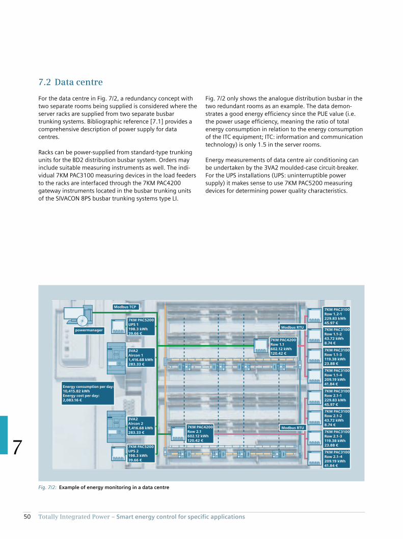
50 Totally Integrated Power – Smart energy control for specific applications
7
7.2 Data centre
For the data centre in Fig. 7/2, a redundancy concept with
two separate rooms being supplied is considered where the
server racks are supplied from two separate busbar
trunking systems. Bibliographic reference [7.1] provides a
comprehensive description of power supply for data
centres.
Racks can be power-supplied from standard-type trunking
units for the BD2 distribution busbar system. Orders may
include suitable measuring instruments as well. The indi-
vidual 7KM PAC3100 measuring devices in the load feeders
to the racks are interfaced through the 7KM PAC4200
gateway instruments located in the busbar trunking units
of the SIVACON 8PS busbar trunking systems type LI.
Fig. 7/2 only shows the analogue distribution busbar in the
two redundant rooms as an example. The data demon-
strates a good energy efficiency since the PUE value (i.e.
the power usage efficiency, meaning the ratio of total
energy consumption in relation to the energy consumption
of the ITC equipment; ITC: information and communication
technology) is only 1.5 in the server rooms.
Energy measurements of data centre air conditioning can
be undertaken by the 3VA2 moulded-case circuit-breaker.
For the UPS installations (UPS: uninterruptible power
supply) it makes sense to use 7KM PAC5200 measuring
devices for determining power quality characteristics.
Fig. 7/2: Example of energy monitoring in a data centre
Energy consumption per day:10,415.82 kWhEnergy cost per day:2,083.16 €
3VA2 Aircon 11,416.68 kWh283.33 €
7KM PAC5200UPS 1198.3 kWh39.66 €
3VA2 Aircon 21,416.68 kWh283.33 €
7KM PAC5200UPS 2198.3 kWh39.66 €
7KM PAC3100 Row 1.2-1229.83 kWh45.97 €
7KM PAC3100 Row 1.1-243.72 kWh8.74 €
7KM PAC3100 Row 1.1-3119.38 kWh23.88 €
7KM PAC3100 Row 2.1-1229.83 kWh45.97 €
7KM PAC3100 Row 2.1-243.72 kWh8.74 €
7KM PAC3100 Row 2.1-3119.38 kWh23.88 €
7KM PAC3100 Row 2.1-4209.19 kWh41.84 €
7KM PAC4200 Row 2.1602.12 kWh120.42 €
7KM PAC4200 Row 1.1602.12 kWh120.42 €
7KM PAC3100 Row 1.1-4209.19 kWh41.84 €
Modbus TCP
powermanagerModbus RTU
Modbus RTU
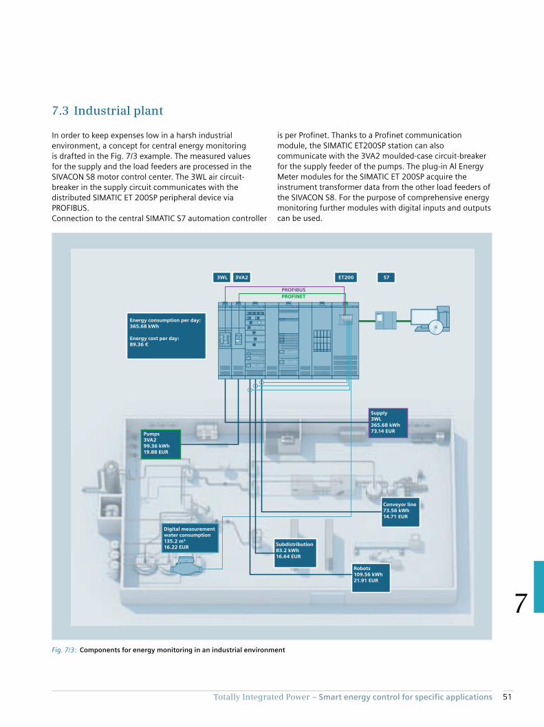
51Totally Integrated Power – Smart energy control for specific applications
7
7.3 Industrial plant
In order to keep expenses low in a harsh industrial
environment, a concept for central energy monitoring
is drafted in the Fig. 7/3 example. The measured values
for the supply and the load feeders are processed in the
SIVACON S8 motor control center. The 3WL air circuit-
breaker in the supply circuit communicates with the
distributed SIMATIC ET 200SP peripheral device via
PROFIBUS.
Connection to the central SIMATIC S7 automation controller
is per Profinet. Thanks to a Profinet communication
module, the SIMATIC ET200SP station can also
communicate with the 3VA2 moulded-case circuit-breaker
for the supply feeder of the pumps. The plug-in Al Energy
Meter modules for the SIMATIC ET 200SP acquire the
instrument transformer data from the other load feeders of
the SIVACON S8. For the purpose of comprehensive energy
monitoring further modules with digital inputs and outputs
can be used.
Fig. 7/3: Components for energy monitoring in an industrial environment
Energy consumption per day:365.68 kWh
Energy cost per day:89.36 €
Pumps 3VA299.36 kWh19.88 EUR
Subdistribution83.2 kWh16.64 EUR
Conveyor line73.56 kWh14.71 EUR
Supply3WL365.68 kWh73.14 EUR
Robots109.56 kWh21.91 EUR
Digital measurementwater consumption135.2 m³16.22 EUR
S7ET200
PROFINET
PROFIBUS
3VA23WL
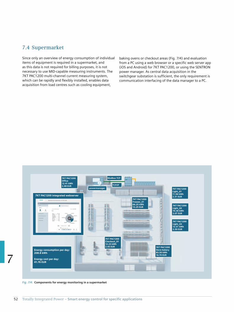
52 Totally Integrated Power – Smart energy control for specific applications
7
7.4 Supermarket
Since only an overview of energy consumption of individual
items of equipment is required in a supermarket, and
as this data is not required for billing purposes, it is not
necessary to use MID-capable measuring instruments. The
7KT PAC1200 multi-channel current measuring system,
which can be rapidly and flexibly installed, enables data
acquisition from load centres such as cooling equipment,
baking ovens or checkout areas (Fig. 7/4) and evaluation
from a PC using a web browser or a specific web server app
(iOS and Android) for 7KT PAC1200, or using the SENTRON
power manager. As central data acquisition in the
switchgear substation is sufficient, the only requirement is
communication interfacing of the data manager to a PC.
Fig. 7/4: Components for energy monitoring in a supermarket
Modbus TCP
TCP/IP
powermanager
7KT PAC1200 Checkout_0112.23 kWh2.45 EUR
7KT PAC1200 Office 12.41 kWh2.48 EUR
7KT PAC1200 Freezer_0166.25 kWh13.25 EUR
7KT PAC1200 Light_0210.36 kWh2.07 EUR
7KT PAC1200 Light_0312.51 kWh2.50 EUR
7KT PAC1200 Store bakery83.50 kWh16.70 EUR
7KT PAC1200 Light_0111.56 kWh2.31 EUR
7KT PAC1200 integrated webserver
Energy consumption per day:208.8 kWh
Energy cost per day:41.76 EUR
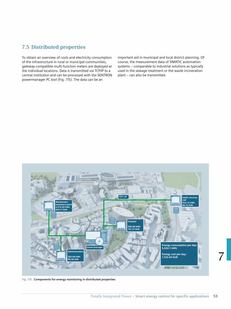
53Totally Integrated Power – Smart energy control for specific applications
7
7.5 Distributed properties
To obtain an overview of costs and electricity consumption
of the infrastructure in rural or municipal communities,
gateway-compatible multi-function meters are deployed at
the individual locations. Data is transmitted via TCP/IP to a
central institution and can be processed with the SENTRON
powermanager PC tool (Fig. 7/5). The data can be an
important aid in municipal and local district planning. Of
course, the measurement data of SIMATIC automation
systems ‒ comparable to industrial solutions as typically
used in the sewage treatment or the waste incineration
plant ‒ can also be transmitted.
Fig. 7/5: Components for energy monitoring in distributed properties
Energy consumption per day:5,532.1 kWh
Energy cost per day:1,122.64 EUR
Wastewater treatment plant4,215.83 kWh843.17 EUR
Administration
365.68 kWh89.36 EUR
Hospital
506.86 kWh101.37 EUR
Public servicesCHP443.72 kWh88.74 EUR
powermanager
TCP / IP

54 Totally Integrated Power – Smart energy control for specific applications
7

Chapter 8Annex
8.1 Value ranges for energy consumption and power demand 56
8.2 Abbreviations 62
8.3 Formula symbols 62
8.4 Bibliography 63
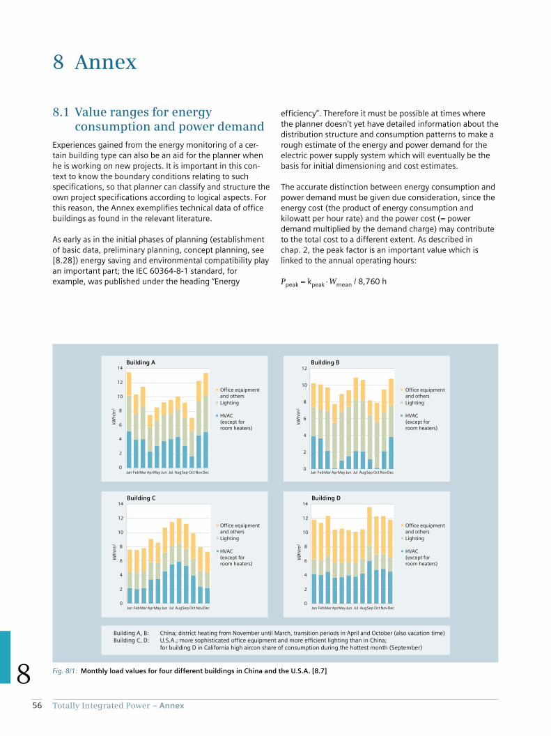
56 Totally Integrated Power – Annex
8
8 Annex
8.1 Value ranges for energy consumption and power demand
Experiences gained from the energy monitoring of a cer-
tain building type can also be an aid for the planner when
he is working on new projects. It is important in this con-
text to know the boundary conditions relating to such
specifications, so that planner can classify and structure the
own project specifications according to logical aspects. For
this reason, the Annex exemplifies technical data of office
buildings as found in the relevant literature.
As early as in the initial phases of planning (establishment
of basic data, preliminary planning, concept planning, see
[8.28]) energy saving and environmental compatibility play
an important part; the IEC 60364-8-1 standard, for
example, was published under the heading “Energy
efficiency”. Therefore it must be possible at times where
the planner doesn’t yet have detailed information about the
distribution structure and consumption patterns to make a
rough estimate of the energy and power demand for the
electric power supply system which will eventually be the
basis for initial dimensioning and cost estimates.
The accurate distinction between energy consumption and
power demand must be given due consideration, since the
energy cost (the product of energy consumption and
kilowatt per hour rate) and the power cost (= power
demand multiplied by the demand charge) may contribute
to the total cost to a different extent. As described in
chap. 2, the peak factor is an important value which is
linked to the annual operating hours:
Ppeak = kpeak · Wmean / 8,760 h
Fig. 8/1: Monthly load values for four different buildings in China and the U.S.A. [8.7]
0
2
4
6
8
10
12
14
kWh
/m2
kWh
/m2
kWh
/m2
kWh
/m2
0
2
4
6
8
10
12
0
2
4
6
8
10
12
14
0
2
4
6
8
10
12
14
Jan FebMar AprMay Jun Jul AugSep Oct NovDec
Building A
Office equipment and others
Lighting
HVAC (except for room heaters)
Jan FebMar AprMay Jun Jul AugSep Oct NovDec
Building B
Jan FebMar AprMay Jun Jul AugSep Oct NovDec
Building C
Jan FebMar AprMay Jun Jul AugSep Oct NovDec
Building D
Building A, B: China; district heating from November until March, transition periods in April and October (also vacation time)Building C, D: U.S.A.; more sophisticated office equipment and more efficient lighting than in China; for building D in California high aircon share of consumption during the hottest month (September)
Office equipment and others
Lighting
HVAC (except for room heaters)
Office equipment and others
Lighting
HVAC (except for room heaters)
Office equipment and others
Lighting
HVAC (except for room heaters)
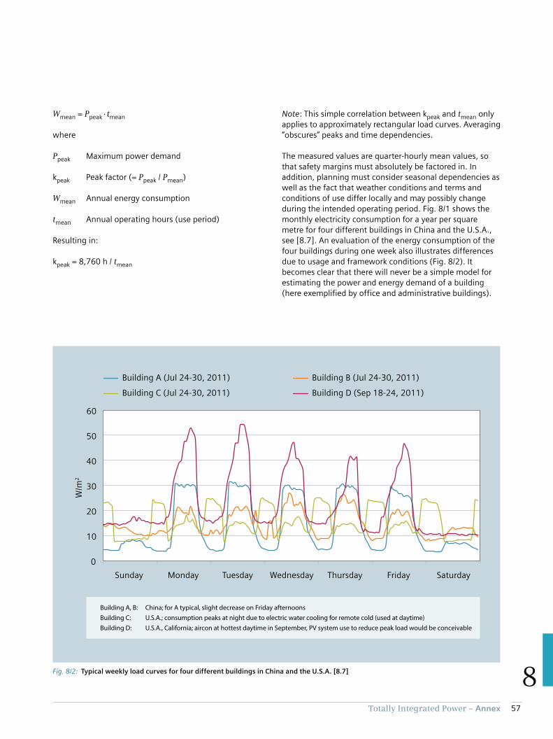
57Totally Integrated Power – Annex
8
Wmean = Ppeak · tmean
where
Ppeak Maximum power demand
kpeak Peak factor (= Ppeak / Pmean)
Wmean Annual energy consumption
tmean Annual operating hours (use period)
Resulting in:
kpeak = 8,760 h / tmean
Note: This simple correlation between kpeak and tmean only
applies to approximately rectangular load curves. Averaging
“obscures” peaks and time dependencies.
The measured values are quarter-hourly mean values, so
that safety margins must absolutely be factored in. In
addition, planning must consider seasonal dependencies as
well as the fact that weather conditions and terms and
conditions of use differ locally and may possibly change
during the intended operating period. Fig. 8/1 shows the
monthly electricity consumption for a year per square
metre for four different buildings in China and the U.S.A.,
see [8.7]. An evaluation of the energy consumption of the
four buildings during one week also illustrates differences
due to usage and framework conditions (Fig. 8/2). It
becomes clear that there will never be a simple model for
estimating the power and energy demand of a building
(here exemplified by office and administrative buildings).
Fig. 8/2: Typical weekly load curves for four different buildings in China and the U.S.A. [8.7]
0
10
20
30
40
50
60
W/m
2
Building A (Jul 24-30, 2011) Building B (Jul 24-30, 2011)
Building C (Jul 24-30, 2011) Building D (Sep 18-24, 2011)
Sunday Monday SaturdayFridayThursdayWednesdayTuesday
Building A, B: China; for A typical, slight decrease on Friday afternoons
Building C: U.S.A.; consumption peaks at night due to electric water cooling for remote cold (used at daytime)
Building D: U.S.A., California; aircon at hottest daytime in September, PV system use to reduce peak load would be conceivable
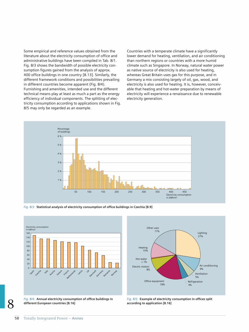
58 Totally Integrated Power – Annex
8
Some empirical and reference values obtained from the
literature about the electricity consumption of office and
administrative buildings have been compiled in Tab. 8/1.
Fig. 8/3 shows the bandwidth of possible electricity con-
sumption figures gained from the analysis of approx.
400 office buildings in one country [8.13]. Similarly, the
different framework conditions and possibilities prevailing
in different countries become apparent (Fig. 8/4).
Furnishing and amenities, intended use and the different
technical means play at least as much a part as the energy
efficiency of individual components. The splitting of elec-
tricity consumption according to applications shown in Fig.
8/5 may only be regarded as an example.
Fig. 8/3: Statistical analysis of electricity consumption of office buildings in Czechia [8.9]
50 450400350300250200150100
1 %
5 %
4 %
3 %
2 %
6 %
Electricity consumptionin kWh/m2
Percentage of buildings
Countries with a temperate climate have a significantly
lower demand for heating, ventilation, and air conditioning
than northern regions or countries with a more humid
climate such as Singapore. In Norway, natural water power
as native source of electricity is also used for heating,
whereas Great Britain uses gas for this purpose, and in
Germany a mix consisting largely of oil, gas, wood, and
electricity is also used for heating. It is, however, conceiv-
able that heating and hot-water preparation by means of
electricity will experience a renaissance due to renewable
electricity generation.
Fig. 8/4: Annual electricity consumption of office buildings in
different European countries [8.16]
0
20
40
60
80
100
120
140
160
Electricity consumption in kWh/m2
Spai
n
Czech
ia
Roman
ia
Germ
any
Denm
ark
Latv
ia UK
Nether
lands
Fran
ce
Greec
e
Austria
Italy
Norway
Fig. 8/5: Example of electricity consumption in offices split
according to application [8.16]
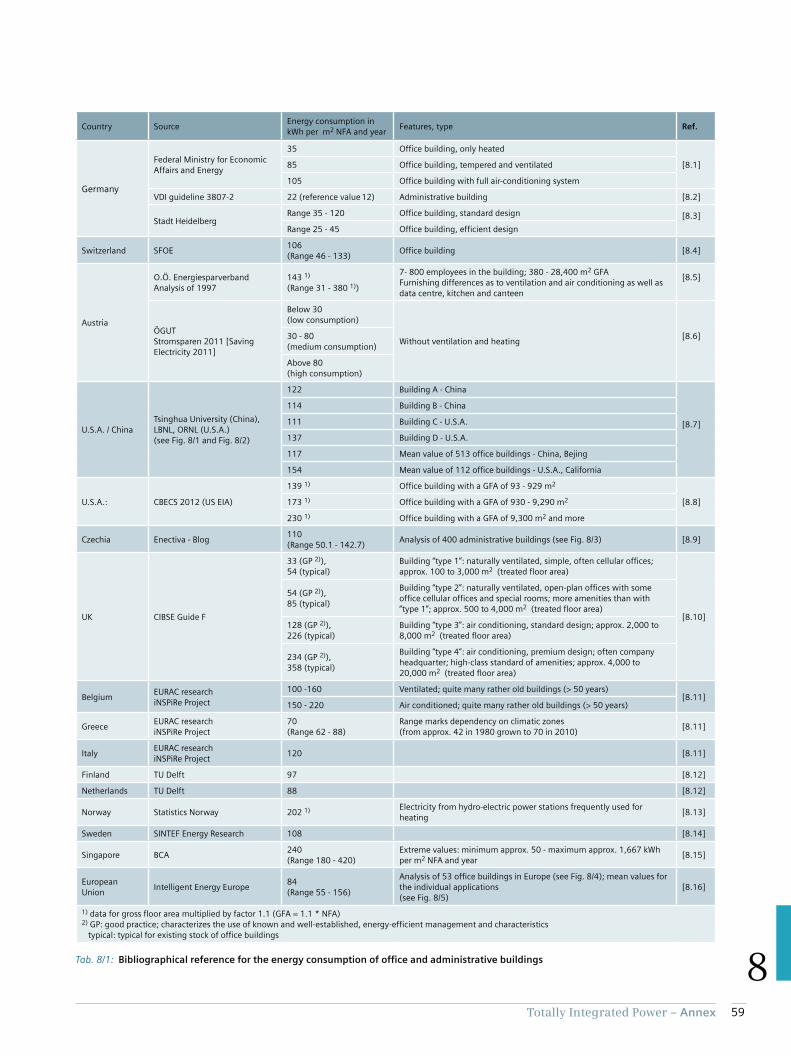
59Totally Integrated Power – Annex
8Tab. 8/1: Bibliographical reference for the energy consumption of office and administrative buildings
Country SourceEnergy consumption in kWh per m2 NFA and year
Features, type Ref.
Germany
Federal Ministry for Economic Affairs and Energy
35 Office building, only heated
[8.1]85 Office building, tempered and ventilated
105 Office building with full air-conditioning system
VDI guideline 3807-2 22 (reference value 12) Administrative building [8.2]
Stadt HeidelbergRange 35 - 120 Office building, standard design [8.3]
Range 25 - 45 Office building, efficient design
Switzerland SFOE106 (Range 46 - 133)
Office building [8.4]
Austria
O.Ö. Energiesparverband Analysis of 1997
143 1) (Range 31 - 380 1))
7- 800 employees in the building; 380 - 28,400 m2 GFAFurnishing differences as to ventilation and air conditioning as well as data centre, kitchen and canteen
[8.5]
ÖGUT Stromsparen 2011 [Saving Electricity 2011]
Below 30 (low consumption)
Without ventilation and heating[8.6]30 - 80
(medium consumption)
Above 80 (high consumption)
U.S.A. / ChinaTsinghua University (China), LBNL, ORNL (U.S.A.) (see Fig. 8/1 and Fig. 8/2)
122 Building A - China
[8.7]
114 Building B - China
111 Building C - U.S.A.
137 Building D - U.S.A.
117 Mean value of 513 office buildings - China, Bejing
154 Mean value of 112 office buildings - U.S.A., California
U.S.A.: CBECS 2012 (US EIA)
139 1) Office building with a GFA of 93 - 929 m2
[8.8]173 1) Office building with a GFA of 930 - 9,290 m2
230 1) Office building with a GFA of 9,300 m2 and more
Czechia Enectiva - Blog110 (Range 50.1 - 142.7)
Analysis of 400 administrative buildings (see Fig. 8/3) [8.9]
UK CIBSE Guide F
33 (GP 2)), 54 (typical)
Building “type 1”: naturally ventilated, simple, often cellular offices; approx. 100 to 3,000 m2 (treated floor area)
[8.10]
54 (GP 2)), 85 (typical)
Building “type 2”: naturally ventilated, open-plan offices with some office cellular offices and special rooms; more amenities than with “type 1”; approx. 500 to 4,000 m2 (treated floor area)
128 (GP 2)), 226 (typical)
Building “type 3”: air conditioning, standard design; approx. 2,000 to 8,000 m2 (treated floor area)
234 (GP 2)), 358 (typical)
Building “type 4”: air conditioning, premium design; often company headquarter; high-class standard of amenities; approx. 4,000 to 20,000 m2 (treated floor area)
BelgiumEURAC research iNSPiRe Project
100 -160 Ventilated; quite many rather old buildings (> 50 years)[8.11]
150 - 220 Air conditioned; quite many rather old buildings (> 50 years)
GreeceEURAC research iNSPiRe Project
70(Range 62 - 88)
Range marks dependency on climatic zones (from approx. 42 in 1980 grown to 70 in 2010)
[8.11]
ItalyEURAC research iNSPiRe Project
120 [8.11]
Finland TU Delft 97 [8.12]
Netherlands TU Delft 88 [8.12]
Norway Statistics Norway 202 1) Electricity from hydro-electric power stations frequently used for heating
[8.13]
Sweden SINTEF Energy Research 108 [8.14]
Singapore BCA240 (Range 180 - 420)
Extreme values: minimum approx. 50 - maximum approx. 1,667 kWh per m2 NFA and year
[8.15]
European Union
Intelligent Energy Europe84 (Range 55 - 156)
Analysis of 53 office buildings in Europe (see Fig. 8/4); mean values for the individual applications (see Fig. 8/5)
[8.16]
1) data for gross floor area multiplied by factor 1.1 (GFA = 1.1 * NFA)2) GP: good practice; characterizes the use of known and well-established, energy-efficient management and characteristics typical: typical for existing stock of office buildings
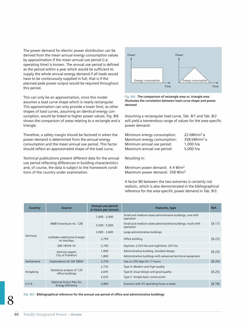
60 Totally Integrated Power – Annex
8
The power demand for electric power distribution can be
derived from the mean annual energy consumption values
by approximation if the mean annual use period (i.e.
operating time) is known. The annual use period is defined
as the period within a year which would be sufficient to
supply the whole annual energy demand if all loads would
have to be continuously supplied in full, that is if the
planned peak power output would be required throughout
this period.
This can only be an approximation, since this model
assumes a load curve shape which is nearly rectangular.
This approximation can only provide a lower limit, as other
shapes of load curves, assuming an identical energy con-
sumption, would be linked to higher power values. Fig. 8/6
shows the comparison of areas relating to a rectangle and a
triangle.
Therefore, a safety margin should be factored in when the
power demand is determined from the annual energy
consumption and the mean annual use period. This factor
should reflect an approximated shape of the load curve.
Technical publications present different data for the annual
use period reflecting differences in building characteristics
and, of course, the data is subject to the framework condi-
tions of the country under examination.
Tab. 8/2: Bibliographical reference for the annual use period of office and administrative buildings
Country SourceAnnual use period
in hours per annumFeatures, type Ref.
Germany
AMEV brochure no. 128
1,000 - 2,000Small and medium-sized administrative buildings; one-shift operation
[8.17]3,500 - 5,000
Small and medium-sized administrative buildings; multi-shift operation
2,000 - 2,600 Large administrative buildings
Leitfaden elektrische Energie im Hochbau
2,750 Office building [8.22]
DIN 18559-10 2,750 Daytime: 2,543 h/a and nighttime: 207 h/a
Seminar papers City of Frankfurt
1,000 Administrative building, standard design [8.23]
1,800 Administrative buildings with advanced technical equipment
Switzerland Explanations for SIA 380/4 2,750 Use on 250 days for 11 hours [8.24]
HongkongStatistical analysis of 120
office buildings
2,732 Type A: Modern and high quality
[8.25]2,645 Type B: Usual design and good quality
2,635 Type C: Simple basic construction
U.S.A.National Action Plan for
Energy Efficiency2,860 Scenario with 55 operating hours a week [8.18]
Assuming a rectangular load curve, Tab. 8/1 and Tab. 8/2
will yield a tremendous range of values for the area-specific
power demand:
Minimum energy consumption: 22 kWh/m2 a
Maximum energy consumption: 358 kWh/m2 a
Minimum annual use period: 1,000 h/a
Maximum annual use period: 5,000 h/a
Resulting in:
Minimum power demand: 4.4 W/m2
Maximum power demand: 358 W/m2
A factor 80 between the two extremes is certainly not
realistic, which is also demonstrated in the bibliographical
reference for the area-specific power demand in Tab. 8/3.
Fig. 8/6: The comparison of rectangle area vs. triangle area
illustrates the correlation between load curve shape and power
demand
Energy consumption Energy consumption
TimeTime
PowerPower
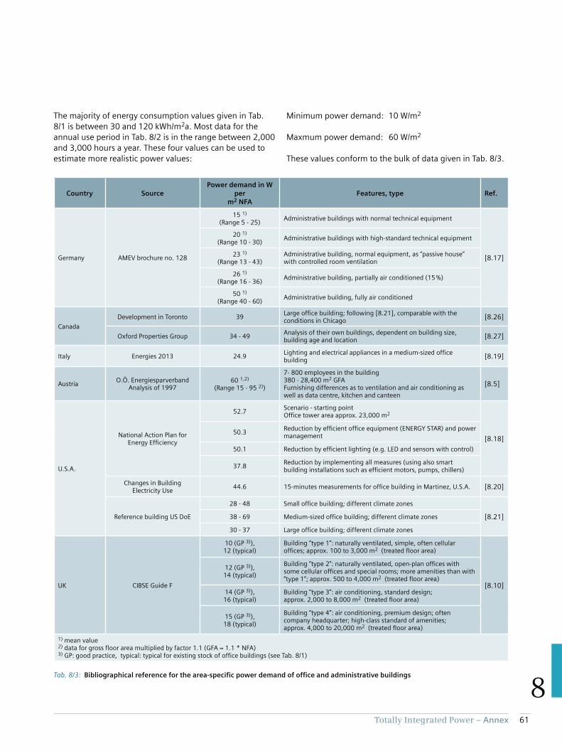
61Totally Integrated Power – Annex
8
The majority of energy consumption values given in Tab.
8/1 is between 30 and 120 kWh/m2a. Most data for the
annual use period in Tab. 8/2 is in the range between 2,000
and 3,000 hours a year. These four values can be used to
estimate more realistic power values:
Tab. 8/3: Bibliographical reference for the area-specific power demand of office and administrative buildings
Country SourcePower demand in W
per m2 NFA
Features, type Ref.
Germany AMEV brochure no. 128
15 1) (Range 5 - 25)
Administrative buildings with normal technical equipment
[8.17]
20 1) (Range 10 - 30)
Administrative buildings with high-standard technical equipment
23 1) (Range 13 - 43)
Administrative building, normal equipment, as “passive house” with controlled room ventilation
26 1) (Range 16 - 36)
Administrative building, partially air conditioned (15 %)
50 1) (Range 40 - 60)
Administrative building, fully air conditioned
Canada
Development in Toronto 39Large office building; following [8.21], comparable with the conditions in Chicago
[8.26]
Oxford Properties Group 34 - 49Analysis of their own buildings, dependent on building size, building age and location
[8.27]
Italy Energies 2013 24.9 Lighting and electrical appliances in a medium-sized office building
[8.19]
AustriaO.Ö. Energiesparverband
Analysis of 199760 1,2)
(Range 15 - 95 2))
7- 800 employees in the building380 - 28,400 m2 GFAFurnishing differences as to ventilation and air conditioning as well as data centre, kitchen and canteen
[8.5]
U.S.A.
National Action Plan for Energy Efficiency
52.7Scenario - starting pointOffice tower area approx. 23,000 m2
[8.18]50.3
Reduction by efficient office equipment (ENERGY STAR) and power management
50.1 Reduction by efficient lighting (e.g. LED and sensors with control)
37.8Reduction by implementing all measures (using also smart building installations such as efficient motors, pumps, chillers)
Changes in Building Electricity Use
44.6 15-minutes measurements for office building in Martinez, U.S.A. [8.20]
Reference building US DoE
28 - 48 Small office building; different climate zones
[8.21]38 - 69 Medium-sized office building; different climate zones
30 - 37 Large office building; different climate zones
UK CIBSE Guide F
10 (GP 3)), 12 (typical)
Building “type 1”: naturally ventilated, simple, often cellular offices; approx. 100 to 3,000 m2 (treated floor area)
[8.10]
12 (GP 3)), 14 (typical)
Building “type 2”: naturally ventilated, open-plan offices with some cellular offices and special rooms; more amenities than with “type 1”; approx. 500 to 4,000 m2 (treated floor area)
14 (GP 3)), 16 (typical)
Building “type 3”: air conditioning, standard design; approx. 2,000 to 8,000 m2 (treated floor area)
15 (GP 3)), 18 (typical)
Building “type 4”: air conditioning, premium design; often company headquarter; high-class standard of amenities; approx. 4,000 to 20,000 m2 (treated floor area)
1) mean value 2) data for gross floor area multiplied by factor 1.1 (GFA = 1.1 * NFA)3) GP: good practice, typical: typical for existing stock of office buildings (see Tab. 8/1)
Minimum power demand: 10 W/m2
Maxmum power demand: 60 W/m2
These values conform to the bulk of data given in Tab. 8/3.
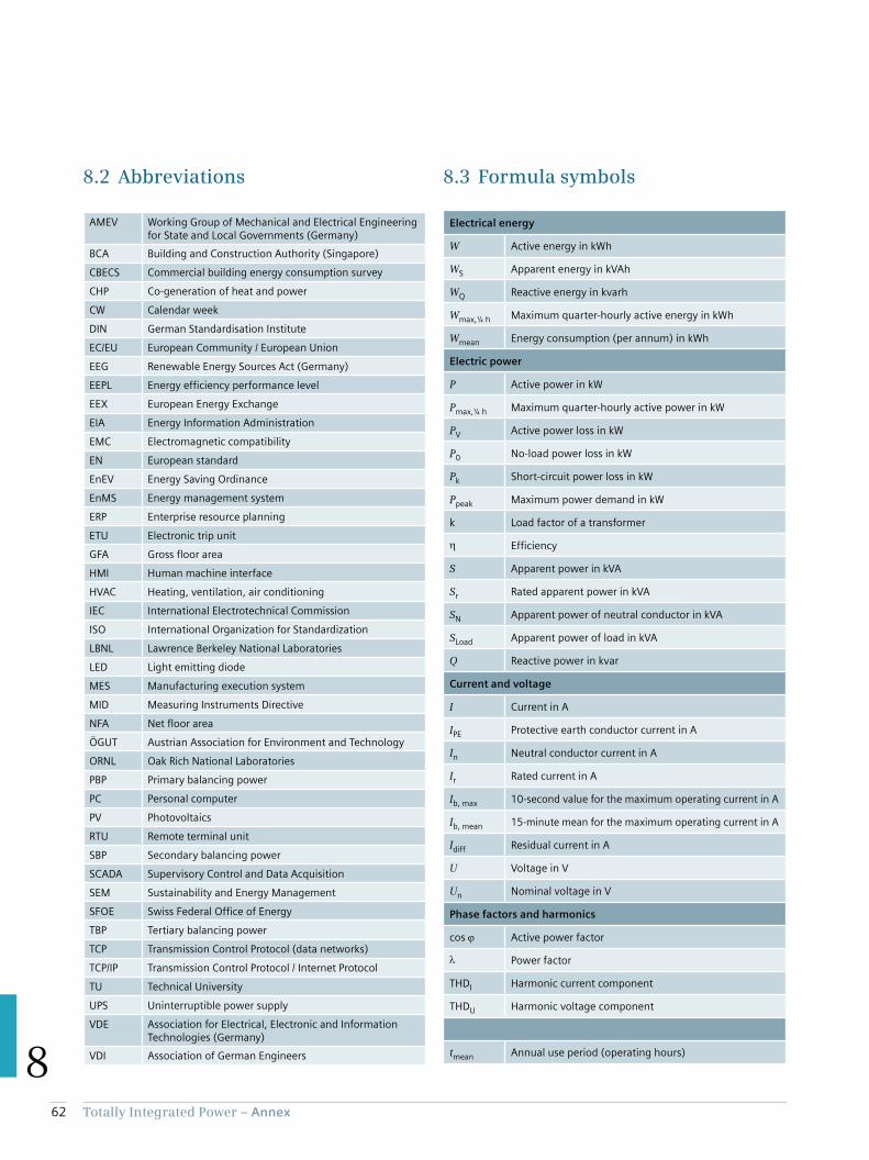
62 Totally Integrated Power – Annex
8
8.2 Abbreviations
AMEV Working Group of Mechanical and Electrical Engineering for State and Local Governments (Germany)
BCA Building and Construction Authority (Singapore)
CBECS Commercial building energy consumption survey
CHP Co-generation of heat and power
CW Calendar week
DIN German Standardisation Institute
EC/EU European Community / European Union
EEG Renewable Energy Sources Act (Germany)
EEPL Energy efficiency performance level
EEX European Energy Exchange
EIA Energy Information Administration
EMC Electromagnetic compatibility
EN European standard
EnEV Energy Saving Ordinance
EnMS Energy management system
ERP Enterprise resource planning
ETU Electronic trip unit
GFA Gross floor area
HMI Human machine interface
HVAC Heating, ventilation, air conditioning
IEC International Electrotechnical Commission
ISO International Organization for Standardization
LBNL Lawrence Berkeley National Laboratories
LED Light emitting diode
MES Manufacturing execution system
MID Measuring Instruments Directive
NFA Net floor area
ÖGUT Austrian Association for Environment and Technology
ORNL Oak Rich National Laboratories
PBP Primary balancing power
PC Personal computer
PV Photovoltaics
RTU Remote terminal unit
SBP Secondary balancing power
SCADA Supervisory Control and Data Acquisition
SEM Sustainability and Energy Management
SFOE Swiss Federal Office of Energy
TBP Tertiary balancing power
TCP Transmission Control Protocol (data networks)
TCP/IP Transmission Control Protocol / Internet Protocol
TU Technical University
UPS Uninterruptible power supply
VDE Association for Electrical, Electronic and Information Technologies (Germany)
VDI Association of German Engineers
Electrical energy
W Active energy in kWh
WS Apparent energy in kVAh
WQ Reactive energy in kvarh
Wmax,¼ h Maximum quarter-hourly active energy in kWh
Wmean Energy consumption (per annum) in kWh
Electric power
P Active power in kW
Pmax,¼ h Maximum quarter-hourly active power in kW
PV Active power loss in kW
P0 No-load power loss in kW
Pk Short-circuit power loss in kW
Ppeak Maximum power demand in kW
k Load factor of a transformer
Efficiency
S Apparent power in kVA
Sr Rated apparent power in kVA
SN Apparent power of neutral conductor in kVA
SLoad Apparent power of load in kVA
Q Reactive power in kvar
Current and voltage
I Current in A
IPE Protective earth conductor current in A
In Neutral conductor current in A
Ir Rated current in A
Ib, max 10-second value for the maximum operating current in A
Ib, mean 15-minute mean for the maximum operating current in A
Idiff Residual current in A
U Voltage in V
Un Nominal voltage in V
Phase factors and harmonics
cos Active power factor
Power factor
THDI Harmonic current component
THDU Harmonic voltage component
tmean Annual use period (operating hours)
8.3 Formula symbols
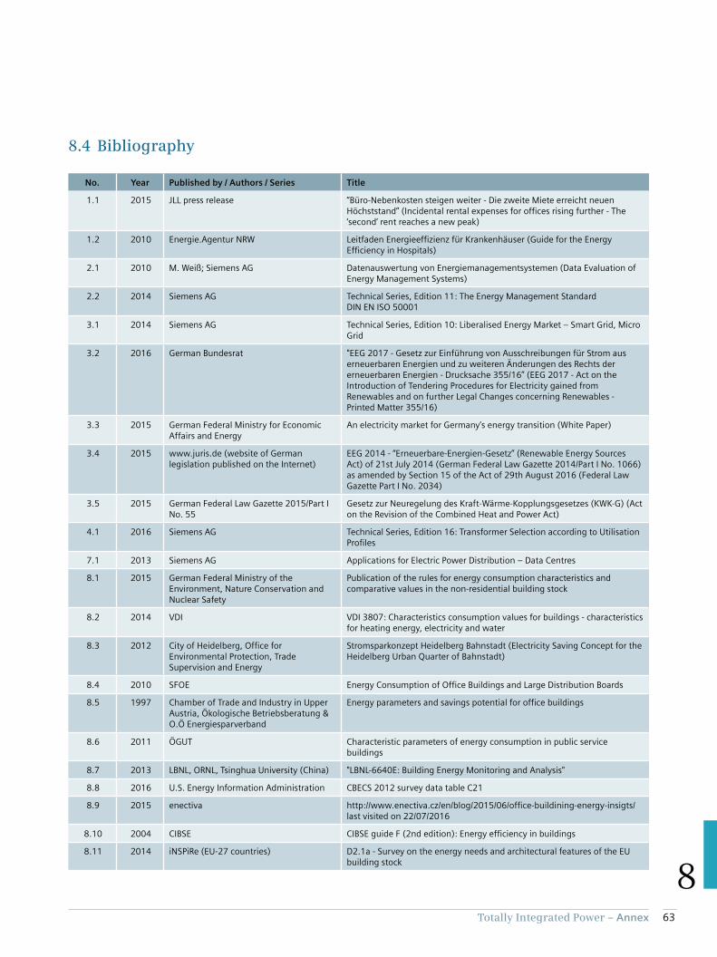
63Totally Integrated Power – Annex
8
8.4 Bibliography
No. Year Published by / Authors / Series Title
1.1 2015 JLL press release “Büro-Nebenkosten steigen weiter - Die zweite Miete erreicht neuen Höchststand” (Incidental rental expenses for offices rising further - The ‘second’ rent reaches a new peak)
1.2 2010 Energie.Agentur NRW Leitfaden Energieeffizienz für Krankenhäuser (Guide for the Energy Efficiency in Hospitals)
2.1 2010 M. Weiß; Siemens AG Datenauswertung von Energiemanagementsystemen (Data Evaluation of Energy Management Systems)
2.2 2014 Siemens AG Technical Series, Edition 11: The Energy Management Standard DIN EN ISO 50001
3.1 2014 Siemens AG Technical Series, Edition 10: Liberalised Energy Market – Smart Grid, Micro Grid
3.2 2016 German Bundesrat "EEG 2017 - Gesetz zur Einführung von Ausschreibungen für Strom aus erneuerbaren Energien und zu weiteren Änderungen des Rechts der erneuerbaren Energien - Drucksache 355/16” (EEG 2017 - Act on the Introduction of Tendering Procedures for Electricity gained from Renewables and on further Legal Changes concerning Renewables - Printed Matter 355/16)
3.3 2015 German Federal Ministry for Economic Affairs and Energy
An electricity market for Germany’s energy transition (White Paper)
3.4 2015 www.juris.de (website of German legislation published on the Internet)
EEG 2014 - “Erneuerbare-Energien-Gesetz” (Renewable Energy Sources Act) of 21st July 2014 (German Federal Law Gazette 2014/Part I No. 1066) as amended by Section 15 of the Act of 29th August 2016 (Federal Law Gazette Part I No. 2034)
3.5 2015 German Federal Law Gazette 2015/Part I No. 55
Gesetz zur Neuregelung des Kraft-Wärme-Kopplungsgesetzes (KWK-G) (Act on the Revision of the Combined Heat and Power Act)
4.1 2016 Siemens AG Technical Series, Edition 16: Transformer Selection according to Utilisation Profiles
7.1 2013 Siemens AG Applications for Electric Power Distribution – Data Centres
8.1 2015 German Federal Ministry of the Environment, Nature Conservation and Nuclear Safety
Publication of the rules for energy consumption characteristics and comparative values in the non-residential building stock
8.2 2014 VDI VDI 3807: Characteristics consumption values for buildings - characteristics for heating energy, electricity and water
8.3 2012 City of Heidelberg, Office for Environmental Protection, Trade Supervision and Energy
Stromsparkonzept Heidelberg Bahnstadt (Electricity Saving Concept for the Heidelberg Urban Quarter of Bahnstadt)
8.4 2010 SFOE Energy Consumption of Office Buildings and Large Distribution Boards
8.5 1997 Chamber of Trade and Industry in Upper Austria, Ökologische Betriebsberatung & O.Ö Energiesparverband
Energy parameters and savings potential for office buildings
8.6 2011 ÖGUT Characteristic parameters of energy consumption in public service buildings
8.7 2013 LBNL, ORNL, Tsinghua University (China) "LBNL-6640E: Building Energy Monitoring and Analysis"
8.8 2016 U.S. Energy Information Administration CBECS 2012 survey data table C21
8.9 2015 enectiva http://www.enectiva.cz/en/blog/2015/06/office-buildining-energy-insigts/ last visited on 22/07/2016
8.10 2004 CIBSE CIBSE guide F (2nd edition): Energy efficiency in buildings
8.11 2014 iNSPiRe (EU-27 countries) D2.1a - Survey on the energy needs and architectural features of the EU building stock
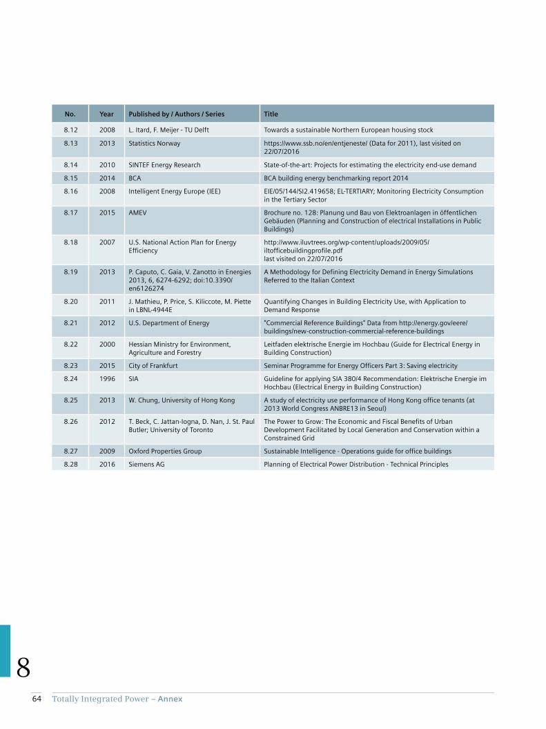
64 Totally Integrated Power – Annex
8
No. Year Published by / Authors / Series Title
8.12 2008 L. Itard, F. Meijer - TU Delft Towards a sustainable Northern European housing stock
8.13 2013 Statistics Norway https://www.ssb.no/en/entjeneste/ (Data for 2011), last visited on 22/07/2016
8.14 2010 SINTEF Energy Research State-of-the-art: Projects for estimating the electricity end-use demand
8.15 2014 BCA BCA building energy benchmarking report 2014
8.16 2008 Intelligent Energy Europe (IEE) EIE/05/144/SI2.419658; EL-TERTIARY; Monitoring Electricity Consumption in the Tertiary Sector
8.17 2015 AMEV Brochure no. 128: Planung und Bau von Elektroanlagen in öffentlichen Gebäuden (Planning and Construction of electrical Installations in Public Buildings)
8.18 2007 U.S. National Action Plan for Energy Efficiency
http://www.iluvtrees.org/wp-content/uploads/2009/05/iltofficebuildingprofile.pdf last visited on 22/07/2016
8.19 2013 P. Caputo, C. Gaia, V. Zanotto in Energies 2013, 6, 6274-6292; doi:10.3390/en6126274
A Methodology for Defining Electricity Demand in Energy Simulations Referred to the Italian Context
8.20 2011 J. Mathieu, P. Price, S. Kiliccote, M. Piette in LBNL-4944E
Quantifying Changes in Building Electricity Use, with Application to Demand Response
8.21 2012 U.S. Department of Energy "Commercial Reference Buildings" Data from http://energy.gov/eere/buildings/new-construction-commercial-reference-buildings
8.22 2000 Hessian Ministry for Environment, Agriculture and Forestry
Leitfaden elektrische Energie im Hochbau (Guide for Electrical Energy in Building Construction)
8.23 2015 City of Frankfurt Seminar Programme for Energy Officers Part 3: Saving electricity
8.24 1996 SIA Guideline for applying SIA 380/4 Recommendation: Elektrische Energie im Hochbau (Electrical Energy in Building Construction)
8.25 2013 W. Chung, University of Hong Kong A study of electricity use performance of Hong Kong office tenants (at 2013 World Congress ANBRE13 in Seoul)
8.26 2012 T. Beck, C. Jattan-Iogna, D. Nan, J. St. Paul Butler; University of Toronto
The Power to Grow: The Economic and Fiscal Benefits of Urban Development Facilitated by Local Generation and Conservation within a Constrained Grid
8.27 2009 Oxford Properties Group Sustainable Intelligence - Operations guide for office buildings
8.28 2016 Siemens AG Planning of Electrical Power Distribution - Technical Principles


Siemens AG Energy Management Medium Voltage & Systems
Mozartstr. 31 c
91052 Erlangen, Germany
For more information, visit
siemens.com/tip-cs
Subject to change without prior notice.
The information in this document only includes
general descriptions and/or performance
characteristics, which do not always apply in the
form described in a specific application, or
which may change as products are developed.
The required performance characteristics are
only binding if they are expressly agreed at the
point of conclusion of the contract.
SENTRON®, SIMATIC® and SIVACON® are
registered trademarks of Siemens AG. Their
unauthorized use is not permissible. All other
brand names in this publication may be trade-
marks, the use of which by third persons for
their own purposes may infringe the rights of
their registered owners.
© Siemens AG 2017
Recommended