FIBER BRAGG GRATING DYNAMIC PRESSURE TRANSDUCER
KEE LI VOON
B. ENG (HONS.) MECHANICAL ENGINEERING
UNIVERSITI MALAYSIA PAHANG
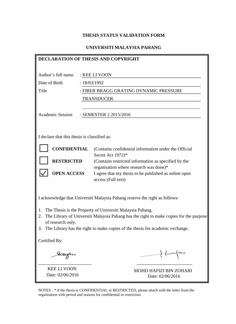
THESIS STATUS VALIDATION FORM
UNIVERSITI MALAYSIA PAHANG
DECLARATION OF THESIS AND COPYRIGHT
Author’s full name : KEE LI VOON
Date of Birth : 18/03/1992
Title : FIBER BRAGG GRATING DYNAMIC PRESSURE
TRANSDUCER
___________________________________________________
Academic Session : SEMESTER 2 2015/2016
I declare that this thesis is classified as:
CONFIDENTIAL (Contains confidential information under the Official
Secret Act 1972)*
RESTRICTED (Contains restricted information as specified by the
organisation where research was done)*
OPEN ACCESS I agree that my thesis to be published as online open
access (Full text)
I acknowledge that Universiti Malaysia Pahang reserve the right as follows:
1. The Thesis is the Property of Universiti Malaysia Pahang.
2. The Library of Universiti Malaysia Pahang has the right to make copies for the purpose
of research only.
3. The Library has the right to make copies of the thesis for academic exchange.
Certified By:
_______________________ ________________________
KEE LI VOON
Date: 02/06/2016
NOTES : * if the thesis is CONFIDENTIAL or RESTRICTED, please attach with the letter from the
organisation with period and reasons for confidential or restriction.
MOHD HAFIZI BIN ZOHARI
Date: 02/06/2016

i
FIBER BRAGG GRATING DYNAMIC PRESSURE TRANSDUCER
KEE LI VOON
Report submitted in partial fulfilment of the requirements
for the award of B. ENG (HONS.) MECHANICAL ENGINEERING
Faculty of Mechanical Engineering
UNIVERSITI MALAYSIA PAHANG
JUNE 2016

ii
SUPERVISOR’S DECLARATION
I hereby declare that I have checked this thesis and in my opinion this thesis is satisfactory
in terms of scope and quality for the award of the degree of Bachelor of Mechanical
Engineering.
Signature:
Name of Supervisor: DR MOHD HAFIZI BIN ZOHARI
Position: LECTURER
Date: 2 JUNE 2016

iii
STUDENT’S DECLARATION
I hereby declare that the work in this thesis is my own except as cited in the references. The
thesis has not been accepted for any degree and is not concurrently submitted in
candidature for any other degree.
Signature:
Name: KEE LI VOON
ID Number: MG12026
Date: 2 JUNE 2016

iv
ACKNOWLEDGEMENT
I would like to use this golden opportunity to express my sincere gratitude and
appreciation to my project supervisor Dr. MOHD HAFIZI BIN ZOHARI for his germinal
ideas, valuable advice, continuous encouragement and constant support throughout this
project. It would be impossible to complete this project successfully without his precious
guidance.
Besides, I am also indebted to University Malaysia Pahang (UMP) for providing the
facilities to carry out my project. Laboratory of UMP also provides a good condition of
equipment and material for me to achieve the completion of the project.
Not to forget, I am grateful to my friends Kek Boon Tat, Lim Lei Kun, Wong Pei
Ing, Irene Kong Che Ling, Goh Xue Mei, Jolie Jong Wan Jia, Chung Kar Yee with their
help and supports they have given to make this study possible.
Last but not least, I acknowledge my sincere indebtedness and gratitude to my
parents for their love, dream and sacrifice throughout my life.

v
ABSTRACT
In this work, a diaphragm type of fiber Bragg grating dynamic pressure transducer
is designed and developed. Before proceeding with a fabrication of the transducer,
simulation software, Autodesks Mechanical Simulation is used to validate the design. The
proposed design of the pressure transducer has a thin metal diaphragm acted as a primary
sensing element and integrated with an FBG sensor acts as a secondary sensing element.
Experiments are conducted to study the static and dynamic response of the FBG sensor. An
air compressor is used to pressurize a test rig and caused in a diaphragm deflection. The
FBG sensor detected applied inner pressure indirectly as the sensor is being stretched or
compressed along its length during the deformation of the diaphragm under different
pressure. A variation in Bragg wavelength of the reflected spectra is observed by using an
Optical Spectrum Analyzer (OSA). A matched edge FBG interrogation system is later
replaced OSA to produce an electrical signal output. Through a reliability test of the FBG
pressure transducer, it is proven to be suitable for pressure measurement for gas or liquid.
The experimental results indicated the FBG sensor has a pressure sensitivity of106 pm/bar.
In addition, the FBG sensor also has an excellent linearity with a fitting linear correlation
coefficient of 99.91% in pressure measurement. From the repeatability test, an error is
found to be less than 0.3%.
vi
ABSTRAK
Dalam kajian ini, satu fiber Bragg grating (FBG) tekanan dinamik transduser yang
berjenis diafragma direka dan dihasilkan. Sebelum meneruskan dengan satu rekaan
transduser, Autodesks Mechanical simulasi, perisian simulasi digunakan untuk
mengesahkan reka bentuk. Reka bentuk tekanan transduser yang dicadangkan mempunyai
satu diafragma dibuat daripada logam yang nipis. Diafragma bertindak sebagai elemen
penderiaan pertama dan bersepadu dengan penderia FBG sebagai elemen penderiaan kedua.
Eksperimen dijalankan untuk mengkaji tindak balas statik dan dinamik penderia FBG itu.
Pemampat udara digunakan untuk memberi tekanan kepada pelantar ujian dan
menyebabkan defleksi diafragma. Penderia FBG mengesankan tekanan dalaman secara
tidak langsung apabila penderia sedang diregangkan atau dimampatkan sepanjang
panjangnya semasa diafragma berubah bentuk di bawah tekanan yang berbeza.
Kepelbagaian dalam Bragg panjang gelombang spektrum diperhatikan dengan
menggunakan satu penganalisis optikal spektrum (OSA). Satu sistem perekod data yang
berasaskan FBG penuras sepadan kemudiannya menggantikan OSA untuk menghasilkan
isyarat elektrik dengan menambah satu lagi FBG sebagai penapis. Melalui ujian
kebolehpercayaan FBG tekanan transducer, ia terbukti sesuai untuk pengukuran tekanan
untuk gas atau cecair. Keputusan eksperimen menunjukkan sensor FBG mempunyai
kepekaan tekanan sebanyak 106 pm / bar. Di samping itu, penderia FBG juga mempunyai
kelinearan yang baik dengan pekali korelasi linear pemasangan 99.91% dalam pengukuran
tekanan. Dari ujian kebolehulangan, ralat didapati tidak kurang daripada 0.3%

vii
TABLE OF CONTENTS
Page
SUPERVISOR’S DECLARATION ii
STUDENT’S DECLARATION iii
ACKNOWLEDGEMENTS iv
ABSTRACT v
ABSTRAK vi
TABLE OF CONTENTS vii
LIST OF TABLES xi
LIST OF FIGURES xii
LIST OF ABBREVIATIONS xv
CHAPTER 1 INTRODUCTION
1.1 Introduction 1
1.2 Project Background 1
1.3 Problem Statement 2
1.4 Objectives 2
1.5 Scope 3
1.6 Project Planning 3
1.7 Thesis Hypothesis 3
1.8 Impact, Significance and Distribution 3
1.9 Outline of Report 4
CHAPTER 2 LITERATURE REVIEW
2.1 Introduction 5
2.2 History of Pressure Measurement 5

viii
2.2.1 Pressure and Its Unit of Measurement 7
2.3 Static and Dynamic Pressure 7
2.3.1 Pitot Tube 9
2.4 Types of Pressure 10
2.4.1 Absolute Pressure 11
2.4.2 Gauge Pressure and Vacuum 11
2.4.3 Differential Pressure 12
2.5 Pressure Transducer 12
2.5.1 Measuring Methods of Pressure 12
2.5.1 Types of Pressure Transducer 14
2.6 Pressure Sensing Element 14
2.7 Fiber Bragg Grating Sensing Technology 15
2.8 Fiber Bragg Grating Dynamic Pressure Sensing Process 16
2.8.1 Sensing Principle of FBG 16
2.9 Fiber Bragg Grating Dynamic Sensing System 19
2.9.1 Interrogation System 19
2.10 Diaphragm Design 30
2.10.1 Working Principle of Diaphragm 30
2.10.2 Effect of Diaphragm Geometry on Pressure Sensor’s
Performance
31
2.11 Types of Deformation of the FBG with a.Diaphragm-Type Pressure
Transducer
32
2.12 Chapter Conclusion 34
CHAPTER 3 METHODOLOGY
3.1 Introduction 36
3.2 Project flow chart 36
3.3 Concept Design 38
3.3.1 Simulation Analysis 39

ix
3.4 Fabrication Process 42
3.5 Interrogation System 48
3.6 Experimental Setup 49
3.7.1 Calibration 49
3.7.2 Pipe Leak Test 53
3.7 Chapter Conclusion 54
CHAPTER 4 RESULTS AND DISCUSSION
4.1 Introduction 55
4.2 Results 55
4.2.1 Optical Signal 55
4.2.2 Electrical Signal 58
4.3 Dynamic Response during a Leakage 65
4.4 Data Validation with Pressure Gauge 66
4.5 Effect of Amplification of the Photodetector 69
4.6 Simulation Results of the Pressure Transducer 69
4.7 Normalized Output Signal 70
4.8 Chapter Conclusion 75
CHAPTER 5 CONCLUSION AND RECOMMENDATION
5.1 Introduction 76
5.2 Conclusion of Study 76
5.3 Problems 77
5.3 Recommendation 77
5.4 Future Works 78
5.4.1 Analysis on the Mechanical Part 78
5.4.2 Temperature Compensation of FBG Pressure Transducer 79
5.4.3 A Comparison between FBG Sensor and Other Electronic 79

x
Sensors
REFERENCES 80
APPENDICES
A Gantt Chart 86
B Solidwork Drawing 87
C Matlab Coding 91
D Setup Sheet for CNC Machine 98
E G Code for CNC Machine 106
F List of Material and Equipment 115
G Matlab Coding for Normalization of Voltage 118
H Matlab GUIDE 126

xi
LIST OF TABLES
Table No. Page
3.1 Specification of Diaphragm 40
4.1 Summarized Data of Comparison between Pressure Gauge and FBG
Sensor
68
4.2 Factor of Safety (FOS) of Diaphragm 70
4.3 Calibration Curve on Different Days 72
4.4 Summarized Data of Comparison between Pressure Gauge and FBG
Sensor after Normalizing the Voltage
74

xii
LIST OF FIGURES
Figure No. Page
2.1 Pitot Tube Measurement 9
2.2 Pitot- Darcy Probe is Used for Both Static and Dynamic
Measurement
10
2.3 Pressure Types based on Different Reference Points 12
2.4 Schematic of Elastic Pressure Transducers 13
2.5 Transmission and Reflection Spectra from an FBG 17
2.6 Data Path of FSIM 20
2.7 Schematic Diagram of FSRMI 21
2.8 FBG Interrogation Method by Using a Demodulator 21
2.9 Matched Edge Filter Arrangement for Dynamic Sensing 22
2.10 Schematic Diagram of the Movement of Light in the Circulator-based
System
22
2.11 The Resultant of Optical Signal through a FBG Filter in Matched
Edge Filter Method
23
2.12 A Schematic Diagram of Mismatched Edge Filter 24
2.13 Principle of Operation of a Linear Edge Filter Utilizing an Optically
Mismatched FBG
25
xiii
2.14 Principle of Operation for a Detection System Using a Tunable Laser
Source
26
2.15 An Experimental Setup for Comparison of Two Systems in
Ultrawave Detection
26
2.16 Structure of High Speed FBG Interrogation System 28
2.17 Fast FBG Interrogation 29
2.18 FBG Dynamic Strain Measurement 29
2.19 Circular Diaphragm and Its Strain Distribution Curve 31
2.20 Coordinates and Displacements of Elliptical Plate 32
2.21 Structure Diagram of Flat Diaphragm FBG Pressure Sensor with
Longitudinal Deformation
33
2.22 Structure Diagram of Flat Diagram FBG Pressure Sensor with L-
shaped Lever
34
2.23 Structure Diagram of Flat Diagram of FBG Pressure Sensor with
Lateral Deformation
34
3.1 Project Flow Chart 36
3.2 Concept Design of Transducer 39
3.3 Meshing of the Diaphragm 40
3.4 Displacement Analysis of the Diaphragm 40
3.5 Factor of Safety Analysis of the Diaphragm 41
3.6 Von Mises Stress Analysis of the Diaphragm 41

xiv
3.7 Lathe Machine 42
3.8 Machining in Process 42
3.9 Lathed Products,(a)Base and (b) Diaphragm 43
3.10 CNC Milling Machine 43
3.11 Drawing in Mastercam X5 (a) Base and (b) Diaphragm 44
3.12 (a) and (b) Types of Tools Used 45
3.13 Calibration of Tool on Z-axis 45
3.14 CNC Finished Products (a) Diaphragm and (b) Base 46
3.15 Assembly of the Pressure Transducer 46
3.16 3D Printed Cover 47
3.17 FBG Dynamic Pressure Transducer 47
3.18 Matched Edge Interrogation System 48
3.19 Air Compressor 50
3.20 Calibration Test Rig 50
3.21 National Instruments Setup for FBG Sensor 51
3.22 Overview of Dasylab Work Layout 51
3.23 Overall Experimental Setup 52
3.24 Matlab’s GUI 53
3.25 Pipe Leak Detection Test Rig 54

xv
4.1 OSA Output in Sense2020 56
4.2 The Spectra of Bragg Wavelength Shift of the Sensing FBG at
Different Applied Pressure Values from 0 Until 5 bar, Respectively
57
4.3 Variation of Wavelength of FBG versus Pressure 57
4.4 Variation of Wavelength Shift Difference of FBG versus Pressure 58
4.5 Output Voltage of the Sensor from 0 to 5 bar 59
4.6 Wavelength Variation from (a) 0 bar, (b) 1 bar and (c) 2 bar 60
4.7 Wavelength Variation at 3 bar 62
4.8 Wavelength Variation from (a) 4 bar and (b) 5 bar 63
4.9 FBG Sensor Calibration Graph and Linear Regression 64
4.10 Repeatability of the Transducer 65
4.11 Dynamic Response of FBG Sensor during a Pipe Leakage 66
4.12 Structure of a C-Shaped Bourdon Tube Pressure Gauge 67
4.13 Data Validation with Pressure Gauge 68
4.14 Daily Calibration Record 71
4.15 Normalized Voltage against Pressure 72
4.16 Modified Matlab GUI 73
4.17 Data Validation with Pressure Gauge after Normalizing the Voltage 74

xvi
LIST OF ABBREVIATIONS
FBG Fiber Bragg Grating
mm millimeter
V volts
kPa kilopascal
ms millisecond
% percent
dB decibel
OSA Optical Spectrum Analyzer
ASE Amplified Spontaneous Emission
SLED Super Luminescent Diode
CHAPTER 1
INTRODUCTION
1.1 INTRODUCTION
This chapter provides a detailed explanation on project background, problem
statement, project objective and scope. Gantt chart included in this section which explains
the overall procedure and time distribution for this project.
1.2 PROJECT BACKGROUND
In this project, dynamic pressure in the fluid is studied and instrumented with a
dynamic pressure transducer. Currently, there are a plenty amount of transducers available
in the market to provide high-reliability dynamic measurements in high-temperature
environments, some of them can perform in an environment up to +538 degrees Celsius.
They are capable of dynamic and high-frequency pressure measurement and ideal for
monitoring explosion, pulsation pressure, fast pressure variations, surges and dynamic blast
(Walter, 2004). In another way, dynamic pressure sensors can also serve as acoustic
sensors. Therefore, it is suitable for a broad range of applications such as propulsion testing
in aerospace, explosive component testing (e.g. detonator, explosive bolts), monitoring of
combustor instability in combustion studies, airbag and anti-lock braking systems (ABS)
testing in automotive and measurement of air blast shock waves.
2
There are many ways to detect or sense the dynamic response of a fluid pressure. In
this project, a robust and practical transducer in dynamic pressure sensing is being designed
and developed and investigated the pressure sensitivity.
1.3 PROBLEM STATEMENT
The conventional dynamic pressure transducer is using a metal foil strain gauge to
detect the pressure change in fluid flow. It can be used to detect a subtle distortion by the
elastic deformation element, a thin aluminium diaphragm in the transducer. However, there
are some drawbacks when using a strain gauge for dynamic pressure sensing.
It has some disadvantages when it comes to detecting the dynamic response of pressure
in a harsh environment due to large size, limited temperature range, and low sensitivity.
This sensing element is very sensible to temperature and electromagnetic field which affect
the sensitivity (Edwards, 2000). Besides that, strain gauge has a difficulty when bonds it to
the diaphragm by adhesive, an imperfect bonding between the sensor and the structure will
result in poor dynamic pressure sensing with significant effects(Zohari, 2014). Furthermore,
dynamic pressure sensing is unable being monitored from long distance by using a strain
gauge because it is not capable of transmitting data over long distances with little or
no loss in signal integrity.
1.4 OBJECTIVE
a. To design and develop a Fiber Bragg Grating (FBG) dynamic pressure transducer.
b. To investigate the sensitivity of the dynamic pressure transducer.

3
1.5 SCOPE
a. An FBG sensor with a center wavelength of 1546.97nm with a peak reflectivity of
99.91%.
b. Matched edge filter interrogation method used for demodulation of the signal.
c. An FBG sensor installed at the pressure transducer on a diaphragm using an epoxy
glue to sense the deformation.
d. Temperature effect towards the sensitivity is not investigated in this project as both
sensors perform at room temperature.
1.6 PROJECT PLANNING
The whole plan for the project shown in both Gantt chart for Semester I and
Semester II as attached in Appendix A.
(Refer to Appendix A)
1.7 THESIS HYPOTHESIS
The deployment of FBG sensor into the pressure transducer is suitable to detect
both static and dynamic pressure.
1.8 IMPACT, SIGNIFICANCE AND CONTRIBUTION
The installation the FBG sensors easier compared to the strain gauge into the
diaphragm-type dynamic pressure transducer. Installing a large number of conventional
electrical strain gauges is time-consuming and needed to be handled with care as its
performance is dependent on the bond between itself and the test part.
Before the installation, proper preparation of the surface to ensure the strain gauge
is bonded to the surface correctly. The aim of surface preparation is to develop a chemically

4
clean surface having a roughness appropriate to gauge installation requirement. The steps
involved in the surface preparation are solvent degreasing, surface abrading, application of
gauge layout lines, surface conditioning and neutralizing. And there are many steps during
the installation to position the strain gauge at the right place and apply adhesive to bond the
strain gauge onto the diaphragm surface. After the installation, soldering has to be carried
out between gauge and its associated bond pad. Bond pads are then connected by electrical
wires by soldering and routed to the data acquisition system(Nichols, 1970).
By comparison, the diaphragm can be instrumented by FBG sensors easily by
bonding an optical fiber and connecting them to single FBG circulator, and the dynamic
pressure transducer is ready to be calibrated and used in dynamic sensing. This installation
is straightforward and quick so that it can save cost and time. In short, FBG sensor has a
great potential to enhance user satisfactory in measurement and instrumentation and able to
detect and actuate the dynamic pressure in all types of industry.
1.9 OUTLINE OF REPORT
This report consists of five chapters. The first chapter describes the background,
problem statement, objectives, and scope of the project. The second chapter discusses the
theory and literature reviews that which have been done. The third chapter describes the
methodology approach of this project. The fourth chapter discusses the result and
discussion based on the output of this system. The last chapter describes the conclusion of
the project and suggestion of future work that can be done to improve this project.
CHAPTER 2
LITERATURE REVIEW
2.1 INTRODUCTION
This chapter further discusses in detailed about the history of the pressure
measurement, brief introduction about static and dynamic pressure, types of pressure
measurement, measuring elements, fiber Bragg grating (FBG) sensor and interrogation
system and lastly diaphragm design.
2.2 HISTORY OF PRESSURE MEASUREMENT
Pressure measurement began from the middle of the seventeenth century with the
discovery of using a glass tube filled with mercury can measure the atmospheric pressure
by Evangelisti Torricelli(Kizz, 2008), a student to Galileo Galilei(Hilliam, 2005). In 1594,
Galileo found that the limit for water to rise in the suction pump was only 10m, and the
reason remained unknown(Stein, 2013). In 1644, Torricelli was driven by this question and
brought some scientific investigations. Blaise Pascal named the force he found which keeps
the column at 760mm as “pressure” exerted by the weight of air above the
column(Applebaum, 2003). He also stated that the pressure is distributed uniformly in all
directions.

6
During the Industrial Revolution, a variety of pressure measurement methods were
introduced and applied in the steam power plant and began the development of the science
of thermodynamics(Achuthan, 2009). Mechanical measurement technology in 1843-1849:
aneroid barometer and bourdon tube pressure gauge created by Lucien Vidie and Eugene
Bourdon(Baukal Jr, 2012). After 1930, there comes an electrical measurement technology
which utilized transduction mechanism from the movement of the diaphragm, Bourdon
tube, and spring then converted them into electrical quantity by the capacitance(Tang,
2006). The strain gauge first developed in 1938 by E.E. Simmons of the California Institute
of Technology and AC. Ruge of Massachuseffs Institute of Technology(Busch-Vishniac,
2012). Enhancing the performance, strain gauge integrated with a full resistor bridge.
However, the bonding connection between gauge and diaphragm caused hysteresis and
instability.
A thin-film transducer was announced to provide excellent stability and low
hysteresis by Statham. Therefore, it is suitable for high-pressure measurement(Kubba &
Jiang, 2014). In the modern era, it is still widely used for the high-pressure measurement.
William R. Poyle invented capacitive transducers on glass and quartz basis and applied a
patent for it in 1973, and few years later, Bob Bell of Kavlico modified it with a ceramic
basis to suit for lower pressure range which thin-film was not suitable for this range(Asundi,
2011).
In this modern era, new technologies like piezoelectric, capacitance,
electromagnetic and optical based pressure transducers are available to be deployed in
different applications. Pressure measurement is an essential element in most of the
manufacturing process and laboratory testing because the accuracy of the measurement has
a significant effect on the validity of result, product quality, energy efficiency and safe
operation of a process(Tilford, 1992).
7
2.2.1 PRESSURE AND ITS UNIT OF MEASUREMENT
Pressure is a normal force exerted by a fluid per unit area which force exerted by
gasses or vapors, liquids, and solid bodies (von Beckerath, 1998; Yunus & Cimbala, 2006).
In metric unit (SI), force is expressed in a unit of Newton (N) and Pascal (Pa) for pressure
as in Eq. (2.1).
(2.1)
There are two types of pressure which are static and dynamic pressure.
2.3 STATIC AND DYNAMIC PRESSURE
For static pressure, the fluid is immovable, and the pressure is exerted uniformly to
the fluid in all directions. Thus, the static pressure is independent of direction no matter
which direction the fluid flows. Unlike dynamic pressure, it only exists in the fluid in
motion and acts as a directional component of fluid pressure. In a fluid system,
measurement of velocity and pressure based on dynamic pressure can be used as a
diagnostic for determining various quantities. On the other hand, loads exerted on the pipe
walls is measured by static pressure(Goldstein, 1996).
The Bernoulli equation states that the sum of the flow, kinetic, and potential
energies of a fluid particle along a streamline is constant(Batchelor, 2000). The pressure
change can be caused by the energy conversion from kinetic and potential energy to flow
energy (and vice versa) during flow. Bernoulli equation is multiplied by density give a
clearer explanation of this phenomenon(Yunus & Cimbala, 2006) as in Eq.(2.2).
8
P is the static pressure, and it does not incorporate any dynamic effect. It states the
actual thermodynamic pressure of the fluid.
, is a dynamic pressure that represents the
pressure rise when the fluid in motion is brought to stop isentropically. The last term,
is the hydrostatic pressure term, its value depends on the reference level selected, and it
accounts for the elevation effects such as fluid weight on pressure.
The total pressure of the flow is the sum of these three types of pressure and
measured by a measuring instrument which is facing the same direction with the flow.
According to Bernoulli equation (Munson, Young, & Okiishi, 1990; Shames & Shames,
1982; Shaughnessy, 2010; Yunus & Cimbala, 2006), total pressure along a streamline is
constant. Stagnation pressure exists at a point where the fluid is brought to a complete stop
isentropically, and it is a sum of static and dynamic pressure. Thus, dynamic pressure also
can be described as in Eq. (2.3).
(2.3)
From the equation above, dynamic pressure is a difference between stagnation
pressure and static pressure. Therefore, it is a differential pressure rather than gauge or
absolute because it is referred to the static pressure in the fluid system and not atmospheric
pressure. Pitot tube is a measuring instrument for dynamic pressure.

9
2.3.2 PITOT TUBE
Figure 2.1: Pitot Tube Measurement (Yunus & Cimbala, 2006).
Traditionally, determination of the dynamic pressure and fluid velocity can be done
by using Pitot tube and a static pressure tap where Pitot tube provides stagnation pressure
and the latter one measures static pressure. For example, Pitot tube is widely used in
airplane unit to measure the air speed and flow rate during the flight. However, this
measurement device needs to be connected to pressure measurement devices such as a U-
tube manometer or a pressure transducer(Yunus & Cimbala, 2006). A more convenient
design is innovated to integrate static pressure holes on a Pitot probe, Pitot-static probe
(also called a Pitot-Darcy probe) then connected to a pressure transducer or a manometer
measures the dynamic pressure and solves the fluid velocity directly("Pitot-static tube,"
1927).
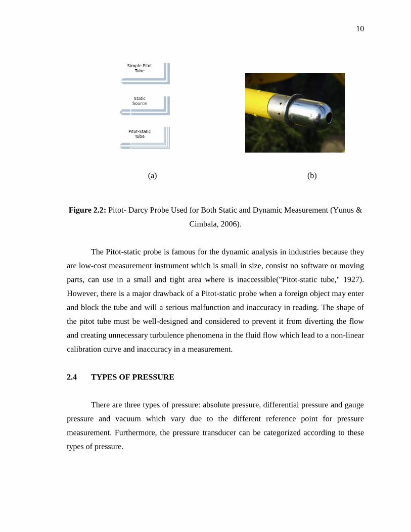
10
(a) (b)
Figure 2.2: Pitot- Darcy Probe Used for Both Static and Dynamic Measurement (Yunus &
Cimbala, 2006).
The Pitot-static probe is famous for the dynamic analysis in industries because they
are low-cost measurement instrument which is small in size, consist no software or moving
parts, can use in a small and tight area where is inaccessible("Pitot-static tube," 1927).
However, there is a major drawback of a Pitot-static probe when a foreign object may enter
and block the tube and will a serious malfunction and inaccuracy in reading. The shape of
the pitot tube must be well-designed and considered to prevent it from diverting the flow
and creating unnecessary turbulence phenomena in the fluid flow which lead to a non-linear
calibration curve and inaccuracy in a measurement.
2.4 TYPES OF PRESSURE
There are three types of pressure: absolute pressure, differential pressure and gauge
pressure and vacuum which vary due to the different reference point for pressure
measurement. Furthermore, the pressure transducer can be categorized according to these
types of pressure.

11
2.4.1 ABSOLUTE PRESSURE
It represents the pressure difference between the point of measurement and a perfect
vacuum where pressure is zero(von Beckerath, 1998). It is equal to a sum of gauge pressure
with atmospheric pressure. Atmospheric pressure is the weight exerted by the overhead
atmosphere on a unit area of surface and mean atmospheric pressure at sea level is given
equivalently as P = 1.013x10⁵ Pa = 1013 hPa = 1013 mb = 1 atm = 760 torr(Yunus &
Cimbala, 2006). As the altitude increases, the atmospheric pressure decreases until it
practically becomes zero (full vacuum) and also influenced by climate changes as shown by
the daily weather report(von Beckerath, 1998).
2.4.2 GAUGE PRESSURE AND VACUUM
It is a pressure difference between the measured pressure at a point and the
atmospheric pressure(Yunus & Cimbala, 2006). This pressure type is the standard
measurement, and the only pressure difference is concerned regardless variation of
atmospheric pressure in different altitudes and climates. The pressure measured below
atmospheric pressure is called vacuum pressure.
12
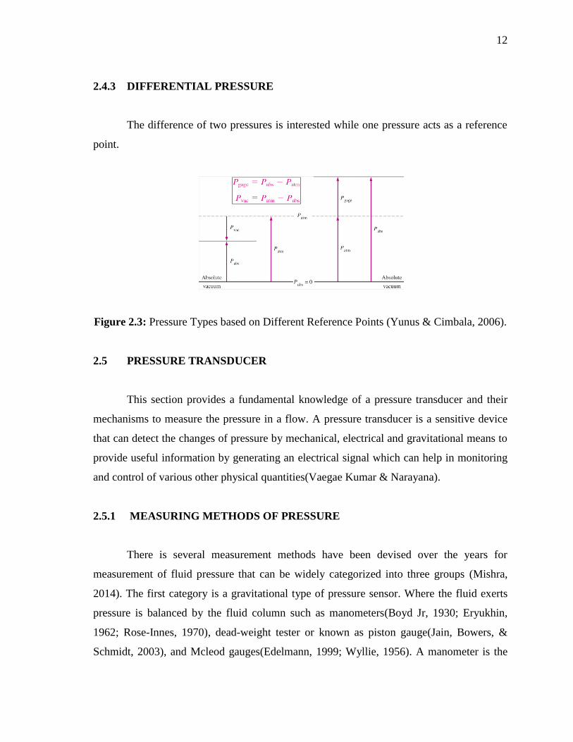
2.4.3 DIFFERENTIAL PRESSURE
The difference of two pressures is interested while one pressure acts as a reference
point.
Figure 2.3: Pressure Types based on Different Reference Points (Yunus & Cimbala, 2006).
2.5 PRESSURE TRANSDUCER
This section provides a fundamental knowledge of a pressure transducer and their
mechanisms to measure the pressure in a flow. A pressure transducer is a sensitive device
that can detect the changes of pressure by mechanical, electrical and gravitational means to
provide useful information by generating an electrical signal which can help in monitoring
and control of various other physical quantities(Vaegae Kumar & Narayana).
2.5.1 MEASURING METHODS OF PRESSURE
There is several measurement methods have been devised over the years for
measurement of fluid pressure that can be widely categorized into three groups (Mishra,
2014). The first category is a gravitational type of pressure sensor. Where the fluid exerts
pressure is balanced by the fluid column such as manometers(Boyd Jr, 1930; Eryukhin,
1962; Rose-Innes, 1970), dead-weight tester or known as piston gauge(Jain, Bowers, &
Schmidt, 2003), and Mcleod gauges(Edelmann, 1999; Wyllie, 1956). A manometer is the

13
oldest method to measure the fluid pressure. A researcher(Thony & Vachaud, 1980) made
use of the working principle of mercury manometer with an outer face of the glass tubing
covered with a transparent metallic oxide. It acted as the fixed outer electrode of a
capacitor to develop a cost effective, new and reliable pressure transducer by the concept
capacitance which changed linearly with the position of the mercury in the tube.
The following type of sensor is direct acting elastic. The pressure force acting on it
can be used to measure the acting pressure by elastic deformation. For examples, Bourdon
tubes(Balkanli, 1981; Filloux, 1969; Kennedy, 1954; Marick, Bera, & Bera, 2014),
bellows(Cui, Long, & Qin, 2015; Jones & Dunphy, 2006; Vijai Kumar, 1983; Vaegae
Kumar & Narayana), elastic membranes(Mishra, 2014), and diaphragms(Pinet, 2011).
Apart from that, electrical quantities and concepts such as resistance, conductivity,
piezoelectric effects and ionization are applied in the pressure measuring devices in indirect
acting elastic. For examples, strain gauges are the most modern sensor in dynamic pressure
measurement and suitable for narrow-span pressure and differential pressure
measurements(Sharma & Ojha, 2012).
Figure 2.4: Schematic of Elastic Pressure Transducers: (a) Bourdon tube, (b) Diaphragm,
and (c) Bellows(Mishra, 2014).

14
2.5.2 TYPES OF PRESSURE TRANSDUCER
Pressure transducers classified into several categories. If the pressure port exposed
to the atmosphere, it is a gage pressure transducer. When the transducer connected to two
pressures, it is a differential pressure transducer. Absolute pressure transducer has a
pressure port within a sealed vacuum region or at a given pressure. In the proposed design,
it is a gage pressure transducer as a reference point is at atmospheric pressure.
2.6 PRESSURE SENSING ELEMENT
For a transducer, it is a flexible metallic material, and it will deform or expand due
to the pressure which acting on it. A sensor attaches to the elastic material for detection of
the deformation from the transducer to get an accurate measurement. The diaphragm-type
transducer chosen because it provided high accuracy and better dynamic response and had
three shapes which are flat, corrugated or capsule-shaped and fastened to the
housing(Mishra, 2014). Anil Kumar Sharma and Anuj Kumar Ojha(Sharma & Ojha, 2012)
also agreed that diaphragms are more popular due to less space to generate sufficient
deformation or motion for operating electronic transducers.
Most of the pressure transducer are using the flat-diaphragm (Huang, Zhou, Wen, &
Zhang, 2013; Pachava, Kamineni, Madhuvarasu, & Putha, 2014; Vengal Rao,
Srimannarayana, Sai Shankar, Kishore, & Ravi Prasad, 2012). Commonly, the strain gauge
acts as a sensor for diaphragm type- transducer to measure the local strain which able to
indicate the level of applied pressure. Weiguo Lin and Xin Zhang (W. Lin & Zhang, 2006)
proposed a dynamic pressure transducer to detect leak detection of an oil pipeline. This
approach used the characteristic of the piezoelectric sensor. The piezoelectric sensor can
reflect leakage more quickly and sensitively than another absolute pressure transducer.
However, there are some drawbacks of the electronic sensing element. The accuracy of the
sensors will be affected by electromagnetic interference such as lightning event, explosive
environment, and chemical reaction. In an explosive environment, a spark from the
electrical wire of the sensor will initiate a gas explosion which is dangerous. Therefore, a
15
sensor which transmits optical signal which immunes to an electromagnetic field and can
apply in the harsh environment because it offers high safety to replace the electrical sensor.
2.7 FIBER BRAGG GRATING SENSING TECHNOLOGY
The formation of optical fiber reported in 1978 at the Canadian Communications
Research Centre (CRC), Ottawa, Ont., Canada by Hill et al. (K. Hill, Fujii, Johnson, &
Kawasaki, 1978). The fabrication method of the optical fiber is uncontrollable and
ineffective which slow the development of the optical fiber. After the suitable method of
the manufacture of FBG was devised in the year 1989, a more intensive study on fiber
gratings began(Meltz, Morey, & Glenn, 1989). In late 1990’s, the optical fiber is widely
used in the telecommunication industry. Optical fiber sensing technologies available
nowadays is mainly consisting three different types of optical sensing element. There are
intensity-based, fiber Bragg grating (FBG) based and Fabry-Perot cavity based (Bremer et
al., 2014; Chen, 2010; Knute & Bailey, 1992; Pinet, 2011; X. X. Wang & Wu, 2012; Zhu &
Wang, 2005).
Recently, increasing interest in worldwide industries towards the application of
FBG in sensing technology has brought to the rapid development and deployment of optical
sensors especially in the monitoring of temperature and strain. Stephen J.
Mihailov(Mihailov, 2012) has described the fiber Bragg gratings (FBGs) as an optical
filtering sensor that reflects light of a particular wavelength is present within the core of an
optical fiber waveguide.
FBG has many advantages, these include relatively small size and long life span,
significant progress has been made in applications to strain measurement(Shu et al.). It is
also inexpensive to produce, lightweight, multiplexing, self-referencing with a linear
response, ease of installation, durability and immune to electromagnetic interference (EMI)
(Kersey, 1996; Othonos & Kalli, 1999; Yang, Annamdas, Wang, & Zhou, 2008).
Moreover, a pressure quasi-distributed measure can be realized by multiplexing in one
16
single optical fiber to provide multiple FBG sensing element without has to install a huge
number of the strain gauge(Huang et al., 2013).
Sensing process in extremely harsh environments such as explosion gas
environment or high-temperature combustion chamber and environment which contains
high electromagnetic interference is feasible by using FBG sensors due to its passive
nature. Although naked FBG sensor is fragile, an approach to encapsulate the FBG sensor
could solve the problem. By adding carbon fiber for reinforcement and solidified by epoxy
resin with encapsulation technique(Li Liu, CHEN, Zhang, Wu, & Liu, 2012).The
encapsulation technology protects the fiber from the severe environment in mounting
processing without influencing the transmission of the strain applied to the FBG(Shu et al.).
With these advantages, FBGs can use in dynamic pressure measurement.
2.8 FIBER BRAGG GRATING DYNAMIC SENSING PROCESS
2.8.1 SENSING PRINCIPLE OF FBG
FBG sensors are produced by creating periodic variations in the refractive index of
the core of an optical fiber by using a high energy optical source and a phase mask(Meltz
et al., 1989). Fig. 3 shows the internal structure of an FBG sensor. Reflection of particular
wavelength occurs when the light is traveling at the Bragg wavelength, which is a grating
feature and appears missing in the transmission spectrum also shown in the diagram below
when the grating structure only allows wavelengths of light that are not in resonance with it
to pass through it(Mihailov, 2012).

17
Figure 2.5: Transmission and Reflection Spectra from an FBG(Majumder, Gangopadhyay,
Chakraborty, Dasgupta, & Bhattacharya, 2008).
Bragg wavelength is a narrowband spectral output, or a peak reflected wavelength
from the FBG sensor after being illuminated by broadband light source and the light
interacts with the grating of an FBG. The detection of local strain from a deformation has
done through the variation of grating period and the reflected wavelength via the Bragg
equation. According to the Bragg condition, the Bragg wavelength can be expressed in a
well-known formula (Yun-Jiang Rao, 1997) as in Eq. (2.4):
(2.4)
Where is Bragg grating wavelength, is grating periodic spacing, and neff is the
effective reflective index of the fiber core.This formula is established by Nobel Laureate Sir
William Lawrence Bragg in 1915 about diffraction of X-Ray from crystals, and he
expressed it into a simple mathematical formula.
The Bragg wavelength is sensitive to physical changes in the grating due to strain
and temperature(Shu et al.). Thermal expansion in the FBG caused the effective refractive
index and the spacing of the gratings to change simultaneously and produced a wavelength
shift. Over 30 years, the wavelength shift of the FBG has been documented(K. O. Hill &
18
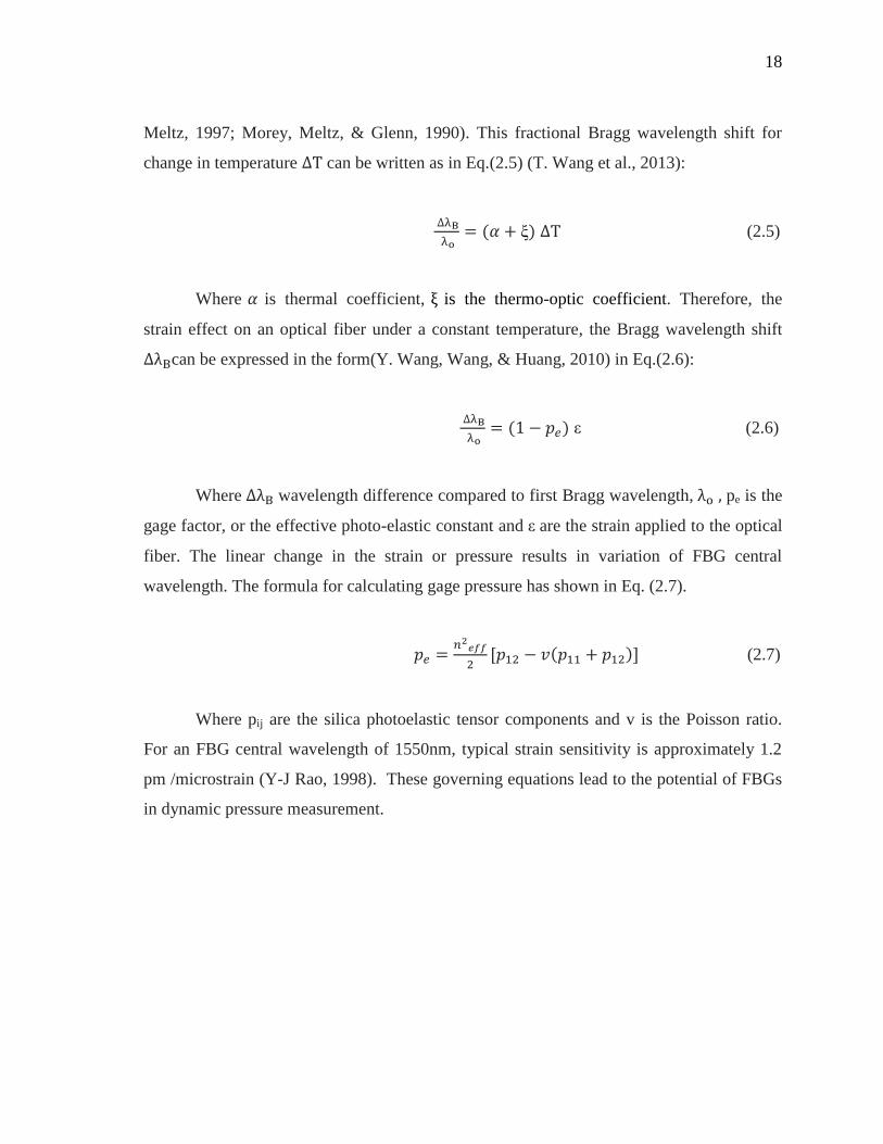
Meltz, 1997; Morey, Meltz, & Glenn, 1990). This fractional Bragg wavelength shift for
change in temperature can be written as in Eq.(2.5) (T. Wang et al., 2013):
(2.5)
Where is thermal coefficient, is the thermo-optic coefficient. Therefore, the
strain effect on an optical fiber under a constant temperature, the Bragg wavelength shift
can be expressed in the form(Y. Wang, Wang, & Huang, 2010) in Eq.(2.6):
(2.6)
Where wavelength difference compared to first Bragg wavelength, pe is the
gage factor, or the effective photo-elastic constant and are the strain applied to the optical
fiber. The linear change in the strain or pressure results in variation of FBG central
wavelength. The formula for calculating gage pressure has shown in Eq. (2.7).
(2.7)
Where pij are the silica photoelastic tensor components and v is the Poisson ratio.
For an FBG central wavelength of 1550nm, typical strain sensitivity is approximately 1.2
pm /microstrain (Y-J Rao, 1998). These governing equations lead to the potential of FBGs
in dynamic pressure measurement.

19
2.9 FIBER BRAGG GRATING DYNAMIC SENSING SYSTEM
When encountered with fluctuation in pressure or variation in pressure that
undergoes changes over time, dynamic pressure measurement system has to be a fast-
responding and high sensitivity to detect even a slight pressure changes. The dynamic
measurement system can use the pressure flow fluctuation to induce a mechanical
oscillatory motion on elastic sensors. Therefore, the motion will be sensed, conditioned,
transmitted and converting the signal to display it in the electrical signal to be further
analyzed the pressure monitoring by data processing in the computer user interface. The
signal output as an electrical signal is desired to be linearly proportional to pressure
obtained in the measurement. An interrogation system for optical sensor has to be
developed to convert the signal.
2.9.1 INTERROGATION METHODS
There are many different interrogation methods (López-Amo & López-Higuera,
2011).Interrogation unit used in the pressure measuring system to read the Bragg
wavelength shift of the FBG caused by deformation of the elastic element like diaphragm
induced pressure exerted on it. Selection of interrogation method based on several factors
such as type and range of strain measured, accuracy and sensitivity required, the number of
sensors interrogated and cost of the instrumentation(Zohari, 2014).
Two types of FBG interrogation schemes are passive and active detection scheme.
For the passive detection system, it includes a linearly wavelength-dependent device(Melle
& Liu, 1992), CCD spectrometer(Kersey et al., 1997), power detection(Grubsky &
Feinberg, 2000) and identical chirped-grating pair(Fallon, Zhang, Gloag, & Bennion,
1997). For active detection system, includes Fabry-Perot filter(Kersey, Berkoff, & Morey,
1993), unbalanced Mach-Zehnder interferometer(Kang, Lee, Choi, & Lee, 1999), fiber
Fourier transform spectrometer(Davis & Kersey, 1995). Other than that, a matched FBG
pair(Kang et al., 1998), Michelson interferometer and LPG pair interferometer(JUNG,
LEE, & LEE, 2000) are also under active detection scheme in FBG interrogation.

20
Commercial interrogators(Verbruggen, 2009; Xiong et al., 2012)in the market
customized for a range of specific applications with different demand in sensing included
the number of sensors, types of multiplexing used and level of precision and resolution but
it is expensive. In Yanling Xiong et. al’s research on FBG pressure sensor of flat diaphragm
structure(Xiong et al., 2012) in 2012, they were using a demodulator produced by
photoelectric technology manufacturer with 1525nm-1565nm wavelength measurement
range. Alternative interrogation methods have demonstrated which are not only cheaper
than the commercial interrogators yet effective.
In 2008, Wesley Kunzler et al(Kunzler, Zhu, Selfridge, Schultz, & Wirthlin, 2008)
proposed a new and cheap interrogator, fiber sensor integrated monitor (FSIM) especially
for the embedded instrumentation system. Patrick Tsai et al(Tsai et al., 2008) developed a
free-spectral-range-matched interrogator (FSRMI) system which combines an electrically
tunable FFP filter and a multichannel bandpass filter. It is low-cost, fast scanning rate, large
dynamic range, and high-precision wavelength interrogation applications(Tsai et al., 2008).
Figure 2.6: Data Path of FSIM(Kunzler et al., 2008).
21
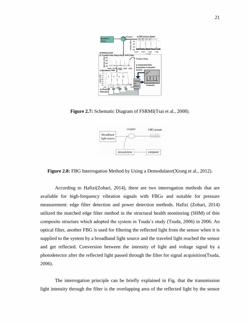
Figure 2.7: Schematic Diagram of FSRMI(Tsai et al., 2008).
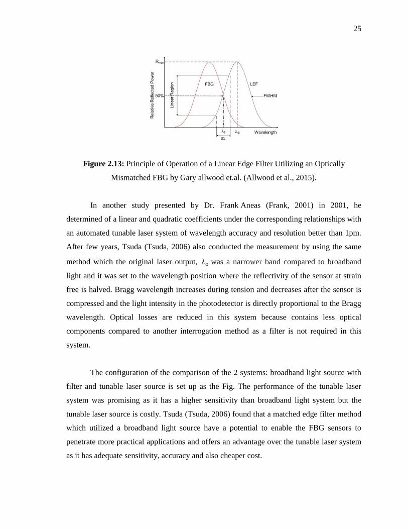
Figure 2.8: FBG Interrogation Method by Using a Demodulator(Xiong et al., 2012).
According to Hafizi(Zohari, 2014), there are two interrogation methods that are
available for high-frequency vibration signals with FBGs and suitable for pressure
measurement: edge filter detection and power detection methods. Hafizi (Zohari, 2014)
utilized the matched edge filter method in the structural health monitoring (SHM) of thin
composite structure which adopted the system in Tsuda’s study (Tsuda, 2006) in 2006. An
optical filter, another FBG is used for filtering the reflected light from the sensor when it is
supplied to the system by a broadband light source and the traveled light reached the sensor
and get reflected. Conversion between the intensity of light and voltage signal by a
photodetector after the reflected light passed through the filter for signal acquisition(Tsuda,
2006).
The interrogation principle can be briefly explained in Fig. that the transmission
light intensity through the filter is the overlapping area of the reflected light by the sensor

22
and transmitted light by the filter. Bragg wavelength reflected from the sensor which in
tension is longer than original Bragg wavelength and shorter as the sensor is subjected to a
compression.
Figure 2.9: Matched Edge Filter Arrangement for Dynamic Sensing by Tsuda(Tsuda,
2006).
Figure 2.10: Schematic Diagram of the Movement of Light in the Circulator-based System
by Hafizi(Zohari, 2014).

23
(a) The Optical Signal at Strain Free
(b) Optical Signal during FBG Sensor in Tension.
(c) Optical Signal during FBG Sensor in Compression.
Figure 2.11: The Resultant of the Optical Signal through an FBG Filter in Matched
Edge Filter Method Proposed by Tsuda (Tsuda, 2006).

24
In 2013, Wild and Richardson developed a numerical model for intensity based
interrogation of FBGs(Wild & Richardson, 2013). By using a laser light source, the
reflected intensity from an FBG can be determined. This method called as power detection.
After power detection method was introduced in their study, Gary Ellwood et al(Allwood,
Wild, Lubansky, & Hinckley, 2015),2015 adopted this method to model the reflected
intensity from two FBGs using a broadband light source in his study due to the reflected
signal from the FBGs are Gaussian, as is the signal from a laser. In Wild and Richardson’s
study(Wild & Richardson, 2013), they have been using a linear edge filter detection.
Therefore, Gary allwood et al(Allwood et al., 2015) decided to use linear edge filter
detection technique for the approximation of their proposed system. A reference FBG
sensor can act as an optical filter to convert the wavelength shift into an optical intensity in
the linear edge filter detection method. The sensitivity and dynamic range of the
interrogation system can be examined from a slope of the filter or full-width half-maximum
(FWHM) of the reference FBG spectrum.
An optically mismatched FBG is used in Gary allwood et al’s study(Allwood et al.,
2015). Reflected intensity will increase from 0% to 100% as the Bragg wavelength
spectrum of the FBG sensors passed across the filter, both spectrums overlapped from 20%
to 80% gave a linear total intensity response in his study. Thus, he concluded that edge
filter detection(Yun-Jiang Rao, 1997) is one of the simplest and most cost-effective among
the interrogation techniques and enables the transducer to be directly connected to an
electronic controller such as a Programmable Logic Controller (PLC) in a plug and play
fashion (Allwood et al., 2015).
Figure 2.12: A Schematic Diagram of Mismatched Edge Filter by Gary Allwood et.al.
(Allwood et al., 2015).
25
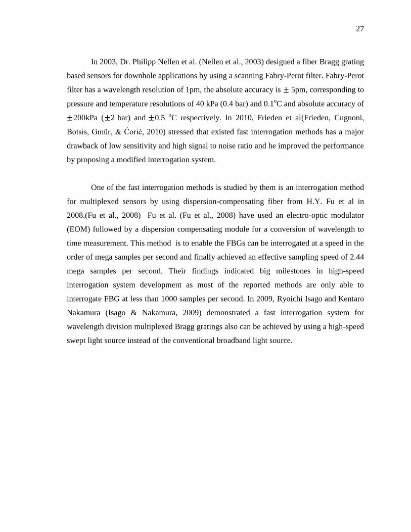
Figure 2.13: Principle of Operation of a Linear Edge Filter Utilizing an Optically
Mismatched FBG by Gary allwood et.al. (Allwood et al., 2015).
In another study presented by Dr. Frank Aneas (Frank, 2001) in 2001, he
determined of a linear and quadratic coefficients under the corresponding relationships with
an automated tunable laser system of wavelength accuracy and resolution better than 1pm.
After few years, Tsuda (Tsuda, 2006) also conducted the measurement by using the same
method which the original laser output, was a narrower band compared to broadband
light and it was set to the wavelength position where the reflectivity of the sensor at strain
free is halved. Bragg wavelength increases during tension and decreases after the sensor is
compressed and the light intensity in the photodetector is directly proportional to the Bragg
wavelength. Optical losses are reduced in this system because contains less optical
components compared to another interrogation method as a filter is not required in this
system.
The configuration of the comparison of the 2 systems: broadband light source with
filter and tunable laser source is set up as the Fig. The performance of the tunable laser
system was promising as it has a higher sensitivity than broadband light system but the
tunable laser source is costly. Tsuda (Tsuda, 2006) found that a matched edge filter method
which utilized a broadband light source have a potential to enable the FBG sensors to
penetrate more practical applications and offers an advantage over the tunable laser system
as it has adequate sensitivity, accuracy and also cheaper cost.

26
(a) Arrangement for FBG Dynamic Sensing Using a Tunable Laser Source.
(b) Variations in Reflectivity at the Lasing Wavelength when the Grating Period
Changes.
Figure 2.14: Principle of Operation for a Detection System Using a Tunable Laser
Source(Tsuda, 2006).
Figure 2.15: An Experimental Setup for Comparison of Two Systems in Ultra
Wave Detection by Tsuda (Tsuda, 2006).
27
In 2003, Dr. Philipp Nellen et al. (Nellen et al., 2003) designed a fiber Bragg grating
based sensors for downhole applications by using a scanning Fabry-Perot filter. Fabry-Perot
filter has a wavelength resolution of 1pm, the absolute accuracy is 5pm, corresponding to
pressure and temperature resolutions of 40 kPa (0.4 bar) and 0.1oC and absolute accuracy of
200kPa ( bar) and 0.5 oC respectively. In 2010, Frieden et al(Frieden, Cugnoni,
Botsis, Gmür, & Ćorić, 2010) stressed that existed fast interrogation methods has a major
drawback of low sensitivity and high signal to noise ratio and he improved the performance
by proposing a modified interrogation system.
One of the fast interrogation methods is studied by them is an interrogation method
for multiplexed sensors by using dispersion-compensating fiber from H.Y. Fu et al in
2008.(Fu et al., 2008) Fu et al. (Fu et al., 2008) have used an electro-optic modulator
(EOM) followed by a dispersion compensating module for a conversion of wavelength to
time measurement. This method is to enable the FBGs can be interrogated at a speed in the
order of mega samples per second and finally achieved an effective sampling speed of 2.44
mega samples per second. Their findings indicated big milestones in high-speed
interrogation system development as most of the reported methods are only able to
interrogate FBG at less than 1000 samples per second. In 2009, Ryoichi Isago and Kentaro
Nakamura (Isago & Nakamura, 2009) demonstrated a fast interrogation system for
wavelength division multiplexed Bragg gratings also can be achieved by using a high-speed
swept light source instead of the conventional broadband light source.

28
Figure 2.16: Structure of High-Speed FBG Interrogation System by H.Y. Fu et al(Fu et al.,
2008).
In Frieden et al’s study on improving the fast interrogation system (Frieden et al.,
2010), strain measurement can be done with a high frequency by coupling the Bragg
reflection spectrum through a tunable Fabry-Perot filter (FP filter). Filtered and unfiltered
Bragg reflection has been measured simultaneously and an intensity ratio is the desired
output signal which is described as a ratio between filtered and unfiltered Bragg reflection
peak. An unfiltered Bragg reflection enables for taking into account of intensity
fluctuations of light sources and losses in the light guide. Strain signal can be obtained
through a discrete calibration curve which demonstrated the relation between intensity ratio
and strain. A spline interpolation function used to find the data points of strain signal from
the obtained curve(Frieden et al., 2010)
In 2013, this method also used by Jun Huang et.al(Huang et al., 2013) to measure
the static and dynamic pressure based on an FBG diaphragm type transducer He mentioned
the FP filter technology is suited for static pressure measurement applications which
required a data acquisition rate of tens of Hz. However, a diffractive grating and charge
coupled device (CCD) array-based FBG interrogator is more viable for their dynamic
pressure measurement as wavelength resolution of 0.4pm and acquisition rate of 8 kHz.
From the figure, a similarity can be observed in Frieden et al(Frieden et al., 2010)
and Tsuda(Tsuda, 2006) in the configuration of both interrogation method. However, types

29
of filter used in the system are different, they are FP filter and matched edge filter
respectively.
Figure 2.17: Fast FBG Interrogation by Frieden et al(Frieden et al., 2010).
(Illustration created by Hafizi(Zohari, 2014))
a tunable optical filter (OTF) is used in Ling et al.’s (Ling, Lau, Cheng, & Jin,
2006) dynamic strain measurement in composite material The operating principle of the
system is similar to Tsuda(Tsuda, 2006) and Frieden et al.(Frieden et al., 2010)’s
interrogation techniques but the type of filter utilized differs. A couple in the OTF system
acted as a Y-type channel to direct the transmitted light to the sensor and reflected light to
OTF in order to generate a voltage output from the detected power of light intensity via the
photodetector then signal analyzer. However, OTP is more expensive compared to matched
edge filter and FP filter.
Figure 2.18: FBG Dynamic Strain Measurement by Ling et al(Ling et al., 2006).
(Illustration created by Hafizi(Zohari, 2014))

30
From a research of FBG pressure sensor, Jun Huang et al.(Huang et al., 2013)
pointed out the intrinsic pressure sensitivity of a bare fiber is too small for the practical
pressure measurement. The value of pressure sensitivity is only 3.04pm/MPa(Xu, Reekie,
Chow, & Dakin, 1993). Strain sensing is the approach for the FBG sensor to have a higher
sensitivity toward pressure. It realized the pressure measurement by installing the sensor
onto an elastic element. The deformation of the primary sensing element, a diaphragm can
stretch the FBG sensor to give out desired wavelength shift for different pressure. A good
design diaphragm can improve the sensitivity and performance of the sensor.
2.10 DIAPHRAGM DESIGN
2.10.1 WORKING PRINCIPLE OF DIAPHRAGM
Elastic deformation of the diaphragm caused by uniformly distributed pressure
which is acting on it. The transverse displacement of the diaphragm is maximum at the core
and minimum at the edges and it is directly proportional to pressure applied. According to
the small deformation theory, the deflection of the hardcore ( ) can be approximately
expressed in Eq. (2.8) (LI, LIU, & WANG, 2006):
P (2.8)
Where P is the applied pressure, is the Poisson’s ratio of the diaphragm material,
E is the Young’s modulus, D is the diaphragm’s diameter, and h represents thickness.

31
Figure 2.19: Circular Diaphragm and Its Strain Distribution Curve(Huang et al., 2013).
2.10.2 EFFECT OF DIAPHRAGM GEOMETRY ON PRESSURE SENSOR’S
PERFORMANCE
The diaphragms with vary in shapes are reacted differently towards the applied
pressure. Those geometries included square, rectangular or circular. A comparison of
performance based on geometry is done by Wang and Ko(Q. Wang & Ko, 1999). He tested
three diaphragm shapes under two ways; with same area or same width by FEA simulations
on stress. The findings show that when the area is equal, the circular diaphragm has the
largest center deflection while the smallest center deflection is the rectangular diaphragm.
The circular diaphragm also has the lowest maximum stress in a comparison with the same
width, therefore, a pressure sensor with the circular diaphragm is able to withstand largest
overload pressure.
For the design consideration, Lynn F. Fuller mentioned in his research(Fuller, 2005)
that larger the size of the diaphragm, lower the pressure range. At the same time, the
pressure range will be higher if the diaphragm is thicker. He stressed that without a proper
design can either damage the diaphragm due to over stress or result in small signal
detection when the diaphragm is too rigid.
The elliptical diaphragm is proposed by Chien Wei-zang et al. (Wei-zang, Li-zhou,
& Xiao-ming, 1992)and S. Timoshenko and S. Woinowsky-Krieger(Timoshenko,
Woinowsky-Krieger, & Woinowsky-Krieger, 1959). Their works are later reviewed by Ali

32
E. Kubba and Kyle Jiang(Kubba & Jiang, 2014) that an elliptical diaphragm may offer
fewer principle stresses, increase pressure range and thermal stresses at the cost of a slight
reduction in sensitivity.
Figure 2.20: Coordinates and Displacements of the Elliptical Plate(Wei-zang et al., 1992).
2.11 TYPES OF DEFORMATION OF THE FBG WITH A DIAPHRAGM-TYPE
PRESSURE TRANSDUCER
Lately, there are several types of the FBG-based sensor has been developed by
researchers (Lihui Liu, Zhang, Zhao, Liu, & Li, 2007; Y. Wang et al., 2010; Yang et al.,
2008). Vengel Rao Pachava et al. (Pachava et al., 2014) used the longitudinal FBG’s
deformation principle by the transverse deflection of the diaphragm which induced an
axially stretched-strain along the length of the FBG thereby creating a red shift of Bragg
wavelength with the increased pressure. However, according to Frantisek Urban et al.
(Urban, Kadlec, Vlach, & Kuchta, 2010), a longitudinal FBG’s deformation will result in
bigger optical signal wavelength displacement (FBG central frequency moves from 10 to
30nm). He also emphasized that by using his method of pressing the FBG laterally, to
obtain an ellipsoidal fiber cross-section shape, which only will generate a maximum of
300pm spectrum peak spread.
In year 2008,Wentao Zhang et al.(Zhang, Li, & Liu, 2009) has reported their new
FBG pressure sensor based on a flat diaphragm with enhanced responsibility by using a
single FBG and an L-shaped lever with a curve of Archimedes spiral then achieved

33
ultrahigh sensitivity, 244 pm/kPa and reduced temperature sensitivity of 2.8 pm/ oC. The L-
shaped lever is made up of quartz glass and laser machined which requires high precision
and the sensor design will be complicated compared to conventional diaphragm transducer.
In the research works (Huang et al., 2013; Lihui Liu et al., 2007; Zhang et al., 2009)
temperature was compensated because a temperature cross-sensitivity can lead to
inaccurate measurement result(Hsu, Wang, Liu, & Chiang, 2006; H.-l. WANG, SONG,
FENG, & WU, 2011). Temperature compensation can increase the accuracy in pressure
measurement.
Yong Zhao et al. (Zhao, Yu, & Liao, 2004) proposed a solution to compensate the
temperature. By adding a reference FBG, D. Sengupta et al. (Sengupta, Sai Shankar, Saidi
Reddy, Sai Prasad, & Srimannarayana, 2012) solved this problem by writing two FBGs in
different diameter fibers. Besides, another solution which combines FBG with Fabry-Perot
cavity is also reported by Yuchi Lin et al. (Y. Lin & Wang, 2009). However, the proposed
pressure transducer in this project works under constant room temperature and the
temperature cross-sensitivity is not being considered.
Figure 2.21: Structure Diagram of Flat Diaphragm FBG Pressure Sensor with Longitudinal
Deformation(Xiong et al., 2012).

34
Figure 2.22: Structure Diagram of Flat Diagram FBG Pressure Sensor with the L-shaped
Lever(Zhang et al., 2009).
Figure 2.23: Structure Diagram of a Flat Diagram of FBG Pressure Sensor with Lateral
Deformation(Huang et al., 2013).
2.12 CHAPTER CONCLUSION
From the research study, FBG have many advantages over conventional pressure
sensor such as piezoelectric and strain gauge. It is light weight, immunity towards chemical
and electromagnetic interference, long distance signal transmission with minimal losses and
it can be multiplexed. Many FBG pressure transducers done by the researchers are in

35
diaphragm type. Flat diaphragm is the suitable primary sensing element for FBG sensor to
enhance the pressure sensitivity.

CHAPTER 3
METHODOLOGY
3.1 INTRODUCTION
This chapter will explain about the concept design that has been made to solve the
problem statement. This chapter will also clarify on the fabrication process, software
implementation including the tests conducted on the dynamic pressure test rig.
3.2 PROJECT FLOW CHART
Figure 3.1 shows the overall flow chart for the project

37
Figure 3.1: Project Flow Chart
Based on the flow chart above, this project is initiated with the identification of the
problem faced in dynamic pressure measurement. The problem has stated, and objectives
are made to find the solution of the problem. Project scope is narrowed down to a particular
field of study after objectives are determined.
Brainstorming for selecting a suitable design for the pressure transducer used in this
project is carried out. The design must be available regarding current resources and
efficient in dynamic pressure sensing. After decided the design, the design has drawn by
using computer aided design software, SolidWorks.

38
The cost of the materials has recorded and bill of material created. Fabrication of
the pressure transducer and test rig is carried out in the next step. Fabrication also included
the installation of fiber Bragg gratings sensor onto the diaphragm.
Testing has started after a dynamic pressure transducer has produced. Analysis and
verification follow data collection. The performance of the FBG sensor on the test rig for
the dynamic response of gas pressure has been observed, and the results are then
documented. A literature review of journals, books, and past studies are used as a reference
in this project to facilitate the research.
3.3 CONCEPT DESIGN
The transducer utilized the elastic deformation of a thin flat diaphragm which can
detect the pressure applied by deforming at the core of the diaphragm. The sensors will be
attached to the diaphragm. FBG senses the deformation and transmit output signal in the
form of electrical. The material is chosen to fabricate a pressure sensor is Aluminium T-
6061. Aluminium has several advantages over others metals which are low weight,
economy and also fabricability. However, most aluminium alloys should not be used above
100oC as the deterioration of the tensile strength occurs rapidly above this temperature.
Therefore, it is suitable for an operating temperature under 100oC
39
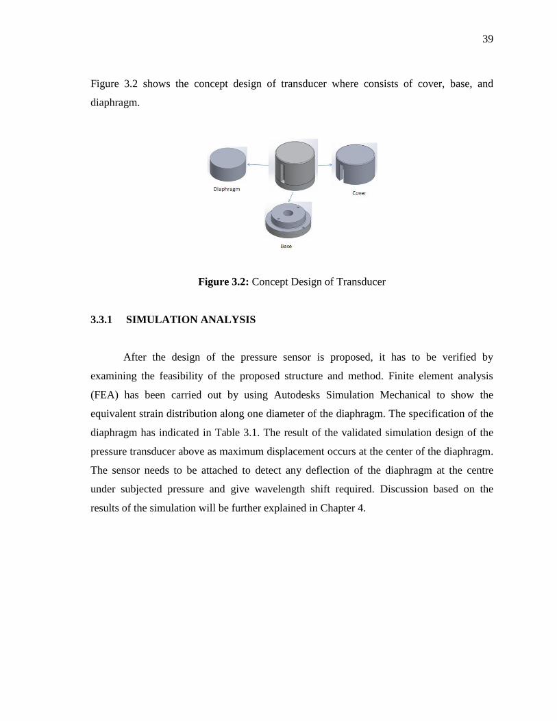
Figure 3.2 shows the concept design of transducer where consists of cover, base, and
diaphragm.
Figure 3.2: Concept Design of Transducer
3.3.1 SIMULATION ANALYSIS
After the design of the pressure sensor is proposed, it has to be verified by
examining the feasibility of the proposed structure and method. Finite element analysis
(FEA) has been carried out by using Autodesks Simulation Mechanical to show the
equivalent strain distribution along one diameter of the diaphragm. The specification of the
diaphragm has indicated in Table 3.1. The result of the validated simulation design of the
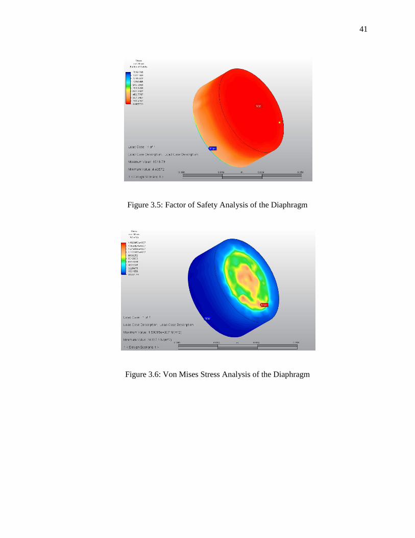
pressure transducer above as maximum displacement occurs at the center of the diaphragm.
The sensor needs to be attached to detect any deflection of the diaphragm at the centre
under subjected pressure and give wavelength shift required. Discussion based on the
results of the simulation will be further explained in Chapter 4.

40
Table 3.1: Specification of Diaphragm
Material Aluminum T-6061 Alloy
Young’s Modulus, E 69×109 N/m
2
Poisson Ratio 0.33
Available Radius 4.5 cm
Thickness 0.06 cm
Figure 3.3: Meshing of the Diaphragm
Figure 3.4: Displacement Analysis of the Diaphragm
41
Figure 3.5: Factor of Safety Analysis of the Diaphragm
Figure 3.6: Von Mises Stress Analysis of the Diaphragm

42
3.4 FABRICATION PROCESS
The next process has done by fabricating the dynamic pressure transducer by using
lathe machine as shown in Figure 3.7. The raw material of the transducer is manufactured
into the desired shape and dimensions part by part in turning process.
Figure 3.7: Lathe Machine
Figure 3.8: Machining in Process

43
(a) (b)
Figure 3.9: Lathed Products, (a) Base and (b) Diaphragm
The diaphragm of the transducer is required to be precisely machined as to reduce
the thickness of the raw material to 1.00 mm in a CNC machining process. A drilling
process followed by adding threads is carried out to enable the screws to fasten the parts.
Before the process started, G code for diaphragm and base are generated by drawing the
part and assigned toolpath in Mastercam X5, software for CNC machining. The toolpath
has to be verified with simulation in the software.
Figure 3.10: CNC Milling Machine

44
(a)
(b)
Figure 3.11: Drawings in Mastercam X5 (a) Base and (b) Diaphragm
Preparation of tools needed for a process respectively and a workpiece is clamped
firmly to be ready for machining. Origins of the workpiece on x and y-axis and origin of

45
each tools on z-axis are set carefully to avoid any misplace of tools which will damage the
cutting tools when it collides onto the workpiece. Then, the last step is posting codes of all
the tool paths in NC file to communicate with the CNC milling machine. The process is
repeated for the second part.
(a) (b)
Figure 3.12: (a) and (b) Types of Tools Used
Figure 3.13: Calibration of Tool on Z-axis

46
(a) (b)
Figure 3.14: CNC Finished Products (a) Diaphragm and (b) Base
For the cover of the pressure transducer, time and cost are saved by using rapid
prototyping, 3D printing. The material of the filament used is Acrylonitrile Butadiene
Styrene (ABS). Silicon glue is used as an adhesive to bond the diaphragm element to the
base for eliminating leakage problem and shown in figure 3.15.
Figure 3.15: Assembly of the Pressure Transducer

47
Figure 3.16: 3D Printed Cover
Commercially available FBG was used with a reflective wavelength of about
1546.97nm. Installation of the FBG sensor on the diaphragm is done by using epoxy glue.
The fragile bare FBG is encapsulated by heat shrinkable tube. During the installation, it is
highly recommended to press on the sensor to the diaphragm as long as possible. In this
case, pressed it for 1 minute to ensure the FBG sensor has perfect bonded to the structure.
Imperfect bonding may cause inaccuracy in sensing. Then, it is ready to be tested in the
experimental stage.
Figure 3.17: FBG Dynamic Pressure Transducer

48
3.5 INTERROGATION SYSTEM
In this project, matched edge interrogation method is incorporated to convert optical
output to electrical output as the sensor sensed a change in strain of the pressure transducer
when pressure is applied. A matched edge interrogation method consists of ASE light
source, an optical circulator, filter, a photodetector and an NI-DAQ unit. Figure 3.18 shows
the arrangement of the interrogation system to enable data acquisition on the computer. The
matched edge filter interrogation method used in this experiment makes cheap interrogation
method for FBG possible without sacrificed the accuracy measurement of the output
voltage. It can reduce the overall cost of the sensing system since the market product solid
state FBG interrogator is expensive. Interrogation of FBG is enabling the optical signal to
be converted to an electrical signal. Therefore, the transducer can be easily connected to a
data acquisition unit or an electronic controller, such as Programmable Logic Controller
(PLC).
Figure 3.18: Matched Edge Interrogation System

49
3.6 EXPERIMENTAL SETUP
The experiment procedure for the FBG and strain gauge dynamic pressure
transducer in dynamic response can be divided into two subchapters; the methods in a
calibration of FBG sensor and also dynamic sensing in pipe leak test. The experiment of
the calibration is explained in section 3.7.1 while the latter is explained in section 3.7.2.
3.6.1 CALIBRATION
Before any testing to be carried out by using this FBG dynamic pressure transducer,
the specification and capabilities of the FBG are known via calibration process. The
sensitivity of the FBG on pressure sensing can be obtained from the graph which
documented the relationship between pressure and wavelength shift in FBG sensor. The
pressure will increase gradually to apply strain to the FBG sensor through the deformation
of the diaphragm. Broadband signal from an amplified spontaneous emission (ASE) source
is launched into the FBG through port 1to 2 of the optical circulator. A narrow band
wavelength of the FBG after sensing the pressure will be reflected. Then, routed into an
optical spectrum analyze through port 2 to 3 of the optical circulator. The OSA monitored
the reflected spectrum from the sensing FBG, and it is correlated to the pressure gauge’s
reading. Be noted that the entire experiment is carried out at the room temperature, 23oC as
this project is not assessing the temperature compensation of the pressure transducer based
on FBG sensor.
The experiment is repeated several times with pressure rise and drop of 0.5 bar to
demonstrate the repeatability of the diaphragm-type transducer then repeatability error is
tested. A linear relationship is expected, pressure sensitivity and fitting linear correlation
coefficient can be calculated from the slope in the graph.

50
Figure 3.19: Air Compressor
Figure 3.20: Calibration Test Rig
Figure 3.19 shows an air compressor is used in this experiment as a pressure input
to the test rig. The test rig is made up of PVC pipe and fitted with a pressure gauge to
display the pressure inside the pipe. A dynamic pressure sensor is being installed to detect
the pressure applied to calibrate both strain gauge and FBG sensor before real application
on dynamic pressure measurement. By using a compressor, the pressure inside the test rig
is varied in steps of 0.5 bar concerning a precision pressure gauge which installed on the
same test rig. The sensors are connected to NI-DAQmx in a computer to acquire a signal
and parse for further processing and analyzing in DasyLAB software. A serial cable of the
51
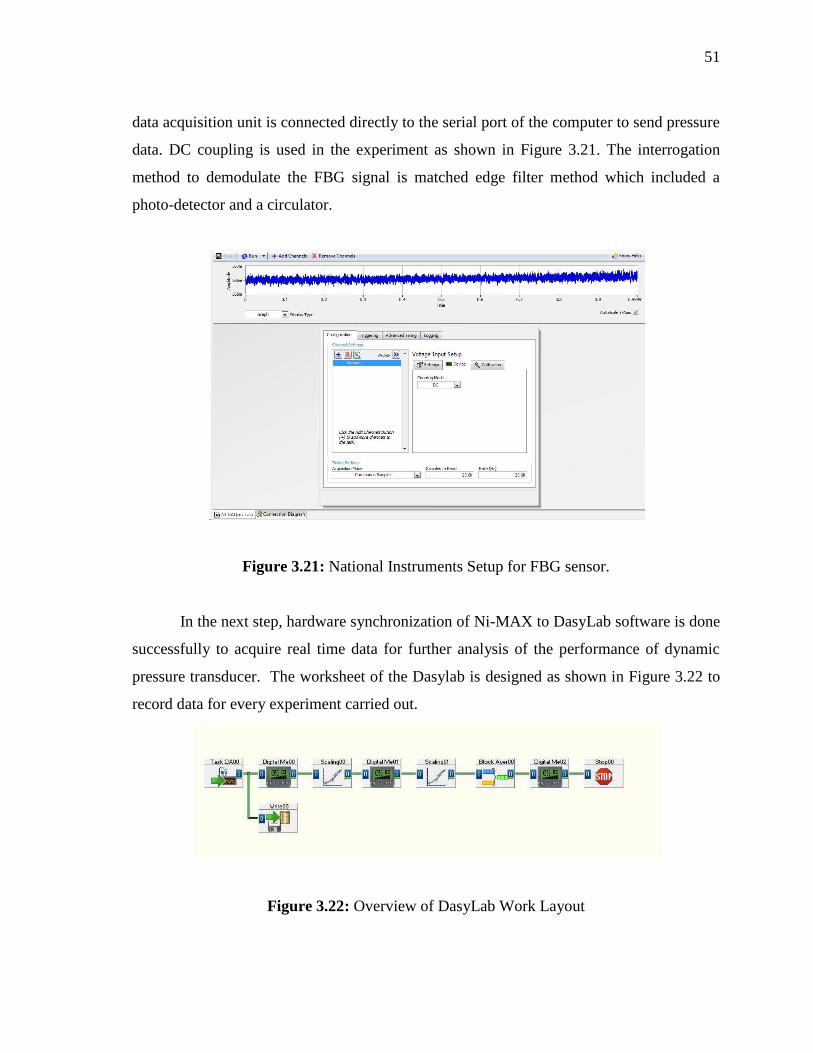
data acquisition unit is connected directly to the serial port of the computer to send pressure
data. DC coupling is used in the experiment as shown in Figure 3.21. The interrogation
method to demodulate the FBG signal is matched edge filter method which included a
photo-detector and a circulator.
Figure 3.21: National Instruments Setup for FBG sensor.
In the next step, hardware synchronization of Ni-MAX to DasyLab software is done
successfully to acquire real time data for further analysis of the performance of dynamic
pressure transducer. The worksheet of the Dasylab is designed as shown in Figure 3.22 to
record data for every experiment carried out.
Figure 3.22: Overview of DasyLab Work Layout
52
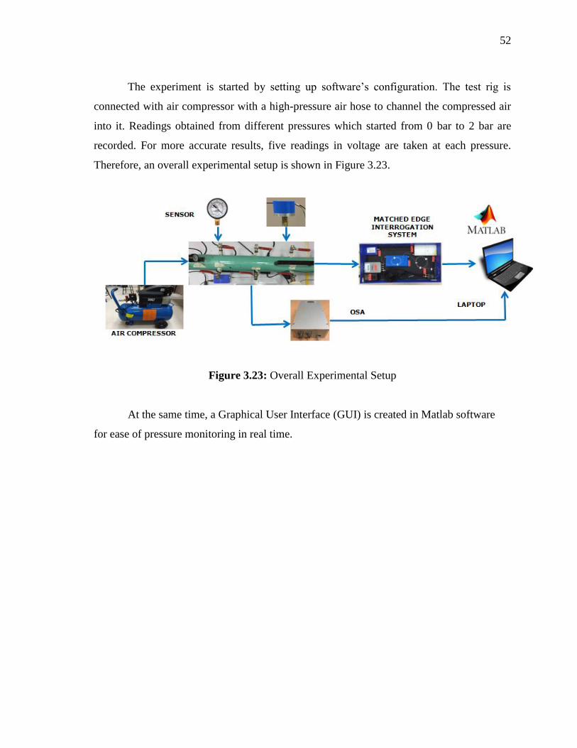
The experiment is started by setting up software’s configuration. The test rig is
connected with air compressor with a high-pressure air hose to channel the compressed air
into it. Readings obtained from different pressures which started from 0 bar to 2 bar are
recorded. For more accurate results, five readings in voltage are taken at each pressure.
Therefore, an overall experimental setup is shown in Figure 3.23.
Figure 3.23: Overall Experimental Setup
At the same time, a Graphical User Interface (GUI) is created in Matlab software
for ease of pressure monitoring in real time.

53
Figure 3.24: Matlab’s GUI
3.6.2 PIPE LEAK TEST
After the specification of the dynamic pressure transducer is identified, it is tested
on a well-controllable test rig about its dynamic response. A leak in the pipeline occurs
with a sudden decrease in the pressure. It will generate a pressure pulse which travels
upstream and downstream through the pipe as a wave. The performance of the FBG and
strain gauge toward rapid pressure changes will be compared to prove that FBG is an
alternative sensing element which can provide robust measurement in dynamic sensing than
strain gauge.
54
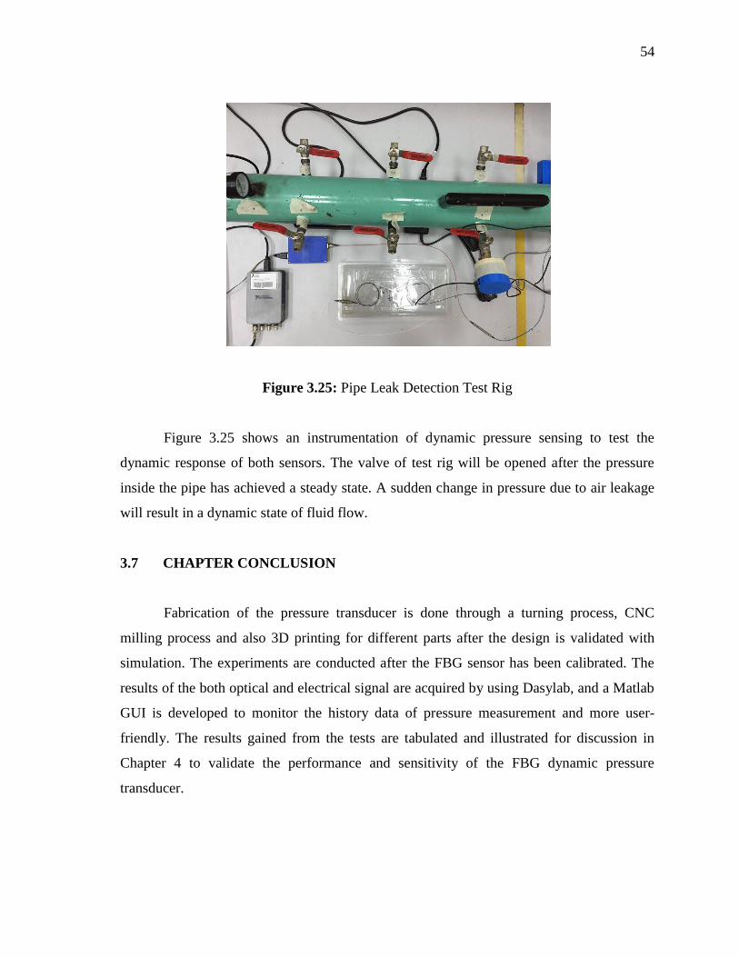
Figure 3.25: Pipe Leak Detection Test Rig
Figure 3.25 shows an instrumentation of dynamic pressure sensing to test the
dynamic response of both sensors. The valve of test rig will be opened after the pressure
inside the pipe has achieved a steady state. A sudden change in pressure due to air leakage
will result in a dynamic state of fluid flow.
3.7 CHAPTER CONCLUSION
Fabrication of the pressure transducer is done through a turning process, CNC
milling process and also 3D printing for different parts after the design is validated with
simulation. The experiments are conducted after the FBG sensor has been calibrated. The
results of the both optical and electrical signal are acquired by using Dasylab, and a Matlab
GUI is developed to monitor the history data of pressure measurement and more user-
friendly. The results gained from the tests are tabulated and illustrated for discussion in
Chapter 4 to validate the performance and sensitivity of the FBG dynamic pressure
transducer.

CHAPTER 4
RESULTS AND DISCUSSIONS
4.1 INTRODUCTION
In this chapter, the results obtained for dynamic pressure sensing via Matlab will be
interpreted, and the reason behind its limitations will also be discussed as well.
4.2 RESULTS
4.2.1 OPTICAL SIGNAL
During the experiment, the pressure applied to the pressure transducer by the
compressor is changed from 0 bar to 5 bar with a step of 0.5 bar under a fixed temperature
at the room temperature. The dynamic pressure transducer is connected to the Optical
Spectrum Analyzer (OSA) to observe the wavelength shift and associated peak power
under different pressure applied to it by using computer software, Sense2020. The output of
the sensor in the computer is shown in Figure 4.1. The results are plotted in Figure
4.2.Once the FBG sensor detected the deformation of the diaphragm caused by the pressure
exerted, the grating period and fiber index of the sensor change. The detected strain is then
coded into a wavelength in a direct way and caused a shift in Bragg wavelength of the
FBG. Thus, a narrowband matched wavelength is reflected to the OSA, and the remaining
wavelengths are transmitted to the circulator in the interrogation system for continuous
sensing. It can be observed from Figure 4.2 that the variation

56
of the Bragg wavelength under the increased pressure is linear and exhibited no
considerable change in the peak power levels. Figure 4.4 verified FBG is stretched and
detected the positive strain. The variation pattern is linear at room temperature, and the
slope is 12.273, and the fitting linear correlation coefficient reached 99.91%. The
experimentally measured pressure sensitivity is evaluated as high as 106 pm/bar from the
fitting result presented in Figure 4.3.
Figure 4.1: OSA Output in Sense2020

57
Figure 4.2: The Spectra of Bragg Wavelength Shift of the Sensing FBG at Different
Applied Pressure Values 0 Until 5 bar, Respectively
Figure 4.3: Variation of Wavelength of FBG versus Pressure
0
2000
4000
6000
8000
10000
12000
14000
1543.75 1544.25 1544.75 1545.25 1545.75
Inte
nsi
ty (
AU
)
Bragg Wavelength(nm)
0 bar
1 bar
2 bar
3 bar
4 bar
5 bar
filter
y = 0.1227x + 1544.4 R² = 0.9991
1544.4
1544.5
1544.6
1544.7
1544.8
1544.9
1545
1545.1
0 1 2 3 4 5 6
Wav
ele
ngt
h (
nm
)
Pressure (bar)
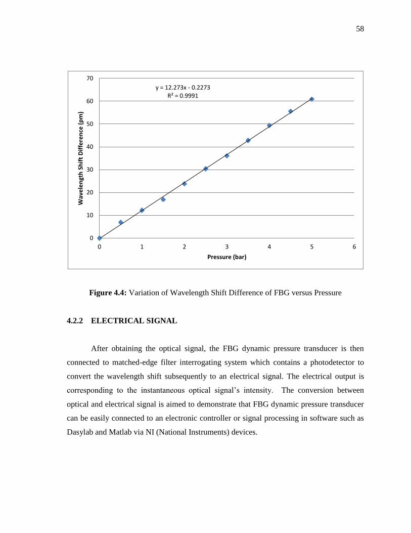
58
Figure 4.4: Variation of Wavelength Shift Difference of FBG versus Pressure
4.2.2 ELECTRICAL SIGNAL
After obtaining the optical signal, the FBG dynamic pressure transducer is then
connected to matched-edge filter interrogating system which contains a photodetector to
convert the wavelength shift subsequently to an electrical signal. The electrical output is
corresponding to the instantaneous optical signal’s intensity. The conversion between
optical and electrical signal is aimed to demonstrate that FBG dynamic pressure transducer
can be easily connected to an electronic controller or signal processing in software such as
Dasylab and Matlab via NI (National Instruments) devices.
y = 12.273x - 0.2273 R² = 0.9991
0
10
20
30
40
50
60
70
0 1 2 3 4 5 6
Wav
ele
ngt
h S
hif
t D
iffe
ren
ce (
pm
)
Pressure (bar)

59
Figure 4.5: Output Voltage of the Sensor from 0 to 5 bar
Figure 4.5 shows the relationship between output voltage and the pressure applied
to the transducer in a linear region. The range of linearity of the transducer is 0 to 2 bar by
using the interrogation method with another FBG acts as a filter. From the result obtained
as above, the linear range of the pressure measurement based on electrical signal is affected
by the choice of filter FBG. When the pressure applied passed 3.0 bar, there is a turning
point which the output reading is in increasing trend. It can be illustrated in Figure 4.6, 4.7
and 4.8 to show that the behavior of transmission of wavelength to the photodetector.
0.47
0.48
0.49
0.5
0.51
0.52
0.53
0.54
0.55
0.56
0 1 2 3 4 5 6
Vo
ltag
e (
V)
Pressure (bar)

60
(a)
(b)

61
(c)
Figure 4.6: Wavelength Variation from (a) 0 bar, (b) 1 bar and (c) 2 bar
The shaded region in the figure represented the intensity of the reflected wavelength
from the FBG sensor will be transmitted to the photodetector. As the wavelengths become
longer or shift to the right, the area of the shaded region decreases so as the intensity
transmitted to the photodetector. Therefore, the output voltage from the photodetector to the
data acquisition unit is reduced when the photodiode inside the photodetector sense less
light intensity.
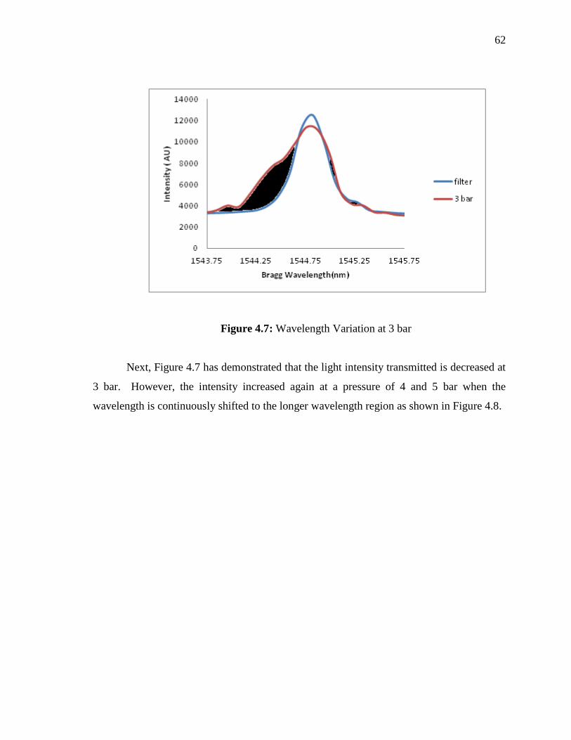
62
Figure 4.7: Wavelength Variation at 3 bar
Next, Figure 4.7 has demonstrated that the light intensity transmitted is decreased at
3 bar. However, the intensity increased again at a pressure of 4 and 5 bar when the
wavelength is continuously shifted to the longer wavelength region as shown in Figure 4.8.

63
(a)
(b)
Figure 4.8: Wavelength Variation from (a) 4 and (b) 5 bar
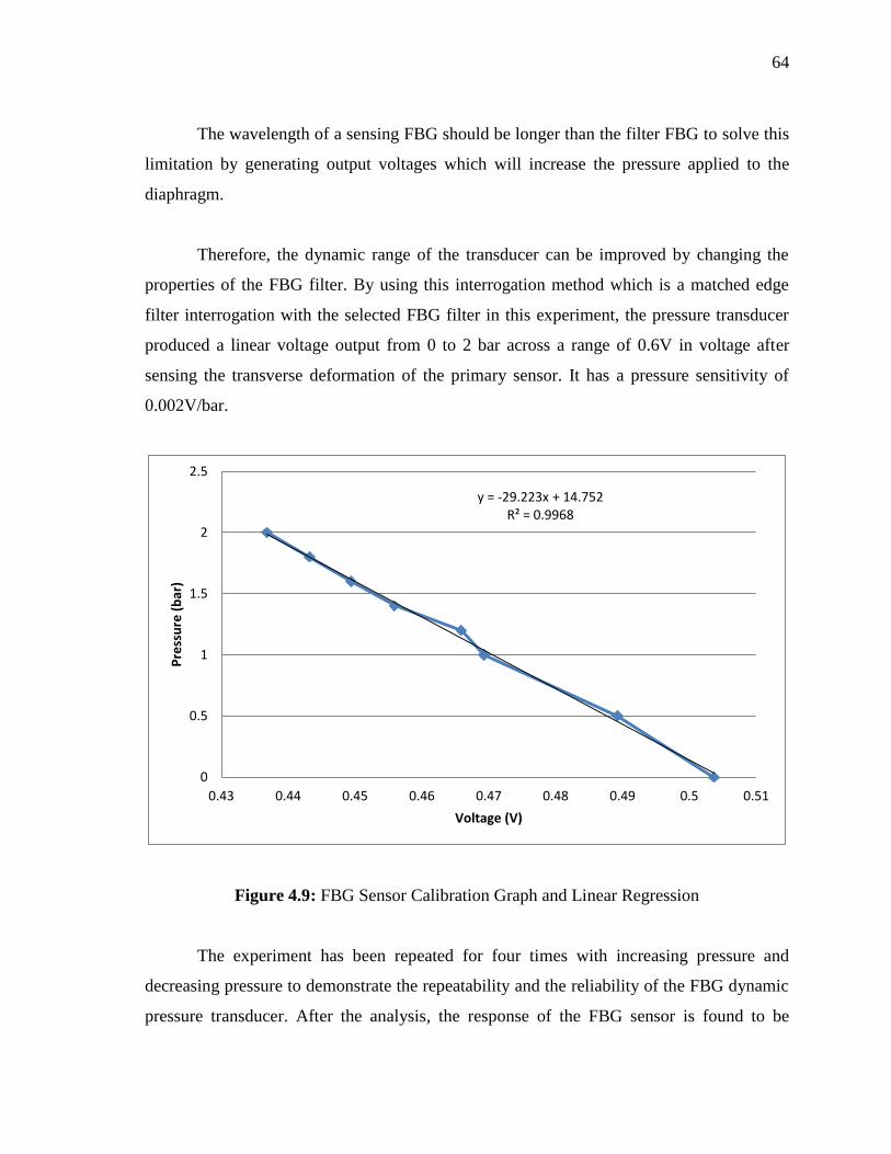
64
The wavelength of a sensing FBG should be longer than the filter FBG to solve this
limitation by generating output voltages which will increase the pressure applied to the
diaphragm.
Therefore, the dynamic range of the transducer can be improved by changing the
properties of the FBG filter. By using this interrogation method which is a matched edge
filter interrogation with the selected FBG filter in this experiment, the pressure transducer
produced a linear voltage output from 0 to 2 bar across a range of 0.6V in voltage after
sensing the transverse deformation of the primary sensor. It has a pressure sensitivity of
0.002V/bar.
Figure 4.9: FBG Sensor Calibration Graph and Linear Regression
The experiment has been repeated for four times with increasing pressure and
decreasing pressure to demonstrate the repeatability and the reliability of the FBG dynamic
pressure transducer. After the analysis, the response of the FBG sensor is found to be
y = -29.223x + 14.752 R² = 0.9968
0
0.5
1
1.5
2
2.5
0.43 0.44 0.45 0.46 0.47 0.48 0.49 0.5 0.51
Pre
ssu
re (
bar
)
Voltage (V)

65
consistent. The results obtained from the repeatability test are presented in Figure 4.10. The
repeatability error for pressure measurement is found to be 0.0015V, which is less than
0.3%.
Figure 4.10: Repeatability of the Transducer
4.3 DYNAMIC RESPONSE DURING A LEAKAGE
The dynamic pressure transducer is subjected to an air leakage condition to test the
dynamic response of the FBG sensor under a rapid change of pressure inside the test rig.
The coupling mode of the NI-max is altered to AC coupling to observe the variations in the
signal transmitted. The photodetector amplification is set at 20dB. The response after
detected an air leakage during a pipe flow is recorded in Figure 4.11. A valve of the test rig
is opened to imitate the leaking situation, and a sudden decrease in the applied internal
pressure caused the diaphragm to be reduced in its deformation as less force exerted on it
during a leakage when the air is escaped to the surrounding. At the same time, the FBG
0.48
0.49
0.5
0.51
0.52
0.53
0.54
0.55
0.56
0 0.5 1 1.5 2 2.5
Vo
ltag
e (
V)
Pressure (bar)
Repeatability Response
1st Pressure Increment
1st Pressure Decrement
2nd Pressure Increment
2nd Pressure Decrement

66
experienced a negative strain when the diaphragm retracted. Therefore, the Bragg
wavelength also reduced and results in a variation of output voltage after the reflected
Bragg wavelength passed through the interrogator.
Figure 4.11: Dynamic Response of FBG Sensor during a Pipe Leakage
In Figure 4.11, the first instantaneous peak response in the graph indicates a valve is
opened to simulate the leaking situation while the similar instantaneous second peak
occurred when the valve is closed, and the pressure inside the test rig is recovered to initial
pressure.
4.4 DATA VALIDATION WITH PRESSURE GAUGE
Mechanical gauges are using bourdon tube as a sensing element in pressure
measurement, and pressure is the only source of energy to indicate the measured static
pressure visually. The elastic chamber is placed inside the gauge case, and it will move
after sensing the pressure hence the output from the mechanical gauges is motion. Other
than bellows and single or multi-capsule stacks, Bourdon tubes are also the common used
elastic chambers in the pressure gauge for the fluid power system. However, pressure
gauges with Bourdon tube have been used for many applications commonly nowadays
when compared to bellows and stacks.

67
The Bourdon tube consists of several types which are C-shaped, spiral and helical.
The C-shaped Bourdon changes its flattened cross section by the excess pressure in the tube.
The sealed tip of the bourdon tube moves a short distance then transmitted a motion to a
great train which can rotate the indicating pointer. A pointer displays the pressure on a
graduated scale to display the detected pressure. Figure 4.12 shows the structure of the C-
shaped Bourdon tube for better illustration of its working principle. The distance of the tip
moves depends on the size of the tube. A pressure gauge used in this experiment is to test
the accuracy of the FBG pressure transducer.
Figure 4.12: Structure of a C-Shaped Bourdon Tube Pressure Gauge("Engineering
Essentials: Pressure Gauges & Flow Meters,")
The experiment is carried out by adjusting the pressure in the air compressor, and
pressurized air is channeled to the test rig under testing. A pressure gauge and FBG
pressure transducer are both installed at the openings to measure the pressure inside the test
rig. The results from both measuring instruments are tabulated in Table 4.1, and errors
between two output readings are calculated. The average error for 11 pressure measurement
is found to be 1.30%. From the result, we can conclude that the FBG dynamic pressure
transducer has good accuracy and high reliability in measuring pressure. Mind that pressure
gauge reading in this experiment will be affected by parallax error and zero error.

68
Table 4.1: Summarized Data of Comparison between Pressure Gauge and FBG Sensor
Sampl
e
Pressure Gauge
Reading(bar)
FBG Dynamic Pressure Transducer
Readings (bar)
Error
(%)
1 0 -0.01 1.00
2 0.4 0.4 0.00
3 0.58 0.59 1.70
4 0.55 0.55 0.00
5 1.8 1.78 1.10
6 1.65 1.62 1.18
7 1.3 1.29 1.00
8 0.85 0.85 0.00
9 0.89 0.93 4.00
10 0.48 0.47 2.08
11 0.43 0.44 2.32
Average Error 1.30
Figure 4.13: Data Validation with Pressure Gauge
-0.2
0
0.2
0.4
0.6
0.8
1
1.2
1.4
1.6
1.8
2
1 2 3 4 5 6 7 8 9 10 11
Pre
ssu
re (
bar
)
Sample
Pressure Gauge
FBG Pressure Transducer
69
4.5 EFFECT OF THE AMPLIFICATION OF THE PHOTODETECTOR
The photodetector in this project is set at 10dB because the data acquisition unit
only can measure up to 5V once the signal to noise ratio is increased up to 40dB, the
maximum output voltage is remained at 5V without any changes in output voltage when the
pressure is increased. 20dB is tested to measure the output voltage under different pressure.
It showed unstable output signal and larger fluctuation compared to 10dB.
4.6 SIMULATION RESULTS OF THE PRESSURE TRANSDUCER
Simulation results from the finite element analysis are collected and tabulated in
Table 4.2 to assess the maximum pressure can be exerted onto the diaphragm in an
application. A factor of safety is required to be considered as the factor of safety must more
than 1.0 to ensure a safe operation pressure for the pressure transducer. The maximum
factor of safety is at the base of the diaphragm and minimum factor of safety is at the center
of the diaphragm because it is the thinnest part of the structure and experienced maximum
stress and displacement. Therefore, minimum factor of safety has taken into account during
the design to decide the permissible operating pressure or load without catastrophic failure.
Usually, a structure required a factor of safety is 1.5 but above than 2.0, and the structure
will be safer. The designed pressure transducer should be implemented in an application
which operates within a pressure range from 0 to 11 bar.

70
Table 4.2: Factor of Safety (FOS) of Diaphragm
Pressure Applied (bar) Factor of Safety
5 4.4857
6 3.7381
7 3.2041
8 2.8062
9 2.4944
10 2.2450
11 2.0409
12 1.8708
13 1.7269
14 1.6035
15 1.4966
16 1.4031
17 1.3206
18 1.2472
19 1.1816
20 1.1225
21 1.0690
22 1.0204
23 0.9761
24 0.9354
4.7 NORMALIZED SIGNAL OUTPUT
The accuracy of the sensor can only be maintained if it is well-calibrated. However,
the initial voltage of the FBG sensor at 0 bar is not the same on different days in an
increasing trend. Few sets of data are observed and illustrated in Figure 4.14 for five days

71
to examine the variability. Before experiments have been conducted, the sensor is pre-
calibrated and the sensor required for adjusting calibration coefficients over time for long-
term application in pressure measurement. To solve this problem, normalization of sensed
data can help to eliminate the variability caused by possible degradation and inconsistency
of broadband light power over time. From Table 4.3, a calibration curve is obtained by
averaging the coefficients in 5 equations with a function of y=-0.0581x+0.9954.
Normalization step is dividing the voltage with initial voltage to limit the data within 0 and
1.
(4.1)
Figure 4.14: Daily Calibration Record
0.4
0.45
0.5
0.55
0.6
0 0.5 1 1.5 2 2.5
Vo
ltag
e (
V)
Pressure (bar)
23-Mar
15-Apr
18-Apr
19-Apr
20-Apr

72
Figure 4.15: Normalized Voltage against Pressure
Table 4.3: Calibration Curve on Different Days
Date Curve Equation Regression
23-Mar y = -0.0662x + 0.9994 0.9976
15-Apr y = -0.0496x + 0.9974 0.9917
18-Apr y = -0.0603x + 0.995 0.9896
19-Apr y = -0.0565x + 0.9943 0.9809
20-Apr y = -0.0577x + 0.9909 0.9784
An experiment has been conducted to validate the feasibility of proposed solution to
solve this calibration problem stated above with the same experimental setup. Before
carrying out the experiment, a modification is done in Matlab GUI to measure the pressure
based on normalized voltage as in Figure 4.16.
0.86
0.88
0.9
0.92
0.94
0.96
0.98
1
1.02
0 0.5 1 1.5 2 2.5
No
rmal
ize
d V
olt
age
(V
)
Pressure (bar)
20-Apr
19-Apr
18-Apr
23-Mar
15-Apr
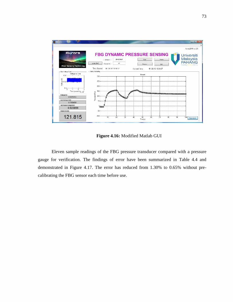
73
Figure 4.16: Modified Matlab GUI
Eleven sample readings of the FBG pressure transducer compared with a pressure
gauge for verification. The findings of error have been summarized in Table 4.4 and
demonstrated in Figure 4.17. The error has reduced from 1.30% to 0.65% without pre-
calibrating the FBG sensor each time before use.
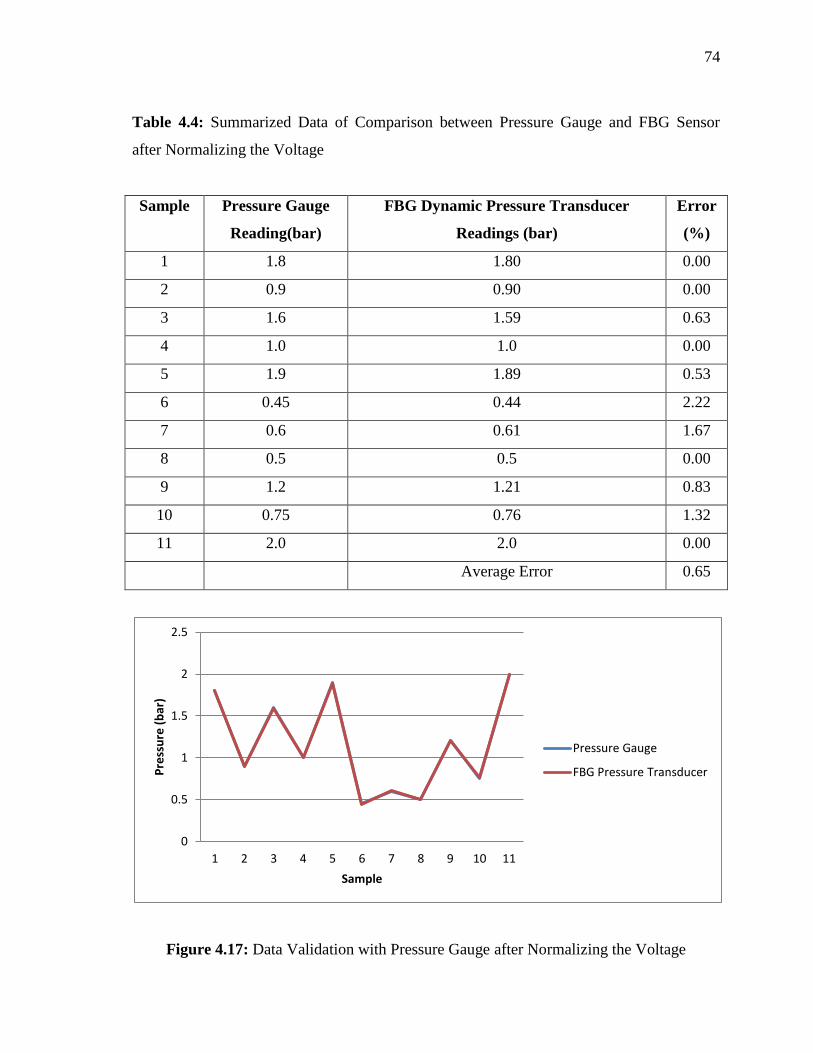
74
Table 4.4: Summarized Data of Comparison between Pressure Gauge and FBG Sensor
after Normalizing the Voltage
Sample Pressure Gauge
Reading(bar)
FBG Dynamic Pressure Transducer
Readings (bar)
Error
(%)
1 1.8 1.80 0.00
2 0.9 0.90 0.00
3 1.6 1.59 0.63
4 1.0 1.0 0.00
5 1.9 1.89 0.53
6 0.45 0.44 2.22
7 0.6 0.61 1.67
8 0.5 0.5 0.00
9 1.2 1.21 0.83
10 0.75 0.76 1.32
11 2.0 2.0 0.00
Average Error 0.65
Figure 4.17: Data Validation with Pressure Gauge after Normalizing the Voltage
0
0.5
1
1.5
2
2.5
1 2 3 4 5 6 7 8 9 10 11
Pre
ssu
re (
bar
)
Sample
Pressure Gauge
FBG Pressure Transducer

75
4.8 CHAPTER CONCLUSION
From the results, the pressure transducer shows pressure sensitivity of106 pm/bar
based on optical signal while 0.002V/bar for an electrical signal after being interrogated
with a matched edge filter system. The repeatability data demonstrated that the sensor has
no significant hysteresis and able to detect dynamic pressure changes in a pipe leak
condition. With comparison to Bourdon tube, the error in the readings is 1.3%.
Normalization of voltage can help to solve inconstant initial voltage output problem by
establishing a calibration equation which will not affect by the initial voltage variability on
a daily basis. Therefore, this approach has minimized the pressure measurement error to
0.65%.
CHAPTER 5
CONCLUSION AND RECOMMENDATION
5.1 INTRODUCTION
In this final chapter, the conclusion is made about the Fiber Bragg Grating dynamic
pressure transducer and some recommendation for further improvement in term of
performance, sensitivity, accuracy and reliability.
5.2 CONCLUSION OF STUDY
In a nutshell, a diaphragm type FBG dynamic pressure transducer has been designed
and demonstrated. The pressure transducer uses an FBG sensor which adhered on the
surface of the diaphragm along the radial direction. FBG sensor experiences a radial strain
which induced by the deflection of the diaphragm. Therefore, it causes the Bragg
wavelength of the FBG shift as the grating period in the fiber core changes. The
experimental result shows that the pressure sensitivity of this FBG sensor is 106 pm/bar.
Besides, the FBG sensor has an excellent linearity with a fitting linear correlation
coefficient of 99.91% in pressure measurement. From the repeatability test, an error is
found to be less than 0.3%. The temperature compensation of the pressure transducer has
not been taken into consideration as the operating temperature is fixed at room temperature.
Although the accuracy of the FBG dynamic pressure transducer is only 98.70%,
nevertheless it proves to be easy, and building cost is low. The objectives of the

77
project are successfully fulfilled. In this pressure measurement system, a matched edge
interrogation system is being utilized to convert pressure related FBG wavelength shift into
corresponding light intensity modulation by using a matched FBG sensor is used as a filter.
This interrogation system is less costly than the solid state interrogators in the market to
introduce a cost-effective FBG pressure sensing system. With these merits, an FBG
pressure transducer can be widely implemented in mainstream industrial applications.
Hence, the designed FBG dynamic pressure transducer can be used to measure pressures
from low to medium range. It has many potential applications such as pressure
measurement in civil engineering, oil and gas industry and highly hazardous or extreme
working environment because it immunes to electromagnetic interference, electrically
passive, nonconductive and chemically inert.
5.2 PROBLEMS
FBG dynamic pressure transducer can measure both static and dynamic pressure
well with few problems. All the objectives are successfully achieved. However, when the
broadband light source is unplugged, the initial voltage reading from the photodetector will
not be the same as previous after restarting the system on the other day. Another problem is
fragile nature of the FBG sensor during the installation and operation as it snaps easily.
Measurement range of the FBG pressure sensor is highly dependent on the Bragg
wavelength of the FBG filter in the interrogation system to demodulate the reflected
wavelength. With the current design of the interrogation system, the FBG dynamic pressure
transducer sensor can only measure pressure up to 2 bar. Several recommendations have
been made to encounter these problems.
5.3 RECOMMENDATION
The performance of the pressure transducer is still not high since voltage reading is
not stable although the pressure measurement based on optical signal exhibits a high
linearity. For future works, some recommendations have been listed to improve the
accuracy, sensitivity, and reliability of the FBG dynamic pressure transducer.

78
i. Inconstant Voltage Reading
Choose a super luminescent diode (SLED) as a light source because the
power output is more stable and higher when comes to a comparison with ASE.
ii. Fragile FBG Sensor
Bare FBG sensor breaks easily. Therefore, encapsulation in a capillary tube
needs to be done to protect the vulnerable FBG sensor from damage.
iii. Low-Pressure Measurement Range
The proper filter has to be chosen to suit the application.
5.4 FUTURE WORKS
Although this thesis has presented the potential of FBG sensor in static and dynamic
pressure measurement, it could be further developed in a number of ways to improve the
FBG pressure transducer to realize the practical industrial applications in the future:
5.4.1 ANALYSIS ON THE MECHANICAL PART
A diaphragm should be analyzed to assess its range of linearity within its elastic
deformation. In an experiment, the pressure will be applied continuously onto the
diaphragm until it shows a plastic deformation when it cannot return to original state after
the unloading the pressure. It can define a pressure range which the diaphragm will remain
in an elastic domain and with sufficient elastic amplitude for accurate measurement of the
pressure transducer. Eliminates overloading is also crucial as it can damage the sensor.

79
5.4.2 TEMPERATURE COMPENSATION OF FBG PRESSURE TRANSDUCER
For a precise strain measurement, it is necessary to study the temperature effects on
FBG pressure sensor to develop a temperature compensated pressure transducer to ensure
the pressure transducer will not have cross-sensitivity with temperature and sense purely
strain. Thermal stress distributed on a diaphragm will change the grating period of the FBG
sensor and alter the wavelength reflected(Huang et al., 2013). An experiment with a
variation of temperature should conduct by controlling the surrounding temperature with a
thermostat to observe the wavelength shift.
5.4.3 A COMPARISON BETWEEN FBG SENSOR AND OTHER ELECTRONIC
SENSORS
An experiment involves both strain gauge and FBG sensor in dynamic sensing
should carry out to compare the accuracy and sensitivity under a rapid change of pressure.
Besides, two sensors can be tested under an electromagnetic interference (EMI)
environment to demonstrate the impacts of EMI toward the pressure sensing performance
of each sensor.

80
REFERENCES
Achuthan, M. (2009). Engineering Thermodynamics 2Nd Ed: PHI Learning Pvt. Ltd.
Allwood, G., Wild, G., Lubansky, A., & Hinckley, S. (2015). A highly sensitive fiber
Bragg grating diaphragm pressure transducer. Optical fiber technology, 25, 25-32.
Applebaum, W. (2003). Encyclopedia of the scientific revolution: from Copernicus to
Newton: Routledge.
Asundi, A. (2011). Digital holography for MEMS and microsystem metrology (Vol. 7):
John Wiley & Sons.
Balkanli, H. (1981). Bourdon tube transducer: Google Patents.
Batchelor, G. K. (2000). An introduction to fluid dynamics: Cambridge university press.
Baukal Jr, C. E. (2012). The John Zink Hamworthy Combustion Handbook: Volume 1-
Fundamentals: CRC Press.
Boyd Jr, J. H. (1930). A MANOMETER FOR THE MEASUREMENT OF SMALL
PRESSURE DIFFERENTIALS AT HIGH PRESSURES1. Journal of the American
Chemical Society, 52(12), 5102-5106.
Bremer, K., Leen, G., Lewis, E., Moss, B. J., Lochmann, S., & Mueller, I. (2014). Pressure
sensor with an interferometric sensor and an in-fiber Bragg grating reference sensor:
Google Patents.
Busch-Vishniac, I. J. (2012). Electromechanical sensors and actuators: Springer Science &
Business Media.
Chen, H. (2010). Fiber optic pressure sensor based on a single-mode fiber F–P cavity.
Measurement, 43(3), 370-374.
Cui, L.-Q., Long, X., & Qin, J.-M. (2015). A bellow pressure fiber optic sensor for static
ice pressure measurements. Applied Geophysics, 12(2), 255-262.
Davis, M., & Kersey, A. (1995). Application of a fiber Fourier transform spectrometer to
the detection of wavelength-encoded signals from Bragg grating sensors. Lightwave
Technology, Journal of, 13(7), 1289-1295.
Edelmann, C. (1999). Pressure measurement--total pressures. CERN EUROPEAN
ORGANIZATION FOR NUCLEAR RESEARCH-REPORTS-CERN, 59-74.
Edwards, A. T. (2000). Comparison of strain gage and fiber optic sensors on a sting
balance in a supersonic wind tunnel. Virginia Polytechnic Institute and State
University.
Engineering Essentials: Pressure Gauges & Flow Meters. (1 Jan 2012 ). Retrieved from
http://hydraulicspneumatics.com/200/FPE/Sensors/Article/False/6438/FPE-Sensors
Eryukhin, A. (1962). Measuring pressures below 10− 3 mm Hg with a compensated
mercury manometer. Measurement Techniques, 5(6), 466-471.
Fallon, R., Zhang, L., Gloag, A., & Bennion, I. (1997). Identical broadband chirped grating
interrogation technique for temperature and strain sensing. Electronics Letters,
33(8), 705-707.
Filloux, J. (1969). Bourdon tube deep-sea tide gauges. Tsunamis in the Pacific Ocean,
edited.
Frank, A. (2001). Dehnungs- und Temperaturmessung in Verbundwerkstoffen mit
eingebetteten faseroptischen Bragg-Gitter-Sensoren. Bericht- Eidgenossische
Materialprufungs- und Forschungsanstalt.

81
Frieden, J., Cugnoni, J., Botsis, J., Gmür, T., & Ćorić, D. (2010). High-speed internal strain
measurements in composite structures under dynamic load using embedded FBG
sensors. Composite Structures, 92(8), 1905-1912.
Fu, H., Liu, H., Dong, X., Tam, H., Wai, P., & Lu, C. (2008). High-speed fibre Bragg
grating sensor interrogation using dispersion-compensation fibre. Electronics
Letters, 44(10), 618-620.
Fuller, L. (2005). Bulk micromachined pressure sensor. Rochester Institute of Technology.
Goldstein, R. (1996). Fluid mechanics measurements: CRC Press.
Grubsky, V., & Feinberg, J. (2000). Long-period fiber gratings with variable coupling for
real-time sensing applications. Optics letters, 25(4), 203-205.
Hill, K., Fujii, Y., Johnson, D. C., & Kawasaki, B. (1978). Photosensitivity in optical fiber
waveguides: Application to reflection filter fabrication. Applied Physics Letters,
32(10), 647-649.
Hill, K. O., & Meltz, G. (1997). Fiber Bragg grating technology fundamentals and
overview. Journal of lightwave technology, 15(8), 1263-1276.
Hilliam, R. (2005). Galileo Galilei: Father of modern science: The Rosen Publishing
Group.
Hsu, Y., Wang, L., Liu, W.-F., & Chiang, Y. (2006). Temperature compensation of optical
fiber Bragg grating pressure sensor. Photonics Technology Letters, IEEE, 18(7),
874-876.
Huang, J., Zhou, Z., Wen, X., & Zhang, D. (2013). A diaphragm-type fiber Bragg grating
pressure sensor with temperature compensation. Measurement, 46(3), 1041-1046.
Isago, R., & Nakamura, K. (2009). A high reading rate fiber Bragg grating sensor system
using a high-speed swept light source based on fiber vibrations. Measurement
science and technology, 20(3), 034021.
Jain, K., Bowers, W., & Schmidt, J. W. (2003). A primary dead-weight tester for pressures
(0.05-1.0) MPa. JOURNAL OF RESEARCH-NATIONAL INSTITUTE OF
STANDARDS AND TECHNOLOGY, 108(2), 135-146.
Jones, R. T., & Dunphy, J. R. (2006). Optical differential pressure transducer utilizing a
bellows and flexure system: Google Patents.
JUNG, J., LEE, Y. W., & LEE, B. (2000). High-resolution interrogation technique for fiber
Bragg grating strain sensor using long period grating pair and EDF. Paper
presented at the Proceedings of SPIE, the International Society for Optical
Engineering.
Kang, S. C., Kim, S. Y., Lee, S. B., Kwon, S. W., Choi, S. S., & Lee, B. (1998).
Temperature-independent strain sensor system using a tilted fiber Bragg grating
demodulator. Photonics Technology Letters, IEEE, 10(10), 1461-1463.
Kang, S. C., Lee, S. B., Choi, S. S., & Lee, B. (1999). A novel demodulation technique for
the wavelength shift of fiber Bragg grating sensors using the I/Q signal processing
scheme. Paper presented at the Lasers and Electro-Optics, 1999. CLEO/Pacific
Rim'99. The Pacific Rim Conference on.
Kennedy, G. C. (1954). Pressure-volume-temperature relations in CO2 at elevated
temperatures and pressures. Amer. J. Sci, 252(4).
Kersey, A. D. (1996). A review of recent developments in fiber optic sensor technology.
Optical fiber technology, 2(3), 291-317.

82
Kersey, A. D., Berkoff, T., & Morey, W. (1993). Multiplexed fiber Bragg grating strain-
sensor system with a fiber Fabry–Perot wavelength filter. Optics letters, 18(16),
1370-1372.
Kersey, A. D., Davis, M. A., Patrick, H. J., LeBlanc, M., Koo, K., Askins, C., . . . Friebele,
E. J. (1997). Fiber grating sensors. Journal of lightwave technology, 15(8), 1442-
1463.
Kizz, J. Z. (2008). 100 Greatest Science Discoveries of All Time. The American Biology
Teacher, 70(3), 175-176.
Knute, W. L., & Bailey, W. H. (1992). Fiber-optic transducer apparatus: Google Patents.
Kubba, A. E., & Jiang, K. (2014). A comprehensive study on technologies of tyre
monitoring systems and possible energy solutions. Sensors, 14(6), 10306-10345.
Kumar, V. (1983). An Instrument for the Measurement of Infrasounds and Subsonic
Disturbances in the Atmosphere. IETE Journal of Research, 29(1), 30-32.
Kumar, V., & Narayana, K. Development of an ANN-based Pressure Transducer.
Kunzler, W., Zhu, Z., Selfridge, R., Schultz, S., & Wirthlin, M. (2008). Integrating fiber
Bragg grating sensors with sensor networks. Paper presented at the
AUTOTESTCON, 2008 IEEE.
LI, C.-j., LIU, R.-x., & WANG, J.-z. (2006). Design of the Monitor Platform Based on the
Principle of Sensor Network [J]. Chinese Journal of Sensors and Actuators, 1, 002.
Lin, W., & Zhang, X. (2006). A novel approach for dynamic pressure transducer based
pipeline leak detection. Paper presented at the Intelligent Control and Automation,
2006. WCICA 2006. The Sixth World Congress on.
Lin, Y., & Wang, W. (2009). A novel fiber Bragg grating sensor with temperature
compensation. Paper presented at the Photonics and Optoelectronics, 2009. SOPO
2009. Symposium on.
Ling, H.-y., Lau, K.-t., Cheng, L., & Jin, W. (2006). Viability of using an embedded FBG
sensor in a composite structure for dynamic strain measurement. Measurement,
39(4), 328-334.
Liu, L., CHEN, W.-m., Zhang, P., Wu, J., & Liu, H. (2012). An Embedded FBG Strain
Sensor for Bridge Cable Tension Measurement. Opto-Electronic Engineering, 39(6),
57-61.
Liu, L., Zhang, H., Zhao, Q., Liu, Y., & Li, F. (2007). Temperature-independent FBG
pressure sensor with high sensitivity. Optical fiber technology, 13(1), 78-80.
López-Amo, M., & López-Higuera, J. M. (2011). Multiplexing techniques for FBG sensors.
Chapter, 6, 99-115.
Majumder, M., Gangopadhyay, T. K., Chakraborty, A. K., Dasgupta, K., & Bhattacharya,
D. K. (2008). Fibre Bragg gratings in structural health monitoring—Present status
and applications. Sensors and Actuators A: Physical, 147(1), 150-164.
Marick, S., Bera, S. K., & Bera, S. C. (2014). A Modified Technique of Flow Transducer
Using Bourdon Tube as Primary Sensing Element. Sensors Journal, IEEE, 14(9),
3033-3039.
Melle, S. M., & Liu, K. (1992). A passive wavelength demodulation system for guided-
wave Bragg grating sensors. IEEE Photonics Technology Letters, 4, 516-518.
Meltz, G., Morey, W. W., & Glenn, W. (1989). Formation of Bragg gratings in optical
fibers by a transverse holographic method. Optics letters, 14(15), 823-825.
83
Mihailov, S. J. (2012). Fiber Bragg grating sensors for harsh environments. Sensors, 12(2),
1898-1918.
Mishra, D. (2014). Experimental Combustion: An Introduction: Crc Press.
Morey, W. W., Meltz, G., & Glenn, W. H. (1990). Fiber optic Bragg grating sensors.
Paper presented at the OE/FIBERS'89.
Munson, B. R., Young, D. F., & Okiishi, T. H. (1990). Fundamentals of fluid mechanics:
New York.
Nellen, P. M., Mauron, P., Frank, A., Sennhauser, U., Bohnert, K., Pequignot, P., . . .
Brändle, H. (2003). Reliability of fiber Bragg grating based sensors for downhole
applications. Sensors and Actuators A: Physical, 103(3), 364-376.
Nichols, D. (1970). Strain gage installation manual.
Othonos, A., & Kalli, K. (1999). Fiber Bragg gratings: fundamentals and applications in
telecommunications and sensing: Artech House.
Pachava, V. R., Kamineni, S., Madhuvarasu, S. S., & Putha, K. (2014). A high sensitive
FBG pressure sensor using thin metal diaphragm. Journal of Optics, 43(2), 117-121.
Pinet, É. (2011). Pressure measurement with fiber-optic sensors: commercial technologies
and applications. Paper presented at the 21st International Conference on Optical
Fibre Sensors (OFS21).
Pitot-static tube. (1927). Google Patents.
Rao, Y.-J. (1997). In-fibre Bragg grating sensors. Measurement science and technology,
8(4), 355.
Rao, Y.-J. (1998). Fiber Bragg grating sensors: principles and applications Optical fiber
sensor technology (pp. 355-379): Springer.
Rose-Innes, A. (1970). An oil manometer for liquid helium vapour pressure measurement.
Journal of Physics E: Scientific Instruments, 3(7), 544.
Sengupta, D., Sai Shankar, M., Saidi Reddy, P., Sai Prasad, R., & Srimannarayana, K.
(2012). Sensing of hydrostatic pressure using FBG sensor for liquid level
measurement. Microwave and Optical Technology Letters, 54(7), 1679-1683.
Shames, I. H., & Shames, I. H. (1982). Mechanics of fluids: McGraw-Hill New York, NY.
Sharma, A. K., & Ojha, A. K. (2012). A Study on Micro-Electro-Mechanical Systems
(MEMS) Sensors & their Applications International Journal of Engineering and
Advance Technology (IJEAT), 1(5).
Shaughnessy, E. J. (2010). Introduction to fluid mechanics.
Shu, Y., Chen, W., Zhang, P., Wu, J., Liu, H., & Zhang, W. NON-DESTRUCTIVE
TESTING OF STRESS DISTRIBUTION IN CABLE ANCHOR.
Stein, E. (2013). The History of Theoretical, Material and Computational Mechanics-
Mathematics Meets Mechanics and Engineering (Vol. 1): Springer Science &
Business Media.
Tang, Y. (2006). Polycrystalline Diamond (poly-C) Technology and Piezoresistive Sensor
Application for Cochlear Prosthesis: ProQuest.
Thony, J.-L., & Vachaud, G. (1980). Automatic measurement of soil-water pressure using a
capacitance manometer. Journal of Hydrology, 46(1), 189-196.
Tilford, C. R. (1992). Pressure and vacuum measurements. Physical methods of chemistry,
6.
Timoshenko, S., Woinowsky-Krieger, S., & Woinowsky-Krieger, S. (1959). Theory of
plates and shells (Vol. 2): McGraw-hill New York.
84
Tsai, P., Sun, F., Xiao, G., Zhang, Z., Rahimi, S., & Ban, D. (2008). A new fiber-Bragg-
grating sensor interrogation system deploying free-spectral-range-matching scheme
with high precision and fast detection rate. Photonics Technology Letters, IEEE,
20(4), 300-302.
Tsuda, H. (2006). Ultrasound and damage detection in CFRP using fiber Bragg grating
sensors. Composites science and technology, 66(5), 676-683.
Urban, F., Kadlec, J., Vlach, R., & Kuchta, R. (2010). Design of a pressure sensor based on
optical fiber bragg grating lateral deformation. Sensors, 10(12), 11212-11225.
Vengal Rao, P., Srimannarayana, K., Sai Shankar, M., Kishore, P., & Ravi Prasad, S.
(2012). Enhanced sensitivity of FBG pressure sensor using thin metal diaphragm.
Paper presented at the Fiber Optics and Photonics (PHOTONICS), 2012
International Conference on.
Verbruggen, T. (2009). Load monitoring for wind turbines. Fibre optic sensing and data
processing.
von Beckerath, A. (1998). WIKA-handbook: Pressure and Temperature Measurement:
WIKA Instrument Corporation.
Walter, P. L. (2004). Air-blast and the science of dynamic pressure measurements. Sound
and Vibration, 38(12), 10-17.
WANG, H.-l., SONG, J., FENG, D.-q., & WU, H.-c. (2011). High temperature-pressure
FBG sensor applied to special environments [J]. Optics and Precision Engineering,
3, 010.
Wang, Q., & Ko, W. H. (1999). Modeling of touch mode capacitive sensors and
diaphragms. Sensors and Actuators A: Physical, 75(3), 230-241.
Wang, T., Yuan, Z., Gong, Y., Wu, Y., Rao, Y., Wei, L., . . . Wan, F. (2013). Fiber Bragg
grating strain sensors for marine engineering. Photonic Sensors, 3(3), 267-271.
Wang, X. X., & Wu, C. Y. (2012). Pressure sensitivity researched on the metal-coated
FBG sensors. Paper presented at the Advanced Materials Research.
Wang, Y., Wang, M., & Huang, X. (2010). High-sensitivity fiber Bragg grating transverse
force sensor based on centroid measurement of polarization-dependent loss.
Measurement science and technology, 21(6), 065304.
Wei-zang, C., Li-zhou, P., & Xiao-ming, L. (1992). Large deflection problem of a clamped
elliptical plate subjected to uniform pressure. Applied Mathematics and Mechanics,
13(10), 891-908.
Wild, G., & Richardson, S. (2013). Numerical modeling of intensity-based optical fiber
Bragg grating sensor interrogation systems. Optical Engineering, 52(2), 024404-
024404.
Wyllie, H. (1956). A McLeod gauge for measuring a wide range of pressures. Journal of
Scientific Instruments, 33(8), 317.
Xiong, Y., He, J., Yang, W., Sheng, L., Gao, W., & Chen, Y. (2012). Research on FBG
pressure sensor of flat diaphragm structure. Paper presented at the Measurement,
Information and Control (MIC), 2012 International Conference on.
Xu, M., Reekie, L., Chow, Y., & Dakin, J. P. (1993). Optical in-fibre grating high pressure
sensor. Electronics Letters, 29(4), 398-399.
Yang, Y., Annamdas, V. G. M., Wang, C., & Zhou, Y. (2008). Application of multiplexed
FBG and PZT impedance sensors for health monitoring of rocks. Sensors, 8(1),
271-289.

85
Yunus, A. C., & Cimbala, J. M. (2006). Fluid mechanics: fundamentals and applications.
Zhang, W., Li, F., & Liu, Y. (2009). Fiber Bragg grating pressure sensor with ultrahigh
sensitivity and reduced temperature sensitivity. Optical Engineering, 48(2), 024402-
024402-024404.
Zhao, Y., Yu, C., & Liao, Y. (2004). Differential FBG sensor for temperature-compensated
high-pressure (or displacement) measurement. Optics & Laser Technology, 36(1),
39-42.
Zhu, Y., & Wang, A. (2005). Miniature fiber-optic pressure sensor. Photonics Technology
Letters, IEEE, 17(2), 447-449.
Zohari, M. H. B. (2014). The Applications of Near Infra-Red Fibre Bragg Grating Sensors
for Wave Propagation Based Structural Health Monitoring of Thin Laminated
Composite Plates. (Doctor of Philosophy), University of Southen Queensland,
Australia
86
APPENDIX A
GANTT CHART
PSM1 Item /Week W1 W2 W3 W4 W5 W6 W7 W8 W9 W10 W11 W12 W13 W14
Chapter 1 Title Briefing
Identify objectives and problem statements
Chapter 2 Literature survey on pressure measurement
Literature survey on pressure transducer
Literature survey on fiber Bragg grating sensor
Literature survey on FBG interrogation system
Chapter 3 Finalization of methodology
Preparation and development of pressure transducer
PSM 2
Chapter 4 Validation with pressure gauge
Experiment and analysis of data from FBG dynamic pressure transducer
Chapter 5 Conclusion
Final report preparation
Final presentation preparation
Planning Actual
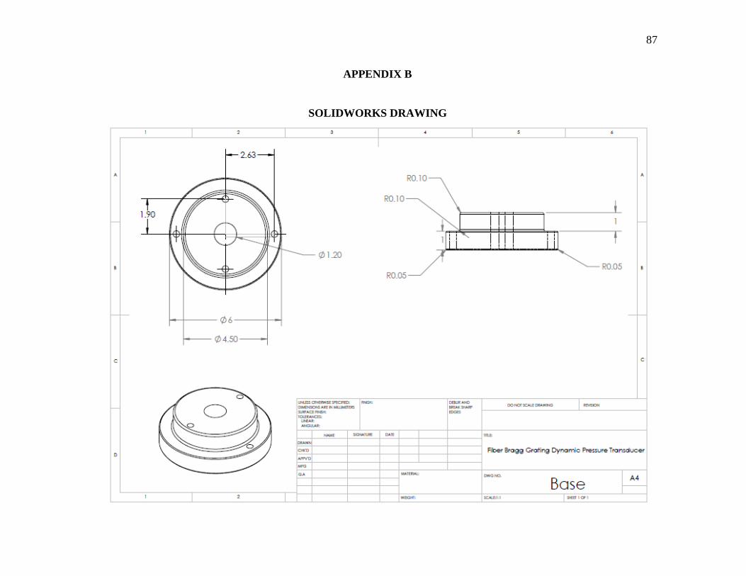
87
APPENDIX B
SOLIDWORKS DRAWING

88
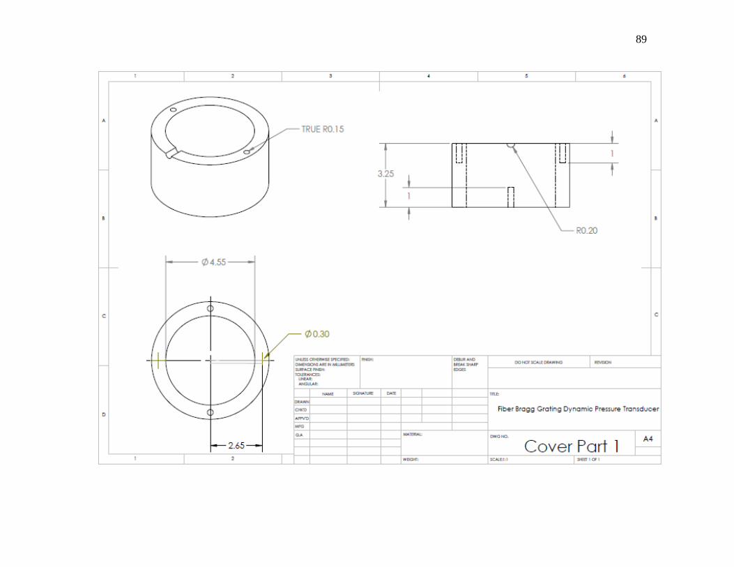
89

90
91
APPENDIX C
MATLAB CODING
function varargout = untitled(varargin)
% UNTITLED MATLAB code for untitled.fig
% UNTITLED, by itself, creates a new UNTITLED or raises the
existing
% singleton*.
%
% H = UNTITLED returns the handle to a new UNTITLED or the handle
to
% the existing singleton*.
%
% UNTITLED('CALLBACK',hObject,eventData,handles,...) calls the
local
% function named CALLBACK in UNTITLED.M with the given input
arguments.
%
% UNTITLED('Property','Value',...) creates a new UNTITLED or
raises the
% existing singleton*. Starting from the left, property value
pairs are
% applied to the GUI before untitled_OpeningFcn gets called. An
% unrecognized property name or invalid value makes property
application
% stop. All inputs are passed to untitled_OpeningFcn via
varargin.
%
% *See GUI Options on GUIDE's Tools menu. Choose "GUI allows
only one
% instance to run (singleton)".
%
% See also: GUIDE, GUIDATA, GUIHANDLES
% Edit the above text to modify the response to help untitled
% Last Modified by GUIDE v2.5 25-May-2016 12:27:58
% Begin initialization code - DO NOT EDIT
gui_Singleton = 1;
gui_State = struct('gui_Name', mfilename, ...
'gui_Singleton', gui_Singleton, ...
'gui_OpeningFcn', @untitled_OpeningFcn, ...
'gui_OutputFcn', @untitled_OutputFcn, ...
'gui_LayoutFcn', [] , ...

92
'gui_Callback', []);
if nargin && ischar(varargin{1})
gui_State.gui_Callback = str2func(varargin{1});
end
if nargout
[varargout{1:nargout}] = gui_mainfcn(gui_State, varargin{:});
else
gui_mainfcn(gui_State, varargin{:});
end
% End initialization code - DO NOT EDIT
% --- Executes just before untitled is made visible.
function untitled_OpeningFcn(hObject, eventdata, handles, varargin)
% This function has no output args, see OutputFcn.
% hObject handle to figure
% eventdata reserved - to be defined in a future version of MATLAB
% handles structure with handles and user data (see GUIDATA)
% varargin command line arguments to untitled (see VARARGIN)
% Choose default command line output for untitled
handles.output = hObject;
% Update handles structure
guidata(hObject, handles);
% UIWAIT makes untitled wait for user response (see UIRESUME)
% uiwait(handles.figure1);
% --- Outputs from this function are returned to the command line.
function varargout = untitled_OutputFcn(hObject, eventdata, handles)
% varargout cell array for returning output args (see VARARGOUT);
% hObject handle to figure
% eventdata reserved - to be defined in a future version of MATLAB
% handles structure with handles and user data (see GUIDATA)
% Get default command line output from handles structure
varargout{1} = handles.output;
axes(handles.axes1);
imshow('Aurora.jpg');
axes(handles.axes4);
imshow('UMP.jpeg');
t=datestr(clock,'dd-mm-yy HH:MM:SS');
set(handles.text10,'String',t,'FontSize',11);
% creating the timer object, so that live mode is possible

93
timer_obj = timer(...
'StartFcn', @user_timer_start, ... % start
function
'TimerFcn', {@user_timer_update, hObject}, ... % timer
function, has to specific the handle to the GUI,
'StopFcn', @user_timer_stop, ... % stop
function
'ErrorFcn', @user_timer_err, ... % error
function
'ExecutionMode', 'fixedRate', ... %
'Period', 0.1, ... % updates
every xx seconds
'TasksToExecute', inf, ...
'BusyMode', 'drop');
% save the timer object as application data
setappdata(hObject, 'timer_obj', timer_obj); % need to
save it because we need to stop and delete it when quit
start(timer_obj);
% UIWAIT makes myClock wait for user response (see UIRESUME)
% uiwait(handles.figure1);
% --- Outputs from this function are returned to the command line.
function varargout = myClock_OutputFcn(hObject, eventdata, handles)
% varargout cell array for returning output args (see VARARGOUT);
% hObject handle to figure
% eventdata reserved - to be defined in a future version of MATLAB
% handles structure with handles and user data (see GUIDATA)
% Get default command line output from handles structure
varargout{1} = handles.output;
function user_timer_update(src,evt, fig_handle)
handles = guihandles(fig_handle);
set(handles.text11, 'string', datestr(now, 'dd-mm-yy
HH:MM:SS'),'FontSize',11);
function user_timer_start(src, evt)
disp('Timer started!');

94
function user_timer_stop(src, evt)
disp('Timer stop');
function user_timer_err(src, evt)
disp('Timer error');
% --- Executes when user attempts to close figure1.
function figure1_CloseRequestFcn(hObject, eventdata, handles)
% hObject handle to figure1 (see GCBO)
% eventdata reserved - to be defined in a future version of MATLAB
% handles structure with handles and user data (see GUIDATA)
% Hint: delete(hObject) closes the figure
stop(getappdata(hObject, 'timer_obj'));
delete(getappdata(hObject, 'timer_obj'));
delete(hObject);
% --- Executes on button press in pushbutton2.
function pushbutton2_Callback(hObject, eventdata, handles)
% hObject handon2 (see GCBO)
% eventdata reserved - to be defined in a future verle to
pushbuttsion of MATLAB
% handles structure with handles and user data (see GUIDATA)
ID=get(handles.edit2,'String');
Channel=get(handles.edit3,'String');
s=daq.createSession('ni');
s.Rate=256000;
s.addAnalogInputChannel(ID,Channel,'Voltage');
k=0;
i=1;
n=0;
while k<100
[data,time]=s.startForeground;
axes(handles.axes5);
plot(data);
set(get(handles.axes5, 'XLabel'), 'String', 'Time (seconds)');
set(get(handles.axes5, 'YLabel'), 'String', 'Voltage (V)');
set(get(handles.axes5, 'Title'), 'String', 'Voltage vs Time');
p=mean(data);
set(handles.text12,'String',p,'FontSize',33);
y=((-29.755*p) + 16.227)*100;
set(handles.text13,'String',y,'FontSize',33);
if(n <=100)
b(i)=y ;

95
i=i+1;
set(gcf,'color','white');
drawnow;
axes(handles.axes8);
plot(b,'-.dk','linewidth',1.8), axis([1 100 -100 300])
grid on;
title('Record')
xlabel('Time(s)');
ylabel('Pressure(kPa)');
n = n + 1;
pause(1.0);
end
%filename = 'testdata.xlsx';
%A = [y];
%xlswrite(filename,A)
k=k+1;
end
% --- Executes on button press in pushbutton3.
function pushbutton3_Callback(hObject, eventdata, handles)
% hObject handle to pushbutton3 (see GCBO)
% eventdata reserved - to be defined in a future version of MATLAB
% handles structure with handles and user data (see GUIDATA)
cl = questdlg('Do you want to EXIT?','EXIT',...
'Yes','No','No');
switch cl
case 'Yes'
close();
clear all;
return;
case 'No'
quit cancel;
end
% --- Executes on button press in pushbutton4.
function pushbutton4_Callback(hObject, eventdata, handles)
% hObject handle to pushbutton4 (see GCBO)
% eventdata reserved - to be defined in a future version of MATLAB
% handles structure with handles and user data (see GUIDATA)
hdaq=daq.getDevices;
if~isempty(hdaq)
msgbox(sprintf('%s Device Located',hdaq.Description),'Modal')
hdaq

96
handles.hdaq = hdaq;
set(handles.edit2,'string',hdaq.ID)
else
errordlg('No DAQ Device Found.')
set(handles.edit2,'string','No Device Found')
end
guidata(hObject,handles)
function edit2_Callback(hObject, eventdata, handles)
% hObject handle to edit2 (see GCBO)
% eventdata reserved - to be defined in a future version of MATLAB
% handles structure with handles and user data (see GUIDATA)
% Hints: get(hObject,'String') returns contents of edit2 as text
% str2double(get(hObject,'String')) returns contents of edit2
as a double
% --- Executes during object creation, after setting all properties.
function edit2_CreateFcn(hObject, eventdata, handles)
% hObject handle to edit2 (see GCBO)
% eventdata reserved - to be defined in a future version of MATLAB
% handles empty - handles not created until after all CreateFcns
called
% Hint: edit controls usually have a white background on Windows.
% See ISPC and COMPUTER.
if ispc && isequal(get(hObject,'BackgroundColor'),
get(0,'defaultUicontrolBackgroundColor'))
set(hObject,'BackgroundColor','white');
end
function edit3_Callback(hObject, eventdata, handles)
% hObject handle to edit3 (see GCBO)
% eventdata reserved - to be defined in a future version of MATLAB
% handles structure with handles and user data (see GUIDATA)
% Hints: get(hObject,'String') returns contents of edit3 as text
% str2double(get(hObject,'String')) returns contents of edit3
as a double
% --- Executes during object creation, after setting all properties.
function edit3_CreateFcn(hObject, eventdata, handles)

97
% hObject handle to edit3 (see GCBO)
% eventdata reserved - to be defined in a future version of MATLAB
% handles empty - handles not created until after all CreateFcns
called
% Hint: edit controls usually have a white background on Windows.
% See ISPC and COMPUTER.
if ispc && isequal(get(hObject,'BackgroundColor'),
get(0,'defaultUicontrolBackgroundColor'))
set(hObject,'BackgroundColor','white');
end
% --- Executes on button press in pushbutton5.
function pushbutton5_Callback(hObject, eventdata, handles)
% hObject handle to pushbutton5 (see GCBO)
% eventdata reserved - to be defined in a future version of MATLAB
% handles structure with handles and user data (see GUIDATA)
screenshot = getframe(gcf);
[jpegfile, path2jpeg] = uiputfile('.jpeg');
FileName = fullfile(path2jpeg, jpegfile);
imwrite (screenshot.cdata, FileName, 'jpg');
% --- Executes on button press in pushbutton6.
function pushbutton6_Callback(hObject, eventdata, handles)
% hObject handle to pushbutton6 (see GCBO)
% eventdata reserved - to be defined in a future version of MATLAB
% handles structure with handles and user data (see GUIDATA)
uiresume(gcbf)
% --- Executes on button press in pushbutton7.
function pushbutton7_Callback(hObject, eventdata, handles)
% hObject handle to pushbutton7 (see GCBO)
% eventdata reserved - to be defined in a future version of MATLAB
% handles structure with handles and user data (see GUIDATA)
uiwait(gcbf)
98
APPENDIX D
SETUP SHEET REPORT FOR CNC MACHINE

99

100

101

102

103
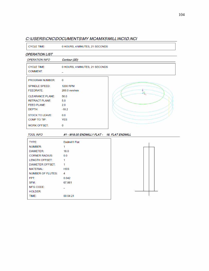
104

105

106
APPENDIX D
G CODE FOR CNC MACHINE
FOR BASE
%
O0000(BASE)
(DATE=DD-MM-YY - 23-05-16 TIME=HH:MM - 09:48)
(MCX FILE - F:\CNC MACHINING\BASE.MCX-5)
(NC FILE - F:\CNC MACHINING\BASE.NC)
(MATERIAL - ALUMINUM MM - 2024)
( T1 | 4. DRILL | H1 )
( T2 | 10.5 DRILL | H2 )
( T3 | 25 / 45 CHAMFER MILL | H3 )
( T4 | 12.00-1.75 TAP RH | H4 )
N100 G21
N102 G0 G17 G40 G49 G80 G90
N104 T1 M6
N106 G0 G90 G54 X-26.3 Y0. A0. S1000 M3
N108 G43 H1 Z1. M8
N110 G99 G83 Z-15. R1. Q.2 F50.
N112 X0. Y18.5
N114 X26.3 Y0.
N116 X0. Y-18.5
N118 G80
N120 M5
N122 G91 G28 Z0. M9
N124 A0.
N126 M01
N128 T2 M6
N130 G0 G90 G54 X0. Y0. A0. S700 M3
N132 G43 H2 Z1. M8
N134 G99 G83 Z-28. R1. Q.2 F50.
N136 G80
N138 M5
N140 G91 G28 Z0. M9
N142 A0.
N144 M01
N146 T3 M6
N148 G0 G90 G54 X0. Y0. A0. S500 M3
N150 G43 H3 Z1. M8
N152 G99 G81 Z-5. R1. F50.

107
N154 G80
N156 M5
N158 G91 G28 Z0. M9
N160 A0.
N162 M01
N164 T4 M6
N166 G0 G90 G54 X0. Y0. A0. S60 M3
N168 G43 H4 Z1. M8
N170 G99 G84 Z-25. R1. F105.
N172 G80
N174 M5
N176 G91 G28 Z0. M9
N178 G28 Y0. A0.
N180 M30
%
REPAIR BASE
%
O0000(BASE R)
(DATE=DD-MM-YY - 23-05-16 TIME=HH:MM - 10:50)
(MCX FILE - F:\CNC MACHINING\BASE.MCX-5)
(NC FILE - F:\CNC MACHINING\BASE R.NC)
(MATERIAL - ALUMINUM MM - 2024)
( T1 | 4. DRILL | H1 )
N100 G21
N102 G0 G17 G40 G49 G80 G90
N104 T1 M6
N106 G0 G90 G54 X0. Y18.5 A0. S1000 M3
N108 G43 H1 Z1. M8
N110 G99 G83 Z-28. R1. Q.2 F50.
N112 Y-18.5
N114 G80
N116 M5
N118 G91 G28 Z0. M9
N120 G28 Y0. A0.
N122 M30
%

108
FOR DIAPHRAGM
%
O0000(D)
(DATE=DD-MM-YY - 23-05-16 TIME=HH:MM - 11:21)
(MCX FILE - F:\CNC MACHINING\DIAPHRAGM.MCX-5)
(NC FILE - F:\CNC MACHINING\D.NC)
(MATERIAL - ALUMINUM MM - 2024)
( T1 | 18. FLAT ENDMILL | H1 )
( T2 | 2.6 DRILL | H2 )
( T3 | 25 / 45 CHAMFER MILL | H3 )
( T4 | 3.00-0.5 TAP RH | H4 )
N100 G21
N102 G0 G17 G40 G49 G80 G90
N104 T1 M6
N106 G0 G90 G54 X2.171 Y5.4 A0. S1200 M3
N108 G43 H1 Z5. M8
N110 Z2.
N112 G1 Z-.958 F50.
N114 X-.6 F200.
N116 G3 X-6. Y0. I0. J-5.4
N118 X0. Y-6. I6. J0.
N120 X6. Y0. I0. J6.
N122 X0. Y6. I-6. J0.
N124 X-6. Y0. I0. J-6.
N126 X-.6 Y-5.4 I5.4 J0.
N128 G1 X2.171
N130 G0 Z4.042
N132 Y5.4
N134 Z1.042
N136 G1 Z-1.916 F50.
N138 X-.6 F200.
N140 G3 X-6. Y0. I0. J-5.4
N142 X0. Y-6. I6. J0.
N144 X6. Y0. I0. J6.
N146 X0. Y6. I-6. J0.
N148 X-6. Y0. I0. J-6.
N150 X-.6 Y-5.4 I5.4 J0.
N152 G1 X2.171
N154 G0 Z3.084
N156 Y5.4
N158 Z.084
N160 G1 Z-2.874 F50.

109
N162 X-.6 F200.
N164 G3 X-6. Y0. I0. J-5.4
N166 X0. Y-6. I6. J0.
N168 X6. Y0. I0. J6.
N170 X0. Y6. I-6. J0.
N172 X-6. Y0. I0. J-6.
N174 X-.6 Y-5.4 I5.4 J0.
N176 G1 X2.171
N178 G0 Z2.126
N180 Y5.4
N182 Z-.874
N184 G1 Z-3.832 F50.
N186 X-.6 F200.
N188 G3 X-6. Y0. I0. J-5.4
N190 X0. Y-6. I6. J0.
N192 X6. Y0. I0. J6.
N194 X0. Y6. I-6. J0.
N196 X-6. Y0. I0. J-6.
N198 X-.6 Y-5.4 I5.4 J0.
N200 G1 X2.171
N202 G0 Z1.168
N204 Y5.4
N206 Z-1.832
N208 G1 Z-4.789 F50.
N210 X-.6 F200.
N212 G3 X-6. Y0. I0. J-5.4
N214 X0. Y-6. I6. J0.
N216 X6. Y0. I0. J6.
N218 X0. Y6. I-6. J0.
N220 X-6. Y0. I0. J-6.
N222 X-.6 Y-5.4 I5.4 J0.
N224 G1 X2.171
N226 G0 Z.211
N228 Y5.4
N230 Z-2.789
N232 G1 Z-5.747 F50.
N234 X-.6 F200.
N236 G3 X-6. Y0. I0. J-5.4
N238 X0. Y-6. I6. J0.
N240 X6. Y0. I0. J6.
N242 X0. Y6. I-6. J0.
N244 X-6. Y0. I0. J-6.
N246 X-.6 Y-5.4 I5.4 J0.

110
N248 G1 X2.171
N250 G0 Z-.747
N252 Y5.4
N254 Z-3.747
N256 G1 Z-6.705 F50.
N258 X-.6 F200.
N260 G3 X-6. Y0. I0. J-5.4
N262 X0. Y-6. I6. J0.
N264 X6. Y0. I0. J6.
N266 X0. Y6. I-6. J0.
N268 X-6. Y0. I0. J-6.
N270 X-.6 Y-5.4 I5.4 J0.
N272 G1 X2.171
N274 G0 Z-1.705
N276 Y5.4
N278 Z-4.705
N280 G1 Z-7.663 F50.
N282 X-.6 F200.
N284 G3 X-6. Y0. I0. J-5.4
N286 X0. Y-6. I6. J0.
N288 X6. Y0. I0. J6.
N290 X0. Y6. I-6. J0.
N292 X-6. Y0. I0. J-6.
N294 X-.6 Y-5.4 I5.4 J0.
N296 G1 X2.171
N298 G0 Z-2.663
N300 Y5.4
N302 Z-5.663
N304 G1 Z-8.621 F50.
N306 X-.6 F200.
N308 G3 X-6. Y0. I0. J-5.4
N310 X0. Y-6. I6. J0.
N312 X6. Y0. I0. J6.
N314 X0. Y6. I-6. J0.
N316 X-6. Y0. I0. J-6.
N318 X-.6 Y-5.4 I5.4 J0.
N320 G1 X2.171
N322 G0 Z-3.621
N324 Y5.4
N326 Z-6.621
N328 G1 Z-9.579 F50.
N330 X-.6 F200.
N332 G3 X-6. Y0. I0. J-5.4

111
N334 X0. Y-6. I6. J0.
N336 X6. Y0. I0. J6.
N338 X0. Y6. I-6. J0.
N340 X-6. Y0. I0. J-6.
N342 X-.6 Y-5.4 I5.4 J0.
N344 G1 X2.171
N346 G0 Z-4.579
N348 Y5.4
N350 Z-7.579
N352 G1 Z-10.537 F50.
N354 X-.6 F200.
N356 G3 X-6. Y0. I0. J-5.4
N358 X0. Y-6. I6. J0.
N360 X6. Y0. I0. J6.
N362 X0. Y6. I-6. J0.
N364 X-6. Y0. I0. J-6.
N366 X-.6 Y-5.4 I5.4 J0.
N368 G1 X2.171
N370 G0 Z-5.537
N372 Y5.4
N374 Z-8.537
N376 G1 Z-11.495 F50.
N378 X-.6 F200.
N380 G3 X-6. Y0. I0. J-5.4
N382 X0. Y-6. I6. J0.
N384 X6. Y0. I0. J6.
N386 X0. Y6. I-6. J0.
N388 X-6. Y0. I0. J-6.
N390 X-.6 Y-5.4 I5.4 J0.
N392 G1 X2.171
N394 G0 Z-6.495
N396 Y5.4
N398 Z-9.495
N400 G1 Z-12.453 F50.
N402 X-.6 F200.
N404 G3 X-6. Y0. I0. J-5.4
N406 X0. Y-6. I6. J0.
N408 X6. Y0. I0. J6.
N410 X0. Y6. I-6. J0.
N412 X-6. Y0. I0. J-6.
N414 X-.6 Y-5.4 I5.4 J0.
N416 G1 X2.171
N418 G0 Z-7.453

112
N420 Y5.4
N422 Z-10.453
N424 G1 Z-13.411 F50.
N426 X-.6 F200.
N428 G3 X-6. Y0. I0. J-5.4
N430 X0. Y-6. I6. J0.
N432 X6. Y0. I0. J6.
N434 X0. Y6. I-6. J0.
N436 X-6. Y0. I0. J-6.
N438 X-.6 Y-5.4 I5.4 J0.
N440 G1 X2.171
N442 G0 Z-8.411
N444 Y5.4
N446 Z-11.411
N448 G1 Z-14.368 F50.
N450 X-.6 F200.
N452 G3 X-6. Y0. I0. J-5.4
N454 X0. Y-6. I6. J0.
N456 X6. Y0. I0. J6.
N458 X0. Y6. I-6. J0.
N460 X-6. Y0. I0. J-6.
N462 X-.6 Y-5.4 I5.4 J0.
N464 G1 X2.171
N466 G0 Z-9.368
N468 Y5.4
N470 Z-12.368
N472 G1 Z-15.326 F50.
N474 X-.6 F200.
N476 G3 X-6. Y0. I0. J-5.4
N478 X0. Y-6. I6. J0.
N480 X6. Y0. I0. J6.
N482 X0. Y6. I-6. J0.
N484 X-6. Y0. I0. J-6.
N486 X-.6 Y-5.4 I5.4 J0.
N488 G1 X2.171
N490 G0 Z-10.326
N492 Y5.4
N494 Z-13.326
N496 G1 Z-16.284 F50.
N498 X-.6 F200.
N500 G3 X-6. Y0. I0. J-5.4
N502 X0. Y-6. I6. J0.
N504 X6. Y0. I0. J6.

113
N506 X0. Y6. I-6. J0.
N508 X-6. Y0. I0. J-6.
N510 X-.6 Y-5.4 I5.4 J0.
N512 G1 X2.171
N514 G0 Z-11.284
N516 Y5.4
N518 Z-14.284
N520 G1 Z-17.242 F50.
N522 X-.6 F200.
N524 G3 X-6. Y0. I0. J-5.4
N526 X0. Y-6. I6. J0.
N528 X6. Y0. I0. J6.
N530 X0. Y6. I-6. J0.
N532 X-6. Y0. I0. J-6.
N534 X-.6 Y-5.4 I5.4 J0.
N536 G1 X2.171
N538 G0 Z-12.242
N540 Y5.4
N542 Z-15.242
N544 G1 Z-18.2 F50.
N546 X-.6 F200.
N548 G3 X-6. Y0. I0. J-5.4
N550 X0. Y-6. I6. J0.
N552 X6. Y0. I0. J6.
N554 X0. Y6. I-6. J0.
N556 X-6. Y0. I0. J-6.
N558 X-.6 Y-5.4 I5.4 J0.
N560 G1 X2.171
N562 G0 Z5.
N564 M5
N566 G91 G28 Z0. M9
N568 A0.
N570 M01
N572 T2 M6
N574 G0 G90 G54 X-19. Y0. A0. S1000 M3
N576 G43 H2 Z1. M8
N578 G99 G83 Z-17.5 R1. Q.1 F30.
N580 X19.
N582 G80
N584 M5
N586 G91 G28 Z0. M9
N588 A0.
N590 M01
114
N592 T3 M6
N594 G0 G90 G54 X-19. Y0. A0. S600 M3
N596 G43 H3 Z1. M8
N598 G99 G82 Z-1.5 R1. P.5 F50.
N600 X19.
N602 G80
N604 M5
N606 G91 G28 Z0. M9
N608 A0.
N610 M01
N612 T4 M6
N614 G0 G90 G54 X-19. Y0. A0. S90 M3
N616 G43 H4 Z1. M8
N618 G99 G84 Z-11. R1. F45.
N620 X19.
N622 G80
N624 M5
N626 G91 G28 Z0. M9
N628 G28 Y0. A0.
N630 M30
%

115
APPENDIX F
LIST OF MATERIAL AND EQUIPMENT
. Table 3.2 below shows the list of material and equipment used to design the fiber Bragg
grating pressure transducer shown with a picture and are indicated
Table 3.2: List of Material and Equipment
Parts Material Picture Specification Quantity
1 Aluminum
Rod
10cm with 6cm
diameter
1
2 Screws
4
3 Fiber Bragg
grating
Sensor
1546.767nm
2
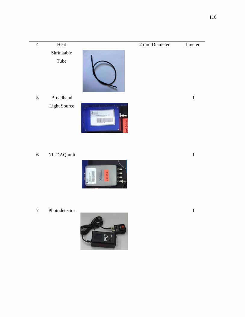
116
4 Heat
Shrinkable
Tube
2 mm Diameter 1 meter
5 Broadband
Light Source
1
6 NI- DAQ unit
1
7 Photodetector
1
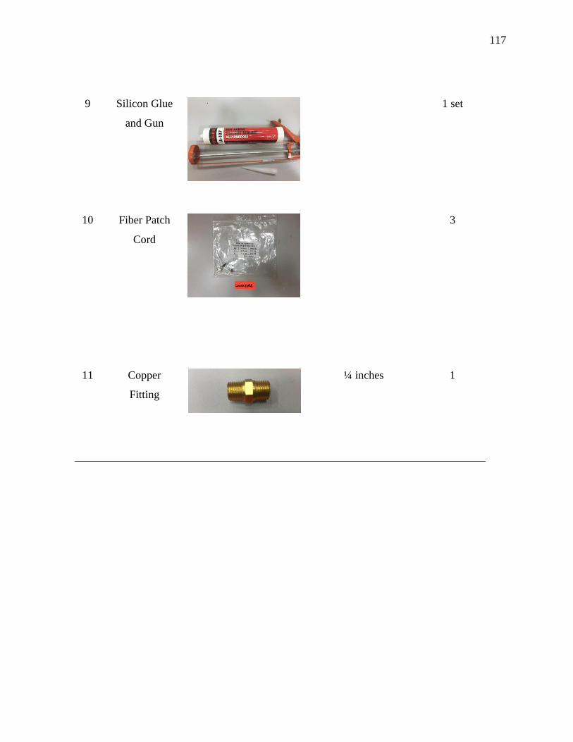
117
9 Silicon Glue
and Gun
1 set
10 Fiber Patch
Cord
3
11 Copper
Fitting
¼ inches 1

118
APPENDIX G
MATLAB CODING FOR NORMALIZATION OF VOLTAGE
function varargout = untitled(varargin)
% UNTITLED MATLAB code for untitled.fig
% UNTITLED, by itself, creates a new UNTITLED or raises the existing
% singleton*.
%
% H = UNTITLED returns the handle to a new UNTITLED or the handle to
% the existing singleton*.
%
% UNTITLED('CALLBACK',hObject,eventData,handles,...) calls the local
% function named CALLBACK in UNTITLED.M with the given input arguments.
%
% UNTITLED('Property','Value',...) creates a new UNTITLED or raises the
% existing singleton*. Starting from the left, property value pairs are
% applied to the GUI before untitled_OpeningFcn gets called. An
% unrecognized property name or invalid value makes property application
% stop. All inputs are passed to untitled_OpeningFcn via varargin.
%
% *See GUI Options on GUIDE's Tools menu. Choose "GUI allows only one
% instance to run (singleton)".
%
% See also: GUIDE, GUIDATA, GUIHANDLES
% Edit the above text to modify the response to help untitled
% Last Modified by GUIDE v2.5 01-Jun-2016 16:58:11
% Begin initialization code - DO NOT EDIT
gui_Singleton = 1;
gui_State = struct('gui_Name', mfilename, ...
'gui_Singleton', gui_Singleton, ...
'gui_OpeningFcn', @untitled_OpeningFcn, ...
'gui_OutputFcn', @untitled_OutputFcn, ...
'gui_LayoutFcn', [] , ...
'gui_Callback', []);
if nargin && ischar(varargin{1})
gui_State.gui_Callback = str2func(varargin{1});
end
if nargout

119
[varargout{1:nargout}] = gui_mainfcn(gui_State, varargin{:});
else
gui_mainfcn(gui_State, varargin{:});
end
% End initialization code - DO NOT EDIT
% --- Executes just before untitled is made visible.
function untitled_OpeningFcn(hObject, eventdata, handles, varargin)
% This function has no output args, see OutputFcn.
% hObject handle to figure
% eventdata reserved - to be defined in a future version of MATLAB
% handles structure with handles and user data (see GUIDATA)
% varargin command line arguments to untitled (see VARARGIN)
% Choose default command line output for untitled
handles.output = hObject;
% Update handles structure
guidata(hObject, handles);
% UIWAIT makes untitled wait for user response (see UIRESUME)
% uiwait(handles.figure1);
% --- Outputs from this function are returned to the command line.
function varargout = untitled_OutputFcn(hObject, eventdata, handles)
% varargout cell array for returning output args (see VARARGOUT);
% hObject handle to figure
% eventdata reserved - to be defined in a future version of MATLAB
% handles structure with handles and user data (see GUIDATA)
% Get default command line output from handles structure
varargout{1} = handles.output;
axes(handles.axes1);
imshow('Aurora.jpg');
axes(handles.axes4);
imshow('UMP.jpeg');
t=datestr(clock,'dd-mm-yy HH:MM:SS');
set(handles.text10,'String',t,'FontSize',11);
% creating the timer object, so that live mode is possible
timer_obj = timer(...
'StartFcn', @user_timer_start, ... % start function
120
'TimerFcn', {@user_timer_update, hObject}, ... % timer function, has to specific the
handle to the GUI,
'StopFcn', @user_timer_stop, ... % stop function
'ErrorFcn', @user_timer_err, ... % error function
'ExecutionMode', 'fixedRate', ... %
'Period', 0.1, ... % updates every xx seconds
'TasksToExecute', inf, ...
'BusyMode', 'drop');
% save the timer object as application data
setappdata(hObject, 'timer_obj', timer_obj); % need to save it because we need to stop
and delete it when quit
start(timer_obj);
% UIWAIT makes myClock wait for user response (see UIRESUME)
% uiwait(handles.figure1);
% --- Outputs from this function are returned to the command line.
function varargout = myClock_OutputFcn(hObject, eventdata, handles)
% varargout cell array for returning output args (see VARARGOUT);
% hObject handle to figure
% eventdata reserved - to be defined in a future version of MATLAB
% handles structure with handles and user data (see GUIDATA)
% Get default command line output from handles structure
varargout{1} = handles.output;
function user_timer_update(src,evt, fig_handle)
handles = guihandles(fig_handle);
set(handles.text11, 'string', datestr(now, 'dd-mm-yy HH:MM:SS'),'FontSize',11);
function user_timer_start(src, evt)
disp('Timer started!');
function user_timer_stop(src, evt)
disp('Timer stop');
121
function user_timer_err(src, evt)
disp('Timer error');
% --- Executes when user attempts to close figure1.
function figure1_CloseRequestFcn(hObject, eventdata, handles)
% hObject handle to figure1 (see GCBO)
% eventdata reserved - to be defined in a future version of MATLAB
% handles structure with handles and user data (see GUIDATA)
% Hint: delete(hObject) closes the figure
stop(getappdata(hObject, 'timer_obj'));
delete(getappdata(hObject, 'timer_obj'));
delete(hObject);
% --- Executes on button press in pushbutton2.
function pushbutton2_Callback(hObject, eventdata, handles)
% hObject handon2 (see GCBO)
% eventdata reserved - to be defined in a future verle to pushbuttsion of MATLAB
% handles structure with handles and user data (see GUIDATA)
ID=get(handles.edit2,'String');
Channel=get(handles.edit3,'String');
s=daq.createSession('ni');
s.Rate=256000;
s.addAnalogInputChannel(ID,Channel,'Voltage');
k=0;
i=1;
n=0;
while k<100
[data,time]=s.startForeground;
axes(handles.axes5);
plot(data);
set(get(handles.axes5, 'XLabel'), 'String', 'Time (seconds)');
set(get(handles.axes5, 'YLabel'), 'String', 'Voltage (V)');
set(get(handles.axes5, 'Title'), 'String', 'Voltage vs Time');
p=mean(data);
set(handles.text12,'String',p,'FontSize',13);
if k<1;
set(handles.text19,'string',p,'FontSize',13);
end
a=str2double(get(handles.text19,'String'));

122
k=p/a;
set(handles.text18,'String',k,'FontSize',16);
y=(((k-0.9954)/-0.0581)*100)-1.325;
set(handles.text13,'String',y,'FontSize',33);
if(n <=100)
b(i)=y ;
i=i+1;
set(gcf,'color','white');
drawnow;
axes(handles.axes8);
plot(b,'-.dk','linewidth',1.8), axis([1 100 -100 300])
grid on;
title('Record')
xlabel('Time(s)');
ylabel('Pressure(kPa)');
n = n + 1;
pause(1.0);
end
%filename = 'testdata.xlsx';
%A = [y];
%xlswrite(filename,A)
k=k+1;
end
% --- Executes on button press in pushbutton3.
function pushbutton3_Callback(hObject, eventdata, handles)
% hObject handle to pushbutton3 (see GCBO)
% eventdata reserved - to be defined in a future version of MATLAB
% handles structure with handles and user data (see GUIDATA)
cl = questdlg('Do you want to EXIT?','EXIT',...
'Yes','No','No');
switch cl
case 'Yes'
close();
clear all;
return;
case 'No'
quit cancel;
end
% --- Executes on button press in pushbutton4.
function pushbutton4_Callback(hObject, eventdata, handles)

123
% hObject handle to pushbutton4 (see GCBO)
% eventdata reserved - to be defined in a future version of MATLAB
% handles structure with handles and user data (see GUIDATA)
hdaq=daq.getDevices;
if~isempty(hdaq)
msgbox(sprintf('%s Device Located',hdaq.Description),'Modal')
hdaq
handles.hdaq = hdaq;
set(handles.edit2,'string',hdaq.ID)
else
errordlg('No DAQ Device Found.')
set(handles.edit2,'string','No Device Found')
end
guidata(hObject,handles)
function edit2_Callback(hObject, eventdata, handles)
% hObject handle to edit2 (see GCBO)
% eventdata reserved - to be defined in a future version of MATLAB
% handles structure with handles and user data (see GUIDATA)
% Hints: get(hObject,'String') returns contents of edit2 as text
% str2double(get(hObject,'String')) returns contents of edit2 as a double
% --- Executes during object creation, after setting all properties.
function edit2_CreateFcn(hObject, eventdata, handles)
% hObject handle to edit2 (see GCBO)
% eventdata reserved - to be defined in a future version of MATLAB
% handles empty - handles not created until after all CreateFcns called
% Hint: edit controls usually have a white background on Windows.
% See ISPC and COMPUTER.
if ispc && isequal(get(hObject,'BackgroundColor'), get(0,'defaultUicontrolBackgroundColor'))
set(hObject,'BackgroundColor','white');
end
function edit3_Callback(hObject, eventdata, handles)

124
% hObject handle to edit3 (see GCBO)
% eventdata reserved - to be defined in a future version of MATLAB
% handles structure with handles and user data (see GUIDATA)
% Hints: get(hObject,'String') returns contents of edit3 as text
% str2double(get(hObject,'String')) returns contents of edit3 as a double
% --- Executes during object creation, after setting all properties.
function edit3_CreateFcn(hObject, eventdata, handles)
% hObject handle to edit3 (see GCBO)
% eventdata reserved - to be defined in a future version of MATLAB
% handles empty - handles not created until after all CreateFcns called
% Hint: edit controls usually have a white background on Windows.
% See ISPC and COMPUTER.
if ispc && isequal(get(hObject,'BackgroundColor'), get(0,'defaultUicontrolBackgroundColor'))
set(hObject,'BackgroundColor','white');
end
% --- Executes on button press in pushbutton5.
function pushbutton5_Callback(hObject, eventdata, handles)
% hObject handle to pushbutton5 (see GCBO)
% eventdata reserved - to be defined in a future version of MATLAB
% handles structure with handles and user data (see GUIDATA)
screenshot = getframe(gcf);
[jpegfile, path2jpeg] = uiputfile('.jpeg');
FileName = fullfile(path2jpeg, jpegfile);
imwrite (screenshot.cdata, FileName, 'jpg');
% --- Executes on button press in pushbutton6.
function pushbutton6_Callback(hObject, eventdata, handles)
% hObject handle to pushbutton6 (see GCBO)
% eventdata reserved - to be defined in a future version of MATLAB
% handles structure with handles and user data (see GUIDATA)
uiresume(gcbf)
% --- Executes on button press in pushbutton7.
function pushbutton7_Callback(hObject, eventdata, handles)
% hObject handle to pushbutton7 (see GCBO)
% eventdata reserved - to be defined in a future version of MATLAB

125
% handles structure with handles and user data (see GUIDATA)
uiwait(gcbf)
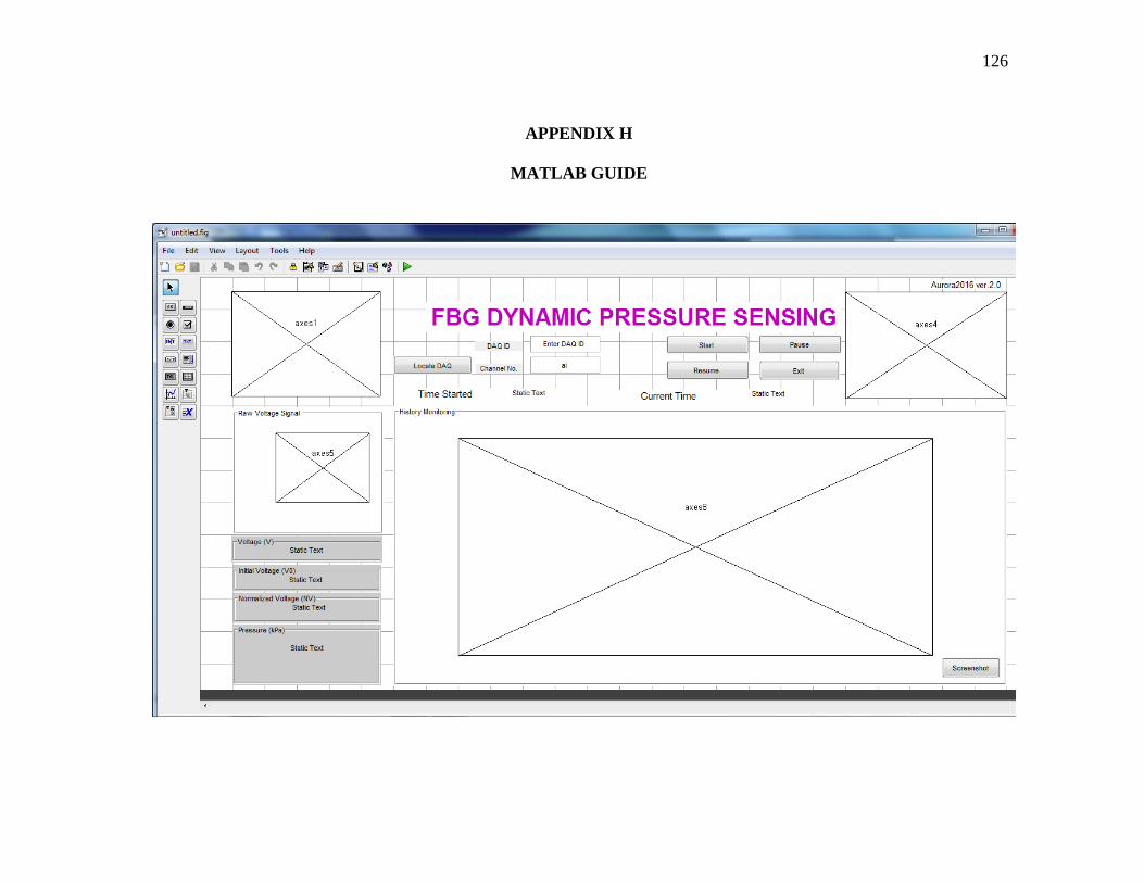
126
APPENDIX H
MATLAB GUIDE
Recommended