Thermal Conductivity of Trinidad ‘Guanapo Sharp Sand’
Krishpersad Manohar, Lecturer, Mechanical and Manufacturing Engineering Department, The University of the West Indies, St. Augustine, Trinidad, West
Indies. Email: [email protected] Kimberly Ramroop, M.Phil. Candidate, Mechanical and Manufacturing
Engineering Department, The University of the West Indies, St. Augustine, Trinidad, West Indies.
Gurmohan S. Kochhar, Professor, Department of Mechanical & Manufacturing Engineering, The University of the West Indies, St. Augustine, Trinidad, West
Indies. Email: [email protected]
ABSTRACT
The thermal conductivity variation of “sharp sand” with moisture and grain size
was investigated using a thermal probe method. The probe used for testing was
built in accordance with ASTM D 5334 and calibrated using heat-flow meter data.
Calibration tests demonstrated repeatability ± 3.5% for a 95% confidence of the
dT/ d ln t slope. Experiments were conducted on two sand specimens with grain
size ranging from 150µm to 300µm (fine) and 301µm to 600µm (coarse). Test
density was maintained at approximately 1400 kg/m3 for each specimen and data
were recorded for specimens with 0%, 2.5%, 5% and 7.5% wt.% water. The
experimental results showed a well defined increase in λ with water content for
both specimens. The fine sand has a more rapid increase in λ with water content
then the coarse sand.
NOMENCLATURE
n Number of data points in chosen time interval
Q Power emitted by probe per unit length (W/m)
R Electrical resistance (Ω)
r Radial distance from probe (mm)
T Temperature (oC)
To Initial temperature (oC)
t Time (s)
V Voltage (V)
V Volume (m3)
W Weight (kg)
κ Thermal diffusivity (m2/s)
λ Apparent thermal conductivity (W/m.K)
1. INTRODUCTION
Sand and granular material are commonly used as protective shock-absorbing
material around pipelines and underground cables. A layer of backfill granular
material gives stability and serves as a protection by allowing for some movement.
In many cases, however, the thermal properties of the material are of significant
importance as electrical cables need to dissipate the internally generated heat and
gas and steam lines may be affected by the heat gain or loss from the surroundings.
The thermal characteristics of the backfill material and the variation with
moisture will determine the extent of the thermal influence. The thermal properties
of granular material are influenced by the water content, pore space and packing
density. Compared to air, water has a high thermal conductivity, hence, a small
amount of distributed water will significantly affect the thermal conductivity. Grain
size and packing density have an effect on the solid-phase conduction.
2. SAND TYPE
The material selected for this study was Guanapo Sand, locally known as ‘sharp
sand’. This material is readily available at the Turure National Quarries Plant,
Trinidad, West Indies, and is found as terrace deposits and river gravel in the
northern basin of Trinidad. Guanapo Sand is a well-characterized material with a
slight yellow color that consists of 98% silica and traces of iron oxide.
From randomly selected samples, two different grain size range were obtained.
A mechanical shaker was used to separate particles passing a 300 µm sieve but
retained on a 150 µm sieve defined the fine sand specimen. This material is
described as a fine sand with sub-angular and sub-rounded grains. Particles passing
a 600 µm sieve but retained on a 300 µm sieve made up the coarser grain specimen.
This material is described as medium sand with sub-angular and sub-rounded grains
[1].
3. SPECIMEN CONDITIONING
The graded sand samples were dried in a dehumidifying chamber at 50oC to
avoid any micro-structural changes. Test specimens were weighed at 24 h intervals
until no change in weight was observed. This condition was taken as zero percent
water content and used as the datum for wt.% water.
4. TEST SPECIMEN SIZING
From the theory of the continuous line source heater [2, 3], Equation 1 is the
approximate solution for the temperature variation with time in an infinite solid,
initially at temperature To, heated by a line source.
T - To = (Q/4πκ)ln(4κt/r2) – 0.5772(Q/4πκ) (1)
Using a specific heat and thermal conductivity estimate of 0.796 kJ/kg.K and 2
W/m.K, respectively, for a density of 1400 kg/m3 [4, 5], the radial distance r at
which T – To is zero after 1000 s was calculated to be 65 mm. Therefore, for all
practical purposes, cylindrical specimens of radius 150 mm radius represented an
infinite medium with respect to a line source heater over a test time of 1000 s.
5. SAMPLE PREPARATION
Sand specimens 200 mm deep were used to ensure that when the 100 mm probe
was fully inserted to represent the line source, end effects would be negligible. The
weight, W, of dry sand for each specimen was calculated from the volume, V, of the
sand in cubic meters.
W = V x 1400 (2)
For the dry sand specimens the weighed sand was uniformly packed in the
cylindrical container to the 200 mm height to produce the approximate target
density of 1400 kg/m3.
For the wet sand specimens, the respective mass of dry sand was mixed with the
mass of water required to give the necessary moisture content. The water and sand
were mixed manually to form a homogeneous mixture. Test specimens were re-
weighed after mixing to ensure the correct water content. The wet sand was then
packed into the cylindrical test containers to the required depth such that a density
of 1400 kg/m3 was achieved. For each grain size five test specimens were prepared
with 0, 2.5, 5.0 and 7.5 wt.% water. For 10 wt.% water the test specimens drained
off excess water showing that the sand was water saturated between 7.5 to 10 wt.%
water.
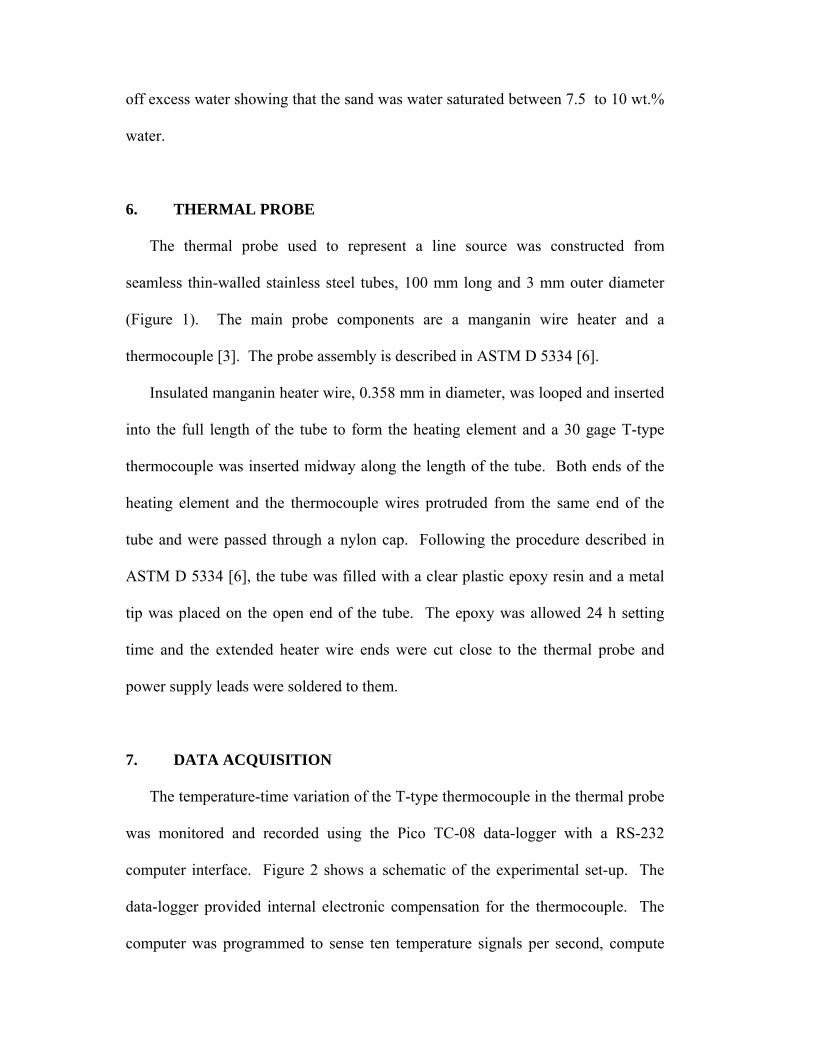
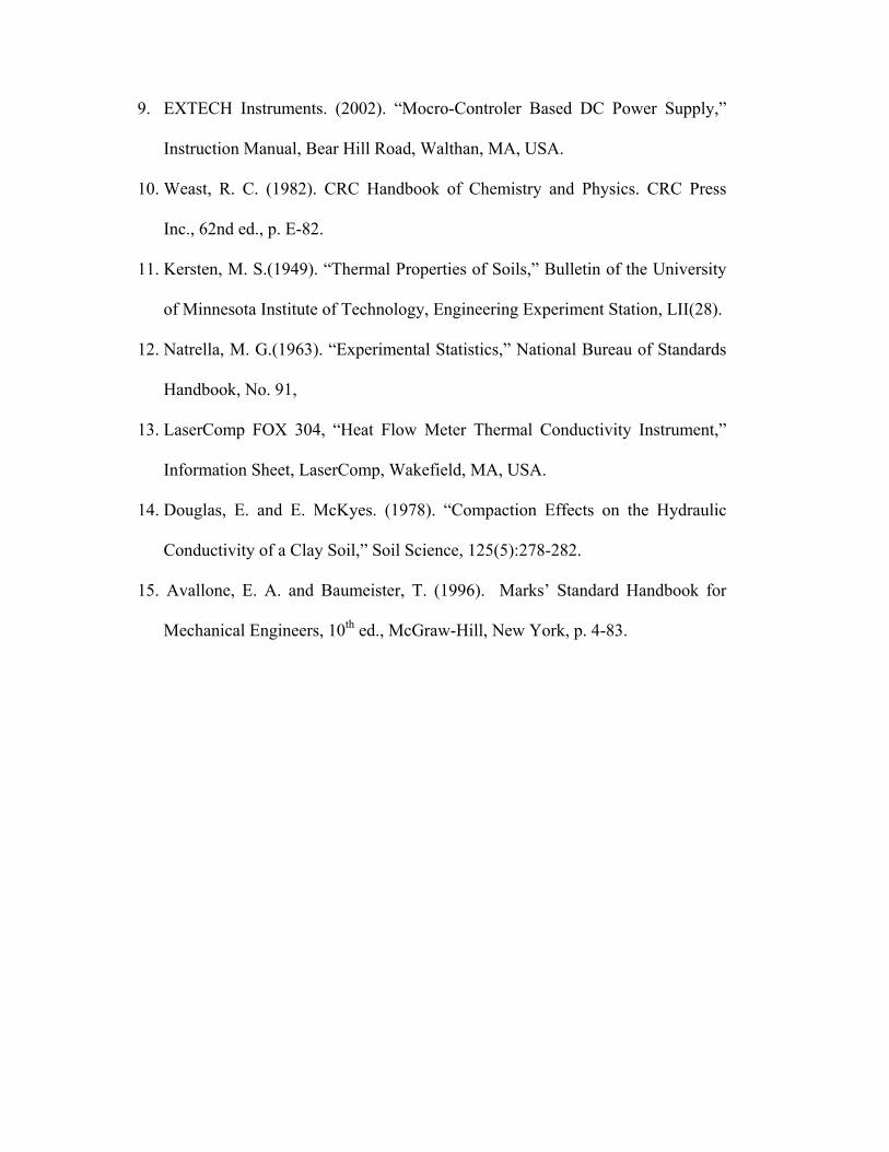
6. THERMAL PROBE
The thermal probe used to represent a line source was constructed from
seamless thin-walled stainless steel tubes, 100 mm long and 3 mm outer diameter
(Figure 1). The main probe components are a manganin wire heater and a
thermocouple [3]. The probe assembly is described in ASTM D 5334 [6].
Insulated manganin heater wire, 0.358 mm in diameter, was looped and inserted
into the full length of the tube to form the heating element and a 30 gage T-type
thermocouple was inserted midway along the length of the tube. Both ends of the
heating element and the thermocouple wires protruded from the same end of the
tube and were passed through a nylon cap. Following the procedure described in
ASTM D 5334 [6], the tube was filled with a clear plastic epoxy resin and a metal
tip was placed on the open end of the tube. The epoxy was allowed 24 h setting
time and the extended heater wire ends were cut close to the thermal probe and
power supply leads were soldered to them.
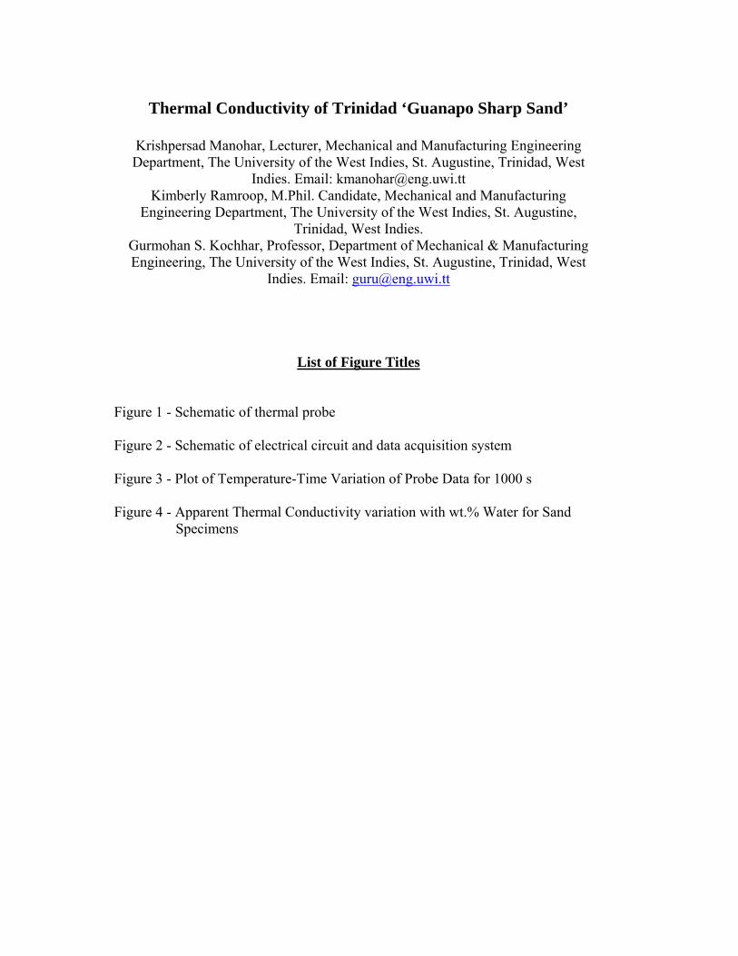
7. DATA ACQUISITION
The temperature-time variation of the T-type thermocouple in the thermal probe
was monitored and recorded using the Pico TC-08 data-logger with a RS-232
computer interface. Figure 2 shows a schematic of the experimental set-up. The
data-logger provided internal electronic compensation for the thermocouple. The
computer was programmed to sense ten temperature signals per second, compute
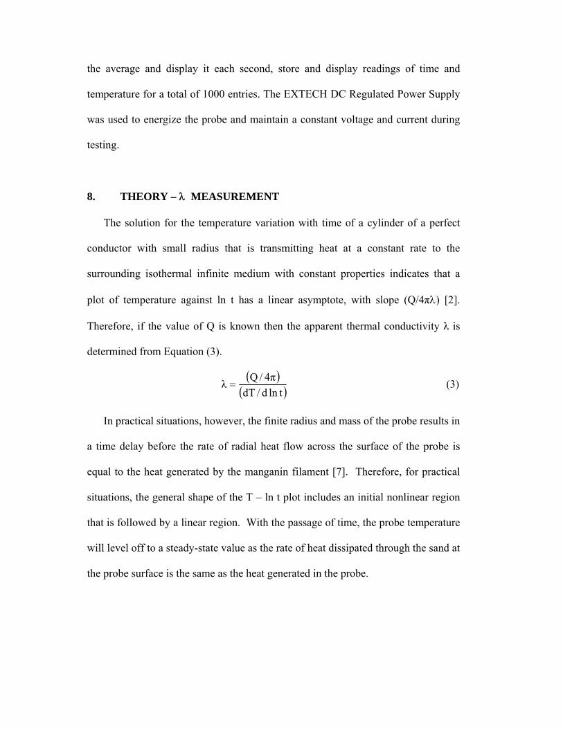
the average and display it each second, store and display readings of time and
temperature for a total of 1000 entries. The EXTECH DC Regulated Power Supply
was used to energize the probe and maintain a constant voltage and current during
testing.
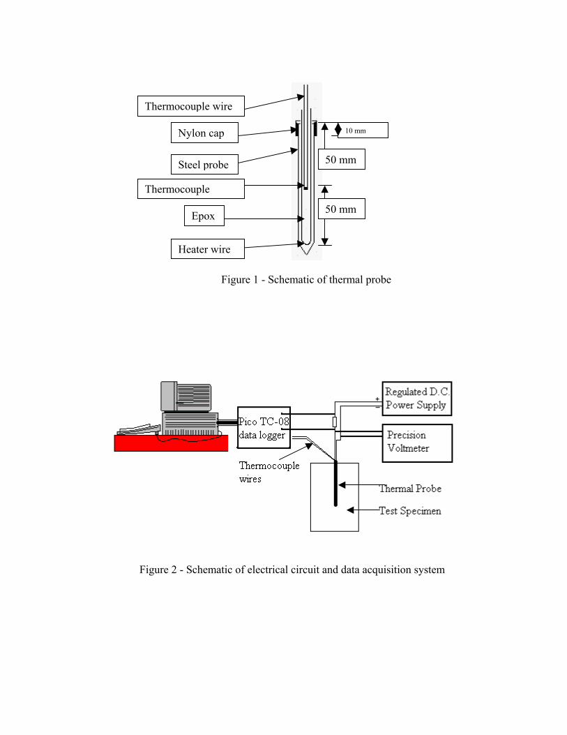
8. THEORY – λ MEASUREMENT
The solution for the temperature variation with time of a cylinder of a perfect
conductor with small radius that is transmitting heat at a constant rate to the
surrounding isothermal infinite medium with constant properties indicates that a
plot of temperature against ln t has a linear asymptote, with slope (Q/4πλ) [2].
Therefore, if the value of Q is known then the apparent thermal conductivity λ is
determined from Equation (3).
( )( )tlnd/dT
4π/Qλ = (3)
In practical situations, however, the finite radius and mass of the probe results in
a time delay before the rate of radial heat flow across the surface of the probe is
equal to the heat generated by the manganin filament [7]. Therefore, for practical
situations, the general shape of the T – ln t plot includes an initial nonlinear region
that is followed by a linear region. With the passage of time, the probe temperature
will level off to a steady-state value as the rate of heat dissipated through the sand at
the probe surface is the same as the heat generated in the probe.
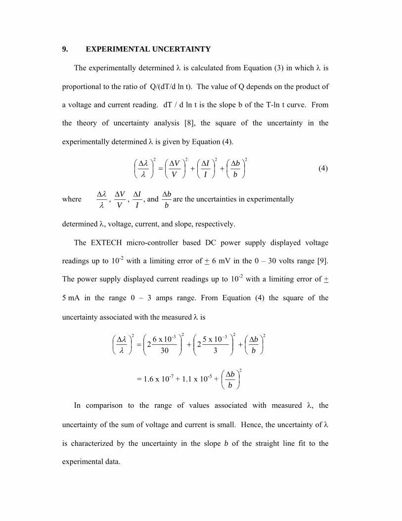
9. EXPERIMENTAL UNCERTAINTY
The experimentally determined λ is calculated from Equation (3) in which λ is
proportional to the ratio of Q/(dT/d ln t). The value of Q depends on the product of
a voltage and current reading. dT / d ln t is the slope b of the T-ln t curve. From
the theory of uncertainty analysis [8], the square of the uncertainty in the
experimentally determined λ is given by Equation (4).
2222
⎟⎠⎞
⎜⎝⎛ ∆
+⎟⎠⎞
⎜⎝⎛ ∆
+⎟⎠⎞
⎜⎝⎛ ∆
=⎟⎠⎞
⎜⎝⎛ ∆
bb
II
VV
λλ (4)
where λλ∆ ,
VV∆ ,
II∆ , and
bb∆ are the uncertainties in experimentally
determined λ, voltage, current, and slope, respectively.
The EXTECH micro-controller based DC power supply displayed voltage
readings up to 10-2 with a limiting error of + 6 mV in the 0 – 30 volts range [9].
The power supply displayed current readings up to 10-2 with a limiting error of +
5 mA in the range 0 – 3 amps range. From Equation (4) the square of the
uncertainty associated with the measured λ is
2232-32
310x52
3010x 62 ⎟
⎠⎞
⎜⎝⎛ ∆
+⎟⎟⎠
⎞⎜⎜⎝
⎛+⎟⎟
⎠
⎞⎜⎜⎝
⎛=⎟
⎠⎞
⎜⎝⎛ ∆ −
bb
λλ
= 1.6 x 10⁻⁷ + 1.1 x 10⁻⁵ + 2
⎟⎠⎞
⎜⎝⎛ ∆
bb
In comparison to the range of values associated with measured λ, the
uncertainty of the sum of voltage and current is small. Hence, the uncertainty of λ
is characterized by the uncertainty in the slope b of the straight line fit to the
experimental data.
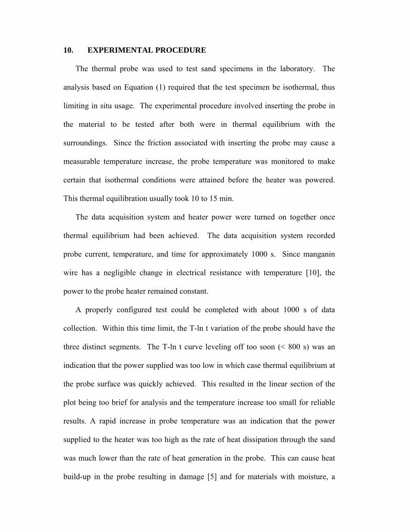
10. EXPERIMENTAL PROCEDURE
The thermal probe was used to test sand specimens in the laboratory. The
analysis based on Equation (1) required that the test specimen be isothermal, thus
limiting in situ usage. The experimental procedure involved inserting the probe in
the material to be tested after both were in thermal equilibrium with the
surroundings. Since the friction associated with inserting the probe may cause a
measurable temperature increase, the probe temperature was monitored to make
certain that isothermal conditions were attained before the heater was powered.
This thermal equilibration usually took 10 to 15 min.
The data acquisition system and heater power were turned on together once
thermal equilibrium had been achieved. The data acquisition system recorded
probe current, temperature, and time for approximately 1000 s. Since manganin
wire has a negligible change in electrical resistance with temperature [10], the
power to the probe heater remained constant.
A properly configured test could be completed with about 1000 s of data
collection. Within this time limit, the T-ln t variation of the probe should have the
three distinct segments. The T-ln t curve leveling off too soon (< 800 s) was an
indication that the power supplied was too low in which case thermal equilibrium at
the probe surface was quickly achieved. This resulted in the linear section of the
plot being too brief for analysis and the temperature increase too small for reliable
results. A rapid increase in probe temperature was an indication that the power
supplied to the heater was too high as the rate of heat dissipation through the sand
was much lower than the rate of heat generation in the probe. This can cause heat
build-up in the probe resulting in damage [5] and for materials with moisture, a
large rapid temperature gradient could result in moisture vaporization, causing a
change in material properties [11]. The power was adjusted up or down to satisfy
the test design time of 1000 s as recommended by ASTM D 5334 [6].
11. TEST DESIGN CRITERIA
The theory associated with determining apparent thermal conductivity from the
T-ln t plot of the thermal probe (Equation 3) makes use of the slope associated with
the linear segment of the heat-up curve. A least-square fit to a linear expression for
T in terms of ln t was used to describe this segment of the heat-up curve. The
analysis involves determining the slope for candidate intervals of 0 to 1000 s, 50 to
950 s, 100 to 900 s etc. The linear segment was taken to be such that three
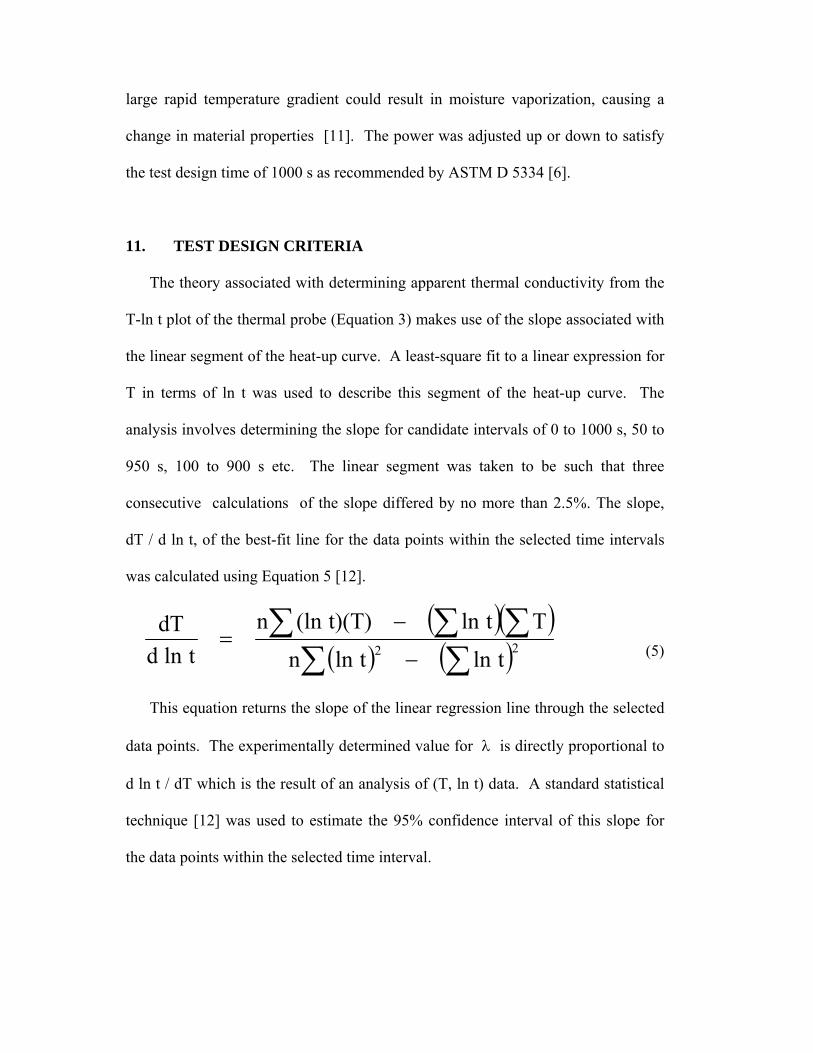
consecutive calculations of the slope differed by no more than 2.5%. The slope,
dT / d ln t, of the best-fit line for the data points within the selected time intervals
was calculated using Equation 5 [12].
( )( )( ) ( )∑ ∑
∑ ∑∑−
−= 22 tlntlnn
Ttlnt)(T)(lnntlnd
dT (5)
This equation returns the slope of the linear regression line through the selected
data points. The experimentally determined value for λ is directly proportional to
d ln t / dT which is the result of an analysis of (T, ln t) data. A standard statistical
technique [12] was used to estimate the 95% confidence interval of this slope for
the data points within the selected time interval.
12. CALIBRATION
The thermal probe used in this study was calibrated with commercially available
fine cryogenic perlite as the reference material. Using a specific heat estimate of
1.005 kJ/kg.K for 51 kg/m3 perlite at 31oC the radial distance, r, from Equation (1),
at which (T - To) is zero after 1000 seconds is 43 mm. Therefore for all practical
purposes, cylindrical specimens of radius 150 mm simulated an infinite medium
over the test time of 1000 seconds. Eight calibration tests were conducted in
accordance with the test design criteria. For each test the slope and λ values were
determined using the procedure outlined above [3]. The linear region of the slope
was selected in accordance with the 2.5% test design criterion. For a 95%
confidence interval, the mean value for the slope, and λ for data that satisfied the
test design conditions were calculated.
The calibration test results were compared with heat flow meter data for
commercially available fine cryogenic perlite at 51 kg/m3 [13]. The calibration test
results showed a bias of 0.9542 when compared with heat flow meter data. Using
the correction factor of 0.9542 the calibration test results against heat flow meter
data demonstrated repeatability within ± 3.5% for a 95% confidence of the
dT / d ln t slope [3].
13. TEST RESULTS
For each of the two grain sizes, tests were conducted on specimens of 0, 2.5, 5.0
and 7.5 wt.% water. In each case data were logged for 1000 s, saved and exported
to an excel spreadsheet. An excel program was used with the data to select a slope
in accordance with the 2.5% criterion as in the probe calibration. Figure 3 show a
sample graph of the temperature ln time variation over the 1000 s test period. The
95% confidence interval, the mean value for the slope, and λ for data that satisfied
the 2.5% test design criterion were calculated. The probe correction factor of
0.9542 was applied to each test result and are shown in Tables 1 and 2. Table 3
lists some published data of sand and related material for comparison.
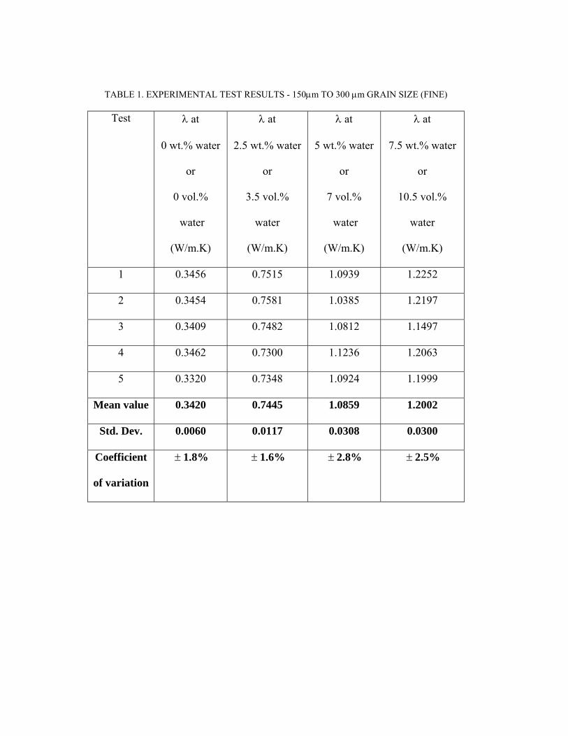
TABLE 1. EXPERIMENTAL TEST RESULTS - 150µm TO 300 µm GRAIN SIZE (FINE)
Test λ at
0 wt.% water
or
0 vol.%
water
(W/m.K)
λ at
2.5 wt.% water
or
3.5 vol.%
water
(W/m.K)
λ at
5 wt.% water
or
7 vol.%
water
(W/m.K)
λ at
7.5 wt.% water
or
10.5 vol.%
water
(W/m.K)
1 0.3456 0.7515 1.0939 1.2252
2 0.3454 0.7581 1.0385 1.2197
3 0.3409 0.7482 1.0812 1.1497
4 0.3462 0.7300 1.1236 1.2063
5 0.3320 0.7348 1.0924 1.1999
Mean value 0.3420 0.7445 1.0859 1.2002
Std. Dev. 0.0060 0.0117 0.0308 0.0300
Coefficient
of variation
± 1.8% ± 1.6% ± 2.8% ± 2.5%
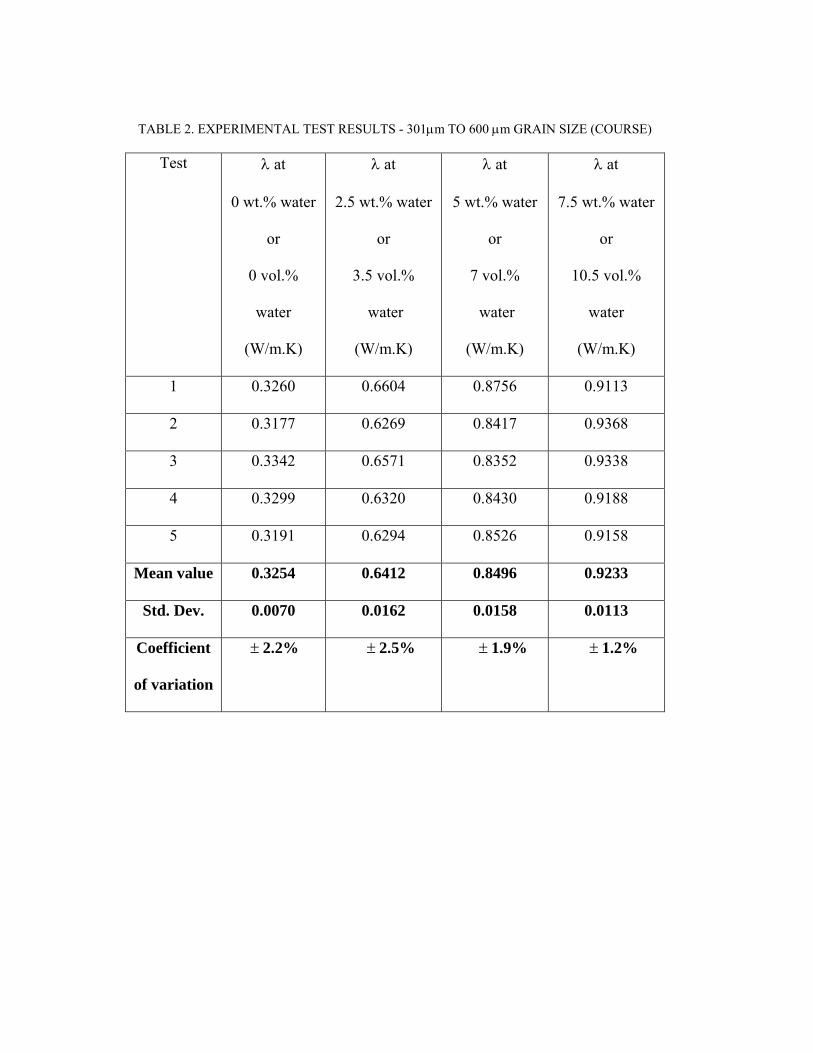
TABLE 2. EXPERIMENTAL TEST RESULTS - 301µm TO 600 µm GRAIN SIZE (COURSE)
Test λ at
0 wt.% water
or
0 vol.%
water
(W/m.K)
λ at
2.5 wt.% water
or
3.5 vol.%
water
(W/m.K)
λ at
5 wt.% water
or
7 vol.%
water
(W/m.K)
λ at
7.5 wt.% water
or
10.5 vol.%
water
(W/m.K)
1 0.3260 0.6604 0.8756 0.9113
2 0.3177 0.6269 0.8417 0.9368
3 0.3342 0.6571 0.8352 0.9338
4 0.3299 0.6320 0.8430 0.9188
5 0.3191 0.6294 0.8526 0.9158
Mean value 0.3254 0.6412 0.8496 0.9233
Std. Dev. 0.0070 0.0162 0.0158 0.0113
Coefficient
of variation
± 2.2% ± 2.5% ± 1.9% 1.2% ±
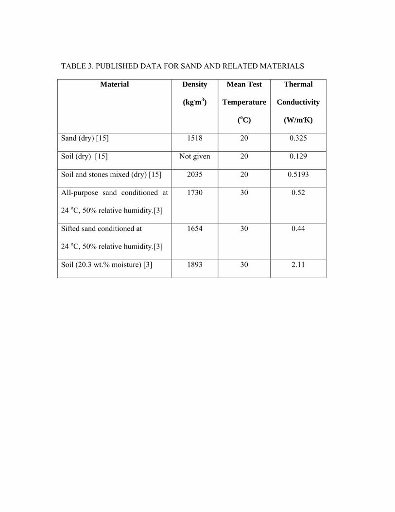
TABLE 3. PUBLISHED DATA FOR SAND AND RELATED MATERIALS
Material Density
(kg.m3)
Mean Test
Temperature
(oC)
Thermal
Conductivity
(W/m.K)
Sand (dry) [15] 1518 20 0.325
Soil (dry) [15] Not given 20 0.129
Soil and stones mixed (dry) [15] 2035 20 0.5193
All-purpose sand conditioned at
24 oC, 50% relative humidity.[3]
1730 30 0.52
Sifted sand conditioned at
24 oC, 50% relative humidity.[3]
1654 30 0.44
Soil (20.3 wt.% moisture) [3] 1893 30 2.11
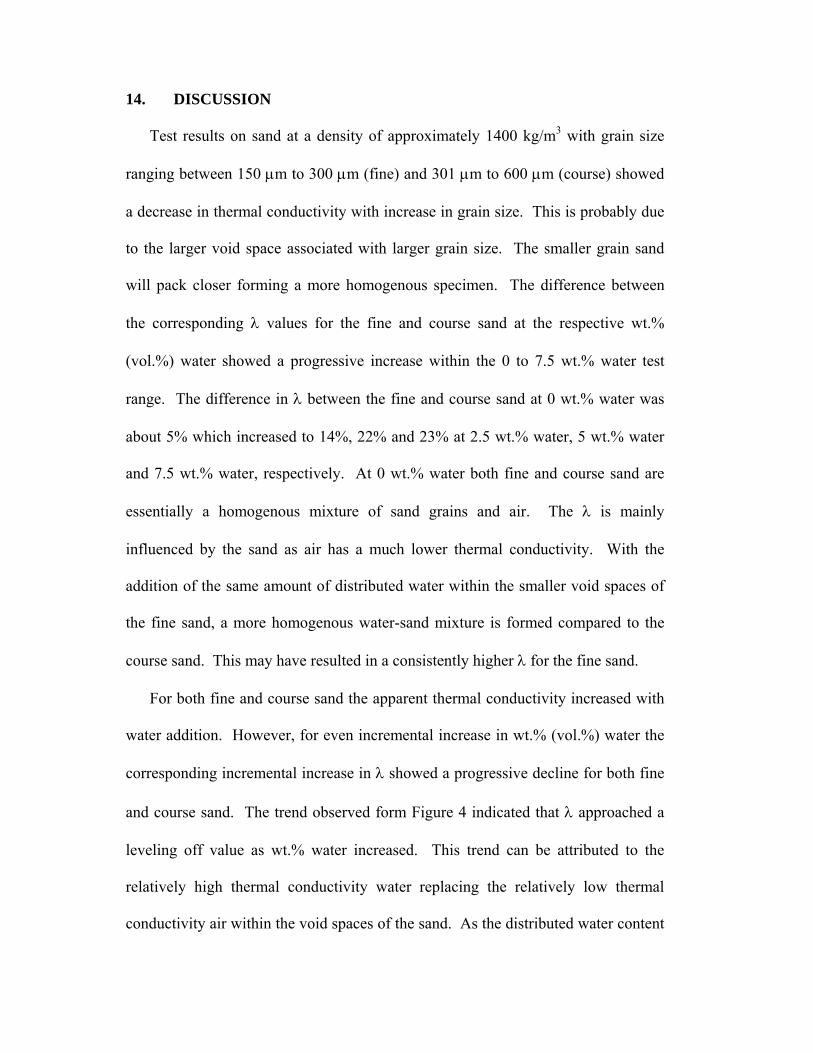
14. DISCUSSION
Test results on sand at a density of approximately 1400 kg/m3 with grain size
ranging between 150 µm to 300 µm (fine) and 301 µm to 600 µm (course) showed
a decrease in thermal conductivity with increase in grain size. This is probably due
to the larger void space associated with larger grain size. The smaller grain sand
will pack closer forming a more homogenous specimen. The difference between
the corresponding λ values for the fine and course sand at the respective wt.%
(vol.%) water showed a progressive increase within the 0 to 7.5 wt.% water test
range. The difference in λ between the fine and course sand at 0 wt.% water was
about 5% which increased to 14%, 22% and 23% at 2.5 wt.% water, 5 wt.% water
and 7.5 wt.% water, respectively. At 0 wt.% water both fine and course sand are
essentially a homogenous mixture of sand grains and air. The λ is mainly
influenced by the sand as air has a much lower thermal conductivity. With the
addition of the same amount of distributed water within the smaller void spaces of
the fine sand, a more homogenous water-sand mixture is formed compared to the
course sand. This may have resulted in a consistently higher λ for the fine sand.
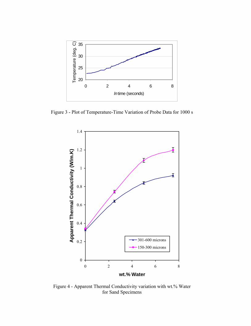
For both fine and course sand the apparent thermal conductivity increased with
water addition. However, for even incremental increase in wt.% (vol.%) water the
corresponding incremental increase in λ showed a progressive decline for both fine
and course sand. The trend observed form Figure 4 indicated that λ approached a
leveling off value as wt.% water increased. This trend can be attributed to the
relatively high thermal conductivity water replacing the relatively low thermal
conductivity air within the void spaces of the sand. As the distributed water content

increased and the void spaces filled with water the material became a homogenous
mixture of water and sand. This trend and the λ range reported are consistent with
published data [4,5,14] and the experimentally determined λ was within the range
of published dada listed in Table 3.
15. CONCLUSIONS
• The apparent thermal conductivity (λ) of sand with grain size 150µm to
300µm (fine) is higher than sand with grain size 301µm to 600µm (course).
• For 7.5 wt.% water the fine sand showed a 30% higher λ than the course
sand.
• For even incremental increase in water content the corresponding
incremental increase in λ gets smaller within the 0 to 7.5 wt.% range.
• Above 7.5 wt.% water the λ value tends to levels off.
16. WORK IN PROGRESS
Testing on another grain size range is being conducted to look at the variation of
λ with grain size at the respective percentage moisture content of '‘sharp sand’ and
to develop a correlation for λ with grain size and moisture.
17. REFERENCES
1. Swanson, R. G.(1970). Sample Examination Manual. Methods in Exploration
Series, The American Association of Petroleum Geologists, Tulsa, Oklahoma,
USA, pp. IV-15 – IV-26.
2. Carslaw, H. S. and J. C. Jaeger. (1964). Conduction of Heat in Solids. Oxford
Press, 2nd ed., pp. 58-60, 344-345.
3. Manohar, K., D. W. Yarbrough, and J. R. Booth. (2000). “Measurement of
Apparent Thermal Conductivity by the Thermal Probe Method,” Journal of
Testing and Evaluation, JTEVA, 28(5):345-351.
4. Ghuman, B. S., and R. Lal. (1985). “Thermal Conductivity, Thermal
Diffusivity, and Thermal Capacity of Some Nigerian Siols,” Soil Science,
139(1):74-80.
5. Abu-Hamdah, N. H. (2000). “Effect of Tillage Treatments on Soil Thermal
Conductivity of Sone Jordanian Clay Loam and Loam Siol,” Soil Tillage
Research, 56:145-151.
6. American Society for Testing and Materials.(1995). “Standard Test Method for
Determination of Thermal Conductivity of Soil and Soft Rock by Thermal
Needle Probe Procedure,” Annual Book of ASTM Standards, ASTM D
5334:225-229.
7. Winterkorn, H. F.(1970). “Suggested Method of Test for Thermal Resistivity of
Soil by the Thermal Probe,” Special Procedure for testing Soil and Rock for
Engineering Purposes, ASTM STP 479:264-270.
8. Coleman, H. W., and W. G. Steller. (1999). “Experimentation and Uncertainty
Analysis for Engineers,” 2nd ed., John Wiley and Sons, New York, pp. 47-64.
9. EXTECH Instruments. (2002). “Mocro-Controler Based DC Power Supply,”
Instruction Manual, Bear Hill Road, Walthan, MA, USA.
10. Weast, R. C. (1982). CRC Handbook of Chemistry and Physics. CRC Press
Inc., 62nd ed., p. E-82.
11. Kersten, M. S.(1949). “Thermal Properties of Soils,” Bulletin of the University
of Minnesota Institute of Technology, Engineering Experiment Station, LII(28).
12. Natrella, M. G.(1963). “Experimental Statistics,” National Bureau of Standards
Handbook, No. 91,
13. LaserComp FOX 304, “Heat Flow Meter Thermal Conductivity Instrument,”
Information Sheet, LaserComp, Wakefield, MA, USA.
14. Douglas, E. and E. McKyes. (1978). “Compaction Effects on the Hydraulic
Conductivity of a Clay Soil,” Soil Science, 125(5):278-282.
15. Avallone, E. A. and Baumeister, T. (1996). Marks’ Standard Handbook for
Mechanical Engineers, 10th ed., McGraw-Hill, New York, p. 4-83.
Thermal Conductivity of Trinidad ‘Guanapo Sharp Sand’
Krishpersad Manohar, Lecturer, Mechanical and Manufacturing Engineering Department, The University of the West Indies, St. Augustine, Trinidad, West
Indies. Email: [email protected] Kimberly Ramroop, M.Phil. Candidate, Mechanical and Manufacturing
Engineering Department, The University of the West Indies, St. Augustine, Trinidad, West Indies.
Gurmohan S. Kochhar, Professor, Department of Mechanical & Manufacturing Engineering, The University of the West Indies, St. Augustine, Trinidad, West
Indies. Email: [email protected]
List of Figure Titles
Figure 1 - Schematic of thermal probe Figure 2 - Schematic of electrical circuit and data acquisition system Figure 3 - Plot of Temperature-Time Variation of Probe Data for 1000 s Figure 4 - Apparent Thermal Conductivity variation with wt.% Water for Sand Specimens
Thermocouple wire
Figure 2
Nylon cap
Steel probe
Thermocouple-
Epox
Heater wire
Figure 1 - Schematic o
Schematic of electrical circuit
50 mm
50 mm
f the
and
10 mm
rmal probe
data acquisition system
20
25
30
35
0 2 4 6
ln time (seconds)
Tem
pera
ture
(deg
. C)
8
Figure 3 - Plot of Temperature-Time Variation of Probe Data for 1000 s
0
0.2
0.4
0.6
0.8
1
1.2
1.4
0 2 4 6 8
wt.% Water
App
aren
t The
rmal
Con
duct
ivity
(W/m
.K)
301-600 microns
150-300 microns
Figure 4 - Apparent Thermal Conductivity variation with wt.% Water
for Sand Specimens
Recommended