arX
iv:1
405.
4980
v1 [
mat
h.O
C]
20
May
201
4 Theory of Convex Optimization for MachineLearning
Sebastien Bubeck1
1 Department of Operations Research and Financial Engineering, PrincetonUniversity, Princeton 08544, USA, [email protected]
Abstract
This monograph presents the main mathematical ideas in convex opti-
mization. Starting from the fundamental theory of black-box optimiza-
tion, the material progresses towards recent advances in structural op-
timization and stochastic optimization. Our presentation of black-box
optimization, strongly influenced by the seminal book of Nesterov, in-
cludes the analysis of the Ellipsoid Method, as well as (accelerated) gra-
dient descent schemes. We also pay special attention to non-Euclidean
settings (relevant algorithms include Frank-Wolfe, Mirror Descent, and
Dual Averaging) and discuss their relevance in machine learning. We
provide a gentle introduction to structural optimization with FISTA (to
optimize a sum of a smooth and a simple non-smooth term), Saddle-
Point Mirror Prox (Nemirovski’s alternative to Nesterov’s smoothing),
and a concise description of Interior Point Methods. In stochastic op-
timization we discuss Stochastic Gradient Descent, mini-batches, Ran-
dom Coordinate Descent, and sublinear algorithms. We also briefly
touch upon convex relaxation of combinatorial problems and the use of
randomness to round solutions, as well as random walks based methods.

Contents
1 Introduction 1
1.1 Some convex optimization problems for machine learning 2
1.2 Basic properties of convexity 3
1.3 Why convexity? 6
1.4 Black-box model 7
1.5 Structured optimization 8
1.6 Overview of the results 9
2 Convex optimization in finite dimension 12
2.1 The center of gravity method 12
2.2 The ellipsoid method 14
3 Dimension-free convex optimization 19
3.1 Projected Subgradient Descent for Lipschitz functions 20
3.2 Gradient descent for smooth functions 23
3.3 Conditional Gradient Descent, aka Frank-Wolfe 28
3.4 Strong convexity 33
i

ii Contents
3.5 Lower bounds 37
3.6 Nesterov’s Accelerated Gradient Descent 41
4 Almost dimension-free convex optimization in
non-Euclidean spaces 48
4.1 Mirror maps 50
4.2 Mirror Descent 51
4.3 Standard setups for Mirror Descent 53
4.4 Lazy Mirror Descent, aka Nesterov’s Dual Averaging 55
4.5 Mirror Prox 57
4.6 The vector field point of view on MD, DA, and MP 59
5 Beyond the black-box model 61
5.1 Sum of a smooth and a simple non-smooth term 62
5.2 Smooth saddle-point representation of a non-smooth
function 64
5.3 Interior Point Methods 70
6 Convex optimization and randomness 81
6.1 Non-smooth stochastic optimization 82
6.2 Smooth stochastic optimization and mini-batch SGD 84
6.3 Improved SGD for a sum of smooth and strongly convex
functions 86
6.4 Random Coordinate Descent 90
6.5 Acceleration by randomization for saddle points 94
6.6 Convex relaxation and randomized rounding 96
6.7 Random walk based methods 100

1
Introduction
The central objects of our study are convex functions and convex sets
in Rn.
Definition 1.1 (Convex sets and convex functions). A set X ⊂Rn is said to be convex if it contains all of its segments, that is
∀(x, y, γ) ∈ X × X × [0, 1], (1− γ)x+ γy ∈ X .
A function f : X → R is said to be convex if it always lies below its
chords, that is
∀(x, y, γ) ∈ X × X × [0, 1], f((1− γ)x+ γy) ≤ (1− γ)f(x) + γf(y).
We are interested in algorithms that take as input a convex set X and
a convex function f and output an approximate minimum of f over X .
We write compactly the problem of finding the minimum of f over Xas
min. f(x)
s.t. x ∈ X .
1

2 Introduction
In the following we will make more precise how the set of constraints Xand the objective function f are specified to the algorithm. Before that
we proceed to give a few important examples of convex optimization
problems in machine learning.
1.1 Some convex optimization problems for machine learning
Many fundamental convex optimization problems for machine learning
take the following form:
minx∈Rn
m∑
i=1
fi(x) + λR(x), (1.1)
where the functions f1, . . . , fm,R are convex and λ ≥ 0 is a fixed
parameter. The interpretation is that fi(x) represents the cost of
using x on the ith element of some data set, and R(x) is a regular-
ization term which enforces some ”simplicity” in x. We discuss now
major instances of (1.1). In all cases one has a data set of the form
(wi, yi) ∈ Rn×Y, i = 1, . . . ,m and the cost function fi depends only on
the pair (wi, yi). We refer to Hastie et al. [2001], Scholkopf and Smola
[2002] for more details on the origin of these important problems.
In classification one has Y = −1, 1. Taking fi(x) =
max(0, 1 − yix⊤wi) (the so-called hinge loss) and R(x) = ‖x‖22
one obtains the SVM problem. On the other hand taking
fi(x) = log(1+exp(−yix⊤wi)) (the logistic loss) and againR(x) = ‖x‖22one obtains the logistic regression problem.
In regression one has Y = R. Taking fi(x) = (x⊤wi − yi)2 and
R(x) = 0 one obtains the vanilla least-squares problem which can be
rewritten in vector notation as
minx∈Rn
‖Wx− Y ‖22,
where W ∈ Rm×n is the matrix with w⊤
i on the ith row and
Y = (y1, . . . , yn)⊤. With R(x) = ‖x‖22 one obtains the ridge regression
problem, while with R(x) = ‖x‖1 this is the LASSO problem.

1.2. Basic properties of convexity 3
In our last example the design variable x is best viewed as a matrix,
and thus we denote it by a capital letter X. Here our data set consists
of observations of some of the entries of an unknown matrix Y , and we
want to ”complete” the unobserved entries of Y in such a way that the
resulting matrix is ”simple” (in the sense that it has low rank). After
some massaging (see Candes and Recht [2009]) the matrix completion
problem can be formulated as follows:
min. Tr(X)
s.t. X ∈ Rn×n,X⊤ = X,X 0,Xi,j = Yi,j for (i, j) ∈ Ω,
where Ω ⊂ [n]2 and (Yi,j)(i,j)∈Ω are given.
1.2 Basic properties of convexity
A basic result about convex sets that we shall use extensively is the
Separation Theorem.
Theorem 1.1 (Separation Theorem). Let X ⊂ Rn be a closed
convex set, and x0 ∈ Rn \ X . Then, there exists w ∈ R
n and t ∈ R
such that
w⊤x0 < t, and ∀x ∈ X , w⊤x ≥ t.
Note that if X is not closed then one can only guarantee that
w⊤x0 ≤ w⊤x,∀x ∈ X (and w 6= 0). This immediately implies the
Supporting Hyperplane Theorem:
Theorem 1.2 (Supporting Hyperplane Theorem). Let X ⊂ Rn
be a convex set, and x0 ∈ ∂X . Then, there exists w ∈ Rn, w 6= 0 such
that
∀x ∈ X , w⊤x ≥ w⊤x0.
We introduce now the key notion of subgradients.

4 Introduction
Definition 1.2 (Subgradients). Let X ⊂ Rn, and f : X → R. Then
g ∈ Rn is a subgradient of f at x ∈ X if for any y ∈ X one has
f(x)− f(y) ≤ g⊤(x− y).
The set of subgradients of f at x is denoted ∂f(x).
The next result shows (essentially) that a convex functions always
admit subgradients.
Proposition 1.1 (Existence of subgradients). Let X ⊂ Rn be
convex, and f : X → R. If ∀x ∈ X , ∂f(x) 6= ∅ then f is convex. Con-
versely if f is convex then for any x ∈ int(X ), ∂f(x) 6= ∅. Furthermore
if f is convex and differentiable at x then ∇f(x) ∈ ∂f(x).
Before going to the proof we recall the definition of the epigraph of
a function f : X → R:
epi(f) = (x, t) ∈ X × R : t ≥ f(x).
It is obvious that a function is convex if and only if its epigraph is a
convex set.
Proof. The first claim is almost trivial: let g ∈ ∂f((1− γ)x+ γy), then
by definition one has
f((1− γ)x+ γy) ≤ f(x) + γg⊤(y − x),
f((1− γ)x+ γy) ≤ f(y) + (1− γ)g⊤(x− y),
which clearly shows that f is convex by adding the two (appropriately
rescaled) inequalities.
Now let us prove that a convex function f has subgradients in the
interior of X . We build a subgradient by using a supporting hyperplane
to the epigraph of the function. Let x ∈ X . Then clearly (x, f(x)) ∈∂epi(f), and epi(f) is a convex set. Thus by using the Supporting
Hyperplane Theorem, there exists (a, b) ∈ Rn × R such that
a⊤x+ bf(x) ≥ a⊤y + bt,∀(y, t) ∈ epi(f). (1.2)

1.2. Basic properties of convexity 5
Clearly, by letting t tend to infinity, one can see that b ≤ 0. Now let
us assume that x is in the interior of X . Then for ε > 0 small enough,
y = x+εa ∈ X , which implies that b cannot be equal to 0 (recall that if
b = 0 then necessarily a 6= 0 which allows to conclude by contradiction).
Thus rewriting (1.2) for t = f(y) one obtains
f(x)− f(y) ≤ 1
|b|a⊤(x− y).
Thus a/|b| ∈ ∂f(x) which concludes the proof of the second claim.
Finally let f be a convex and differentiable function. Then by defi-
nition:
f(y) ≥ f((1− γ)x+ γy)− (1− γ)f(x)
γ
= f(x) +f(x+ γ(y − x))− f(x)
γ
→γ→0
f(x) +∇f(x)⊤(y − x),
which shows that ∇f(x) ∈ ∂f(x).
In several cases of interest the set of contraints can have an empty
interior, in which case the above proposition does not yield any informa-
tion. However it is easy to replace int(X ) by ri(X ) -the relative interior
of X - which is defined as the interior of X when we view it as subset of
the affine subspace it generates. Other notions of convex analysis will
prove to be useful in some parts of this text. In particular the notion
of closed convex functions is convenient to exclude pathological cases:
these are the convex functions with closed epigraphs. Sometimes it is
also useful to consider the extension of a convex function f : X → R to
a function from Rn to R by setting f(x) = +∞ for x 6∈ X . In convex
analysis one uses the term proper convex function to denote a convex
function with values in R ∪ +∞ such that there exists x ∈ Rn with
f(x) < +∞. From now on all convex functions will be closed,
and if necessary we consider also their proper extension. We
refer the reader to Rockafellar [1970] for an extensive discussion of these
notions.

6 Introduction
1.3 Why convexity?
The key to the algorithmic success in minimizing convex functions is
that these functions exhibit a local to global phenomenon. We have
already seen one instance of this in Proposition 1.1, where we showed
that ∇f(x) ∈ ∂f(x): the gradient ∇f(x) contains a priori only local
information about the function f around x while the subdifferential
∂f(x) gives a global information in the form of a linear lower bound on
the entire function. Another instance of this local to global phenomenon
is that local minima of convex functions are in fact global minima:
Proposition 1.2 (Local minima are global minima). Let f be
convex. If x is a local minimum of f then x is a global minimum of f .
Furthermore this happens if and only if 0 ∈ ∂f(x).
Proof. Clearly 0 ∈ ∂f(x) if and only if x is a global minimum of f .
Now assume that x is local minimum of f . Then for γ small enough
one has for any y,
f(x) ≤ f((1− γ)x+ γy) ≤ (1− γ)f(x) + γf(y),
which implies f(x) ≤ f(y) and thus x is a global minimum of f .
The nice behavior of convex functions will allow for very fast algo-
rithms to optimize them. This alone would not be sufficient to justify
the importance of this class of functions (after all constant functions
are pretty easy to optimize). However it turns out that surprisingly
many optimization problems admit a convex (re)formulation. The ex-
cellent book Boyd and Vandenberghe [2004] describes in great details
the various methods that one can employ to uncover the convex aspects
of an optimization problem. We will not repeat these arguments here,
but we have already seen that many famous machine learning prob-
lems (SVM, ridge regression, logistic regression, LASSO, and matrix
completion) are immediately formulated as convex problems.
We conclude this section with a simple extension of the optimality
condition ”0 ∈ ∂f(x)” to the case of constrained optimization. We state
this result in the case of a differentiable function for sake of simplicity.

1.4. Black-box model 7
Proposition 1.3 (First order optimality condition). Let f be
convex and X a closed convex set on which f is differentiable. Then
x∗ ∈ argminx∈X
f(x),
if and only if one has
∇f(x∗)⊤(x∗ − y) ≤ 0,∀y ∈ X .
Proof. The ”if” direction is trivial by using that a gradient is also
a subgradient. For the ”only if” direction it suffices to note that if
∇f(x)⊤(y − x) < 0, then f is locally decreasing around x on the line
to y (simply consider h(t) = f(x + t(y − x)) and note that h′(0) =
∇f(x)⊤(y − x)).
1.4 Black-box model
We now describe our first model of ”input” for the objective function
and the set of constraints. In the black-box model we assume that
we have unlimited computational resources, the set of constraint X is
known, and the objective function f : X → R is unknown but can be
accessed through queries to oracles:
• A zeroth order oracle takes as input a point x ∈ X and
outputs the value of f at x.• A first order oracle takes as input a point x ∈ X and outputs
a subgradient of f at x.
In this context we are interested in understanding the oracle complexity
of convex optimization, that is how many queries to the oracles are
necessary and sufficient to find an ε-approximate minima of a convex
function. To show an upper bound on the sample complexity we
need to propose an algorithm, while lower bounds are obtained by
information theoretic reasoning (we need to argue that if the number
of queries is ”too small” then we don’t have enough information about
the function to identify an ε-approximate solution).

8 Introduction
From a mathematical point of view, the strength of the black-box
model is that it will allow us to derive a complete theory of convex
optimization, in the sense that we will obtain matching upper and
lower bounds on the oracle complexity for various subclasses of inter-
esting convex functions. While the model by itself does not limit our
computational resources (for instance any operation on the constraint
set X is allowed) we will of course pay special attention to the
computational complexity (i.e., the number of elementary operations
that the algorithm needs to do) of our proposed algorithms.
The black-box model was essentially developped in the early days
of convex optimization (in the Seventies) with Nemirovski and Yudin
[1983] being still an important reference for this theory. In the recent
years this model and the corresponding algorithms have regained a lot
of popularity, essentially for two reasons:
• It is possible to develop algorithms with dimension-free or-
acle complexity which is quite attractive for optimization
problems in very high dimension.• Many algorithms developped in this model are robust to noise
in the output of the oracles. This is especially interesting for
stochastic optimization, and very relevant to machine learn-
ing applications. We will explore this in details in Chapter
6.
Chapter 2, Chapter 3 and Chapter 4 are dedicated to the study of
the black-box model (noisy oracles are discussed in Chapter 6). We do
not cover the setting where only a zeroth order oracle is available, also
called derivative free optimization, and we refer to Conn et al. [2009],
Audibert et al. [2011] for further references on this.
1.5 Structured optimization
The black-box model described in the previous section seems extremely
wasteful for the applications we discussed in Section 1.1. Consider for
instance the LASSO objective: x 7→ ‖Wx− y‖22 + ‖x‖1. We know this
function globally, and assuming that we can only make local queries

1.6. Overview of the results 9
through oracles seem like an artificial constraint for the design of
algorithms. Structured optimization tries to address this observation.
Ultimately one would like to take into account the global structure
of both f and X in order to propose the most efficient optimization
procedure. An extremely powerful hammer for this task are the
Interior Point Methods. We will describe this technique in Chapter 5
alongside with other more recent techniques such as FISTA or Mirror
Prox.
We briefly describe now two classes of optimization problems for
which we will be able to exploit the structure very efficiently, these
are the LPs (Linear Programs) and SDPs (Semi-Definite Programs).
Ben-Tal and Nemirovski [2001] describe a more general class of Conic
Programs but we will not go in that direction here.
The class LP consists of problems where f(x) = c⊤x for some c ∈Rn, and X = x ∈ R
n : Ax ≤ b for some A ∈ Rm×n and b ∈ R
m.
The class SDP consists of problems where the optimization vari-
able is a symmetric matrix X ∈ Rn×n. Let S
n be the space of n × n
symmetric matrices (respectively Sn+ is the space of positive semi-
definite matrices), and let 〈·, ·〉 be the Frobenius inner product (re-
call that it can be written as 〈A,B〉 = Tr(A⊤B)). In the class SDP
the problems are of the following form: f(x) = 〈X,C〉 for some
C ∈ Rn×n, and X = X ∈ S
n+ : 〈X,Ai〉 ≤ bi, i ∈ 1, . . . ,m for
some A1, . . . , Am ∈ Rn×n and b ∈ R
m. Note that the matrix comple-
tion problem described in Section 1.1 is an example of an SDP.
1.6 Overview of the results
Table 1.1 can be used as a quick reference to the results proved in
Chapter 2 to Chapter 5. The results of Chapter 6 are the most relevant
to machine learning, but they are also slightly more specific which
makes them harder to summarize.
In the entire monograph the emphasis is on presenting the algo-
rithms and proofs in the simplest way. This comes at the expense
of making the algorithms more practical. For example we always

10 Introduction
assume a fixed number of iterations t, and the algorithms we consider
can depend on t. Similarly we assume that the relevant parameters
describing the regularity of the objective function (Lipschitz constant,
smoothness constant, strong convexity parameter) are know and can
also be used to tune the algorithm’s own parameters. The interested
reader can find guidelines to adapt to these potentially unknown
parameters in the references given in the text.
Notation. We always denote by x∗ a point in X such that f(x∗) =minx∈X f(x) (note that the optimization problem under consideration
will always be clear from the context). In particular we always assume
that x∗ exists. For a vector x ∈ Rn we denote by x(i) its ith coordinate.
The dual of a norm ‖ · ‖ (defined later) will be denoted either ‖ · ‖∗ or
‖·‖∗ (depending on whether the norm already comes with a subscript).
Other notation are standard (e.g., In for the n × n identity matrix, for the positive semi-definite order on matrices, etc).

1.6. Overview of the results 11
f Algorithm Rate # Iterations Cost per iteration
non-smoothCenter of
Gravityexp(−t/n) n log(1/ε)
one gradient,
one n-dim integral
non-smoothEllipsoid
MethodRr exp(−t/n2) n2 log(R/(rε))
one gradient,
separation oracle,
matrix-vector mult.
non-smooth,
LipschitzPGD RL/
√t R2L2/ε2
one gradient,
one projection
smooth PGD βR2/t βR2/εone gradient,
one projection
smoothNesterov’s
AGDβR2/t2 R
√β/ε one gradient
smooth
(arbitrary norm)FW βR2/t βR2/ε
one gradient,
one linear opt.
strongly convex,
LipschitzPGD L2/(αt) L2/(αε)
one gradient,
one projection
strongly convex,
smoothPGD R2 exp(−t/Q) Q log(R2/ε)
one gradient,
one projection
strongly convex,
smooth
Nesterov’s
AGDR2 exp(−t/√Q)
√Q log(R2/ε) one gradient
f + g,
f smooth,
g simple
FISTA βR2/t2 R√β/ε
one gradient of f
Prox. step with g
maxy∈Y ϕ(x, y),ϕ smooth
SP-MP βR2/t βR2/εMD step on XMD step on Y
c⊤x,X with F
ν-self-conc.
IPM νO(1) exp(−t/√ν) √ν log(ν/ε)
Newton direction
for F on XTable 1.1 Summary of the results proved in this monograph.
2
Convex optimization in finite dimension
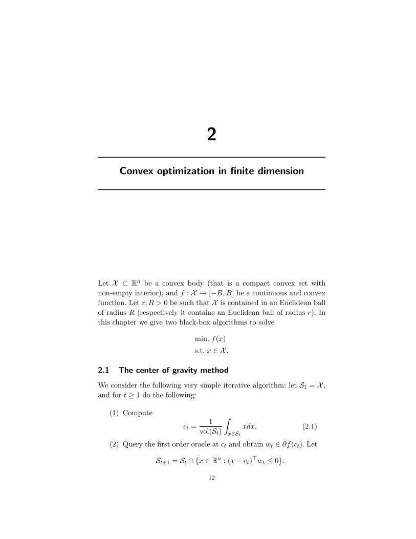
Let X ⊂ Rn be a convex body (that is a compact convex set with
non-empty interior), and f : X → [−B,B] be a continuous and convex
function. Let r,R > 0 be such that X is contained in an Euclidean ball
of radius R (respectively it contains an Euclidean ball of radius r). In
this chapter we give two black-box algorithms to solve
min. f(x)
s.t. x ∈ X .
2.1 The center of gravity method
We consider the following very simple iterative algorithm: let S1 = X ,
and for t ≥ 1 do the following:
(1) Compute
ct =1
vol(St)
∫
x∈St
xdx. (2.1)
(2) Query the first order oracle at ct and obtain wt ∈ ∂f(ct). Let
St+1 = St ∩ x ∈ Rn : (x− ct)
⊤wt ≤ 0.
12

2.1. The center of gravity method 13
If stopped after t queries to the first order oracle then we use t queries
to a zeroth order oracle to output
xt ∈ argmin1≤r≤t
f(cr).
This procedure is known as the center of gravity method, it was dis-
covered independently on both sides of the Wall by Levin [1965] and
Newman [1965].
Theorem 2.1. The center of gravity method satisfies
f(xt)−minx∈X
f(x) ≤ 2B
(1− 1
e
)t/n
.
Before proving this result a few comments are in order.
To attain an ε-optimal point the center of gravity method requires
O(n log(2B/ε)) queries to both the first and zeroth order oracles. It can
be shown that this is the best one can hope for, in the sense that for
ε small enough one needs Ω(n log(1/ε)) calls to the oracle in order to
find an ε-optimal point, see Nemirovski and Yudin [1983] for a formal
proof.
The rate of convergence given by Theorem 2.1 is exponentially fast.
In the optimization literature this is called a linear rate for the following
reason: the number of iterations required to attain an ε-optimal point
is proportional to log(1/ε), which means that to double the number of
digits in accuracy one needs to double the number of iterations, hence
the linear nature of the convergence rate.
The last and most important comment concerns the computational
complexity of the method. It turns out that finding the center of gravity
ct is a very difficult problem by itself, and we do not have computation-
ally efficient procedure to carry this computation in general. In Section
6.7 we will discuss a relatively recent (compared to the 50 years old
center of gravity method!) breakthrough that gives a randomized algo-
rithm to approximately compute the center of gravity. This will in turn
give a randomized center of gravity method which we will describe in
details.
We now turn to the proof of Theorem 2.1. We will use the following
elementary result from convex geometry:

14 Convex optimization in finite dimension
Lemma 2.1 (Grunbaum [1960]). Let K be a centered convex set,
i.e.,∫x∈K xdx = 0, then for any w ∈ R
n, w 6= 0, one has
Vol(K ∩ x ∈ R
n : x⊤w ≥ 0)≥ 1
eVol(K).
We now prove Theorem 2.1.
Proof. Let x∗ be such that f(x∗) = minx∈X f(x). Since wt ∈ ∂f(ct)
one has
f(ct)− f(x) ≤ w⊤t (ct − x).
and thus
St \St+1 ⊂ x ∈ X : (x− ct)⊤wt > 0 ⊂ x ∈ X : f(x) > f(ct), (2.2)
which clearly implies that one can never remove the optimal point
from our sets in consideration, that is x∗ ∈ St for any t. Without loss
of generality we can assume that we always have wt 6= 0, for otherwise
one would have f(ct) = f(x∗) which immediately conludes the proof.
Now using that wt 6= 0 for any t and Lemma 2.1 one clearly obtains
vol(St+1) ≤(1− 1
e
)t
vol(X ).
For ε ∈ [0, 1], let Xε = (1 − ε)x∗ + εx, x ∈ X. Note that vol(Xε) =
εnvol(X ). These volume computations show that for ε >(1− 1
e
)t/n
one has vol(Xε) > vol(St+1). In particular this implies that for ε >(1− 1
e
)t/n, there must exist a time r ∈ 1, . . . , t, and xε ∈ Xε, such
that xε ∈ Sr and xε 6∈ Sr+1. In particular by (2.2) one has f(cr) <
f(xε). On the other hand by convexity of f one clearly has f(xε) ≤f(x∗) + 2εB. This concludes the proof.
2.2 The ellipsoid method
Recall that an ellipsoid is a convex set of the form
E = x ∈ Rn : (x− c)⊤H−1(x− c) ≤ 1,

2.2. The ellipsoid method 15
where c ∈ Rn, and H is a symmetric positive definite matrix. Geomet-
rically c is the center of the ellipsoid, and the semi-axes of E are given
by the eigenvectors of H, with lengths given by the square root of the
corresponding eigenvalues.
We give now a simple geometric lemma, which is at the heart of the
ellipsoid method.
Lemma 2.2. Let E0 = x ∈ Rn : (x− c0)
⊤H−10 (x− c0) ≤ 1. For any
w ∈ Rn, w 6= 0, there exists an ellipsoid E such that
E ⊃ x ∈ E0 : w⊤(x− c0) ≤ 0, (2.3)
and
vol(E) ≤ exp
(− 1
2n
)vol(E0). (2.4)
Furthermore for n ≥ 2 one can take E = x ∈ Rn : (x−c)⊤H−1(x−c) ≤
1 where
c = c0 −1
n+ 1
H0w√w⊤H0w
, (2.5)
H =n2
n2 − 1
(H0 −
2
n+ 1
H0ww⊤H0
w⊤H0w
). (2.6)
Proof. For n = 1 the result is obvious, in fact we even have vol(E) ≤12vol(E0).
For n ≥ 2 one can simply verify that the ellipsoid given by (2.5)
and (2.6) satisfy the required properties (2.3) and (2.4). Rather than
bluntly doing these computations we will show how to derive (2.5) and
(2.6). As a by-product this will also show that the ellipsoid defined by
(2.5) and (2.6) is the unique ellipsoid of minimal volume that satisfy
(2.3). Let us first focus on the case where E0 is the Euclidean ball
B = x ∈ Rn : x⊤x ≤ 1. We momentarily assume that w is a unit
norm vector.
By doing a quick picture, one can see that it makes sense to look
for an ellipsoid E that would be centered at c = −tw, with t ∈ [0, 1]
(presumably t will be small), and such that one principal direction

16 Convex optimization in finite dimension
is w (with inverse squared semi-axis a > 0), and the other principal
directions are all orthogonal to w (with the same inverse squared semi-
axes b > 0). In other words we are looking for E = x : (x−c)⊤H−1(x−c) ≤ 1 with
c = −tw, and H−1 = aww⊤ + b(In − ww⊤).
Now we have to express our constraints on the fact that E should
contain the half Euclidean ball x ∈ B : x⊤w ≤ 0. Since we are also
looking for E to be as small as possible, it makes sense to ask for Eto ”touch” the Euclidean ball, both at x = −w, and at the equator
∂B ∩ w⊥. The former condition can be written as:
(−w − c)⊤H−1(−w − c) = 1 ⇔ (t− 1)2a = 1,
while the latter is expressed as:
∀y ∈ ∂B ∩ w⊥, (y − c)⊤H−1(y − c) = 1 ⇔ b+ t2a = 1.
As one can see from the above two equations, we are still free to choose
any value for t ∈ [0, 1/2) (the fact that we need t < 1/2 comes from
b = 1−(
tt−1
)2> 0). Quite naturally we take the value that minimizes
the volume of the resulting ellipsoid. Note that
vol(E)vol(B) =
1√a
(1√b
)n−1
=1√
1(1−t)2
(1−
(t
1−t
)2)n−1=
1√f(
11−t
) ,
where f(h) = h2(2h−h2)n−1. Elementary computations show that the
maximum of f (on [1, 2]) is attained at h = 1 + 1n (which corresponds
to t = 1n+1), and the value is
(1 +
1
n
)2(1− 1
n2
)n−1
≥ exp
(1
n
),
where the lower bound follows again from elementary computations.
Thus we showed that, for E0 = B, (2.3) and (2.4) are satisfied with the
following ellipsoid:x :
(x+
w/‖w‖2n+ 1
)⊤(n2 − 1
n2In +
2(n + 1)
n2ww⊤
‖w‖22
)(x+
w/‖w‖2n+ 1
)≤ 1
.
(2.7)

2.2. The ellipsoid method 17
We consider now an arbitrary ellipsoid E0 = x ∈ Rn : (x −
c0)⊤H−1
0 (x− c0) ≤ 1. Let Φ(x) = c0 +H1/20 x, then clearly E0 = Φ(B)
and x : w⊤(x− c0) ≤ 0 = Φ(x : (H1/20 w)⊤x ≤ 0). Thus in this case
the image by Φ of the ellipsoid given in (2.7) with w replaced by H1/20 w
will satisfy (2.3) and (2.4). It is easy to see that this corresponds to an
ellipsoid defined by
c = c0 −1
n+ 1
H0w√w⊤H0w
,
H−1 =
(1− 1
n2
)H−1
0 +2(n + 1)
n2ww⊤
w⊤H0w. (2.8)
Applying Sherman-Morrison formula to (2.8) one can recover (2.6)
which concludes the proof.
We describe now the ellipsoid method. From a computational per-
spective we assume access to a separation oracle for X : given x ∈ Rn, it
outputs either that x is in X , or if x 6∈ X then it outputs a separating
hyperplane between x and X . Let E0 be the Euclidean ball of radius R
that contains X , and let c0 be its center. Denote also H0 = R2In. For
t ≥ 0 do the following:
(1) If ct 6∈ X then call the separation oracle to obtain a separat-
ing hyperplane wt ∈ Rn such that X ⊂ x : (x−ct)⊤wt ≤ 0,
otherwise call the first order oracle at ct to obtain wt ∈∂f(ct).
(2) Let Et+1 = x : (x − ct+1)⊤H−1
t+1(x − ct+1) ≤ 1 be the
ellipsoid given in Lemma 2.2 that contains x ∈ Et : (x −ct)
⊤wt ≤ 0, that is
ct+1 = ct −1
n+ 1
Htw√w⊤Htw
,
Ht+1 =n2
n2 − 1
(Ht −
2
n+ 1
Htww⊤Ht
w⊤Htw
).
If stopped after t iterations and if c1, . . . , ct∩X 6= ∅, then we use the
zeroth order oracle to output
xt ∈ argminc∈c1,...,ct∩X
f(cr).

18 Convex optimization in finite dimension
The following rate of convergence can be proved with the exact same
argument than for Theorem 2.1 (observe that at step t one can remove
a point in X from the current ellipsoid only if ct ∈ X ).
Theorem 2.2. For t ≥ 2n2 log(R/r) the ellipsoid method satisfies
c1, . . . , ct ∩ X 6= ∅ and
f(xt)−minx∈X
f(x) ≤ 2BR
rexp
(− t
2n2
).
We observe that the oracle complexity of the ellipsoid method is much
worse than the one of the center gravity method, indeed the former
needs O(n2 log(1/ε)) calls to the oracles while the latter requires only
O(n log(1/ε)) calls. However from a computational point of view the
situation is much better: in many cases one can derive an efficient
separation oracle, while the center of gravity method is basically al-
ways intractable. This is for instance the case in the context of LPs
and SDPs: with the notation of Section 1.5 the computational com-
plexity of the separation oracle for LPs is O(mn) while for SDPs it is
O(max(m,n)n2) (we use the fact that the spectral decomposition of a
matrix can be done in O(n3) operations). This gives an overall complex-
ity of O(max(m,n)n3 log(1/ε)) for LPs and O(max(m,n2)n6 log(1/ε))
for SDPs.
We also note another interesting property of the ellipsoid method:
it can be used to solve the feasability problem with a separation oracle,
that is for a convex body X (for which one has access to a separation
oracle) either give a point x ∈ X or certify that X does not contain a
ball of radius ε.

3
Dimension-free convex optimization
We investigate here variants of the gradient descent scheme. This it-
erative algorithm, which can be traced back to Cauchy [1847], is the
simplest strategy to minimize a differentiable function f on Rn. Start-
ing at some initial point x1 ∈ Rn it iterates the following equation:
xt+1 = xt − η∇f(xt), (3.1)
where η > 0 is a fixed step-size parameter. The rationale behind (3.1)
is to make a small step in the direction that minimizes the local first
order Taylor approximation of f (also known as the steepest descent
direction).
As we shall see, methods of the type (3.1) can obtain an oracle
complexity independent of the dimension. This feature makes them
particularly attractive for optimization in very high dimension.
Apart from Section 3.3, in this chapter ‖ · ‖ denotes the Euclidean
norm. The set of constraints X ⊂ Rn is assumed to be compact and
convex. We define the projection operator ΠX on X by
ΠX (x) = argminy∈X
‖x− y‖.
The following lemma will prove to be useful in our study. It is an easy
19

20 Dimension-free convex optimization
x
y
‖y − x‖
ΠX (y)
‖y −ΠX (y)‖
‖ΠX (y)− x‖
X
Fig. 3.1 Illustration of Lemma 3.1.
corollary of Proposition 1.3, see also Figure 3.1.
Lemma 3.1. Let x ∈ X and y ∈ Rn, then
(ΠX (y)− x)⊤(ΠX (y)− y) ≤ 0,
which also implies ‖ΠX (y)− x‖2 + ‖y −ΠX (y)‖2 ≤ ‖y − x‖2.
Unless specified otherwise all the proofs in this chapter are taken
from Nesterov [2004a] (with slight simplification in some cases).
3.1 Projected Subgradient Descent for Lipschitz functions
In this section we assume that X is contained in an Euclidean ball
centered at x1 ∈ X and of radius R. Furthermore we assume that f is
such that for any x ∈ X and any g ∈ ∂f(x) (we assume ∂f(x) 6= ∅),one has ‖g‖ ≤ L. Note that by the subgradient inequality and Cauchy-
Schwarz this implies that f is L-Lipschitz on X , that is |f(x)−f(y)| ≤L‖x− y‖.
In this context we make two modifications to the basic gradient de-
scent (3.1). First, obviously, we replace the gradient ∇f(x) (which may

3.1. Projected Subgradient Descent for Lipschitz functions 21
xt
yt+1
gradient step
(3.2)
xt+1
projection (3.3)
X
Fig. 3.2 Illustration of the Projected Subgradient Descent method.
not exist) by a subgradient g ∈ ∂f(x). Secondly, and more importantly,
we make sure that the updated point lies in X by projecting back (if
necessary) onto it. This gives the Projected Subgradient Descent algo-
rithm which iterates the following equations for t ≥ 1:
yt+1 = xt − ηgt, where gt ∈ ∂f(xt), (3.2)
xt+1 = ΠX (yt+1). (3.3)
This procedure is illustrated in Figure 3.2. We prove now a rate of
convergence for this method under the above assumptions.
Theorem 3.1. The Projected Subgradient Descent with η = RL√tsat-
isfies
f
(1
t
t∑
s=1
xs
)− f(x∗) ≤ RL√
t.
Proof. Using the definition of subgradients, the definition of the
method, and the elementary identity 2a⊤b = ‖a‖2 + ‖b‖2 − ‖a − b‖2,

22 Dimension-free convex optimization
one obtains
f(xs)− f(x∗) ≤ g⊤s (xs − x∗)
=1
η(xs − ys+1)
⊤(xs − x∗)
=1
2η
(‖xs − x∗‖2 + ‖xs − ys+1‖2 − ‖ys+1 − x∗‖2
)
=1
2η
(‖xs − x∗‖2 − ‖ys+1 − x∗‖2
)+η
2‖gs‖2.
Now note that ‖gs‖ ≤ L, and furthermore by Lemma 3.1
‖ys+1 − x∗‖ ≥ ‖xs+1 − x∗‖.
Summing the resulting inequality over s, and using that ‖x1−x∗‖ ≤ R
yieldt∑
s=1
(f(xs)− f(x∗)) ≤ R2
2η+ηL2t
2.
Plugging in the value of η directly gives the statement (recall that by
convexity f((1/t)∑t
s=1 xs) ≤ 1t
∑ts=1 f(xs)).
We will show in Section 3.5 that the rate given in Theorem 3.1 is
unimprovable from a black-box perspective. Thus to reach an ε-optimal
point one needs Θ(1/ε2) calls to the oracle. In some sense this is an
astonishing result as this complexity is independent of the ambient
dimension n. On the other hand this is also quite disappointing com-
pared to the scaling in log(1/ε) of the Center of Gravity and Ellipsoid
Method of Chapter 2. To put it differently with gradient descent one
could hope to reach a reasonable accuracy in very high dimension, while
with the Ellipsoid Method one can reach very high accuracy in reason-
ably small dimension. A major task in the following sections will be to
explore more restrictive assumptions on the function to be optimized
in order to have the best of both worlds, that is an oracle complexity
independent of the dimension and with a scaling in log(1/ε).
The computational bottleneck of Projected Subgradient Descent is
often the projection step (3.3) which is a convex optimization problem
by itself. In some cases this problem may admit an analytical solution

3.2. Gradient descent for smooth functions 23
(think of X being an Euclidean ball), or an easy and fast combinato-
rial algorithms to solve it (this is the case for X being an ℓ1-ball, see
Duchi et al. [2008]). We will see in Section 3.3 a projection-free algo-
rithm which operates under an extra assumption of smoothness on the
function to be optimized.
Finally we observe that the step-size recommended by Theorem 3.1
depends on the number of iterations to be performed. In practice this
may be an undesirable feature. However using a time-varying step size
of the form ηs =R
L√sone can prove the same rate up to a log t factor.
In any case these step sizes are very small, which is the reason for
the slow convergence. In the next section we will see that by assuming
smoothness in the function f one can afford to be much more aggressive.
Indeed in this case, as one approaches the optimum the size of the
gradients themselves will go to 0, resulting in a sort of ”auto-tuning” of
the step sizes which does not happen for an arbitrary convex function.
3.2 Gradient descent for smooth functions
We say that a continuously differentiable function f is β-smooth if the
gradient ∇f is β-Lipschitz, that is
‖∇f(x)−∇f(y)‖ ≤ β‖x− y‖.In this section we explore potential improvements in the rate of con-
vergence under such a smoothness assumption. In order to avoid tech-
nicalities we consider first the unconstrained situation, where f is a
convex and β-smooth function on Rn. The next theorem shows that
Gradient Descent, which iterates xt+1 = xt − η∇f(xt), attains a much
faster rate in this situation than in the non-smooth case of the previous
section.
Theorem 3.2. Let f be convex and β-smooth on Rn. Then Gradient
Descent with η = 1β satisfies
f(xt)− f(x∗) ≤ 2β‖x1 − x∗‖2t− 1
.
Before embarking on the proof we state a few properties of smooth
convex functions.
24 Dimension-free convex optimization
Lemma 3.2. Let f be a β-smooth function on Rn. Then for any x, y ∈
Rn, one has
|f(x)− f(y)−∇f(y)⊤(x− y)| ≤ β
2‖x− y‖2.
Proof. We represent f(x)− f(y) as an integral, apply Cauchy-Schwarz
and then β-smoothness:
|f(x)− f(y)−∇f(y)⊤(x− y)|
=
∣∣∣∣∫ 1
0∇f(y + t(x− y))⊤(x− y)dt−∇f(y)⊤(x− y)
∣∣∣∣
≤∫ 1
0‖∇f(y + t(x− y))−∇f(y)‖ · ‖x− y‖dt
≤∫ 1
0βt‖x− y‖2dt
=β
2‖x− y‖2.
In particular this lemma shows that if f is convex and β-smooth,
then for any x, y ∈ Rn, one has
0 ≤ f(x)− f(y)−∇f(y)⊤(x− y) ≤ β
2‖x− y‖2. (3.4)
This gives in particular the following important inequality to evaluate
the improvement in one step of gradient descent:
f
(x− 1
β∇f(x)
)− f(x) ≤ − 1
2β‖∇f(x)‖2. (3.5)
The next lemma, which improves the basic inequality for subgradients
under the smoothness assumption, shows that in fact f is convex and
β-smooth if and only if (3.4) holds true. In the literature (3.4) is often
used as a definition of smooth convex functions.
3.2. Gradient descent for smooth functions 25
Lemma 3.3. Let f be such that (3.4) holds true. Then for any x, y ∈Rn, one has
f(x)− f(y) ≤ ∇f(x)⊤(x− y)− 1
2β‖∇f(x)−∇f(y)‖2.
Proof. Let z = y − 1β (∇f(y)−∇f(x)). Then one has
f(x)− f(y)
= f(x)− f(z) + f(z)− f(y)
≤ ∇f(x)⊤(x− z) +∇f(y)⊤(z − y) +β
2‖z − y‖2
= ∇f(x)⊤(x− y) + (∇f(x)−∇f(y))⊤(y − z) +1
2β‖∇f(x)−∇f(y)‖2
= ∇f(x)⊤(x− y)− 1
2β‖∇f(x)−∇f(y)‖2.
We can now prove Theorem 3.2
Proof. Using (3.5) and the definition of the method one has
f(xs+1)− f(xs) ≤ − 1
2β‖∇f(xs)‖2.
In particular, denoting δs = f(xs)− f(x∗), this shows:
δs+1 ≤ δs −1
2β‖∇f(xs)‖2.
One also has by convexity
δs ≤ ∇f(xs)⊤(xs − x∗) ≤ ‖xs − x∗‖ · ‖∇f(xs)‖.
We will prove that ‖xs − x∗‖ is decreasing with s, which with the two
above displays will imply
δs+1 ≤ δs −1
2β‖x1 − x∗‖2 δ2s .

26 Dimension-free convex optimization
Let us see how to use this last inequality to conclude the proof. Let
ω = 12β‖x1−x∗‖2 , then
1
ωδ2s+δs+1 ≤ δs ⇔ ωδsδs+1
+1
δs≤ 1
δs+1⇒ 1
δs+1− 1
δs≥ ω ⇒ 1
δt≥ ω(t−1).
Thus it only remains to show that ‖xs−x∗‖ is decreasing with s. Using
Lemma 3.3 one immediately gets
(∇f(x)−∇f(y))⊤(x− y) ≥ 1
β‖∇f(x)−∇f(y)‖2. (3.6)
We use this as follows (together with ∇f(x∗) = 0)
‖xs+1 − x∗‖2 = ‖xs −1
β∇f(xs)− x∗‖2
= ‖xs − x∗‖2 − 2
β∇f(xs)⊤(xs − x∗) +
1
β2‖∇f(xs)‖2
≤ ‖xs − x∗‖2 − 1
β2‖∇f(xs)‖2
≤ ‖xs − x∗‖2,which concludes the proof.
The constrained case
We now come back to the constrained problem
min. f(x)
s.t. x ∈ X .Similarly to what we did in Section 3.1 we consider the projected gra-
dient descent algorithm, which iterates xt+1 = ΠX (xt − η∇f(xt)).The key point in the analysis of gradient descent for unconstrained
smooth optimization is that a step of gradient descent started at x will
decrease the function value by at least 12β‖∇f(x)‖2, see (3.5). In the
constrained case we cannot expect that this would still hold true as a
step may be cut short by the projection. The next lemma defines the
”right” quantity to measure progress in the constrained case.
1The last step in the sequence of implications can be improved by taking δ1 into account.Indeed one can easily show with (3.4) that δ1 ≤ 1
4ω. This improves the rate of Theorem
3.2 from2β‖x1−x∗‖2
t−1to
2β‖x1−x∗‖2
t+3.

3.2. Gradient descent for smooth functions 27
Lemma 3.4. Let x, y ∈ X , x+ = ΠX(x− 1
β∇f(x)), and gX (x) =
β(x− x+). Then the following holds true:
f(x+)− f(y) ≤ gX (x)⊤(x− y)− 1
2β‖gX (x)‖2.
Proof. We first observe that
∇f(x)⊤(x+ − y) ≤ gX (x)⊤(x+ − y). (3.7)
Indeed the above inequality is equivalent to(x+ −
(x− 1
β∇f(x)
))⊤(x+ − y) ≤ 0,
which follows from Lemma 3.1. Now we use (3.7) as follows to prove
the lemma (we also use (3.4) which still holds true in the constrained
case)
f(x+)− f(y)
= f(x+)− f(x) + f(x)− f(y)
≤ ∇f(x)⊤(x+ − x) +β
2‖x+ − x‖2 +∇f(x)⊤(x− y)
= ∇f(x)⊤(x+ − y) +1
2β‖gX (x)‖2
≤ gX (x)⊤(x+ − y) +
1
2β‖gX (x)‖2
= gX (x)⊤(x− y)− 1
2β‖gX (x)‖2.
We can now prove the following result.
Theorem 3.3. Let f be convex and β-smooth on X . Then Projected
Gradient Descent with η = 1β satisfies
f(xt)− f(x∗) ≤ 3β‖x1 − x∗‖2 + f(x1)− f(x∗)t
.

28 Dimension-free convex optimization
Proof. Lemma 3.4 immediately gives
f(xs+1)− f(xs) ≤ − 1
2β‖gX (xs)‖2,
and
f(xs+1)− f(x∗) ≤ ‖gX (xs)‖ · ‖xs − x∗‖.We will prove that ‖xs − x∗‖ is decreasing with s, which with the two
above displays will imply
δs+1 ≤ δs −1
2β‖x1 − x∗‖2 δ2s+1.
An easy induction shows that
δs ≤3β‖x1 − x∗‖2 + f(x1)− f(x∗)
s.
Thus it only remains to show that ‖xs−x∗‖ is decreasing with s. Using
Lemma 3.4 one can see that gX (xs)⊤(xs − x∗) ≥ 12β ‖gX (xs)‖2 which
implies
‖xs+1 − x∗‖2 = ‖xs −1
βgX (xs)− x∗‖2
= ‖xs − x∗‖2 − 2
βgX (xs)
⊤(xs − x∗) +1
β2‖gX (xs)‖2
≤ ‖xs − x∗‖2.
3.3 Conditional Gradient Descent, aka Frank-Wolfe
We describe now an alternative algorithm to minimize a smooth convex
function f over a compact convex set X . The Conditional Gradient
Descent, introduced in Frank and Wolfe [1956], performs the following
update for t ≥ 1, where (γs)s≥1 is a fixed sequence,
yt ∈ argminy∈X∇f(xt)⊤y (3.8)
xt+1 = (1− γt)xt + γtyt. (3.9)
In words the Conditional Gradient Descent makes a step in the steep-
est descent direction given the constraint set X , see Figure 3.3 for an

3.3. Conditional Gradient Descent, aka Frank-Wolfe 29
xt
yt
−∇f(xt)xt+1
X
Fig. 3.3 Illustration of the Conditional Gradient Descent method.
illustration. From a computational perspective, a key property of this
scheme is that it replaces the projection step of Projected Gradient
Descent by a linear optimization over X , which in some cases can be a
much simpler problem.
We now turn to the analysis of this method. A major advantage of
Conditional Gradient Descent over Projected Gradient Descent is that
the former can adapt to smoothness in an arbitrary norm. Precisely let
f be β-smooth in some norm ‖·‖, that is ‖∇f(x)−∇f(y)‖∗ ≤ β‖x−y‖where the dual norm ‖ · ‖∗ is defined as ‖g‖∗ = supx∈Rn:‖x‖≤1 g
⊤x. Thefollowing result is extracted from Jaggi [2013].
Theorem 3.4. Let f be a convex and β-smooth function w.r.t. some
norm ‖ · ‖, R = supx,y∈X ‖x− y‖, and γs = 2s+1 for s ≥ 1. Then for any
t ≥ 2, one has
f(xt)− f(x∗) ≤ 2βR2
t+ 1.
Proof. The following inequalities hold true, using respectively β-
smoothness (it can easily be seen that (3.4) holds true for smoothness
in an arbitrary norm), the definition of xs+1, the definition of ys, and

30 Dimension-free convex optimization
the convexity of f :
f(xs+1)− f(xs) ≤ ∇f(xs)⊤(xs+1 − xs) +β
2‖xs+1 − xs‖2
≤ γs∇f(xs)⊤(ys − xs) +β
2γ2sR
2
≤ γs∇f(xs)⊤(x∗ − xs) +β
2γ2sR
2
≤ γs(f(x∗)− f(xs)) +
β
2γ2sR
2.
Rewriting this inequality in terms of δs = f(xs)− f(x∗) one obtains
δs+1 ≤ (1− γs)δs +β
2γ2sR
2.
A simple induction using that γs = 2s+1 finishes the proof (note that
the initialization is done at step 2 with the above inequality yielding
δ2 ≤ β2R
2).
In addition to being projection-free and ”norm-free”, the Condi-
tional Gradient Descent satisfies a perhaps even more important prop-
erty: it produces sparse iterates. More precisely consider the situation
where X ⊂ Rn is a polytope, that is the convex hull of a finite set of
points (these points are called the vertices of X ). Then Caratheodory’s
theorem states that any point x ∈ X can be written as a convex combi-
nation of at most n+1 vertices of X . On the other hand, by definition
of the Conditional Gradient Descent, one knows that the tth iterate xtcan be written as a convex combination of t vertices (assuming that x1is a vertex). Thanks to the dimension-free rate of convergence one is
usually interested in the regime where t≪ n, and thus we see that the
iterates of Conditional Gradient Descent are very sparse in their vertex
representation.
We note an interesting corollary of the sparsity property together
with the rate of convergence we proved: smooth functions on the sim-
plex x ∈ Rn+ :
∑ni=1 xi = 1 always admit sparse approximate mini-
mizers. More precisely there must exist a point x with only t non-zero
coordinates and such that f(x) − f(x∗) = O(1/t). Clearly this is the
best one can hope for in general, as it can be seen with the function

3.3. Conditional Gradient Descent, aka Frank-Wolfe 31
f(x) = ‖x‖22 since by Cauchy-Schwarz one has ‖x‖1 ≤√
‖x‖0‖x‖2which implies on the simplex ‖x‖22 ≥ 1/‖x‖0.
Next we describe an application where the three properties of Con-
ditional Gradient Descent (projection-free, norm-free, and sparse iter-
ates) are critical to develop a computationally efficient procedure.
An application of Conditional Gradient Descent: Least-squares regression with structured sparsity
This example is inspired by an open problem of Lugosi [2010] (what
is described below solves the open problem). Consider the problem of
approximating a signal Y ∈ Rn by a ”small” combination of dictionary
elements d1, . . . , dN ∈ Rn. One way to do this is to consider a LASSO
type problem in dimension N of the following form (with λ ∈ R fixed)
minx∈RN
∥∥Y −N∑
i=1
x(i)di∥∥22+ λ‖x‖1.
Let D ∈ Rn×N be the dictionary matrix with ith column given by di.
Instead of considering the penalized version of the problem one could
look at the following constrained problem (with s ∈ R fixed) on which
we will now focus:
minx∈RN
‖Y −Dx‖22 ⇔ minx∈RN
‖Y/s−Dx‖22 (3.10)
subject to ‖x‖1 ≤ s subject to ‖x‖1 ≤ 1.
We make some assumptions on the dictionary. We are interested in
situations where the size of the dictionary N can be very large, poten-
tially exponential in the ambient dimension n. Nonetheless we want to
restrict our attention to algorithms that run in reasonable time with
respect to the ambient dimension n, that is we want polynomial time
algorithms in n. Of course in general this is impossible, and we need to
assume that the dictionary has some structure that can be exploited.
Here we make the assumption that one can do linear optimization over
the dictionary in polynomial time in n. More precisely we assume that
one can solve in time p(n) (where p is polynomial) the following prob-
lem for any y ∈ Rn:
min1≤i≤N
y⊤di.

32 Dimension-free convex optimization
This assumption is met for many combinatorial dictionaries. For in-
stance the dictionary elements could be vector of incidence of spanning
trees in some fixed graph, in which case the linear optimization problem
can be solved with a greedy algorithm.
Finally, for normalization issues, we assume that the ℓ2-norm
of the dictionary elements are controlled by some m > 0, that is
‖di‖2 ≤ m,∀i ∈ [N ].
Our problem of interest (3.10) corresponds to minimizing the func-
tion f(x) = 12‖Y − Dx‖22 on the ℓ1-ball of R
N in polynomial time in
n. At first sight this task may seem completely impossible, indeed one
is not even allowed to write down entirely a vector x ∈ RN (since this
would take time linear in N). The key property that will save us is that
this function admits sparse minimizers as we discussed in the previous
section, and this will be exploited by the Conditional Gradient Descent
method.
First let us study the computational complexity of the tth step of
Conditional Gradient Descent. Observe that
∇f(x) = D⊤(Dx− Y ).
Now assume that zt = Dxt − Y ∈ Rn is already computed, then to
compute (3.8) one needs to find the coordinate it ∈ [N ] that maximizes
|[∇f(xt)](i)| which can be done by maximizing d⊤i zt and −d⊤i zt. Thus(3.8) takes time O(p(n)). Computing xt+1 from xt and it takes time
O(t) since ‖xt‖0 ≤ t, and computing zt+1 from zt and it takes time
O(n). Thus the overall time complexity of running t steps is (we assume
p(n) = Ω(n))
O(tp(n) + t2). (3.11)
To derive a rate of convergence it remains to study the smoothness
of f . This can be done as follows:
‖∇f(x)−∇f(y)‖∞ = ‖D⊤D(x− y)‖∞
= max1≤i≤N
∣∣∣∣d⊤i
N∑
j=1
dj(x(j) − y(j))
∣∣∣∣
≤ m2‖x− y‖1,

3.4. Strong convexity 33
which means that f is m2-smooth with respect to the ℓ1-norm. Thus
we get the following rate of convergence:
f(xt)− f(x∗) ≤ 8m2
t+ 1. (3.12)
Putting together (3.11) and (3.12) we proved that one can get an ε-
optimal solution to (3.10) with a computational effort of O(m2p(n)/ε+
m4/ε2) using the Conditional Gradient Descent.
3.4 Strong convexity
We will now discuss another property of convex functions that can
significantly speed-up the convergence of first-order methods: strong
convexity. We say that f : X → R is α-strongly convex if it satisfies the
following improved subgradient inequality:
f(x)− f(y) ≤ ∇f(x)⊤(x− y)− α
2‖x− y‖2. (3.13)
Of course this definition does not require differentiability of the
function f , and one can replace ∇f(x) in the inequality above by
g ∈ ∂f(x). It is immediate to verify that a function f is α-strongly
convex if and only if x 7→ f(x)− α2 ‖x‖2 is convex. The strong convexity
parameter α is a measure of the curvature of f . For instance a linear
function has no curvature and hence α = 0. On the other hand one
can clearly see why a large value of α would lead to a faster rate: in
this case a point far from the optimum will have a large gradient,
and thus gradient descent will make very big steps when far from the
optimum. Of course if the function is non-smooth one still has to be
careful and tune the step-sizes to be relatively small, but nonetheless
we will be able to improve the oracle complexity from O(1/ε2) to
O(1/(αε)). On the other hand with the additional assumption of
β-smoothness we will prove that gradient descent with a constant
step-size achieves a linear rate of convergence, precisely the oracle
complexity will be O(βα log(1/ε)). This achieves the objective we
had set after Theorem 3.1: strongly-convex and smooth functions
can be optimized in very large dimension and up to very high accuracy.

34 Dimension-free convex optimization
Before going into the proofs let us discuss another interpretation of
strong-convexity and its relation to smoothness. Equation (3.13) can
be read as follows: at any point x one can find a (convex) quadratic
lower bound q−x (y) = f(x)+∇f(x)⊤(y−x)+ α2 ‖x−y‖2 to the function
f , i.e. q−x (y) ≤ f(y),∀y ∈ X (and q−x (x) = f(x)). On the other hand for
β-smoothness (3.4) implies that at any point y one can find a (convex)
quadratic upper bound q+y (x) = f(y) +∇f(y)⊤(x− y) + β2 ‖x− y‖2 to
the function f , i.e. q+y (x) ≥ f(x),∀x ∈ X (and q+y (y) = f(y)). Thus in
some sense strong convexity is a dual assumption to smoothness, and in
fact this can be made precise within the framework of Fenchel duality.
Also remark that clearly one always has β ≥ α.
3.4.1 Strongly convex and Lipschitz functions
We consider here the Projected Subgradient Descent algorithm with
time-varying step size (ηt)t≥1, that is
yt+1 = xt − ηtgt, where gt ∈ ∂f(xt)
xt+1 = ΠX (yt+1).
The following result is extracted from Lacoste-Julien et al. [2012].
Theorem 3.5. Let f be α-strongly convex and L-Lipschitz on X .
Then Projected Subgradient Descent with ηs =2
α(s+1) satisfies
f
(t∑
s=1
2s
t(t+ 1)xs
)− f(x∗) ≤ 2L2
α(t+ 1).
Proof. Coming back to our original analysis of Projected Subgradient
Descent in Section 3.1 and using the strong convexity assumption one
immediately obtains
f(xs)− f(x∗) ≤ ηs2L2 +
(1
2ηs− α
2
)‖xs − x∗‖2 − 1
2ηs‖xs+1 − x∗‖2.
Multiplying this inequality by s yields
s(f(xs)−f(x∗)) ≤L2
α+α
4
(s(s−1)‖xs−x∗‖2−s(s+1)‖xs+1−x∗‖2
),

3.4. Strong convexity 35
Now sum the resulting inequality over s = 1 to s = t, and apply
Jensen’s inequality to obtain the claimed statement.
3.4.2 Strongly convex and smooth functions
As will see now, having both strong convexity and smoothness allows
for a drastic improvement in the convergence rate. We denote Q = βα
for the condition number of f . The key observation is that Lemma 3.4
can be improved to (with the notation of the lemma):
f(x+)− f(y) ≤ gX (x)⊤(x− y)− 1
2β‖gX (x)‖2 −
α
2‖x− y‖2. (3.14)
Theorem 3.6. Let f be α-strongly convex and β-smooth on X . Then
Projected Gradient Descent with η = 1β satisfies for t ≥ 0,
‖xt+1 − x∗‖2 ≤ exp
(− t
Q
)‖x1 − x∗‖2.
Proof. Using (3.14) with y = x∗ one directly obtains
‖xt+1 − x∗‖2 = ‖xt −1
βgX (xt)− x∗‖2
= ‖xt − x∗‖2 − 2
βgX (xt)
⊤(xt − x∗) +1
β2‖gX (xt)‖2
≤(1− α
β
)‖xt − x∗‖2
≤(1− α
β
)t
‖x1 − x∗‖2
≤ exp
(− t
Q
)‖x1 − x∗‖2,
which concludes the proof.
We now show that in the unconstrained case one can improve the
rate by a constant factor, precisely one can replace Q by (Q+ 1)/4 in
the oracle complexity bound by using a larger step size. This is not a
spectacular gain but the reasoning is based on an improvement of (3.6)
which can be of interest by itself. Note that (3.6) and the lemma to
follow are sometimes referred to as coercivity of the gradient.

36 Dimension-free convex optimization
Lemma 3.5. Let f be β-smooth and α-strongly convex on Rn. Then
for all x, y ∈ Rn, one has
(∇f(x)−∇f(y))⊤(x− y) ≥ αβ
β + α‖x− y‖2+ 1
β + α‖∇f(x)−∇f(y)‖2.
Proof. Let ϕ(x) = f(x) − α2 ‖x‖2. By definition of α-strong convexity
one has that ϕ is convex. Furthermore one can show that ϕ is (β −α)-
smooth by proving (3.4) (and using that it implies smoothness). Thus
using (3.6) one gets
(∇ϕ(x)−∇ϕ(y))⊤(x− y) ≥ 1
β − α‖∇ϕ(x) −∇ϕ(y)‖2,
which gives the claimed result with straightforward computations.
(Note that if α = β the smoothness of ϕ directly implies that
∇f(x) − ∇f(y) = α(x − y) which proves the lemma in this case.)
Theorem 3.7. Let f be β-smooth and α-strongly convex on Rn. Then
Gradient Descent with η = 2α+β satisfies
f(xt+1)− f(x∗) ≤ β
2exp
(− 4t
Q+ 1
)‖x1 − x∗‖2.
Proof. First note that by β-smoothness (since ∇f(x∗) = 0) one has
f(xt)− f(x∗) ≤ β
2‖xt − x∗‖2.
Now using Lemma 3.5 one obtains
‖xt+1 − x∗‖2 = ‖xt − η∇f(xt)− x∗‖2
= ‖xt − x∗‖2 − 2η∇f(xt)⊤(xt − x∗) + η2‖∇f(xt)‖2
≤(1− 2
ηαβ
β + α
)‖xt − x∗‖2 +
(η2 − 2
η
β + α
)‖∇f(xt)‖2
=
(Q− 1
Q+ 1
)2
‖xt − x∗‖2
≤ exp
(− 4t
Q+ 1
)‖x1 − x∗‖2,

3.5. Lower bounds 37
which concludes the proof.
3.5 Lower bounds
We prove here various oracle complexity lower bounds. These results
first appeared in Nemirovski and Yudin [1983] but we follow here the
simplified presentation of Nesterov [2004a]. In general a black-box pro-
cedure is a mapping from ”history” to the next query point, that is it
maps x1, g1, . . . , xt, gt (with gs ∈ ∂f(xs)) to xt+1. In order to simplify
the notation and the argument, throughout the section we make the
following assumption on the black-box procedure: x1 = 0 and for any
t ≥ 0, xt+1 is in the linear span of g1, . . . , gt, that is
xt+1 ∈ Span(g1, . . . , gt). (3.15)
Let e1, . . . , en be the canonical basis of Rn, and B2(R) = x ∈ Rn :
‖x‖ ≤ R. We start with a theorem for the two non-smooth cases
(convex and strongly convex).
Theorem 3.8. Let t ≤ n, L,R > 0. There exists a convex and L-
Lipschitz function f such that for any black-procedure satisfying (3.15),
min1≤s≤t
f(xs)− minx∈B2(R)
f(x) ≥ RL
2(1 +√t).
There also exists an α-strongly convex and L-lipschitz function f such
that for any black-procedure satisfying (3.15),
min1≤s≤t
f(xs)− minx∈B2( L
2α )f(x) ≥ L2
8αt.
Proof. We consider the following α-strongly convex function:
f(x) = γ max1≤i≤t
x(i) +α
2‖x‖2.
It is easy to see that
∂f(x) = αx+ γconv
(ei, i : x(i) = max
1≤j≤tx(j)
).

38 Dimension-free convex optimization
In particular if ‖x‖ ≤ R then for any g ∈ ∂f(x) one has ‖g‖ ≤ αR+ γ.
In other words f is (αR + γ)-Lipschitz on B2(R).
Next we describe the first order oracle for this function: when asked
for a subgradient at x, it returns αx+γei where i is the first coordinate
that satisfies x(i) = max1≤j≤t x(j). In particular when asked for a
subgradient at x1 = 0 it returns e1. Thus x2 must lie on the line
generated by e1. It is easy to see by induction that in fact xs must lie
in the linear span of e1, . . . , es−1. In particular for s ≤ t we necessarily
have xs(t) = 0 and thus f(xs) ≥ 0.
It remains to compute the minimal value of f . Let y be such that
y(i) = − γαt for 1 ≤ i ≤ t and y(i) = 0 for t+ 1 ≤ i ≤ n. It is clear that
0 ∈ ∂f(y) and thus the minimal value of f is
f(y) = −γ2
αt+α
2
γ2
α2t= − γ2
2αt.
Wrapping up, we proved that for any s ≤ t one must have
f(xs)− f(x∗) ≥ γ2
2αt.
Taking γ = L/2 and R = L2α we proved the lower bound for α-strongly
convex functions (note in particular that ‖y‖2 = γ2
α2t =L2
4α2t ≤ R2 with
these parameters). On the other taking α = LR
11+
√tand γ = L
√t
1+√t
concludes the proof for convex functions (note in particular that ‖y‖2 =γ2
α2t= R2 with these parameters).
We proceed now to the smooth case. We recall that for a twice differ-
entiable function f , β-smoothness is equivalent to the largest eigenvalue
of the Hessian of f being smaller than β at any point, which we write
∇2f(x) βIn,∀x.
Furthermore α-strong convexity is equivalent to
∇2f(x) αIn,∀x.

3.5. Lower bounds 39
Theorem 3.9. Let t ≤ (n − 1)/2, β > 0. There exists a β-smooth
convex function f such that for any black-procedure satisfying (3.15),
min1≤s≤t
f(xs)− f(x∗) ≥ 3β
32
‖x1 − x∗‖2(t+ 1)2
.
Proof. In this proof for h : Rn → R we denote h∗ = infx∈Rn h(x). For
k ≤ n let Ak ∈ Rn×n be the symmetric and tridiagonal matrix defined
by
(Ak)i,j =
2, i = j, i ≤ k
−1, j ∈ i− 1, i+ 1, i ≤ k, j 6= k + 1
0, otherwise.
It is easy to verify that 0 Ak 4In since
x⊤Akx = 2
k∑
i=1
x(i)2−2
k−1∑
i=1
x(i)x(i+1) = x(1)2+x(k)2+
k−1∑
i=1
(x(i)−x(i+1))2.
We consider now the following β-smooth convex function:
f(x) =β
8x⊤A2t+1x− β
4x⊤e1.
Similarly to what happened in the proof Theorem 3.8, one can see here
too that xs must lie in the linear span of e1, . . . , es−1 (because of our
assumption on the black-box procedure). In particular for s ≤ t we
necessarily have xs(i) = 0 for i = s, . . . , n, which implies x⊤s A2t+1xs =
x⊤s Asxs. In other words, if we denote
fk(x) =β
8x⊤Akx− β
4x⊤e1,
then we just proved that
f(xs)− f∗ = fs(xs)− f∗2t+1 ≥ f∗s − f∗2t+1 ≥ f∗t − f∗2t+1.
Thus it simply remains to compute the minimizer x∗k of fk, its norm,
and the corresponding function value f∗k .

40 Dimension-free convex optimization
The point x∗k is the unique solution in the span of e1, . . . , ek of
Akx = e1. It is easy to verify that it is defined by x∗k(i) = 1 − ik+1 for
i = 1, . . . , k. Thus we immediately have:
f∗k =β
8(x∗k)
⊤Akx∗k −
β
4(x∗k)
⊤e1 = −β8(x∗k)
⊤e1 = −β8
(1− 1
k + 1
).
Furthermore note that
‖x∗k‖2 =k∑
i=1
(1− i
k + 1
)2
=
k∑
i=1
(i
k + 1
)2
≤ k + 1
3.
Thus one obtains:
f∗t − f∗2t+1 =β
8
(1
t+ 1− 1
2t+ 2
)=
3β
32
‖x∗2t+1‖2(t+ 1)2
,
which concludes the proof.
To simplify the proof of the next theorem we will consider the lim-
iting situation n → +∞. More precisely we assume now that we are
working in ℓ2 = x = (x(n))n∈N :∑+∞
i=1 x(i)2 < +∞ rather than in
Rn. Note that all the theorems we proved in this chapter are in fact
valid in an arbitrary Hilbert space H. We chose to work in Rn only for
clarity of the exposition.
Theorem 3.10. Let Q > 1. There exists a β-smooth and α-strongly
convex function f : ℓ2 → R with Q = β/α such that for any t ≥ 1 one
has
f(xt)− f(x∗) ≥ α
2
(√Q− 1√Q+ 1
)2(t−1)
‖x1 − x∗‖2.
Note that for large values of the condition number Q one has
(√Q− 1√Q+ 1
)2(t−1)
≈ exp
(−4(t− 1)√
Q
).
Proof. The overall argument is similar to the proof of Theorem 3.9.
Let A : ℓ2 → ℓ2 be the linear operator that corresponds to the infinite

3.6. Nesterov’s Accelerated Gradient Descent 41
tridiagonal matrix with 2 on the diagonal and −1 on the upper and
lower diagonals. We consider now the following function:
f(x) =α(Q− 1)
8(〈Ax, x〉 − 2〈e1, x〉) +
α
2‖x‖2.
We already proved that 0 A 4I which easily implies that f is α-
strongly convex and β-smooth. Now as always the key observation is
that for this function, thanks to our assumption on the black-box pro-
cedure, one necessarily has xt(i) = 0,∀i ≥ t. This implies in particular:
‖xt − x∗‖2 ≥+∞∑
i=t
x∗(i)2.
Furthermore since f is α-strongly convex, one has
f(xt)− f(x∗) ≥ α
2‖xt − x∗‖2.
Thus it only remains to compute x∗. This can be done by differentiating
f and setting the gradient to 0, which gives the following infinite set
of equations
1− 2Q+ 1
Q− 1x∗(1) + x∗(2) = 0,
x∗(k − 1)− 2Q+ 1
Q− 1x∗(k) + x∗(k + 1) = 0,∀k ≥ 2.
It is easy to verify that x∗ defined by x∗(i) =(√
Q−1√Q+1
)isatisfy this
infinite set of equations, and the conclusion of the theorem then follows
by straightforward computations.
3.6 Nesterov’s Accelerated Gradient Descent
So far our results leave a gap in the case of smooth optimization: gra-
dient descent achieves an oracle complexity of O(1/ε) (respectively
O(Q log(1/ε)) in the strongly convex case) while we proved a lower
bound of Ω(1/√ε) (respectively Ω(
√Q log(1/ε))). In this section we
close these two gaps and we show that both lower bounds are attain-
able. To do this we describe a beautiful method known as Nesterov’s
Accelerated Gradient Descent and first published in Nesterov [1983].

42 Dimension-free convex optimization
For sake of simplicity we restrict our attention to the unconstrained
case, though everything can be extended to the constrained situation
using ideas described in previous sections.
3.6.1 The smooth and strongly convex case
We start by describing Nesterov’s Accelerated Gradient Descent in the
context of smooth and strongly convex optimization. This method will
achieve an oracle complexity of O(√Q log(1/ε)), thus reducing the com-
plexity of the basic gradient descent by a factor√Q. We note that this
improvement is quite relevant for Machine Learning applications. In-
deed consider for example the logistic regression problem described
in Section 1.1: this is a smooth and strongly convex problem, with a
smoothness of order of a numerical constant, but with strong convexity
equal to the regularization parameter whose inverse can be as large as
the sample size. Thus in this case Q can be of order of the sample size,
and a faster rate by a factor of√Q is quite significant.
We now describe the method, see Figure 3.4 for an illustration. Start
at an arbitrary initial point x1 = y1 and then iterate the following
equations for t ≥ 1,
ys+1 = xs −1
β∇f(xs),
xs+1 =
(1 +
√Q− 1√Q+ 1
)ys+1 −
√Q− 1√Q+ 1
ys.
Theorem 3.11. Let f be α-strongly convex and β-smooth, then Nes-
terov’s Accelerated Gradient Descent satisfies
f(yt)− f(x∗) ≤ α+ β
2‖x1 − x∗‖2 exp
(− t− 1√
Q
).
Proof. We define α-strongly convex quadratic functions Φs, s ≥ 1 by

3.6. Nesterov’s Accelerated Gradient Descent 43
xs
ys
ys+1
xs+1
− 1β∇f(xs)
ys+2
xs+2
Fig. 3.4 Illustration of Nesterov’s Accelerated Gradient Descent.
induction as follows:
Φ1(x) = f(x1) +α
2‖x− x1‖2,
Φs+1(x) =
(1− 1√
Q
)Φs(x)
+1√Q
(f(xs) +∇f(xs)⊤(x− xs) +
α
2‖x− xs‖2
).(3.16)
Intuitively Φs becomes a finer and finer approximation (from below) to
f in the following sense:
Φs+1(x) ≤ f(x) +
(1− 1√
Q
)s
(Φ1(x)− f(x)). (3.17)
The above inequality can be proved immediately by induction, using
the fact that by α-strong convexity one has
f(xs) +∇f(xs)⊤(x− xs) +α
2‖x− xs‖2 ≤ f(x).
Equation (3.17) by itself does not say much, for it to be useful one
needs to understand how ”far” below f is Φs. The following inequality
answers this question:
f(ys) ≤ minx∈Rn
Φs(x). (3.18)
44 Dimension-free convex optimization
The rest of the proof is devoted to showing that (3.18) holds true, but
first let us see how to combine (3.17) and (3.18) to obtain the rate given
by the theorem (we use that by β-smoothness one has f(x)− f(x∗) ≤β2 ‖x− x∗‖2):
f(yt)− f(x∗) ≤ Φt(x∗)− f(x∗)
≤(1− 1√
Q
)t−1
(Φ1(x∗)− f(x∗))
≤ α+ β
2‖x1 − x∗‖2
(1− 1√
Q
)t−1
.
We now prove (3.18) by induction (note that it is true at s = 1 since
x1 = y1). Let Φ∗s = minx∈Rn Φs(x). Using the definition of ys+1 (and
β-smoothness), convexity, and the induction hypothesis, one gets
f(ys+1) ≤ f(xs)−1
2β‖∇f(xs)‖2
=
(1− 1√
Q
)f(ys) +
(1− 1√
Q
)(f(xs)− f(ys))
+1√Qf(xs)−
1
2β‖∇f(xs)‖2
≤(1− 1√
Q
)Φ∗s +
(1− 1√
Q
)∇f(xs)⊤(xs − ys)
+1√Qf(xs)−
1
2β‖∇f(xs)‖2.
Thus we now have to show that
Φ∗s+1 ≥
(1− 1√
Q
)Φ∗s +
(1− 1√
Q
)∇f(xs)⊤(xs − ys)
+1√Qf(xs)−
1
2β‖∇f(xs)‖2. (3.19)
To prove this inequality we have to understand better the functions
Φs. First note that ∇2Φs(x) = αIn (immediate by induction) and thus
Φs has to be of the following form:
Φs(x) = Φ∗s +
α
2‖x− vs‖2,

3.6. Nesterov’s Accelerated Gradient Descent 45
for some vs ∈ Rn. Now observe that by differentiating (3.16) and using
the above form of Φs one obtains
∇Φs+1(x) = α
(1− 1√
Q
)(x− vs) +
1√Q∇f(xs) +
α√Q(x− xs).
In particular Φs+1 is by definition minimized at vs+1 which can now be
defined by induction using the above identity, precisely:
vs+1 =
(1− 1√
Q
)vs +
1√Qxs −
1
α√Q∇f(xs). (3.20)
Using the form of Φs and Φs+1, as well as the original definition (3.16)
one gets the following identity by evaluating Φs+1 at xs:
Φ∗s+1 +
α
2‖xs − vs+1‖2
=
(1− 1√
Q
)Φ∗s +
α
2
(1− 1√
Q
)‖xs − vs‖2 +
1√Qf(xs). (3.21)
Note that thanks to (3.20) one has
‖xs − vs+1‖2 =
(1− 1√
Q
)2
‖xs − vs‖2 +1
α2Q‖∇f(xs)‖2
− 2
α√Q
(1− 1√
Q
)∇f(xs)⊤(vs − xs),
which combined with (3.21) yields
Φ∗s+1 =
(1− 1√
Q
)Φ∗s +
1√Qf(xs) +
α
2√Q
(1− 1√
Q
)‖xs − vs‖2
− 1
2β‖∇f(xs)‖2 +
1√Q
(1− 1√
Q
)∇f(xs)⊤(vs − xs).
Finally we show by induction that vs − xs =√Q(xs − ys), which con-
cludes the proof of (3.19) and thus also concludes the proof of the
theorem:
vs+1 − xs+1 =
(1− 1√
Q
)vs +
1√Qxs −
1
α√Q∇f(xs)− xs+1
=√Qxs − (
√Q− 1)ys −
√Q
β∇f(xs)− xs+1
=√Qys+1 − (
√Q− 1)ys − xs+1
=√Q(xs+1 − ys+1),

46 Dimension-free convex optimization
where the first equality comes from (3.20), the second from the induc-
tion hypothesis, the third from the definition of ys+1 and the last one
from the definition of xs+1.
3.6.2 The smooth case
In this section we show how to adapt Nesterov’s Accelerated Gradient
Descent for the case α = 0, using a time-varying combination of the
elements in the primary sequence (ys). First we define the following
sequences:
λ0 = 0, λs =1 +
√1 + 4λ2s−1
2, and γs =
1− λsλs+1
.
(Note that γs ≤ 0.) Now the algorithm is simply defined by the follow-
ing equations, with x1 = y1 an arbitrary initial point,
ys+1 = xs −1
β∇f(xs),
xs+1 = (1− γs)ys+1 + γsys.
Theorem 3.12. Let f be a convex and β-smooth function, then Nes-
terov’s Accelerated Gradient Descent satisfies
f(yt)− f(x∗) ≤ 2β‖x1 − x∗‖2t2
.
We follow here the proof of Beck and Teboulle [2009].
Proof. Using the unconstrained version of Lemma 3.4 one obtains
f(ys+1)− f(ys)
≤ ∇f(xs)⊤(xs − ys)−1
2β‖∇f(xs)‖2
= β(xs − ys+1)⊤(xs − ys)−
β
2‖xs − ys+1‖2. (3.22)
Similarly we also get
f(ys+1)− f(x∗) ≤ β(xs − ys+1)⊤(xs − x∗)− β
2‖xs − ys+1‖2. (3.23)

3.6. Nesterov’s Accelerated Gradient Descent 47
Now multiplying (3.22) by (λs−1) and adding the result to (3.23), one
obtains with δs = f(ys)− f(x∗),
λsδs+1 − (λs − 1)δs
≤ β(xs − ys+1)⊤(λsxs − (λs − 1)ys − x∗)− β
2λs‖xs − ys+1‖2.
Multiplying this inequality by λs and using that by definition λ2s−1 =
λ2s−λs, as well as the elementary identity 2a⊤b−‖a‖2 = ‖b‖2−‖b−a‖2,one obtains
λ2sδs+1 − λ2s−1δs
≤ β
2
(2λs(xs − ys+1)
⊤(λsxs − (λs − 1)ys − x∗)− ‖λs(ys+1 − xs)‖2).
=β
2
(‖λsxs − (λs − 1)ys − x∗‖2 − ‖λsys+1 − (λs − 1)ys − x∗‖2
)
(3.24)
Next remark that, by definition, one has
xs+1 = ys+1 + γs(ys − ys+1)
⇔ λs+1xs+1 = λs+1ys+1 + (1− λs)(ys − ys+1)
⇔ λs+1xs+1 − (λs+1 − 1)ys+1 = λsys+1 − (λs − 1)ys. (3.25)
Putting together (3.24) and (3.25) one gets with us = λsxs − (λs −1)ys − x∗,
λ2sδs+1 − λ2s−1δ2s ≤ β
2
(‖us‖2 − ‖us+1‖2
).
Summing these inequalities from s = 1 to s = t− 1 one obtains:
δt ≤β
2λ2t−1
‖u1‖2.
By induction it is easy to see that λt−1 ≥ t2 which concludes the proof.

4
Almost dimension-free convex optimization in
non-Euclidean spaces
In the previous chapter we showed that dimension-free oracle com-
plexity is possible when the objective function f and the constraint
set X are well-behaved in the Euclidean norm; e.g. if for all points
x ∈ X and all subgradients g ∈ ∂f(x), one has that ‖x‖2 and ‖g‖2are independent of the ambient dimension n. If this assumption is not
met then the gradient descent techniques of Chapter 3 may lose their
dimension-free convergence rates. For instance consider a differentiable
convex function f defined on the Euclidean ball B2,n and such that
‖∇f(x)‖∞ ≤ 1,∀x ∈ B2,n. This implies that ‖∇f(x)‖2 ≤ √n, and
thus Projected Gradient Descent will converge to the minimum of f
on B2,n at a rate√n/t. In this chapter we describe the method of
Nemirovski and Yudin [1983], known as Mirror Descent, which allows
to find the minimum of such functions f over the ℓ1-ball (instead of
the Euclidean ball) at the much faster rate√
log(n)/t. This is only one
example of the potential of Mirror Descent. This chapter is devoted
to the description of Mirror Descent and some of its alternatives. The
presentation is inspired from Beck and Teboulle [2003], [Chapter 11,
Cesa-Bianchi and Lugosi [2006]],Rakhlin [2009], Hazan [2011], Bubeck
[2011].
48

49
In order to describe the intuition behind the method let us abstract
the situation for a moment and forget that we are doing optimization
in finite dimension. We already observed that Projected Gradient
Descent works in an arbitrary Hilbert space H. Suppose now that we
are interested in the more general situation of optimization in some
Banach space B. In other words the norm that we use to measure
the various quantity of interest does not derive from an inner product
(think of B = ℓ1 for example). In that case the Gradient Descent
strategy does not even make sense: indeed the gradients (more formally
the Frechet derivative) ∇f(x) are elements of the dual space B∗ and
thus one cannot perform the computation x− η∇f(x) (it simply does
not make sense). We did not have this problem for optimization in a
Hilbert space H since by Riesz representation theorem H∗ is isometric
to H. The great insight of Nemirovski and Yudin is that one can still
do a gradient descent by first mapping the point x ∈ B into the dual
space B∗, then performing the gradient update in the dual space,
and finally mapping back the resulting point to the primal space B.Of course the new point in the primal space might lie outside of the
constraint set X ⊂ B and thus we need a way to project back the
point on the constraint set X . Both the primal/dual mapping and the
projection are based on the concept of a mirror map which is the key
element of the scheme. Mirror maps are defined in Section 4.1, and
the above scheme is formally described in Section 4.2.
In the rest of this chapter we fix an arbitrary norm ‖ · ‖ on Rn,
and a compact convex set X ⊂ Rn. The dual norm ‖ · ‖∗ is defined as
‖g‖∗ = supx∈Rn:‖x‖≤1 g⊤x. We say that a convex function f : X → R
is (i) L-Lipschitz w.r.t. ‖ · ‖ if ∀x ∈ X , g ∈ ∂f(x), ‖g‖∗ ≤ L, (ii) β-
smooth w.r.t. ‖ · ‖ if ‖∇f(x)−∇f(y)‖∗ ≤ β‖x− y‖,∀x, y ∈ X , and (iii)
α-strongly convex w.r.t. ‖ · ‖ if
f(x)− f(y) ≤ g⊤(x− y)− α
2‖x− y‖2,∀x, y ∈ X , g ∈ ∂f(x).
We also define the Bregman divergence associated to f as
Df (x, y) = f(x)− f(y)−∇f(y)⊤(x− y).

50 Almost dimension-free convex optimization in non-Euclidean spaces
The following identity will be useful several times:
(∇f(x)−∇f(y))⊤(x− z) = Df (x, y) +Df (z, x)−Df (z, y). (4.1)
4.1 Mirror maps
Let D ⊂ Rn be a convex open set such that X is included in its closure,
that is X ⊂ D, and X ∩ D 6= ∅. We say that Φ : D → R is a mirror
map if it safisfies the following properties1:
(i) Φ is strictly convex and differentiable.
(ii) The gradient of Φ takes all possible values, that is ∇Φ(D) =
Rn.
(iii) The gradient of Φ diverges on the boundary of D, that is
limx→∂D
‖∇Φ(x)‖ = +∞.
In Mirror Descent the gradient of the mirror map Φ is used to map
points from the ”primal” to the ”dual” (note that all points lie in Rn so
the notions of primal and dual spaces only have an intuitive meaning).
Precisely a point x ∈ X ∩D is mapped to ∇Φ(x), from which one takes
a gradient step to get to ∇Φ(x) − η∇f(x). Property (ii) then allows
us to write the resulting point as ∇Φ(y) = ∇Φ(x)− η∇f(x) for some
y ∈ D. The primal point y may lie outside of the set of constraints
X , in which case one has to project back onto X . In Mirror Descent
this projection is done via the Bregman divergence associated to Φ.
Precisely one defines
ΠΦX (y) = argmin
x∈X∩DDΦ(x, y).
Property (i) and (iii) ensures the existence and uniqueness of this pro-
jection (in particular since x 7→ DΦ(x, y) is locally increasing on the
boundary of D). The following lemma shows that the Bregman diver-
gence essentially behaves as the Euclidean norm squared in terms of
projections (recall Lemma 3.1).
1Assumption (ii) can be relaxed in some cases, see for example Audibert et al. [2014].

4.2. Mirror Descent 51
DRn
X
xt
xt+1
yt+1
projection (4.3)
∇Φ(xt)
∇Φ(yt+1)gradient step
(4.2)
∇Φ
(∇Φ)−1
Fig. 4.1 Illustration of Mirror Descent.
Lemma 4.1. Let x ∈ X ∩ D and y ∈ D, then
(∇Φ(ΠΦX (y))−∇Φ(y))⊤(ΠΦ
X (y)− x) ≤ 0,
which also implies
DΦ(x,ΠΦX (y)) +DΦ(Π
ΦX (y), y) ≤ DΦ(x, y).
Proof. The proof is an immediate corollary of Proposition 1.3 together
with the fact that ∇xDΦ(x, y) = ∇Φ(x)−∇Φ(y).
4.2 Mirror Descent
We can now describe the Mirror Descent strategy based on a mirror
map Φ. Let x1 ∈ argminx∈X∩D Φ(x). Then for t ≥ 1, let yt+1 ∈ D such
that
∇Φ(yt+1) = ∇Φ(xt)− ηgt, where gt ∈ ∂f(xt), (4.2)
and
xt+1 ∈ ΠΦX (yt+1). (4.3)
See Figure 4.1 for an illustration of this procedure.
52 Almost dimension-free convex optimization in non-Euclidean spaces
Theorem 4.1. Let Φ be a mirror map κ-strongly convex on X ∩ Dw.r.t. ‖ · ‖. Let R2 = supx∈X∩D Φ(x) − Φ(x1), and f be convex and
L-Lipschitz w.r.t. ‖ · ‖. Then Mirror Descent with η = RL
√2κt satisfies
f
(1
t
t∑
s=1
xs
)− f(x∗) ≤ RL
√2
κt.
Proof. Let x ∈ X ∩D. The claimed bound will be obtained by taking a
limit x→ x∗. Now by convexity of f , the definition of Mirror Descent,
equation (4.1), and Lemma 4.1, one has
f(xs)− f(x)
≤ g⊤s (xs − x)
=1
η(∇Φ(xs)−∇Φ(ys+1))
⊤(xs − x)
=1
η
(DΦ(x, xs) +DΦ(xs, ys+1)−DΦ(x, ys+1)
)
≤ 1
η
(DΦ(x, xs) +DΦ(xs, ys+1)−DΦ(x, xs+1)−DΦ(xs+1, ys+1)
).
The term DΦ(x, xs) −DΦ(x, xs+1) will lead to a telescopic sum when
summing over s = 1 to s = t, and it remains to bound the other term
as follows using κ-strong convexity of the mirror map and az − bz2 ≤a2
4b ,∀z ∈ R:
DΦ(xs, ys+1)−DΦ(xs+1, ys+1)
= Φ(xs)− Φ(xs+1)−∇Φ(ys+1)⊤(xs − xs+1)
≤ (∇Φ(xs)−∇Φ(ys+1))⊤(xs − xs+1)−
κ
2‖xs − xs+1‖2
= ηg⊤s (xs − xs+1)−κ
2‖xs − xs+1‖2
≤ ηL‖xs − xs+1‖ −κ
2‖xs − xs+1‖2
≤ (ηL)2
2κ.

4.3. Standard setups for Mirror Descent 53
We proved
t∑
s=1
(f(xs)− f(x)
)≤ DΦ(x, x1)
η+ η
L2t
2κ,
which concludes the proof up to trivial computation.
We observe that one can rewrite Mirror Descent as follows:
xt+1 = argminx∈X∩D
DΦ(x, yt+1)
= argminx∈X∩D
Φ(x)−∇Φ(yt+1)⊤x (4.4)
= argminx∈X∩D
Φ(x)− (∇Φ(xt)− ηgt)⊤x
= argminx∈X∩D
ηg⊤t x+DΦ(x, xt). (4.5)
This last expression is often taken as the definition of Mirror Descent
(see Beck and Teboulle [2003]). It gives a proximal point of view on
Mirror Descent: the method is trying to minimize the local linearization
of the function while not moving too far away from the previous point,
with distances measured via the Bregman divergence of the mirror map.
4.3 Standard setups for Mirror Descent
”Ball setup”. The simplest version of Mirror Descent is obtained
by taking Φ(x) = 12‖x‖22 on D = R
n. The function Φ is a mirror map
strongly convex w.r.t. ‖ · ‖2, and furthermore the associated Bregman
Divergence is given by DΦ(x, y) =12‖x− y‖22. Thus in that case Mirror
Descent is exactly equivalent to Projected Subgradient Descent, and
the rate of convergence obtained in Theorem 4.1 recovers our earlier
result on Projected Subgradient Descent.
”Simplex setup”. A more interesting choice of a mirror map is given
by the negative entropy
Φ(x) =
n∑
i=1
x(i) log x(i),

54 Almost dimension-free convex optimization in non-Euclidean spaces
on D = Rn++. In that case the gradient update ∇Φ(yt+1) = ∇Φ(xt) −
η∇f(xt) can be written equivalently as
yt+1(i) = xt(i) exp(− η[∇f(xt)](i)
), i = 1, . . . , n.
The Bregman divergence of this mirror map is given by
DΦ(x, y) =∑n
i=1 x(i) logx(i)y(i) (also known as the Kullback-Leibler
divergence). It is easy to verify that the projection with respect to this
Bregman divergence on the simplex ∆n = x ∈ Rn+ :
∑ni=1 x(i) = 1
amounts to a simple renormalization y 7→ y/‖y‖1. Furthermore it is
also easy to verify that Φ is 1-strongly convex w.r.t. ‖ · ‖1 on ∆n (this
result is known as Pinsker’s inequality). Note also that for X = ∆n
one has x1 = (1/n, . . . , 1/n) and R2 = log n.
The above observations imply that when minimizing on the sim-
plex ∆n a function f with subgradients bounded in ℓ∞-norm, Mirror
Descent with the negative entropy achieves a rate of convergence of
order√
lognt . On the other the regular Subgradient Descent achieves
only a rate of order√
nt in this case!
”Spectrahedron setup”. We consider here functions defined on ma-
trices, and we are interested in minimizing a function f on the spectra-
hedron Sn defined as:
Sn =X ∈ S
n+ : Tr(X) = 1
.
In this setting we consider the mirror map on D = Sn++ given by the
negative von Neumann entropy:
Φ(X) =
n∑
i=1
λi(X) log λi(X),
where λ1(X), . . . , λn(X) are the eigenvalues of X. It can be shown that
the gradient update ∇Φ(Yt+1) = ∇Φ(Xt) − η∇f(Xt) can be written
equivalently as
Yt+1 = exp(logXt − η∇f(Xt)
),
where the matrix exponential and matrix logarithm are defined as
usual. Furthermore the projection on Sn is a simple trace renormal-
ization.

4.4. Lazy Mirror Descent, aka Nesterov’s Dual Averaging 55
With highly non-trivial computation one can show that Φ is 12 -
strongly convex with respect to the Schatten 1-norm defined as
‖X‖1 =
n∑
i=1
λi(X).
It is easy to see that for X = Sn one has x1 = 1nIn and R2 = log n. In
other words the rate of convergence for optimization on the spectrahe-
dron is the same than on the simplex!
4.4 Lazy Mirror Descent, aka Nesterov’s Dual Averaging
In this section we consider a slightly more efficient version of Mirror
Descent for which we can prove that Theorem 4.1 still holds true. This
alternative algorithm can be advantageous in some situations (such
as distributed settings), but the basic Mirror Descent scheme remains
important for extensions considered later in this text (saddle points,
stochastic oracles, ...).
In lazy Mirror Descent, also commonly known as Nesterov’s Dual
Averaging or simply Dual Averaging, one replaces (4.2) by
∇Φ(yt+1) = ∇Φ(yt)− ηgt,
and also y1 is such that ∇Φ(y1) = 0. In other words instead of going
back and forth between the primal and the dual, Dual Averaging simply
averages the gradients in the dual, and if asked for a point in the
primal it simply maps the current dual point to the primal using the
same methodology as Mirror Descent. In particular using (4.4) one
immediately sees that Dual Averaging is defined by:
xt = argminx∈X∩D
ηt−1∑
s=1
g⊤s x+Φ(x). (4.6)
Theorem 4.2. Let Φ be a mirror map κ-strongly convex on X ∩ Dw.r.t. ‖ · ‖. Let R2 = supx∈X∩D Φ(x) − Φ(x1), and f be convex and
L-Lipschitz w.r.t. ‖ · ‖. Then Dual Averaging with η = RL
√κ2t satisfies
f
(1
t
t∑
s=1
xs
)− f(x∗) ≤ 2RL
√2
κt.

56 Almost dimension-free convex optimization in non-Euclidean spaces
Proof. We define ψt(x) = η∑t
s=1 g⊤s x + Φ(x), so that xt ∈
argminx∈X∩D ψt−1(x). Since Φ is κ-strongly convex one clearly has that
ψt is κ-strongly convex, and thus
ψt(xt+1)− ψt(xt) ≤ ∇ψt(xt+1)⊤(xt+1 − xt)−
κ
2‖xt+1 − xt‖2
≤ −κ2‖xt+1 − xt‖2,
where the second inequality comes from the first order optimality con-
dition for xt+1 (see Proposition 1.3). Next observe that
ψt(xt+1)− ψt(xt) = ψt−1(xt+1)− ψt−1(xt) + ηg⊤t (xt+1 − xt)
≥ ηg⊤t (xt+1 − xt).
Putting together the two above displays and using Cauchy-Schwarz
(with the assumption ‖gt‖∗ ≤ L) one obtains
κ
2‖xt+1 − xt‖2 ≤ ηg⊤t (xt − xt+1) ≤ ηL‖xt − xt+1‖.
In particular this shows that ‖xt+1−xt‖ ≤ 2ηLκ and thus with the above
display
g⊤t (xt − xt+1) ≤2ηL2
κ. (4.7)
Now we claim that for any x ∈ X ∩D,
t∑
s=1
g⊤s (xs − x) ≤t∑
s=1
g⊤s (xs − xs+1) +Φ(x)− Φ(x1)
η, (4.8)
which would clearly conclude the proof thanks to (4.7) and straightfor-
ward computations. Equation (4.8) is equivalent to
t∑
s=1
g⊤s xs+1 +Φ(x1)
η≤
t∑
s=1
g⊤s x+Φ(x)
η,
and we now prove the latter equation by induction. At t = 0 it is
true since x1 ∈ argminx∈X∩D Φ(x). The following inequalities prove the

4.5. Mirror Prox 57
inductive step, where we use the induction hypothesis at x = xt+1 for
the first inequality, and the definition of xt+1 for the second inequality:
t∑
s=1
g⊤s xs+1+Φ(x1)
η≤ g⊤t xt+1+
t−1∑
s=1
g⊤s xt+1+Φ(xt+1)
η≤
t∑
s=1
g⊤s x+Φ(x)
η.
4.5 Mirror Prox
It can be shown that Mirror Descent accelerates for smooth functions
to the rate 1/t. We will prove this result in Chapter 6 (see Theorem
6.3). We describe here a variant of Mirror Descent which also attains
the rate 1/t for smooth functions. This method is called Mirror Prox
and it was introduced in Nemirovski [2004a]. The true power of Mirror
Prox will reveal itself later in the text when we deal with smooth
representations of non-smooth functions as well as stochastic oracles2.
Mirror Prox is described by the following equations:
∇Φ(y′t+1) = ∇Φ(xt)− η∇f(xt),
yt+1 ∈ argminx∈X∩D
DΦ(x, y′t+1),
∇Φ(x′t+1) = ∇Φ(xt)− η∇f(yt+1),
xt+1 ∈ argminx∈X∩D
DΦ(x, x′t+1).
In words the algorithm first makes a step of Mirror Descent to go from
xt to yt+1, and then it makes a similar step to obtain xt+1, starting
again from xt but this time using the gradient of f evaluated at yt+1
(instead of xt), see Figure 4.2 for an illustration. The following result
justifies the procedure.
2Basically Mirror Prox allows for a smooth vector field point of view (see Section 4.6), whileMirror Descent does not.

58 Almost dimension-free convex optimization in non-Euclidean spaces
D
Rn
X
xt
yt+1
y′t+1
projection
xt+1
x′t+1
∇Φ(xt)
∇Φ(y′t+1)
∇Φ(x′t+1)
−η∇f(yt+1)−η∇f(xt)
∇Φ
(∇Φ)−1
Fig. 4.2 Illustration of Mirror Prox.
Theorem 4.3. Let Φ be a mirror map κ-strongly convex on X ∩ Dw.r.t. ‖ · ‖. Let R2 = supx∈X∩D Φ(x) − Φ(x1), and f be convex and
β-smooth w.r.t. ‖ · ‖. Then Mirror Prox with η = κβ satisfies
f
(1
t
t∑
s=1
ys+1
)− f(x∗) ≤ βR2
κt.
Proof. Let x ∈ X ∩ D. We write
f(yt+1)− f(x) ≤ ∇f(yt+1)⊤(yt+1 − x)
= ∇f(yt+1)⊤(xt+1 − x) +∇f(xt)⊤(yt+1 − xt+1)
+(∇f(yt+1)−∇f(xt))⊤(yt+1 − xt+1).
We will now bound separately these three terms. For the first one, using

4.6. The vector field point of view on MD, DA, and MP 59
the definition of the method, Lemma 4.1, and equation (4.1), one gets
η∇f(yt+1)⊤(xt+1 − x)
= (∇Φ(xt)−∇Φ(x′t+1))⊤(xt+1 − x)
≤ (∇Φ(xt)−∇Φ(xt+1))⊤(xt+1 − x)
= DΦ(x, xt)−DΦ(x, xt+1)−DΦ(xt+1, xt).
For the second term using the same properties than above and the
strong-convexity of the mirror map one obtains
η∇f(xt)⊤(yt+1 − xt+1)
= (∇Φ(xt)−∇Φ(y′t+1))⊤(yt+1 − xt+1)
≤ (∇Φ(xt)−∇Φ(yt+1))⊤(yt+1 − xt+1)
= DΦ(xt+1, xt)−DΦ(xt+1, yt+1)−DΦ(yt+1, xt) (4.9)
≤ DΦ(xt+1, xt)−κ
2‖xt+1 − yt+1‖2 −
κ
2‖yt+1 − xt‖2.
Finally for the last term, using Cauchy-Schwarz, β-smoothness, and
2ab ≤ a2 + b2 one gets
(∇f(yt+1)−∇f(xt))⊤(yt+1 − xt+1)
≤ ‖∇f(yt+1)−∇f(xt)‖∗ · ‖yt+1 − xt+1‖≤ β‖yt+1 − xt‖ · ‖yt+1 − xt+1‖
≤ β
2‖yt+1 − xt‖2 +
β
2‖yt+1 − xt+1‖2.
Thus summing up these three terms and using that η = κβ one gets
f(yt+1)− f(x) ≤ DΦ(x, xt)−DΦ(x, xt+1)
η.
The proof is concluded with straightforward computations.
4.6 The vector field point of view on MD, DA, and MP
In this section we consider a mirror map Φ that satisfies the assump-
tions from Theorem 4.1.
By inspecting the proof of Theorem 4.1 one can see that for arbi-
trary vectors g1, . . . , gt ∈ Rn the Mirror Descent strategy described by
60 Almost dimension-free convex optimization in non-Euclidean spaces
(4.2) or (4.3) (or alternatively by (4.5)) satisfies for any x ∈ X ∩D,
t∑
s=1
g⊤s (xs − x) ≤ R2
η+
η
2κ
t∑
s=1
‖gs‖2∗. (4.10)
The observation that the sequence of vectors (gs) does not have to come
from the subgradients of a fixed function f is the starting point for the
theory of Online Learning, see Bubeck [2011] for more details. In this
monograph we will use this observation to generalize Mirror Descent
to saddle point calculations as well as stochastic settings. We note that
we could also use Dual Averaging (defined by (4.6)) which satisfies
t∑
s=1
g⊤s (xs − x) ≤ R2
η+
2η
κ
t∑
s=1
‖gs‖2∗.
In order to generalize Mirror Prox we simply replace the gradient ∇fby an arbitrary vector field g : X → R
n which yields the following
equations:
∇Φ(y′t+1) = ∇Φ(xt)− ηg(xt),
yt+1 ∈ argminx∈X∩D
DΦ(x, y′t+1),
∇Φ(x′t+1) = ∇Φ(xt)− ηg(yt+1),
xt+1 ∈ argminx∈X∩D
DΦ(x, x′t+1).
Under the assumption that the vector field is β-Lipschitz w.r.t. ‖ · ‖,i.e., ‖g(x) − g(y)‖∗ ≤ β‖x− y‖ one obtains with η = κ
β
t∑
s=1
g(ys+1)⊤(ys+1 − x) ≤ βR2
κ. (4.11)

5
Beyond the black-box model
In the black-box model non-smoothness dramatically deteriorates the
rate of convergence of first order methods from 1/t2 to 1/√t. However,
as we already pointed out in Section 1.5, we (almost) always know the
function to be optimized globally. In particular the ”source” of non-
smoothness can often be identified. For instance the LASSO objective is
non-smooth, but it is a sum of a smooth part (the least squares fit) and a
simple non-smooth part (the ℓ1-norm). Using this specific structure we
will propose in Section 5.1 a first order method with a 1/t2 convergence
rate, despite the non-smoothness. In Section 5.2 we consider another
type of non-smoothness that can effectively be overcome, where the
function is the maximum of smooth functions. Finally we conclude this
chapter with a concise description of Interior Point Methods, for which
the structural assumption is made on the constraint set rather than on
the objective function.
61

62 Beyond the black-box model
5.1 Sum of a smooth and a simple non-smooth term
We consider here the following problem1:
minx∈Rn
f(x) + g(x),
where f is convex and β-smooth, and g is convex. We assume that
f can be accessed through a first order oracle, and that g is known
and ”simple”. What we mean by simplicity will be clear from the
description of the algorithm. For instance a separable function (i.e.,
g(x) =∑n
i=1 gi(x(i))) will be considered as simple. The prime example
being g(x) = ‖x‖1. This section is inspired from Beck and Teboulle
[2009].
ISTA (Iterative Shrinkage-Thresholding Algorithm)
Recall that Gradient Descent on the smooth function f can be written
as (see (4.5))
xt+1 = argminx∈Rn
η∇f(xt)⊤x+1
2‖x− xt‖22.
Here one wants to minimize f + g, and g is assumed to be known and
”simple”. Thus it seems quite natural to consider the following update
rule, where only f is locally approximated with a first order oracle:
xt+1 = argminx∈Rn
η(g(x) +∇f(xt)⊤x) +1
2‖x− xt‖22
= argminx∈Rn
g(x) +1
2η‖x− (xt − η∇f(xt))‖22.
The algorithm described by the above iteration is known as ISTA (Iter-
ative Shrinkage-Thresholding Algorithm). In terms of convergence rate
it is easy to show that ISTA has the same convergence rate on f + g
than Gradient Descent on f . More precisely with η = 1β one has
f(xt) + g(xt)− (f(x∗) + g(x∗)) ≤ β‖x1 − x∗‖222t
.
1We restrict to unconstrained minimization for sake of simplicity. One can extend thediscussion to constrained minimization by using ideas from Section 3.2.

5.1. Sum of a smooth and a simple non-smooth term 63
This improved convergence rate over a Subgradient Descent directly on
f + g comes at a price: in general computing xt+1 may be a difficult
optimization problem by itself, and this is why one needs to assume that
g is simple. For instance if g can be written as g(x) =∑n
i=1 gi(x(i))
then one can compute xt+1 by solving n convex problems in dimension
1. In the case where g(x) = λ‖x‖1 this one-dimensional problem is
given by:
minx∈R
λ|x|+ 1
2η(x− x0)
2, where x0 ∈ R.
Elementary computations shows that this problem has an analytical
solution given by τλη(x0), where τ is the shrinkage operator (hence the
name ISTA), defined by
τα(x) = (|x| − α)+sign(x).
FISTA (Fast ISTA)
An obvious idea is to combine Nesterov’s Accelerated Gradient Descent
(which results in a 1/t2 rate to optimize f) with ISTA. This results in
FISTA (Fast ISTA) which is described as follows. Let
λ0 = 0, λs =1 +
√1 + 4λ2s−1
2, and γs =
1− λsλs+1
.
Let x1 = y1 an arbitrary initial point, and
ys+1 = argminx∈Rn g(x) +β
2‖x− (xs −
1
β∇f(xs))‖22,
xs+1 = (1− γs)ys+1 + γsys.
Again it is easy show that the rate of convergence of FISTA on f + g
is similar to the one of Nesterov’s Accelerated Gradient Descent on f ,
more precisely:
f(yt) + g(yt)− (f(x∗) + g(x∗)) ≤ 2β‖x1 − x∗‖2t2
.
CMD and RDA
ISTA and FISTA assume smoothness in the Euclidean metric. Quite
naturally one can also use these ideas in a non-Euclidean setting. Start-

64 Beyond the black-box model
ing from (4.5) one obtains the CMD (Composite Mirror Descent) al-
gorithm of Duchi et al. [2010], while with (4.6) one obtains the RDA
(Regularized Dual Averaging) of Xiao [2010]. We refer to these papers
for more details.
5.2 Smooth saddle-point representation of a non-smoothfunction
Quite often the non-smoothness of a function f comes from a max op-
eration. More precisely non-smooth functions can often be represented
as
f(x) = max1≤i≤m
fi(x), (5.1)
where the functions fi are smooth. This was the case for instance with
the function we used to prove the black-box lower bound 1/√t for non-
smooth optimization in Theorem 3.8. We will see now that by using
this structural representation one can in fact attain a rate of 1/t. This
was first observed in Nesterov [2004b] who proposed the Nesterov’s
smoothing technique. Here we will present the alternative method of
Nemirovski [2004a] which we find more transparent. Most of what
is described in this section can be found in Juditsky and Nemirovski
[2011a,b].
In the next subsection we introduce the more general problem of
saddle point computation. We then proceed to apply a modified version
of Mirror Descent to this problem, which will be useful both in Chapter
6 and also as a warm-up for the more powerful modified Mirror Prox
that we introduce next.
5.2.1 Saddle point computation
Let X ⊂ Rn, Y ⊂ R
m be compact and convex sets. Let ϕ : X × Y →R be a continuous function, such that ϕ(·, y) is convex and ϕ(x, ·) is
concave. We write gX (x, y) (respectively gY(x, y)) for an element of
∂xϕ(x, y) (respectively ∂y(−ϕ(x, y))). We are interested in computing
minx∈X
maxy∈Y
ϕ(x, y).

5.2. Smooth saddle-point representation of a non-smooth function 65
By Sion’s minimax theorem there exists a pair (x∗, y∗) ∈ X × Y such
that
ϕ(x∗, y∗) = minx∈X
maxy∈Y
ϕ(x, y) = maxy∈Y
minx∈X
ϕ(x, y).
We will explore algorithms that produce a candidate pair of solutions
(x, y) ∈ X ×Y. The quality of (x, y) is evaluated through the so-called
duality gap2
maxy∈Y
ϕ(x, y)−minx∈X
ϕ(x, y).
The key observation is that the duality gap can be controlled similarly
to the suboptimality gap f(x)− f(x∗) in a simple convex optimization
problem. Indeed for any (x, y) ∈ X × Y,
ϕ(x, y)− ϕ(x, y) ≤ gX (x, y)⊤(x− x),
and
−ϕ(x, y)− (−ϕ(x, y)) ≤ gY(x, y)⊤(y − y).
In particular, using the notation z = (x, y) ∈ Z := X × Y and g(z) =
(gX (x, y), gY (x, y)) we just proved
maxy∈Y
ϕ(x, y)−minx∈X
ϕ(x, y) ≤ g(z)⊤(z − z), (5.2)
for some z ∈ Z. In view of the vector field point of view developed in
Section 4.6 this suggests to do a Mirror Descent in the Z-space with
the vector field g : Z → Rn × R
m.
We will assume in the next subsections that X is equipped with a
mirror map ΦX (defined on DX ) which is 1-strongly convex w.r.t. a
norm ‖ · ‖X on X ∩DX . We denote R2X = supx∈X Φ(x)−minx∈X Φ(x).
We define similar quantities for the space Y.
5.2.2 Saddle Point Mirror Descent (SP-MD)
We consider here Mirror Descent on the space Z = X × Y with the
mirror map Φ(z) = aΦX (x) + bΦY(y) (defined on D = DX × DY),where a, b ∈ R+ are to be defined later, and with the vector field
g : Z → Rn × R
m defined in the previous subsection. We call the
2Observe that the duality gap is the sum of the primal gap maxy∈Y ϕ(x, y)−ϕ(x∗, y∗) andthe dual gap ϕ(x∗, y∗)−minx∈X ϕ(x, y).

66 Beyond the black-box model
resulting algorithm SP-MD (Saddle Point Mirror Descent). It can be
described succintly as follows.
Let z1 ∈ argminz∈Z∩D Φ(z). Then for t ≥ 1, let
zt+1 ∈ argminz∈Z∩D
ηg⊤t z +DΦ(z, zt),
where gt = (gX ,t, gY ,t) with gX ,t ∈ ∂xϕ(xt, yt) and gY ,t ∈ ∂y(−ϕ(xt, yt)).
Theorem 5.1. Assume that ϕ(·, y) is LX -Lipschitz w.r.t. ‖ · ‖X , thatis ‖gX (x, y)‖∗X ≤ LX ,∀(x, y) ∈ X × Y. Similarly assume that ϕ(x, ·)is LY -Lipschitz w.r.t. ‖ · ‖Y . Then SP-MD with a = LX
RX, b = LY
RY, and
η =√
2t satisfies
maxy∈Y
ϕ
(1
t
t∑
s=1
xs, y
)−min
x∈Xϕ
(x,
1
t
t∑
s=1
ys
)≤ (RXLX +RYLY)
√2
t.
Proof. First we endow Z with the norm ‖ · ‖Z defined by
‖z‖Z =√a‖x‖2X + b‖y‖2Y .
It is immediate that Φ is 1-strongly convex with respect to ‖ · ‖Z on
Z ∩ D. Furthermore one can easily check that
‖z‖∗Z =
√1
a
(‖x‖∗X
)2+
1
b
(‖y‖∗Y
)2,
and thus the vector field (gt) used in the SP-MD satisfies:
‖gt‖∗Z ≤
√L2Xa
+L2Yb.
Using (4.10) together with (5.2) and the values of a, b and η concludes
the proof.
5.2.3 Saddle Point Mirror Prox (SP-MP)
We now consider the most interesting situation in the context of this
chapter, where the function ϕ is smooth. Precisely we say that ϕ is

5.2. Smooth saddle-point representation of a non-smooth function 67
(β11, β12, β22, β21)-smooth if for any x, x′ ∈ X , y, y′ ∈ Y,‖∇xϕ(x, y) −∇xϕ(x
′, y)‖∗X ≤ β11‖x− x′‖X ,‖∇xϕ(x, y) −∇xϕ(x, y
′)‖∗X ≤ β12‖y − y′‖Y ,‖∇yϕ(x, y)−∇yϕ(x, y
′)‖∗Y ≤ β22‖y − y′‖Y ,‖∇yϕ(x, y)−∇yϕ(x
′, y)‖∗Y ≤ β21‖x− x′‖X ,This will imply the Lipschitzness of the vector field g : Z → R
n × Rm
under the appropriate norm. Thus we use here Mirror Prox on the
space Z with the mirror map Φ(z) = aΦX (x) + bΦY(y) and the vector
field g. The resulting algorithm is called SP-MP (Saddle Point Mirror
Prox) and we can describe it succintly as follows.
Let z1 ∈ argminz∈Z∩D Φ(z). Then for t ≥ 1, let zt = (xt, yt) and
wt = (ut, vt) be defined by
wt+1 = argminz∈Z∩D
η(∇xϕ(xt, yt),−∇yϕ(xt, yt))⊤z +DΦ(z, zt)
zt+1 = argminz∈Z∩D
η(∇xϕ(ut+1, vt+1),−∇yϕ(ut+1, vt+1))⊤z +DΦ(z, zt).
Theorem 5.2. Assume that ϕ is (β11, β12, β22, β21)-smooth.
Then SP-MP with a = 1R2
X, b = 1
R2Y, and η =
1/(2max
(β11R
2X , β22R
2Y , β12RXRY , β21RXRY
))satisfies
maxy∈Y
ϕ
(1
t
t∑
s=1
us+1, y
)−min
x∈Xϕ
(x,
1
t
t∑
s=1
vs+1
)
≤ max(β11R
2X , β22R
2Y , β12RXRY , β21RXRY
) 4t.
Proof. In light of the proof of Theorem 5.1 and (4.11) it clearly suf-
fices to show that the vector field g(z) = (∇xϕ(x, y),−∇yϕ(x, y))
is β-Lipschitz w.r.t. ‖z‖Z =√
1R2
X‖x‖2X + 1
R2Y‖y‖2Y with β =
2max(β11R
2X , β22R
2Y , β12RXRY , β21RXRY
). In other words one needs
to show that
‖g(z) − g(z′)‖∗Z ≤ β‖z − z′‖Z ,which can be done with straightforward calculations (by introducing
g(x′, y) and using the definition of smoothness for ϕ).
68 Beyond the black-box model
5.2.4 Applications
We investigate briefly three applications for SP-MD and SP-MP.
5.2.4.1 Minimizing a maximum of smooth functions
The problem (5.1) (when f has to minimized over X ) can be rewritten
as
minx∈X
maxy∈∆m
~f(x)⊤y,
where ~f(x) = (f1(x), . . . , fm(x)) ∈ Rm. We assume that the functions
fi are L-Lipschtiz and β-smooth w.r.t. some norm ‖ · ‖X . Let us studythe smoothness of ϕ(x, y) = ~f(x)⊤y when X is equipped with ‖ · ‖Xand ∆m is equipped with ‖ · ‖1. On the one hand ∇yϕ(x, y) = ~f(x), in
particular one immediately has β22 = 0, and furthermore
‖~f(x)− ~f(x′)‖∞ ≤ L‖x− x′‖X ,
that is β21 = L. On the other hand ∇xϕ(x, y) =∑m
i=1 yi∇fi(x), andthus
‖m∑
i=1
y(i)(∇fi(x)−∇fi(x′))‖∗X ≤ β‖x− x′‖X ,
‖m∑
i=1
(y(i)− y′(i))∇fi(x)‖∗X ≤ L‖y − y′‖1,
that is β11 = β and β12 = L. Thus using SP-MP with some mirror
map on X and the negentropy on ∆m (see the ”simplex setup” in
Section 4.3), one obtains an ε-optimal point of f(x) = max1≤i≤m fi(x)
in O
(βR2
X+LRX
√log(m)
ε
)iterations. Furthermore an iteration of SP-
MP has a computational complexity of order of a step of Mirror Descent
in X on the function x 7→∑mi=1 y(i)fi(x) (plus O(m) for the update in
the Y-space).Thus by using the structure of f we were able to obtain a much bet-
ter rate than black-box procedures (which would have required Ω(1/ε2)
iterations as f is potentially non-smooth).

5.2. Smooth saddle-point representation of a non-smooth function 69
5.2.4.2 Matrix games
Let A ∈ Rn×m, we denote ‖A‖max for the maximal entry (in abso-
lute value) of A, and Ai ∈ Rn for the ith column of A. We consider
the problem of computing a Nash equilibrium for the zero-sum game
corresponding to the loss matrix A, that is we want to solve
minx∈∆n
maxy∈∆m
x⊤Ay.
Here we equip both ∆n and ∆m with ‖ · ‖1. Let ϕ(x, y) = x⊤Ay. Usingthat ∇xϕ(x, y) = Ay and ∇yϕ(x, y) = A⊤x one immediately obtains
β11 = β22 = 0. Furthermore since
‖A(y − y′)‖∞ = ‖m∑
i=1
(y(i) − y′(i))Ai‖∞ ≤ ‖A‖max‖y − y′‖1,
one also has β12 = β21 = ‖A‖max. Thus SP-MP with the ne-
gentropy on both ∆n and ∆m attains an ε-optimal pair of mixed
strategies with O(‖A‖max
√log(n) log(m)/ε
)iterations. Furthermore
the computational complexity of a step of SP-MP is dominated by
the matrix-vector multiplications which are O(nm). Thus overall the
complexity of getting an ε-optimal Nash equilibrium with SP-MP is
O(‖A‖maxnm
√log(n) log(m)/ε
).
5.2.4.3 Linear classification
Let (ℓi, Ai) ∈ −1, 1 × Rn, i ∈ [m], be a data set that one wishes to
separate with a linear classifier. That is one is looking for x ∈ B2,n such
that for all i ∈ [m], sign(x⊤Ai) = sign(ℓi), or equivalently ℓix⊤Ai > 0.
Clearly without loss of generality one can assume ℓi = 1 for all i ∈ [m]
(simply replace Ai by ℓiAi). Let A ∈ Rn×m be the matrix where the
ith column is Ai. The problem of finding x with maximal margin can
be written as
maxx∈B2,n
min1≤i≤m
A⊤i x = max
x∈B2,n
miny∈∆m
x⊤Ay. (5.3)
Assuming that ‖Ai‖2 ≤ B, and using the calculations we did in Sec-
tion 5.2.4.1, it is clear that ϕ(x, y) = x⊤Ay is (0, B, 0, B)-smooth with

70 Beyond the black-box model
respect to ‖ · ‖2 on B2,n and ‖ · ‖1 on ∆m. This implies in particular
that SP-MP with the Euclidean norm squared on B2,n and the negen-
tropy on ∆m will solve (5.3) in O(B√log(m)/ε) iterations. Again the
cost of an iteration is dominated by the matrix-vector multiplications,
which results in an overall complexity of O(Bnm√log(m)/ε) to find
an ε-optimal solution to (5.3).
5.3 Interior Point Methods
We describe here Interior Point Methods (IPM), a class of algorithms
fundamentally different from what we have seen so far. The first
algorithm of this type was described in Karmarkar [1984], but the
theory we shall present was developped in Nesterov and Nemirovski
[1994]. We follow closely the presentation given in [Chapter 4, Nesterov
[2004a]]. Other useful references include Renegar [2001], Nemirovski
[2004b].
IPM are designed to solve convex optimization problems of the form
min. c⊤x
s.t. x ∈ X ,
with c ∈ Rn, and X ⊂ R
n convex and compact. Note that, at this
point, the linearity of the objective is without loss of generality as
minimizing a convex function f over X is equivalent to minimizing a
linear objective over the epigraph of f (which is also a convex set). The
structural assumption on X that one makes in IPM is that there exists
a self-concordant barrier for X with an easily computable gradient and
Hessian. The meaning of the previous sentence will be made precise in
the next subsections. The importance of IPM stems from the fact that
LPs and SDPs (see Section 1.5) satisfy this structural assumption.
5.3.1 The barrier method
We say that F : int(X ) → R is a barrier for X if
F (x) −−−−→x→∂X
+∞.

5.3. Interior Point Methods 71
We will only consider strictly convex barriers. We extend the domain
of definition of F to Rn with F (x) = +∞ for x 6∈ int(X ). For t ∈ R+
let
x∗(t) ∈ argminx∈Rn
tc⊤x+ F (x).
In the following we denote Ft(x) := tc⊤x + F (x). In IPM the path
(x∗(t))t∈R+ is referred to as the central path. It seems clear that the
central path eventually leads to the minimum x∗ of the objective func-
tion c⊤x on X , precisely we will have
x∗(t) −−−−→t→+∞
x∗.
The idea of the barrier method is to move along the central path by
”boosting” a fast locally convergent algorithm, which we denote for
the moment by A, using the following scheme: Assume that one has
computed x∗(t), then one uses A initialized at x∗(t) to compute x∗(t′)for some t′ > t. There is a clear tension for the choice of t′, on the one
hand t′ should be large in order to make as much progress as possible on
the central path, but on the other hand x∗(t) needs to be close enough
to x∗(t′) so that it is in the basin of fast convergence for A when run
on Ft′ .
IPM follows the above methodology with A being Newton’s method.
Indeed as we will see in the next subsection, Newton’s method has a
quadratic convergence rate, in the sense that if initialized close enough
to the optimum it attains an ε-optimal point in log log(1/ε) iterations!
Thus we now have a clear plan to make these ideas formal and analyze
the iteration complexity of IPM:
(1) First we need to describe precisely the region of fast con-
vergence for Newton’s method. This will lead us to define
self-concordant functions, which are ”natural” functions for
Newton’s method.
(2) Then we need to evaluate precisely how much larger t′ can be
compared to t, so that x∗(t) is still in the region of fast con-
vergence of Newton’s method when optimizing the function
Ft′ with t′ > t. This will lead us to define ν-self concordant
barriers.

72 Beyond the black-box model
(3) How do we get close to the central path in the first place? Is it
possible to compute x∗(0) = argminx∈Rn F (x) (the so-called
analytical center of X )?
5.3.2 Traditional analysis of Newton’s method
We start by describing Newton’s method together with its standard
analysis showing the quadratic convergence rate when initialized close
enough to the optimum. In this subsection we denote ‖ · ‖ for both the
Euclidean norm on Rn and the operator norm on matrices (in particular
‖Ax‖ ≤ ‖A‖ · ‖x‖).Let f : Rn → R be a C2 function. Using a Taylor’s expansion of f
around x one obtains
f(x+ h) = f(x) + h⊤∇f(x) + 1
2h⊤∇2f(x)h+ o(‖h‖2).
Thus, starting at x, in order to minimize f it seems natural to move in
the direction h that minimizes
h⊤∇f(x) + 1
2h⊤∇f2(x)h.
If ∇2f(x) is positive definite then the solution to this problem is given
by h = −[∇2f(x)]−1∇f(x). Newton’s method simply iterates this idea:
starting at some point x0 ∈ Rn, it iterates for k ≥ 0 the following
equation:
xk+1 = xk − [∇2f(xk)]−1∇f(xk).
While this method can have an arbitrarily bad behavior in general, if
started close enough to a strict local minimum of f , it can have a very
fast convergence:
Theorem 5.3. Assume that f has a Lipschitz Hessian, that is
‖∇2f(x)− ∇2f(y)‖ ≤ M‖x − y‖. Let x∗ be local minimum of f with
strictly positive Hessian, that is ∇2f(x∗) µIn, µ > 0. Suppose that
the initial starting point x0 of Newton’s method is such that
‖x0 − x∗‖ ≤ µ
2M.

5.3. Interior Point Methods 73
Then Newton’s method is well-defined and converges to x∗ at a
quadratic rate:
‖xk+1 − x∗‖ ≤ M
µ‖xk − x∗‖2.
Proof. We use the following simple formula, for x, h ∈ Rn,
∫ 1
0∇2f(x+ sh) h ds = ∇f(x+ h)−∇f(x).
Now note that ∇f(x∗) = 0, and thus with the above formula one
obtains
∇f(xk) =∫ 1
0∇2f(x∗ + s(xk − x∗)) (xk − x∗) ds,
which allows us to write:
xk+1 − x∗
= xk − x∗ − [∇2f(xk)]−1∇f(xk)
= xk − x∗ − [∇2f(xk)]−1
∫ 1
0∇2f(x∗ + s(xk − x∗)) (xk − x∗) ds
= [∇2f(xk)]−1
∫ 1
0[∇2f(xk)−∇2f(x∗ + s(xk − x∗))] (xk − x∗) ds.
In particular one has
‖xk+1 − x∗‖
≤ ‖[∇2f(xk)]−1‖
(∫ 1
0‖∇2f(xk)−∇2f(x∗ + s(xk − x∗))‖ ds
)‖xk − x∗‖.
Using the Lipschitz property of the Hessian one immediately obtains
that(∫ 1
0‖∇2f(xk)−∇2f(x∗ + s(xk − x∗))‖ ds
)≤ M
2‖xk − x∗‖.
Using again the Lipschitz property of the Hessian (note that ‖A−B‖ ≤s ⇔ sIn A − B −sIn), the hypothesis on x∗, and an induction
hypothesis that ‖xk − x∗‖ ≤ µ2M , one has
∇2f(xk) ∇2f(x∗)−M‖xk − x∗‖In (µ−M‖xk − x∗‖)In µ
2In,
which concludes the proof.

74 Beyond the black-box model
5.3.3 Self-concordant functions
Before giving the definition of self-concordant functions let us try to
get some insight into the ”geometry” of Newton’s method. Let A be a
n× n non-singular matrix. We look at a Newton step on the functions
f : x 7→ f(x) and ϕ : y 7→ f(A−1y), starting respectively from x and
y = Ax, that is:
x+ = x− [∇2f(x)]−1∇f(x), and y+ = y − [∇2ϕ(y)]−1∇ϕ(y).
By using the following simple formulas
∇(x 7→ f(Ax)) = A⊤∇f(Ax), and ∇2(x 7→ f(Ax)) = A⊤∇2f(Ax)A.
it is easy to show that
y+ = Ax+.
In other words Newton’s method will follow the same trajectory in the
”x-space” and in the ”y-space” (the image through A of the x-space),
that is Newton’s method is affine invariant. Observe that this property
is not shared by the methods described in Chapter 3.
The affine invariance of Newton’s method casts some concerns on
the assumptions of the analysis in Section 5.3.2. Indeed the assumptions
are all in terms of the canonical inner product in Rn. However we just
showed that the method itself does not depend on the choice of the
inner product (again this is not true for first order methods). Thus
one would like to derive a result similar to Theorem 5.3 without any
reference to a prespecified inner product. The idea of self-concordance
is to modify the Lipschitz assumption on the Hessian to achieve this
goal.
Assume from now on that f is C3, and let ∇3f(x) : Rn×Rn×R
n →R be the third order differential operator. The Lipschitz assumption on
the Hessian in Theorem 5.3 can be written as:
∇3f(x)[h, h, h] ≤M‖h‖32.
The issue is that this inequality depends on the choice of an inner
product. A natural idea to fix this issue is to replace the Euclidean
metric on the right hand side by the metric given by the function f

5.3. Interior Point Methods 75
itself at x, that is:
‖h‖x =√h⊤∇2f(x)h.
Observe that to be clear one should rather use the notation ‖·‖x,f , butsince f will always be clear from the context we stick to ‖ · ‖x.
Definition 5.1. Let X be a convex set with non-empty interior, and
f a C3 convex function defined on int(X ). Then f is self-concordant
(with constant M) if for all x ∈ int(X ), h ∈ Rn,
∇3f(x)[h, h, h] ≤M‖h‖3x.We say that f is standard self-concordant if f is self-concordant with
constant M = 2.
An easy consequence of the definition is that a self-concordant func-
tion is a barrier for the set X , see [Theorem 4.1.4, Nesterov [2004a]].
The main example to keep in mind of a standard self-concordant func-
tion is f(x) = − log x for x > 0. The next definition will be key in order
to describe the region of quadratic convergence for Newton’s method
on self-concordant functions.
Definition 5.2. Let f be a standard self-concordant function on X .
For x ∈ int(X ), we say that λf (x) = ‖∇f(x)‖∗x is the Newton decrement
of f at x.
An important inequality is that for x such that λf (x) < 1, and x∗ =
argmin f(x), one has
‖x− x∗‖x ≤ λf (x)
1− λf (x), (5.4)
see [Equation 4.1.18, Nesterov [2004a]]. We state the next theorem
without a proof, see also [Theorem 4.1.14, Nesterov [2004a]].
Theorem 5.4. Let f be a standard self-concordant function on X ,
and x ∈ int(X ) such that λf (x) ≤ 1/4, then
λf
(x− [∇2f(x)]−1∇f(x)
)≤ 2λf (x)
2.

76 Beyond the black-box model
In other words the above theorem states that, if initialized at a point
x0 such that λf (x0) ≤ 1/4, then Newton’s iterates satisfy λf (xk+1) ≤2λf (xk)
2. Thus, Newton’s region of quadratic convergence for self-
concordant functions can be described as a ”Newton decrement ball”
x : λf (x) ≤ 1/4. In particular by taking the barrier to be a self-
concordant function we have now resolved Step (1) of the plan described
in Section 5.3.1.
5.3.4 ν-self-concordant barriers
We deal here with Step (2) of the plan described in Section 5.3.1. Given
Theorem 5.4 we want t′ to be as large as possible and such that
λFt′(x∗(t)) ≤ 1/4. (5.5)
Since the Hessian of Ft′ is the Hessian of F , one has
λFt′(x∗(t)) = ‖t′c+∇F (x∗(t))‖∗x∗(t).
Observe that, by first order optimality, one has tc + ∇F (x∗(t)) = 0,
which yields
λFt′(x∗(t)) = (t′ − t)‖c‖∗x∗(t). (5.6)
Thus taking
t′ = t+1
4‖c‖∗x∗(t)
(5.7)
immediately yields (5.5). In particular with the value of t′ given in
(5.7) the Newton’s method on Ft′ initialized at x∗(t) will converge
quadratically fast to x∗(t′).It remains to verify that by iterating (5.7) one obtains a sequence
diverging to infinity, and to estimate the rate of growth. Thus one needs
to control ‖c‖∗x∗(t) =1t ‖∇F (x∗(t))‖∗x∗(t). Luckily there is a natural class
of functions for which one can control ‖∇F (x)‖∗x uniformly over x. This
is the set of functions such that
∇2F (x) 1
ν∇F (x)[∇F (x)]⊤. (5.8)

5.3. Interior Point Methods 77
Indeed in that case one has:
‖∇F (x)‖∗x = suph:h⊤∇F 2(x)h≤1
∇F (x)⊤h
≤ suph:h⊤( 1
ν∇F (x)[∇F (x)]⊤)h≤1
∇F (x)⊤h
=√ν.
Thus a safe choice to increase the penalization parameter is t′ =(1 + 1
4√ν
)t. Note that the condition (5.8) can also be written as the
fact that the function F is 1ν -exp-concave, that is x 7→ exp(− 1
νF (x)) is
concave. We arrive at the following definition.
Definition 5.3. F is a ν-self-concordant barrier if it is a standard
self-concordant function, and it is 1ν -exp-concave.
Again the canonical example is the logarithmic function, x 7→ − log x,
which is a 1-self-concordant barrier for the set R+. We state the next
(difficult) theorem without a proof.
Theorem 5.5. Let X ⊂ Rn be a closed convex set with non-empty
interior. There exists F which is a (c n)-self-concordant barrier for X(where c is some universal constant).
A key property of ν-self-concordant barriers is the following inequality:
c⊤x∗(t)−minx∈X
c⊤x ≤ ν
t, (5.9)
see [Equation (4.2.17), Nesterov [2004a]]. More generally using (5.9)
together with (5.4) one obtains
c⊤y −minx∈X
c⊤x ≤ ν
t+ c⊤(y − x∗(t))
=ν
t+
1
t(∇Ft(y)−∇F (y))⊤(y − x∗(t))
≤ ν
t+
1
t‖∇Ft(y)−∇F (y)‖∗y · ‖y − x∗(t)‖y
≤ ν
t+
1
t(λFt(y) +
√ν)
λFt(y)
1− λFt(y)(5.10)

78 Beyond the black-box model
In the next section we describe a precise algorithm based on the ideas
we developed above. As we will see one cannot ensure to be exactly on
the central path, and thus it is useful to generalize the identity (5.6)
for a point x close to the central path. We do this as follows:
λFt′(x) = ‖t′c+∇F (x)‖∗x
= ‖(t′/t)(tc+∇F (x)) + (1− t′/t)∇F (x)‖∗x≤ t′
tλFt(x) +
(t′
t− 1
)√ν. (5.11)
5.3.5 Path-following scheme
We can now formally describe and analyze the most basic IPM called
the path-following scheme. Let F be ν-self-concordant barrier for X .
Assume that one can find x0 such that λFt0(x0) ≤ 1/4 for some small
value t0 > 0 (we describe a method to find x0 at the end of this sub-
section). Then for k ≥ 0, let
tk+1 =
(1 +
1
13√ν
)tk,
xk+1 = xk − [∇2F (xk)]−1(tk+1c+∇F (xk)).
The next theorem shows that after O(√
ν log νt0ε
)iterations of the
path-following scheme one obtains an ε-optimal point.
Theorem 5.6. The path-following scheme described above satisfies
c⊤xk −minx∈X
c⊤x ≤ 2ν
t0exp
(− k
1 + 13√ν
).
Proof. We show that the iterates (xk)k≥0 remain close to the central
path (x∗(tk))k≥0. Precisely one can easily prove by induction that
λFtk(xk) ≤ 1/4.
Indeed using Theorem 5.4 and equation (5.11) one immediately obtains
λFtk+1(xk+1) ≤ 2λFtk+1
(xk)2
≤ 2
(tk+1
tkλFtk
(xk) +
(tk+1
tk− 1
)√ν
)2
≤ 1/4,

5.3. Interior Point Methods 79
where we used in the last inequality that tk+1/tk = 1+ 113
√νand ν ≥ 1.
Thus using (5.10) one obtains
c⊤xk −minx∈X
c⊤x ≤ ν +√ν/3 + 1/12
tk≤ 2ν
tk.
Observe that tk =(1 + 1
13√ν
)kt0, which finally yields
c⊤xk −minx∈X
c⊤x ≤ 2ν
t0
(1 +
1
13√ν
)−k
.
At this point we still need to explain how one can get close to
an intial point x∗(t0) of the central path. This can be done with the
following rather clever trick. Assume that one has some point y0 ∈ X .
The observation is that y0 is on the central path at t = 1 for the problem
where c is replaced by −∇F (y0). Now instead of following this central
path as t→ +∞, one follows it as t→ 0. Indeed for t small enough the
central paths for c and for −∇F (y0) will be very close. Thus we iterate
the following equations, starting with t′0 = 1,
t′k+1 =
(1− 1
13√ν
)t′k,
yk+1 = yk − [∇2F (yk)]−1(−t′k+1∇F (y0) +∇F (yk)).
A straightforward analysis shows that for k = O(√ν log ν), which corre-
sponds to t′k = 1/νO(1), one obtains a point yk such that λFt′k
(yk) ≤ 1/4.
In other words one can initialize the path-following scheme with t0 = t′kand x0 = yk.
5.3.6 IPMs for LPs and SDPs
We have seen that, roughly, the complexity of Interior Point Methods
with a ν-self-concordant barrier is O(M
√ν log ν
ε
), whereM is the com-
plexity of computing a Newton direction (which can be done by com-
puting and inverting the Hessian of the barrier). Thus the efficiency of
the method is directly related to the form of the self-concordant bar-
rier that one can construct for X . It turns out that for LPs and SDPs

80 Beyond the black-box model
one has particularly nice self-concordant barriers. Indeed one can show
that F (x) = −∑ni=1 log xi is an n-self-concordant barrier on R
n+, and
F (x) = − log det(X) is an n-self-concordant barrier on Sn+.
There is one important issue that we overlooked so far. In most in-
teresting cases LPs and SDPs come with equality constraints, resulting
in a set of constraints X with empty interior. From a theoretical point
of view there is an easy fix, which is to reparametrize the problem as
to enforce the variables to live in the subspace spanned by X . This
modification also has algorithmic consequences, as the evaluation of
the Newton direction will now be different. In fact, rather than doing
a reparametrization, one can simply search for Newton directions such
that the updated point will stay in X . In other words one has now to
solve a convex quadratic optimization problem under linear equality
constraints. Luckily using Lagrange multipliers one can find a closed
form solution to this problem, and we refer to previous references for
more details.

6
Convex optimization and randomness
In this chapter we explore the interplay between optimization and
randomness. A key insight, going back to Robbins and Monro [1951],
is that first-order methods are quite robust: the gradients do not have
to be computed exactly to ensure progress towards the optimum.
Indeed since these methods usually do many small steps, as long
as the gradients are correct on average, the error introduced by the
gradient approximations will eventually vanish. As we will see below
this intuition is correct for non-smooth optimization (since the steps
are indeed small) but the picture is more subtle in the case of smooth
optimization (recall from Chapter 3 that in this case we take long
steps).
We introduce now the main object of this chapter: a (first order)
stochastic oracle for a convex function f : X → R takes as input a point
x ∈ X and outputs a random variable g(x) such that E g(x) ∈ ∂f(x).
In the case where the query point x is a random variable (possi-
bly obtained from previous queries to the oracle), one assumes that
E (g(x)|x) ∈ ∂f(x).
The unbiasedness assumption by itself is not enough to obtain
81

82 Convex optimization and randomness
rates of convergence, one also needs to make assumptions about the
fluctuations of g(x). Essentially in the non-smooth case we will assume
that there exists B > 0 such that E‖g(x)‖2∗ ≤ B2 for all x ∈ X ,
while in the smooth case we assume that there exists σ > 0 such that
E‖g(x)−∇f(x)‖2∗ ≤ σ2 for all x ∈ X .
The two canonical examples of a stochastic oracle for Machine
Learning are as follows.
Let f(x) = Eξℓ(x, ξ) where ℓ(x, ξ) should be interpreted as the loss
of predictor x on the example ξ. We assume that ℓ(·, ξ) is a (differen-
tiable1) convex function for any ξ. The goal is to find a predictor with
minimal expected loss, that is to minimize f . When queried at x the
stochastic oracle can draw ξ from the unknown distribution and report
∇xℓ(x, ξ). One obviously has Eξ∇xℓ(x, ξ) ∈ ∂f(x).
The second example is the one described in Section 1.1, where one
wants to minimize f(x) = 1m
∑mi=1 fi(x). In this situation a stochastic
oracle can be obtained by selecting uniformly at random I ∈ [m] and
reporting ∇fI(x).Observe that the stochastic oracles in the two above cases are quite
different. Consider the standard situation where one has access to a
data set of i.i.d. samples ξ1, . . . , ξm. Thus in the first case, where one
wants to minimize the expected loss, one is limited to m queries to the
oracle, that is to a single pass over the data (indeed one cannot ensure
that the conditional expectations are correct if one uses twice a data
point). On the contrary for the empirical loss where fi(x) = ℓ(x, ξi)
one can do as many passes as one wishes.
6.1 Non-smooth stochastic optimization
We initiate our study with Stochastic Mirror Descent (S-MD) which is
defined as follows: x1 ∈ argminX∩D Φ(x), and
xt+1 = argminx∈X∩D
ηg(xt)⊤x+DΦ(x, xt).
1We assume differentiability only for sake of notation here.
6.1. Non-smooth stochastic optimization 83
In this case equation (4.10) rewrites
t∑
s=1
g(xs)⊤(xs − x) ≤ R2
η+
η
2κ
t∑
s=1
‖g(xs)‖2∗.
This immediately yields a rate of convergence thanks to the following
simple observation based on the tower rule:
Ef
(1
t
t∑
s=1
xs
)− f(x) ≤ 1
tE
t∑
s=1
(f(xs)− f(x))
≤ 1
tE
t∑
s=1
E(g(xs)|xs)⊤(xs − x)
=1
tE
t∑
s=1
g(xs)⊤(xs − x).
We just proved the following theorem.
Theorem 6.1. Let Φ be a mirror map 1-strongly convex on X ∩ Dwith respect to ‖ · ‖, and let R2 = supx∈X∩D Φ(x) − Φ(x1). Let f be
convex. Furthermore assume that the stochastic oracle is such that
E‖g(x)‖2∗ ≤ B2. Then S-MD with η = RB
√2t satisfies
Ef
(1
t
t∑
s=1
xs
)−min
x∈Xf(x) ≤ RB
√2
t.
Similarly, in the Euclidean and strongly convex case, one can di-
rectly generalize Theorem 3.5. Precisely we consider Stochastic Gra-
dient Descent (SGD), that is S-MD with Φ(x) = 12‖x‖22, with time-
varying step size (ηt)t≥1, that is
xt+1 = ΠX (xt − ηtg(xt)).

84 Convex optimization and randomness
Theorem 6.2. Let f be α-strongly convex, and assume that the
stochastic oracle is such that E‖g(x)‖2∗ ≤ B2. Then SGD with ηs =2
α(s+1) satisfies
f
(t∑
s=1
2s
t(t+ 1)xs
)− f(x∗) ≤ 2B2
α(t+ 1).
6.2 Smooth stochastic optimization and mini-batch SGD
In the previous section we showed that, for non-smooth optimization,
there is basically no cost for having a stochastic oracle instead of an
exact oracle. Unfortunately one can show that smoothness does not
bring any acceleration for a general stochastic oracle2. This is in sharp
contrast with the exact oracle case where we showed that Gradient De-
scent attains a 1/t rate (instead of 1/√t for non-smooth), and this could
even be improved to 1/t2 thanks to Nesterov’s Accelerated Gradient
Descent.
The next result interpolates between the 1/√t for stochastic smooth
optimization, and the 1/t for deterministic smooth optimization. We
will use it to propose a useful modification of SDG in the smooth case.
The proof is extracted from Dekel et al. [2012].
Theorem 6.3. Let Φ be a mirror map 1-strongly convex on X ∩ Dw.r.t. ‖ · ‖, and let R2 = supx∈X∩D Φ(x)−Φ(x1). Let f be convex and
β-smooth w.r.t. ‖ · ‖. Furthermore assume that the stochastic oracle is
such that E‖∇f(x)− g(x)‖2∗ ≤ σ2. Then S-MD with stepsize 1β+1/η and
η = Rσ
√2t satisfies
Ef
(1
t
t∑
s=1
xs+1
)− f(x∗) ≤ Rσ
√2
t+βR2
t.
2While being true in general this statement does not say anything about specific func-tions/oracles. For example it was shown in Bach and Moulines [2013] that accelerationcan be obtained for the square loss and the logistic loss.

6.2. Smooth stochastic optimization and mini-batch SGD 85
Proof. Using β-smoothness, Cauchy-Schwarz (with 2ab ≤ xa2 + b2/x
for any x > 0), and the 1-strong convexity of Φ, one obtains
f(xs+1)− f(xs)
≤ ∇f(xs)⊤(xs+1 − xs) +β
2‖xs+1 − xs‖2
= g⊤s (xs+1 − xs) + (∇f(xs)− gs)⊤(xs+1 − xs) +
β
2‖xs+1 − xs‖2
≤ g⊤s (xs+1 − xs) +η
2‖∇f(xs)− gs‖2∗ +
1
2(β + 1/η)‖xs+1 − xs‖2
≤ g⊤s (xs+1 − xs) +η
2‖∇f(xs)− gs‖2∗ + (β + 1/η)DΦ(xs+1, xs).
Observe that, using the same argument than to derive (4.9), one has
1
β + 1/ηg⊤s (xs+1 − x∗) ≤ DΦ(x
∗, xs)−DΦ(x∗, xs+1)−DΦ(xs+1, xs).
Thus
f(xs+1)
≤ f(xs) + g⊤s (x∗ − xs) + (β + 1/η) (DΦ(x
∗, xs)−DΦ(x∗, xs+1))
+η
2‖∇f(xs)− gs‖2∗
≤ f(x∗) + (gs −∇f(xs))⊤(x∗ − xs) + (β + 1/η) (DΦ(x∗, xs)−DΦ(x
∗, xs+1))
+η
2‖∇f(xs)− gs‖2∗.
In particular this yields
Ef(xs+1)− f(x∗) ≤ (β + 1/η)E (DΦ(x∗, xs)−DΦ(x
∗, xs+1)) +ησ2
2.
By summing this inequality from s = 1 to s = t one can easily conclude
with the standard argument.
We can now propose the following modification of SGD based on
the idea of mini-batches. Let m ∈ N, then mini-batch SGD iterates the
following equation:
xt+1 = ΠX
(xt −
η
m
m∑
i=1
gi(xt)
).

86 Convex optimization and randomness
where gi(xt), i = 1, . . . ,m are independent random variables (condi-
tionally on xt) obtained from repeated queries to the stochastic oracle.
Assuming that f is β-smooth and that the stochastic oracle is such that
‖g(x)‖2 ≤ B, one can obtain a rate of convergence for mini-batch SGD
with Theorem 6.3. Indeed one can apply this result with the modified
stochastic oracle that returns 1m
∑mi=1 gi(x), it satisfies
E‖ 1
m
m∑
i=1
gi(x)−∇f(x)‖22 =1
mE‖g1(x)−∇f(x)‖22 ≤
2B2
m.
Thus one obtains that with t calls to the (original) stochastic oracle,
that is t/m iterations of the mini-batch SGD, one has a suboptimality
gap bounded by
R
√2B2
m
√2
t/m+βR2
t/m= 2
RB√t+mβR2
t.
Thus as long as m ≤ BRβ
√t one obtains, with mini-batch SGD and t
calls to the oracle, a point which is 3RB√t-optimal.
Mini-batch SGD can be a better option than basic SGD in at least
two situations: (i) When the computation for an iteration of mini-batch
SGD can be distributed between multiple processors. Indeed a central
unit can send the message to the processors that estimates of the gra-
dient at point xs has to be computed, then each processor can work
independently and send back the average estimate they obtained. (ii)
Even in a serial setting mini-batch SGD can sometimes be advanta-
geous, in particular if some calculations can be re-used to compute
several estimated gradients at the same point.
6.3 Improved SGD for a sum of smooth and strongly convexfunctions
Let us examine in more details the main example from Section 1.1.
That is one is interested in the unconstrained minimization of
f(x) =1
m
m∑
i=1
fi(x),
where f1, . . . , fm are β-smooth and convex functions, and f is α-
strongly convex. Typically in Machine Learning contexts α can be as

6.3. Improved SGD for a sum of smooth and strongly convex functions 87
small as 1/m, while β is of order of a constant. In other words the con-
dition number Q = β/α can be as large as Ω(m). Let us now compare
the basic Gradient Descent, that is
xt+1 = xt −η
m
m∑
i=1
∇fi(x),
to SGD
xt+1 = xt − η∇fit(x),where it is drawn uniformly at random in [m] (independently of
everything else). Theorem 3.6 shows that Gradient Descent requires
O(mQ log(1/ε)) gradient computations (which can be improved to
O(m√Q log(1/ε)) with Nesterov’s Accelerated Gradient Descent),
while Theorem 6.2 shows that SGD (with appropriate averaging)
requires O(1/(αε)) gradient computations. Thus one can obtain
a low accuracy solution reasonably fast with SGD, but for high
accuracy the basic Gradient Descent is more suitable. Can we get
the best of both worlds? This question was answered positively in
Le Roux et al. [2012] with SAG (Stochastic Averaged Gradient) and
in Shalev-Shwartz and Zhang [2013a] with SDCA (Stochastic Dual
Coordinate Ascent). These methods require only O((m +Q) log(1/ε))
gradient computations. We describe below the SVRG (Stochastic Vari-
ance Reduced Gradient descent) algorithm from Johnson and Zhang
[2013] which makes the main ideas of SAG and SDCA more transpar-
ent. We also observe that a natural question is whether one can obtain
a Nesterov’s accelerated version of these algorithms that would need
only O((m +√Q) log(1/ε)). This question is addressed for SDCA in
Shalev-Shwartz and Zhang [2013b].
To obtain a linear rate of convergence one needs to make ”big steps”,
that is the step-size should be of order of a constant. In SGD the step-
size is typically of order 1/√t because of the variance introduced by
the stochastic oracle. The idea of SVRG is to ”center” the output of
the stochastic oracle in order to reduce the variance. Precisely instead
of feeding ∇fi(x) into the gradient descent one would use ∇fi(x) −∇fi(y)+∇f(y) where y is a centering sequence. This is a sensible idea

88 Convex optimization and randomness
since, when x and y are close to the optimum, one should have that
∇fi(x) − ∇fi(y) will have a small variance, and of course ∇f(y) will
also be small (note that ∇fi(x) by itself is not necessarily small). This
intuition is made formal with the following lemma.
Lemma 6.1. Let f1, . . . fm be β-smooth convex functions on Rn, and
i be a random variable uniformly distributed in [m]. Then
E‖∇fi(x)−∇fi(x∗)‖22 ≤ 2β(f(x)− f(x∗)).
Proof. Let gi(x) = fi(x)− fi(x∗)−∇fi(x∗)⊤(x− x∗). By convexity of
fi one has gi(x) ≥ 0 for any x and in particular using (3.5) this yields
−gi(x) ≤ − 12β‖∇gi(x)‖22 which can be equivalently written as
‖∇fi(x)−∇fi(x∗)‖22 ≤ 2β(fi(x)− fi(x∗)−∇fi(x∗)⊤(x− x∗)).
Taking expectation with respect to i and observing that E∇fi(x∗) =
∇f(x∗) = 0 yields the claimed bound.
On the other hand the computation of ∇f(y) is expensive (it requires
m gradient computations), and thus the centering sequence should be
updated more rarely than the main sequence. These ideas lead to the
following epoch-based algorithm.
Let y(1) ∈ Rn be an arbitrary initial point. For s = 1, 2 . . ., let
x(s)1 = y(s). For t = 1, . . . , k let
x(s)t+1 = x
(s)t − η
(∇f
i(s)t
(x(s)t )−∇f
i(s)t
(y(s)) +∇f(y(s))),
where i(s)t is drawn uniformly at random (and independently of every-
thing else) in [m]. Also let
y(s+1) =1
k
k∑
t=1
x(s)t .

6.3. Improved SGD for a sum of smooth and strongly convex functions 89
Theorem 6.4. Let f1, . . . fm be β-smooth convex functions on Rn and
f be α-strongly convex. Then SVRG with η = 110β and k = 20Q satisfies
Ef(y(s+1))− f(x∗) ≤ 0.9s(f(y(1))− f(x∗)).
Proof. We fix a phase s ≥ 1 and we denote by E the expectation taken
with respect to i(s)1 , . . . , i
(s)k . We show below that
Ef(y(s+1))− f(x∗) = Ef
(1
k
k∑
t=1
x(s)t
)− f(x∗) ≤ 0.9(f(y(s))− f(x∗)),
which clearly implies the theorem. To simplify the notation in the fol-
lowing we drop the dependency on s, that is we want to show that
Ef
(1
k
k∑
t=1
xt
)− f(x∗) ≤ 0.9(f(y) − f(x∗)). (6.1)
We start as for the proof of Theorem 3.6 (analysis of Gradient Descent
for smooth and strongly convex functions) with
‖xt+1 − x∗‖22 = ‖xt − x∗‖22 − 2ηv⊤t (xt − x∗) + η2‖vt‖22, (6.2)
where
vt = ∇fit(xt)−∇fit(y) +∇f(y).Using Lemma 6.1, we upper bound Eit‖vt‖22 as follows (also recall that
E‖X − E(X)‖22 ≤ E‖X‖22, and Eit∇fit(x∗) = 0):
Eit‖vt‖22≤ 2Eit‖∇fit(xt)−∇fit(x∗)‖22 + 2Eit‖∇fit(y)−∇fit(x∗)−∇f(y)‖22≤ 2Eit‖∇fit(xt)−∇fit(x∗)‖22 + 2Eit‖∇fit(y)−∇fit(x∗)‖22≤ 4β(f(xt)− f(x∗) + f(y)− f(x∗)). (6.3)
Also observe that
Eitv⊤t (xt − x∗) = ∇f(xt)⊤(xt − x∗) ≥ f(xt)− f(x∗),
and thus plugging this into (6.2) together with (6.3) one obtains
Eit‖xt+1 − x∗‖22 ≤ ‖xt − x∗‖22 − 2η(1 − 2βη)(f(xt)− f(x∗))
+4βη2(f(y)− f(x∗)).

90 Convex optimization and randomness
Summing the above inequality over t = 1, . . . , k yields
E‖xk+1 − x∗‖22 ≤ ‖x1 − x∗‖22 − 2η(1 − 2βη)Ek∑
t=1
(f(xt)− f(x∗))
+4βη2k(f(y)− f(x∗)).
Noting that x1 = y and that by α-strong convexity one has f(x) −f(x∗) ≥ α
2 ‖x− x∗‖22, one can rearrange the above display to obtain
Ef
(1
k
k∑
t=1
xt
)− f(x∗) ≤
(1
αη(1 − 2βη)k+
2βη
1− 2βη
)(f(y)− f(x∗)).
Using that η = 110β and k = 20Q finally yields (6.1) which itself con-
cludes the proof.
6.4 Random Coordinate Descent
We assume throughout this section that f is a convex and differentiable
function on Rn, with a unique3 minimizer x∗. We investigate one of
the simplest possible scheme to optimize f , the Random Coordinate
Descent (RCD) method. In the following we denote ∇if(x) =∂f∂xi
(x).
RCD is defined as follows, with an arbitrary initial point x1 ∈ Rn,
xs+1 = xs − η∇isf(x)eis ,
where is is drawn uniformly at random from [n] (and independently of
everything else).
One can view RCD as SGD with the specific oracle g(x) =
n∇If(x)eI where I is drawn uniformly at random from [n]. Clearly
Eg(x) = ∇f(x), and furthermore
E‖g(x)‖22 =1
n
n∑
i=1
‖n∇if(x)ei‖22 = n‖∇f(x)‖22.
Thus using Theorem 6.1 (with Φ(x) = 12‖x‖22, that is S-MD being SGD)
one immediately obtains the following result.
3Uniqueness is only assumed for sake of notation.

6.4. Random Coordinate Descent 91
Theorem 6.5. Let f be convex and L-Lipschitz on Rn, then RCD
with η = RL
√2nt satisfies
Ef
(1
t
t∑
s=1
xs
)−min
x∈Xf(x) ≤ RL
√2n
t.
Somewhat unsurprisingly RCD requires n times more iterations than
Gradient Descent to obtain the same accuracy. In the next section, we
will see that this statement can be greatly improved by taking into
account directional smoothness.
6.4.1 RCD for coordinate-smooth optimization
We assume now directional smoothness for f , that is there exists
β1, . . . , βn such that for any i ∈ [n], x ∈ Rn and u ∈ R,
|∇if(x+ uei)−∇if(x)| ≤ βi|u|.
If f is twice differentiable then this is equivalent to (∇2f(x))i,i ≤ βi. In
particular, since the maximal eigenvalue of a matrix is upper bounded
by its trace, one can see that the directional smoothness implies that f
is β-smooth with β ≤∑ni=1 βi. We now study the following ”aggressive”
RCD, where the step-sizes are of order of the inverse smoothness:
xs+1 = xs −1
βis∇isf(x)eis .
Furthermore we study a more general sampling distribution than uni-
form, precisely for γ ≥ 0 we assume that is is drawn (independently)
from the distribution pγ defined by
pγ(i) =βγi∑nj=1 β
γj
, i ∈ [n].
This algorithm was proposed in Nesterov [2012], and we denote it by
RCD(γ). Observe that, up to a preprocessing step of complexity O(n),
one can sample from pγ in time O(log(n)).

92 Convex optimization and randomness
The following rate of convergence is derived in Nesterov [2012], using
the dual norms ‖ · ‖[γ], ‖ · ‖∗[γ] defined by
‖x‖[γ] =
√√√√n∑
i=1
βγi x2i , and ‖x‖∗[γ] =
√√√√n∑
i=1
1
βγix2i .
Theorem 6.6. Let f be convex and such that u ∈ R 7→ f(x+ uei) is
βi-smooth for any i ∈ [n], x ∈ Rn. Then RCD(γ) satisfies for t ≥ 2,
Ef(xt)− f(x∗) ≤2R2
1−γ(x1)∑n
i=1 βγi
t− 1,
where
R1−γ(x1) = supx∈Rn:f(x)≤f(x1)
‖x− x∗‖[1−γ].
Recall from Theorem 3.2 that in this context the basic Gradient De-
scent attains a rate of β‖x1−x∗‖22/t where β ≤∑ni=1 βi (see the discus-
sion above). Thus we see that RCD(1) greatly improves upon Gradient
Descent for functions where β is of order of∑n
i=1 βi. Indeed in this case
both methods attain the same accuracy after a fixed number of iter-
ations, but the iterations of Coordinate Descent are potentially much
cheaper than the iterations of Gradient Descent.
Proof. By applying (3.5) to the βi-smooth function u ∈ R 7→ f(x+uei)
one obtains
f
(x− 1
βi∇if(x)ei
)− f(x) ≤ − 1
2βi(∇if(x))
2.
We use this as follows:
Eisf(xs+1)− f(xs) =
n∑
i=1
pγ(i)
(f
(xs −
1
βi∇if(xs)ei
)− f(xs)
)
≤ −n∑
i=1
pγ(i)
2βi(∇if(xs))
2
= − 1
2∑n
i=1 βγi
(‖∇f(xs)‖∗[1−γ]
)2.

6.4. Random Coordinate Descent 93
Denote δs = Ef(xs) − f(x∗). Observe that the above calculation can
be used to show that f(xs+1) ≤ f(xs) and thus one has, by definition
of R1−γ(x1),
δs ≤ ∇f(xs)⊤(xs − x∗)
≤ ‖xs − x∗‖[1−γ]‖∇f(xs)‖∗[1−γ]
≤ R1−γ(x1)‖∇f(xs)‖∗[1−γ].
Thus putting together the above calculations one obtains
δs+1 ≤ δs −1
2R21−γ(x1)
∑ni=1 β
γi
δ2s .
The proof can be concluded with similar computations than for Theo-
rem 3.2.
We discussed above the specific case of γ = 1. Both γ = 0 and
γ = 1/2 also have an interesting behavior, and we refer to Nesterov
[2012] for more details. The latter paper also contains a discussion of
high probability results and potential acceleration a la Nesterov. We
also refer to Richtarik and Takac [2012] for a discussion of RCD in a
distributed setting.
6.4.2 RCD for smooth and strongly convex optimization
If in addition to directional smoothness one also assumes strong con-
vexity, then RCD attains in fact a linear rate.
Theorem 6.7. Let γ ≥ 0. Let f be α-strongly convex w.r.t. ‖ · ‖[1−γ],
and such that u ∈ R 7→ f(x+ uei) is βi-smooth for any i ∈ [n], x ∈ Rn.
Let Qγ =∑n
i=1 βγi
α , then RCD(γ) satisfies
Ef(xt+1)− f(x∗) ≤(1− 1
Qγ
)t
(f(x1)− f(x∗)).
We use the following elementary lemma.

94 Convex optimization and randomness
Lemma 6.2. Let f be α-strongly convex w.r.t. ‖ · ‖ on Rn, then
f(x)− f(x∗) ≤ 1
2α‖∇f(x)‖2∗.
Proof. By strong convexity, Holder’s inequality, and an elementary cal-
culation,
f(x)− f(y) ≤ ∇f(x)⊤(x− y)− α
2‖x− y‖22
≤ ‖∇f(x)‖∗‖x− y‖ − α
2‖x− y‖22
≤ 1
2α‖∇f(x)‖2∗,
which concludes the proof by taking y = x∗.
We can now prove Theorem 6.7.
Proof. In the proof of Theorem 6.6 we showed that
δs+1 ≤ δs −1
2∑n
i=1 βγi
(‖∇f(xs)‖∗[1−γ]
)2.
On the other hand Lemma 6.2 shows that(‖∇f(xs)‖∗[1−γ]
)2≥ 2αδs.
The proof is concluded with straightforward calculations.
6.5 Acceleration by randomization for saddle points
We explore now the use of randomness for saddle point computations.
That is we consider the context of Section 5.2.1 with a stochastic
oracle of the following form: given z = (x, y) ∈ X × Y it outputs
g(z) = (gX (x, y), gY (x, y)) where E (gX (x, y)|x, y) ∈ ∂xϕ(x, y), and
E (gY (x, y)|x, y) ∈ ∂y(−ϕ(x, y)). Instead of using true subgradients as
in SP-MD (see Section 5.2.2) we use here the outputs of the stochastic
oracle. We refer to the resulting algorithm as S-SP-MD (Stochastic Sad-
dle Point Mirror Descent). Using the same reasoning than in Section
6.1 and Section 5.2.2 one can derive the following theorem.

6.5. Acceleration by randomization for saddle points 95
Theorem 6.8. Assume that the stochastic oracle is such that
E (‖gX (x, y)‖∗X )2 ≤ B2X , and E
(‖gY(x, y)‖∗Y
)2 ≤ B2X . Then S-SP-MD
with a = BXRX
, b = BY
RY, and η =
√2t satisfies
E
(maxy∈Y
ϕ
(1
t
t∑
s=1
xs, y
)−min
x∈Xϕ
(x,
1
t
t∑
s=1
ys
))≤ (RXBX+RYBY)
√2
t.
Using S-SP-MD we revisit the examples of Section 5.2.4.2 and Section
5.2.4.3. In both cases one has ϕ(x, y) = x⊤Ay (with Ai being the ith
column of A), and thus ∇xϕ(x, y) = Ay and ∇yϕ(x, y) = A⊤x.
Matrix games. Here x ∈ ∆n and y ∈ ∆m. Thus there is a quite
natural stochastic oracle:
gX (x, y) = AI , where I ∈ [m] is drawn according to y ∈ ∆m, (6.4)
and ∀i ∈ [m],
gY(x, y)(i) = Ai(J), where J ∈ [n] is drawn according to x ∈ ∆n.
(6.5)
Clearly ‖gX (x, y)‖∞ ≤ ‖A‖max and ‖gX (x, y)‖∞ ≤ ‖A‖max, which
implies that S-SP-MD attains an ε-optimal pair of points with
O(‖A‖2max log(n+m)/ε2
)iterations. Furthermore the computa-
tional complexity of a step of S-SP-MD is dominated by drawing
the indices I and J which takes O(n + m). Thus overall the com-
plexity of getting an ε-optimal Nash equilibrium with S-SP-MD is
O(‖A‖2max(n+m) log(n+m)/ε2
). While the dependency on ε is
worse than for SP-MP (see Section 5.2.4.2), the dependencies on
the dimensions is O(n + m) instead of O(nm). In particular, quite
astonishingly, this is sublinear in the size of the matrix A. The
possibility of sublinear algorithms for this problem was first observed
in Grigoriadis and Khachiyan [1995].
Linear classification. Here x ∈ B2,n and y ∈ ∆m. Thus the stochastic
oracle for the x-subgradient can be taken as in (6.4) but for the y-
subgradient we modify (6.5) as follows. For a vector x we denote by x2

96 Convex optimization and randomness
the vector such that x2(i) = x(i)2. For all i ∈ [m],
gY(x, y)(i) =‖x‖2x(j)
Ai(J), where J ∈ [n] is drawn according tox2
‖x‖22∈ ∆n.
Note that one indeed has E(gY(x, y)(i)|x, y) =∑n
j=1 x(j)Ai(j) =
(A⊤x)(i). Furthermore ‖gX (x, y)‖2 ≤ B, and
E(‖gY(x, y)‖2∞|x, y) =n∑
j=1
x(j)2
‖x‖22maxi∈[m]
(‖x‖2x(j)
Ai(j)
)2
≤n∑
j=1
maxi∈[m]
Ai(j)2.
Unfortunately this last term can be O(n). However it turns out that
one can do a more careful analysis of Mirror Descent in terms of local
norms, which allows to prove that the ”local variance” is dimension-
free. We refer to Bubeck and Cesa-Bianchi [2012] for more details on
these local norms, and to Clarkson et al. [2012] for the specific details
in the linear classification situation.
6.6 Convex relaxation and randomized rounding
In this section we briefly discuss the concept of convex relaxation,
and the use of randomization to find approximate solutions. By now
there is an enormous literature on these topics, and we refer to
Arora and Barak [2009] for further pointers.
We study here the seminal example of MAXCUT. This problem
can be described as follows. Let A ∈ Rn×n+ be a symmetric matrix of
non-negative weights. The entry Ai,j is interpreted as a measure of
the ”dissimilarity” between point i and point j. The goal is to find a
partition of [n] into two sets, S ⊂ [n] and Sc, so as to maximize the
total dissimilarity between the two groups:∑
i∈S,j∈Sc Ai,j. Equivalently
MAXCUT corresponds to the following optimization problem:
maxx∈−1,1n
1
2
n∑
i,j=1
Ai,j(xi − xj)2. (6.6)
Viewing A as the (weighted) adjacency matrix of a graph, one can
rewrite (6.6) as follows, using the graph Laplacian L = D − A where
D is the diagonal matrix with entries (∑n
j=1Ai,j)i∈[n],
maxx∈−1,1n
x⊤Lx. (6.7)

6.6. Convex relaxation and randomized rounding 97
It turns out that this optimization problem is NP-hard, that is the
existence of a polynomial time algorithm to solve (6.7) would prove
that P = NP. The combinatorial difficulty of this problem stems
from the hypercube constraint. Indeed if one replaces −1, 1n by the
Euclidean sphere, then one obtains an efficiently solvable problem (it
is the problem of computing the maximal eigenvalue of L).
We show now that, while (6.7) is a difficult optimization problem,
it is in fact possible to find relatively good approximate solutions by
using the power of randomization. Let ζ be uniformly drawn on the
hypercube −1, 1n, then clearly
E ζ⊤Lζ =n∑
i,j=1,i 6=j
Ai,j ≥1
2max
x∈−1,1nx⊤Lx.
This means that, on average, ζ is a 1/2-approximate solution to
(6.7). Furthermore it is immediate that the above expectation bound
implies that, with probability at least ε, ζ is a (1/2 − ε)-approximate
solution. Thus by repeatedly sampling uniformly from the hypercube
one can get arbitrarily close (with probability approaching 1) to a
1/2-approximation of MAXCUT.
Next we show that one can obtain an even better approximation ra-
tio by combining the power of convex optimization and randomization.
This approach was pioneered by Goemans and Williamson [1995]. The
Goemans-Williamson algorithm is based on the following inequality
maxx∈−1,1n
x⊤Lx = maxx∈−1,1n
〈L, xx⊤〉 ≤ maxX∈Sn+,Xi,i=1,i∈[n]
〈L,X〉.
The right hand side in the above display is known as the convex (or
SDP) relaxation of MAXCUT. The convex relaxation is an SDP and
thus one can find its solution efficiently with Interior Point Meth-
ods (see Section 5.3). The following result states both the Goemans-
Williamson strategy and the corresponding approximation ratio.
Theorem 6.9. Let Σ be the solution to the SDP relaxation of

98 Convex optimization and randomness
MAXCUT. Let ξ ∼ N (0,Σ) and ζ = sign(ξ) ∈ −1, 1n. ThenE ζ⊤Lζ ≥ 0.878 max
x∈−1,1nx⊤Lx.
The proof of this result is based on the following elementary geo-
metric lemma.
Lemma 6.3. Let ξ ∼ N (0,Σ) with Σi,i = 1 for i ∈ [n], and ζ =
sign(ξ). Then
E ζiζj =2
πarcsin (Σi,j) .
Proof. Let V ∈ Rn×n (with ith row V ⊤
i ) be such that Σ = V V ⊤. Notethat since Σi,i = 1 one has ‖Vi‖2 = 1 (remark also that necessarily
|Σi,j| ≤ 1, which will be important in the proof of Theorem 6.9). Let
ε ∼ N (0, In) be such that ξ = V ε. Then ζi = sign(V ⊤i ε), and in
particular
E ζiζj = P(V ⊤i ε ≥ 0 and V ⊤
j ε ≥ 0) + P(V ⊤i ε ≤ 0 and V ⊤
j ε ≤ 0
−P(V ⊤i ε ≥ 0 and V ⊤
j ε < 0)− P(V ⊤i ε < 0 and V ⊤
j ε ≥ 0)
= 2P(V ⊤i ε ≥ 0 and V ⊤
j ε ≥ 0)− 2P(V ⊤i ε ≥ 0 and V ⊤
j ε < 0)
= P(V ⊤j ε ≥ 0|V ⊤
i ε ≥ 0)− P(V ⊤j ε < 0|V ⊤
i ε ≥ 0)
= 1− 2P(V ⊤j ε < 0|V ⊤
i ε ≥ 0).
Now a quick picture shows that P(V ⊤j ε < 0|V ⊤
i ε ≥ 0) = 1πarccos(V
⊤i Vj)
(recall that ε/‖ε‖2 is uniform on the Euclidean sphere). Using the fact
that V ⊤i Vj = Σi,j and arccos(x) = π
2 − arcsin(x) conclude the proof.
We can now get to the proof of Theorem 6.9.
Proof. We shall use the following inequality:
1− 2
πarcsin(t) ≥ 0.878(1 − t), ∀t ∈ [−1, 1]. (6.8)
Also remark that for X ∈ Rn×n such that Xi,i = 1, one has
〈L,X〉 =n∑
i,j=1
Ai,j(1−Xi,j),

6.6. Convex relaxation and randomized rounding 99
and in particular for x ∈ −1, 1n, x⊤Lx =∑n
i,j=1Ai,j(1−xixj). Thus,using Lemma 6.3, and the facts that Ai,j ≥ 0 and |Σi,j| ≤ 1 (see the
proof of Lemma 6.3), one has
E ζ⊤Lζ =
n∑
i,j=1
Ai,j
(1− 2
πarcsin (Σi,j)
)
≥ 0.878
n∑
i,j=1
Ai,j (1− Σi,j)
= 0.878 maxX∈Sn+,Xi,i=1,i∈[n]
〈L,X〉
≥ 0.878 maxx∈−1,1n
x⊤Lx.
Theorem 6.9 depends on the form of the Laplacian L (insofar as
(6.8) was used). We show next a result from Nesterov [1997] that ap-
plies to any positive semi-definite matrix, at the expense of the constant
of approximation. Precisely we are now interested in the following op-
timization problem:
maxx∈−1,1n
x⊤Bx. (6.9)
The corresponding SDP relaxation is
maxX∈Sn+,Xi,i=1,i∈[n]
〈B,X〉.
Theorem 6.10. Let Σ be the solution to the SDP relaxation of (6.9).
Let ξ ∼ N (0,Σ) and ζ = sign(ξ) ∈ −1, 1n. Then
E ζ⊤Bζ ≥ 2
πmax
x∈−1,1nx⊤Bx.
Proof. Lemma 6.3 shows that
E ζ⊤Bζ =n∑
i,j=1
Bi,j2
πarcsin (Xi,j) =
2
π〈B, arcsin(X)〉.

100 Convex optimization and randomness
Thus to prove the result it is enough to show that 〈B, arcsin(Σ)〉 ≥〈B,Σ〉, which is itself implied by arcsin(Σ) Σ (the implication is true
since B is positive semi-definite, just write the eigendecomposition).
Now we prove the latter inequality via a Taylor expansion. Indeed recall
that |Σi,j| ≤ 1 and thus denoting by Aα the matrix where the entries
are raised to the power α one has
arcsin(Σ) =
+∞∑
k=0
(2kk
)
4k(2k + 1)Σ(2k+1) = Σ+
+∞∑
k=1
(2kk
)
4k(2k + 1)Σ(2k+1).
Finally one can conclude using the fact if A,B 0 then A B 0.
This can be seen by writing A = V V ⊤, B = UU⊤, and thus
(A B)i,j = V ⊤i VjU
⊤i Uj = Tr(UjV
⊤j ViU
⊤i ) = 〈ViU⊤
i , VjU⊤j 〉.
In other words A B is a Gram-matrix and, thus it is positive semi-
definite.
6.7 Random walk based methods
Randomization naturally suggests itself in the center of gravity method
(see Section 2.1), as a way to circumvent the exact calculation of
the center of gravity. This idea was proposed and developed in
Bertsimas and Vempala [2004]. We give below a condensed version of
the main ideas of this paper.
Assuming that one can draw independent points X1, . . . ,XN uni-
formly at random from the current set St, one could replace ct by
ct = 1N
∑Ni=1Xi. Bertsimas and Vempala [2004] proved the following
generalization of Lemma 2.1 for the situation where one cuts a convex
set through a point close the center of gravity. Recall that a convex set
K is in isotropic position if EX = 0 and EXX⊤ = In, where X is a
random variable drawn uniformly at random from K. Note in particular
that this implies E‖X‖22 = n. We also say that K is in near-isotropic
position if 12In EXX⊤ 3
2In.
Lemma 6.4. Let K be a convex set in isotropic position. Then for any
w ∈ Rn, w 6= 0, z ∈ R
n, one has
Vol(K ∩ x ∈ R
n : (x− z)⊤w ≥ 0)≥(1
e− ‖z‖2
)Vol(K).

6.7. Random walk based methods 101
Thus if one can ensure that St is in (near) isotropic position, and ‖ct−ct‖2 is small (say smaller than 0.1), then the randomized center of
gravity method (which replaces ct by ct) will converge at the same
speed than the original center of gravity method.
Assuming that St is in isotropic position one immediately obtains
E‖ct − ct‖22 = nN , and thus by Chebyshev’s inequality one has P(‖ct −
ct‖2 > 0.1) ≤ 100 nN . In other words with N = O(n) one can ensure
that the randomized center of gravity method makes progress on a
constant fraction of the iterations (to ensure progress at every step one
would need a larger value of N because of an union bound, but this is
unnecessary).
Let us now consider the issue of putting St in near-isotropic posi-
tion. Let Σt =1N
∑Ni=1(Xi− ct)(Xi− ct)⊤. Rudelson [1999] showed that
as long as N = Ω(n), one has with high probability (say at least prob-
ability 1−1/n2) that the set Σ−1/2t (St− ct) is in near-isotropic position.
Thus it only remains to explain how to sample from a near-isotropic
convex set K. This is where random walk ideas come into the picture.
The hit-and-run walk is described as follows: at a point x ∈ K, let
L be a line that goes through x in a direction taken uniformly at
random, then move to a point chosen uniformly at random in L ∩ K.
Lovasz [1998] showed that if the starting point of the hit-and-run
walk is chosen from a distribution ”close enough” to the uniform
distribution on K, then after O(n3) steps the distribution of the last
point is ε away (in total variation) from the uniform distribution
on K. In the randomized center of gravity method one can obtain
a good initial distribution for St by using the distribution that was
obtained for St−1. In order to initialize the entire process correctly
we start here with S1 = [−L,L]n ⊃ X (in Section 2.1 we used
S1 = X ), and thus we also have to use a separation oracle at iterations
where ct 6∈ X , just like we did for the Ellipsoid Method (see Section 2.2).
Wrapping up the above discussion, we showed (informally) that to
attain an ε-optimal point with the randomized center of gravity method

102 Convex optimization and randomness
one needs: O(n) iterations, each iterations requires O(n) random sam-
ples from St (in order to put it in isotropic position) as well as a call
to either the separation oracle or the first order oracle, and each sam-
ple costs O(n3) steps of the random walk. Thus overall one needs O(n)
calls to the separation oracle and the first order oracle, as well as O(n5)
steps of the random walk.

References
S. Arora and B. Barak. Computational Complexity: A Modern Ap-
proach. Cambridge University Press, 2009.
J.Y Audibert, S. Bubeck, and R. Munos. Bandit view on noisy opti-
mization. In S. Sra, S. Nowozin, and S. Wright, editors, Optimization
for Machine Learning. MIT press, 2011.
J.Y. Audibert, S. Bubeck, and G. Lugosi. Regret in online combina-
torial optimization. Mathematics of Operations Research, 39:31–45,
2014.
F. Bach and E. Moulines. Non-strongly-convex smooth stochastic ap-
proximation with convergence rate o(1/n). In Advances in Neural
Information Processing Systems (NIPS), 2013.
A. Beck and M. Teboulle. Mirror Descent and nonlinear projected
subgradient methods for convex optimization. Operations Research
Letters, 31(3):167–175, 2003.
A. Beck and M. Teboulle. A fast iterative shrinkage-thresholding al-
gorithm for linear inverse problems. SIAM Journal on Imaging Sci-
ences, 2(1):183–202, 2009.
A. Ben-Tal and A. Nemirovski. Lectures on modern convex optimiza-
tion: analysis, algorithms, and engineering applications. SIAM, 2001.
103

104 Convex optimization and randomness
D. Bertsimas and S. Vempala. Solving convex programs by random
walks. Journal of the ACM, 51:540–556, 2004.
S. Boyd and L. Vandenberghe. Convex Optimization. Cambridge Uni-
versity Press, 2004.
S. Bubeck. Introduction to online optimization. Lecture Notes, 2011.
S. Bubeck and N. Cesa-Bianchi. Regret analysis of stochastic and non-
stochastic multi-armed bandit problems. Foundations and Trends in
Machine Learning, 5(1):1–122, 2012.
E. Candes and B. Recht. Exact matrix completion via convex opti-
mization. Foundations of Computational mathematics, 9(6):717–772,
2009.
A. Cauchy. Methode generale pour la resolution des systemes
dequations simultanees. Comp. Rend. Sci. Paris, 25(1847):536–538,
1847.
N. Cesa-Bianchi and G. Lugosi. Prediction, Learning, and Games.
Cambridge University Press, 2006.
K. Clarkson, E. Hazan, and D. Woodruff. Sublinear optimization for
machine learning. Journal of the ACM, 2012.
A. Conn, K. Scheinberg, and L. Vicente. Introduction to Derivative-
Free Optimization. Society for Industrial and Applied Mathematics
(SIAM), 2009.
O. Dekel, R. Gilad-Bachrach, O. Shamir, and L. Xiao. Optimal dis-
tributed online prediction using mini-batches. Journal of Machine
Learning Research, 13:165–202, 2012.
J. Duchi, S. Shalev-Shwartz, Y. Singer, and T. Chandra. Efficient
projections onto the l 1-ball for learning in high dimensions. In Pro-
ceedings of the 25th international conference on Machine learning,
pages 272–279. ACM, 2008.
J. Duchi, S. Shalev-Shwartz, Y. Singer, and A. Tewari. Composite ob-
jective mirror descent. In Proceedings of the 23rd Annual Conference
on Learning Theory (COLT), 2010.
M. Frank and P. Wolfe. An algorithm for quadratic programming.
Naval research logistics quarterly, 3(1-2):95–110, 1956.
M. Goemans and D. Williamson. Improved approximation algorithms
for maximum cut and satisfiability problems using semidefinite pro-
gramming. Journal of the ACM (JACM), 42(6):1115–1145, 1995.

6.7. Random walk based methods 105
M. D. Grigoriadis and L. G. Khachiyan. A sublinear-time randomized
approximation algorithm for matrix games. Operations Research Let-
ters, 18:53–58, 1995.
B. Grunbaum. Partitions of mass-distributions and of convex bodies
by hyperplanes. Pacific J. Math, 10(4):1257–1261, 1960.
T. Hastie, R. Tibshirani, and J. Friedman. The Elements of Statistical
Learning. Springer, 2001.
E. Hazan. The convex optimization approach to regret minimization. In
S. Sra, S. Nowozin, and S. Wright, editors, Optimization for Machine
Learning, pages 287–303. MIT press, 2011.
M. Jaggi. Revisiting frank-wolfe: Projection-free sparse convex opti-
mization. In Proceedings of the 30th International Conference on
Machine Learning (ICML), pages 427–435, 2013.
R. Johnson and T. Zhang. Accelerating stochastic gradient descent us-
ing predictive variance reduction. In Advances in Neural Information
Processing Systems (NIPS), 2013.
A. Juditsky and A. Nemirovski. First-order methods for nonsmooth
convex large-scale optimization, i: General purpose methods. In
S. Sra, S. Nowozin, and S. Wright, editors, Optimization for Ma-
chine Learning, pages 121–147. MIT press, 2011a.
A. Juditsky and A. Nemirovski. First-order methods for nonsmooth
convex large-scale optimization, ii: Utilizing problem’s structure. In
S. Sra, S. Nowozin, and S. Wright, editors, Optimization for Machine
Learning, pages 149–183. MIT press, 2011b.
N. Karmarkar. A new polynomial-time algorithm for linear program-
ming. Combinatorica, 4:373–395, 1984.
S. Lacoste-Julien, M. Schmidt, and F. Bach. A simpler approach to
obtaining an o (1/t) convergence rate for the projected stochastic
subgradient method. arXiv preprint arXiv:1212.2002, 2012.
N. Le Roux, M. Schmidt, and F. Bach. A stochastic gradient method
with an exponential convergence rate for strongly-convex optimiza-
tion with finite training sets. In Advances in Neural Information
Processing Systems (NIPS), 2012.
A. Levin. On an algorithm for the minimization of convex functions.
In Soviet Mathematics Doklady, volume 160, pages 1244–1247, 1965.
L. Lovasz. Hit-and-run mixes fast. Math. Prog., 86:443–461, 1998.

106 Convex optimization and randomness
G. Lugosi. Comment on: ℓ1-penalization for mixture regression models.
Test, 19(2):259–263, 2010.
A. Nemirovski. Prox-method with rate of convergence o (1/t) for varia-
tional inequalities with lipschitz continuous monotone operators and
smooth convex-concave saddle point problems. SIAM Journal on
Optimization, 15(1):229–251, 2004a.
A. Nemirovski. Interior point polynomial time methods in convex pro-
gramming. Lecture Notes, 2004b.
A. Nemirovski and D. Yudin. Problem Complexity and Method Effi-
ciency in Optimization. Wiley Interscience, 1983.
Y. Nesterov. A method of solving a convex programming problem
with convergence rate o(1/k2). Soviet Mathematics Doklady, 27(2):
372–376, 1983.
Y. Nesterov. Quality of semidefinite relaxation for nonconvex
quadratic optimization. CORE Discussion Papers 1997019, Uni-
versite catholique de Louvain, Center for Operations Research and
Econometrics (CORE), 1997.
Y. Nesterov. Introductory lectures on convex optimization: A basic
course. Kluwer Academic Publishers, 2004a.
Y. Nesterov. Smooth minimization of non-smooth functions. Mathe-
matical programming, 103(1):127–152, 2004b.
Y. Nesterov. Efficiency of coordinate descent methods on huge-scale
optimization problems. SIAM J. Optim., 22:341–362, 2012.
Y. Nesterov and A. Nemirovski. Interior-point polynomial algorithms
in convex programming. SIAM, 1994.
D. Newman. Location of the maximum on unimodal surfaces. Journal
of the ACM (JACM), 12(3):395–398, 1965.
A. Rakhlin. Lecture notes on online learning. 2009.
J. Renegar. A mathematical view of interior-point methods in convex
optimization, volume 3. Siam, 2001.
P. Richtarik and M. Takac. Parallel coordinate descent methods for
big data optimization. Arxiv preprint arXiv:1212.0873, 2012.
H. Robbins and S. Monro. A stochastic approximation method. Annals
of Mathematical Statistics, 22:400–407, 1951.
R. Rockafellar. Convex Analysis. Princeton University Press, 1970.
M. Rudelson. Random vectors in the isotropic position. Journal of

6.7. Random walk based methods 107
Functional Analysis, 164:60–72, 1999.
B. Scholkopf and A. Smola. Learning with kernels. MIT Press, 2002.
S. Shalev-Shwartz and T. Zhang. Stochastic dual coordinate ascent
methods for regularized loss minimization. Journal of Machine
Learning Research, 14:567–599, 2013a.
S. Shalev-Shwartz and T. Zhang. Accelerated mini-batch stochastic
dual coordinate ascent. In Advances in Neural Information Process-
ing Systems (NIPS), 2013b.
L. Xiao. Dual averaging methods for regularized stochastic learning
and online optimization. Journal of Machine Learning Research, 11:
2543–2596, 2010.
Recommended