Theory of Computation
Program Snapshot Sequences, Computations,
Partially Computable & Computable Functions
Vladimir Kulyukin
www.vkedco.blogspot.com
Outline● Program Snapshot Sequences● Computation● Partially Computable & Computable Functions

Review
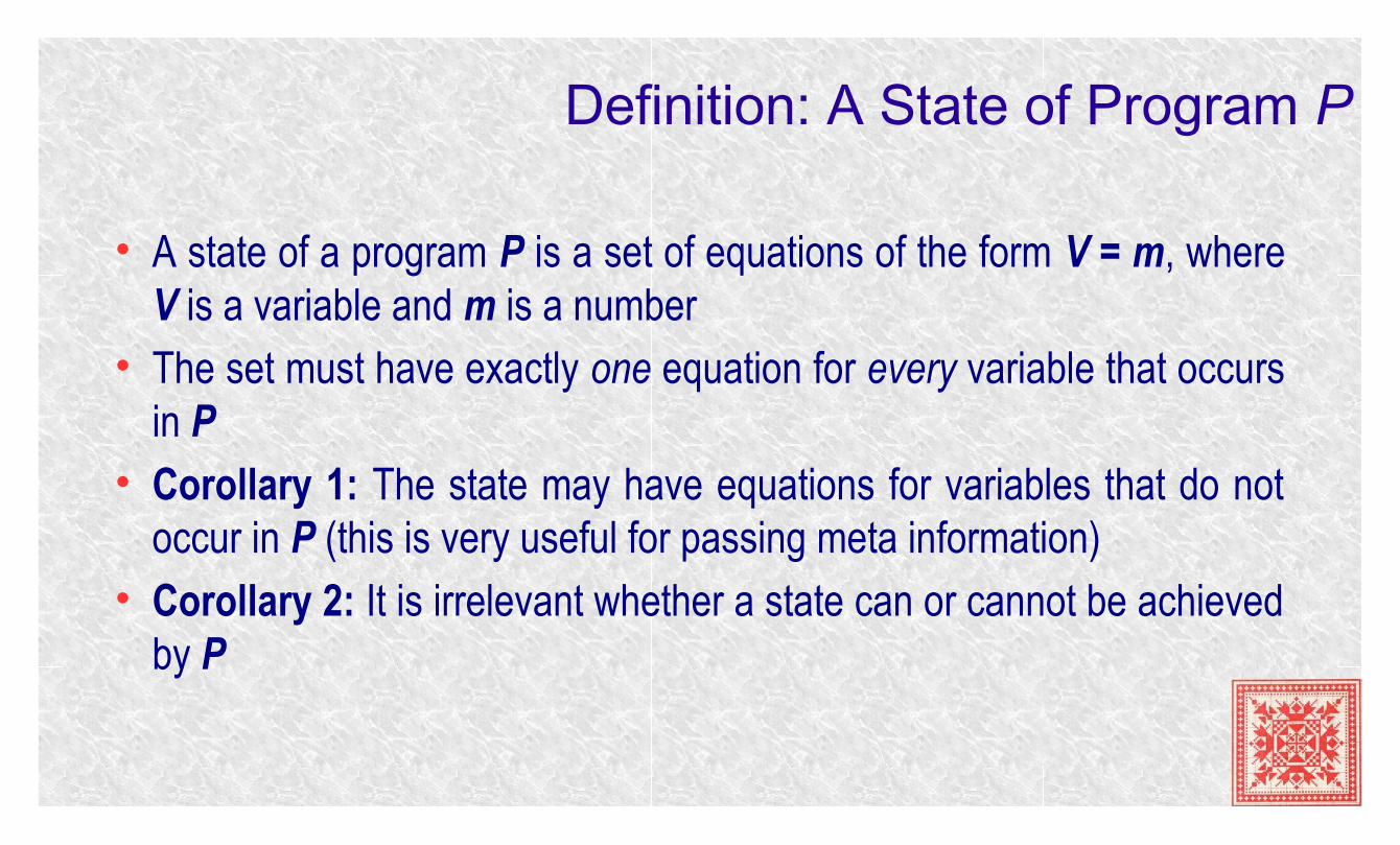
Definition: A State of Program P
• A state of a program P is a set of equations of the form V = m, where V is a variable and m is a number
• The set must have exactly one equation for every variable that occurs in P
• Corollary 1: The state may have equations for variables that do not occur in P (this is very useful for passing meta information)
• Corollary 2: It is irrelevant whether a state can or cannot be achieved by P
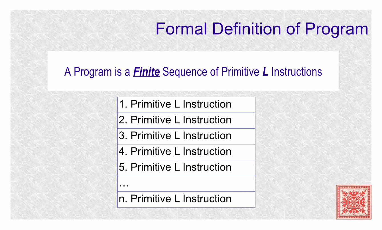
A Program is a Finite Sequence of Primitive L Instructions
1. Primitive L Instruction
2. Primitive L Instruction
3. Primitive L Instruction
4. Primitive L Instruction
5. Primitive L Instruction
…
n. Primitive L Instruction
Formal Definition of Program
Program Snapshots
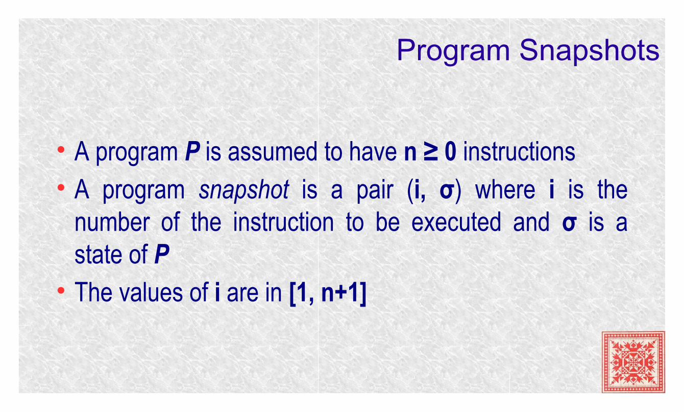
• A program P is assumed to have n ≥ 0 instructions• A program snapshot is a pair (i, σ) where i is the
number of the instruction to be executed and σ is a state of P
• The values of i are in [1, n+1]
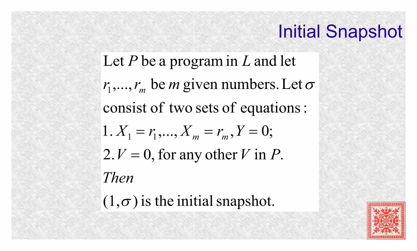
Initial Snapshot
snapshot. initial theis )(1,
.in other any for ,0 .2
;0,,..., 1.
:equations of sets twoofconsist
Let numbers.given be ,...,
let and in program a be Let
11
1
Then
PVV
YrXrX
mrr
LP
mm
m
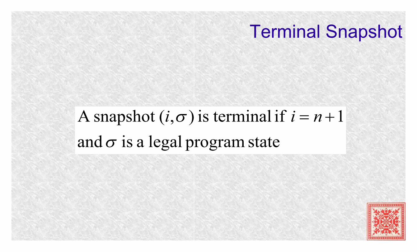
Terminal Snapshot
state program legal a is and
1 if terminalis ),(snapshot A
nii
Program Snapshot Sequences
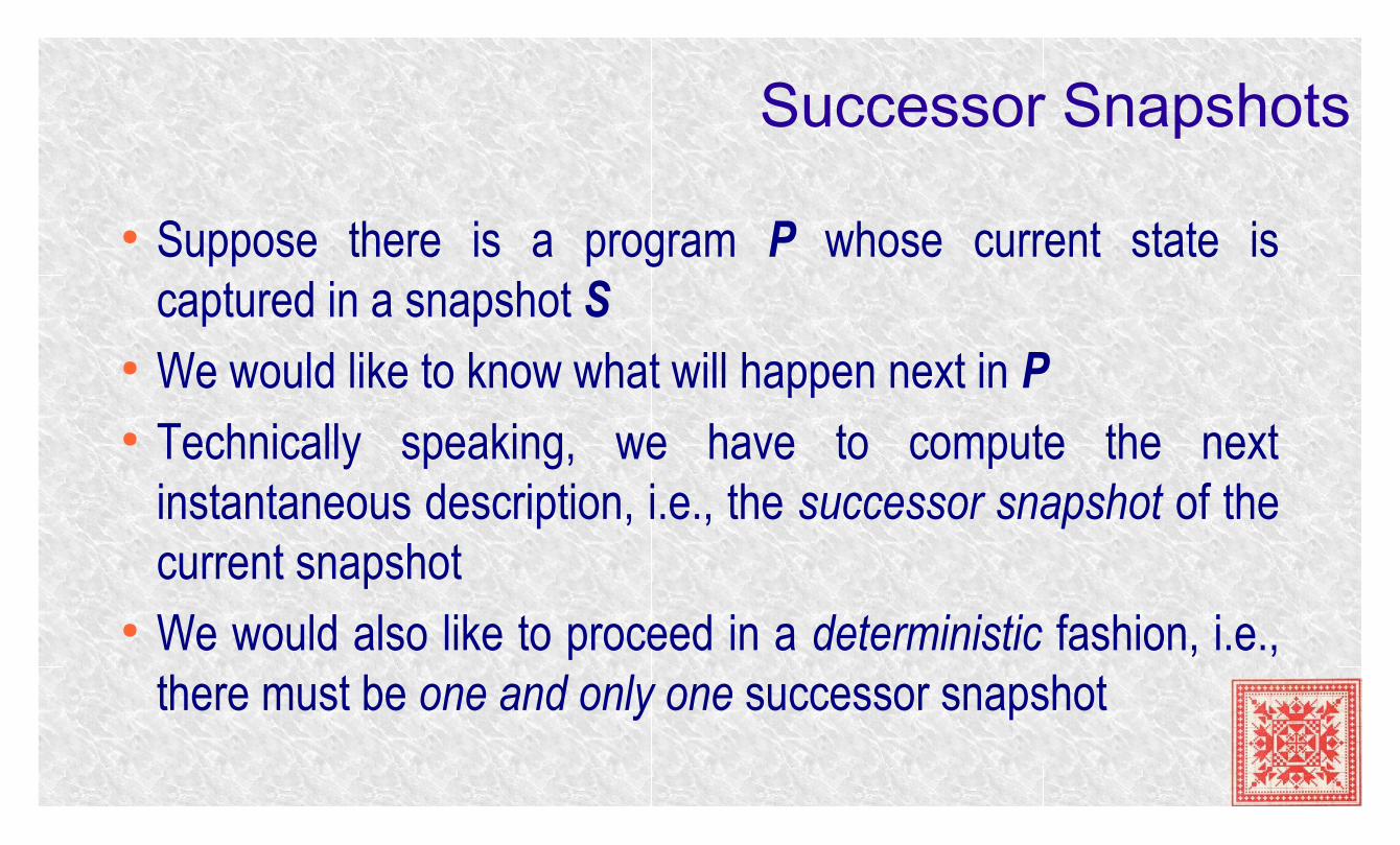
Successor Snapshots
● Suppose there is a program P whose current state is captured in a snapshot S
● We would like to know what will happen next in P ● Technically speaking, we have to compute the next
instantaneous description, i.e., the successor snapshot of the current snapshot
● We would also like to proceed in a deterministic fashion, i.e., there must be one and only one successor snapshot
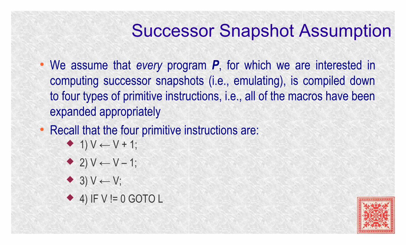
Successor Snapshot Assumption
● We assume that every program P, for which we are interested in computing successor snapshots (i.e., emulating), is compiled down to four types of primitive instructions, i.e., all of the macros have been expanded appropriately
● Recall that the four primitive instructions are: 1) V ← V + 1;
2) V ← V – 1;
3) V ← V;
4) IF V != 0 GOTO L
Successor Snapshots
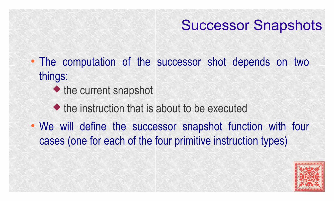
● The computation of the successor shot depends on two things:
the current snapshot the instruction that is about to be executed
● We will define the successor snapshot function with four cases (one for each of the four primitive instruction types)
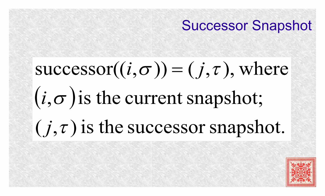
Successor Snapshot
snapshot.successor theis ),(
snapshot;current theis ,
where),,()),(successor(
j
i
ji
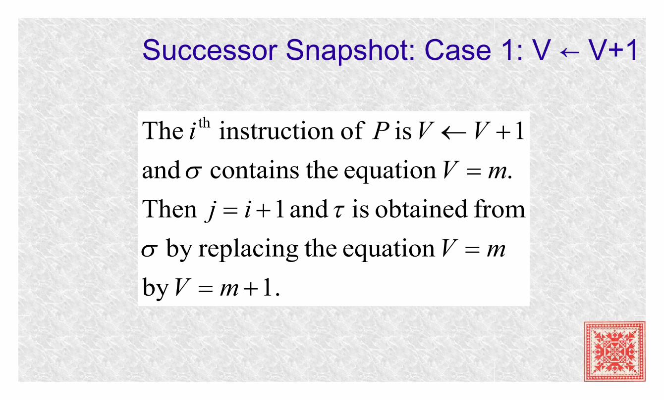
Successor Snapshot: Case 1: V ← V+1
.1by
equation thereplacingby
from obtained is and 1Then
.equation thecontains and
1 is ofn instructio The th
mV
mV
ij
mV
VVPi
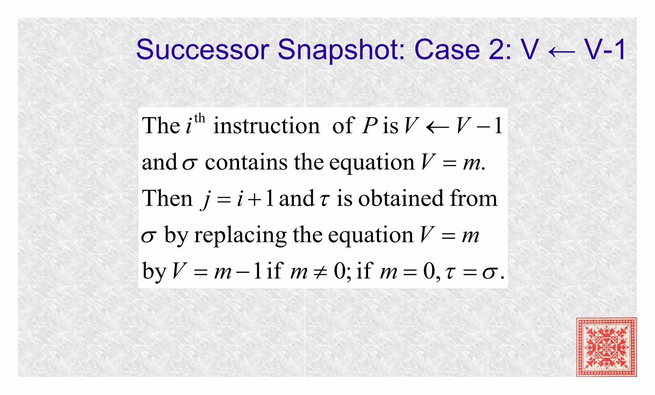
Successor Snapshot: Case 2: V ← V-1
. ,0 if ;0 if 1by
equation thereplacingby
from obtained is and 1Then
.equation thecontains and
1 is ofn instructio The th
mmmV
mV
ij
mV
VVPi
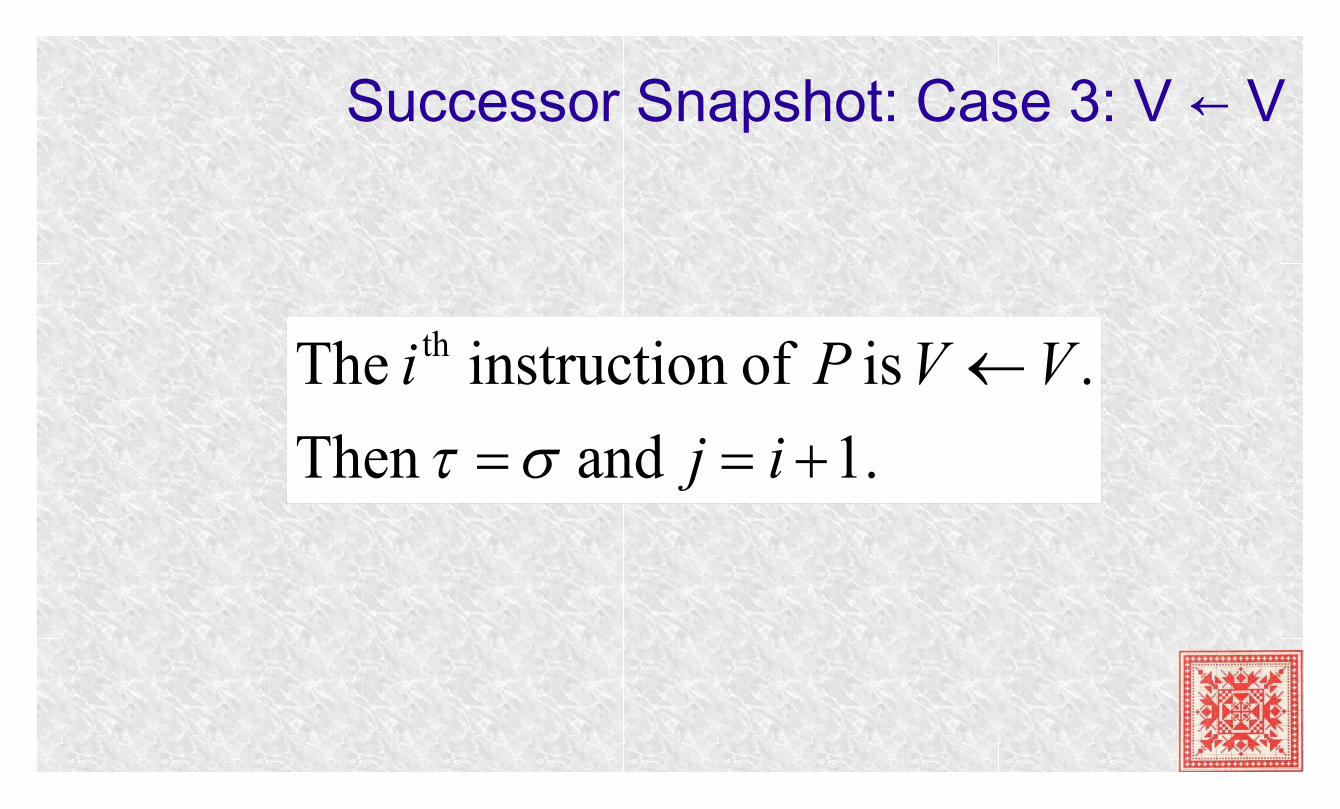
Successor Snapshot: Case 3: V ← V
.1 and Then
. is ofn instructio The th
ij
VVPi
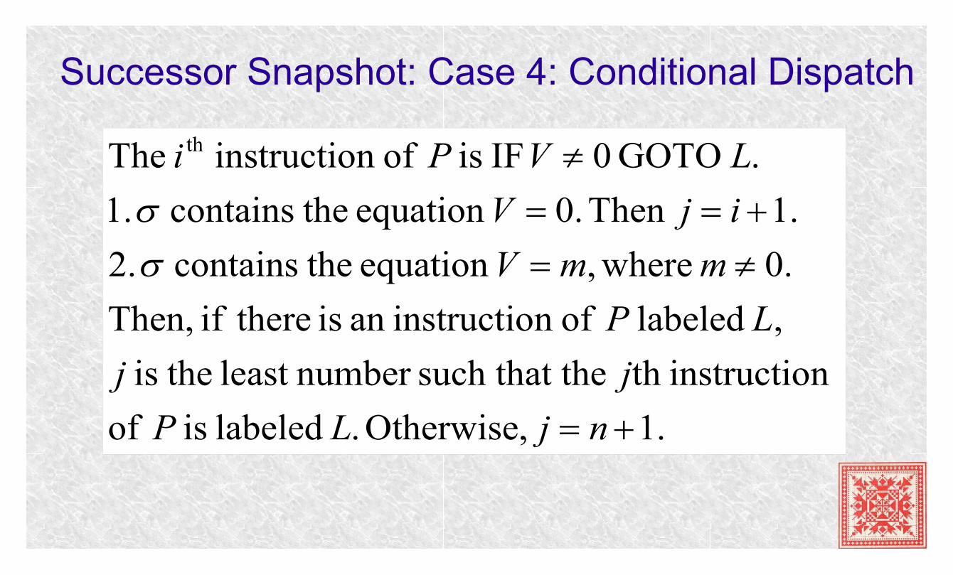
Successor Snapshot: Case 4: Conditional Dispatch
.1Otherwise, . labeled is of
n instructioth thesuch that number least theis
, labeled ofn instructioan is thereif Then,
.0 where,equation thecontains .2
.1Then .0equation thecontains .1
. GOTO 0 IF is ofn instructio The th
njLP
jj
LP
mmV
ijV
LVPi
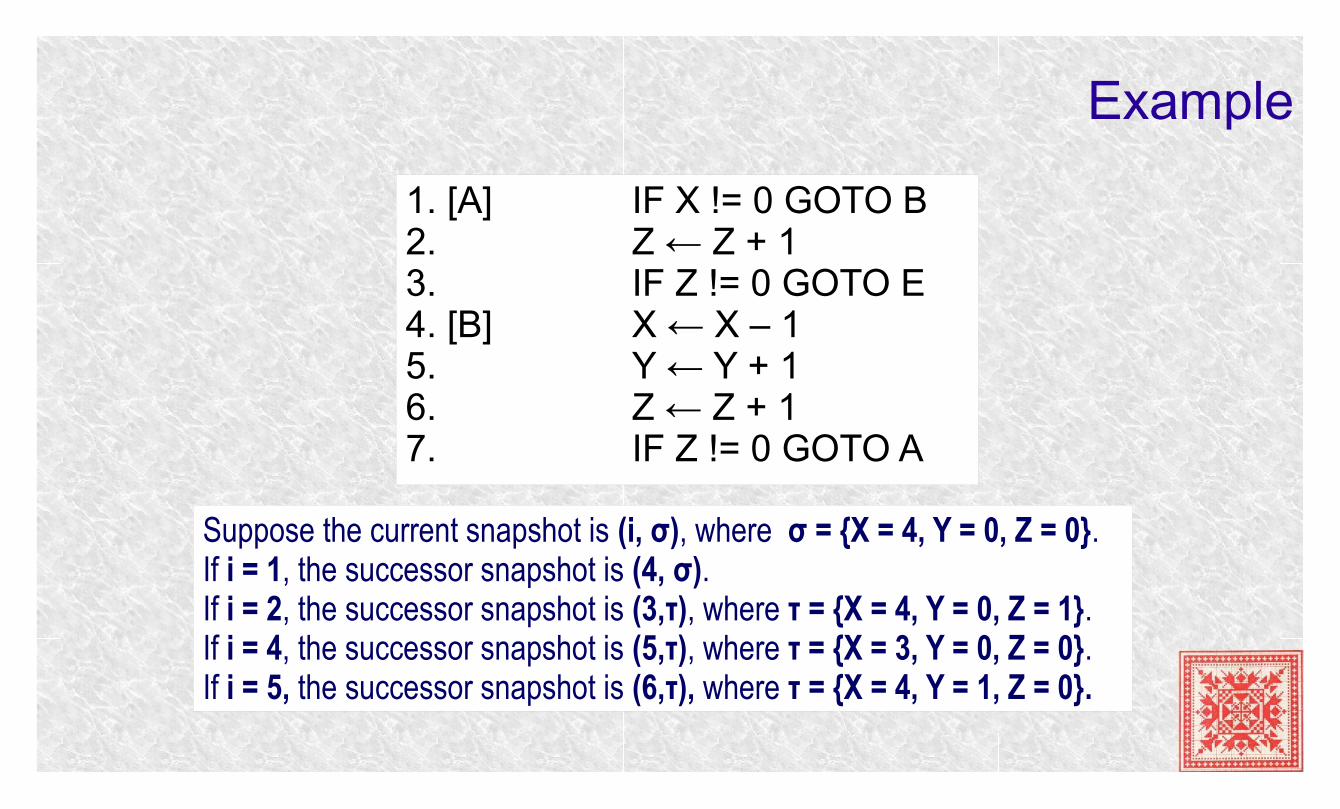
Example
1. [A] IF X != 0 GOTO B2. Z ← Z + 13. IF Z != 0 GOTO E4. [B] X ← X – 15. Y ← Y + 16. Z ← Z + 17. IF Z != 0 GOTO A
Suppose the current snapshot is (i, σ), where σ = {X = 4, Y = 0, Z = 0}. If i = 1, the successor snapshot is (4, σ).If i = 2, the successor snapshot is (3,τ), where τ = {X = 4, Y = 0, Z = 1}.If i = 4, the successor snapshot is (5,τ), where τ = {X = 3, Y = 0, Z = 0}.If i = 5, the successor snapshot is (6,τ), where τ = {X = 4, Y = 1, Z = 0}.
Computation
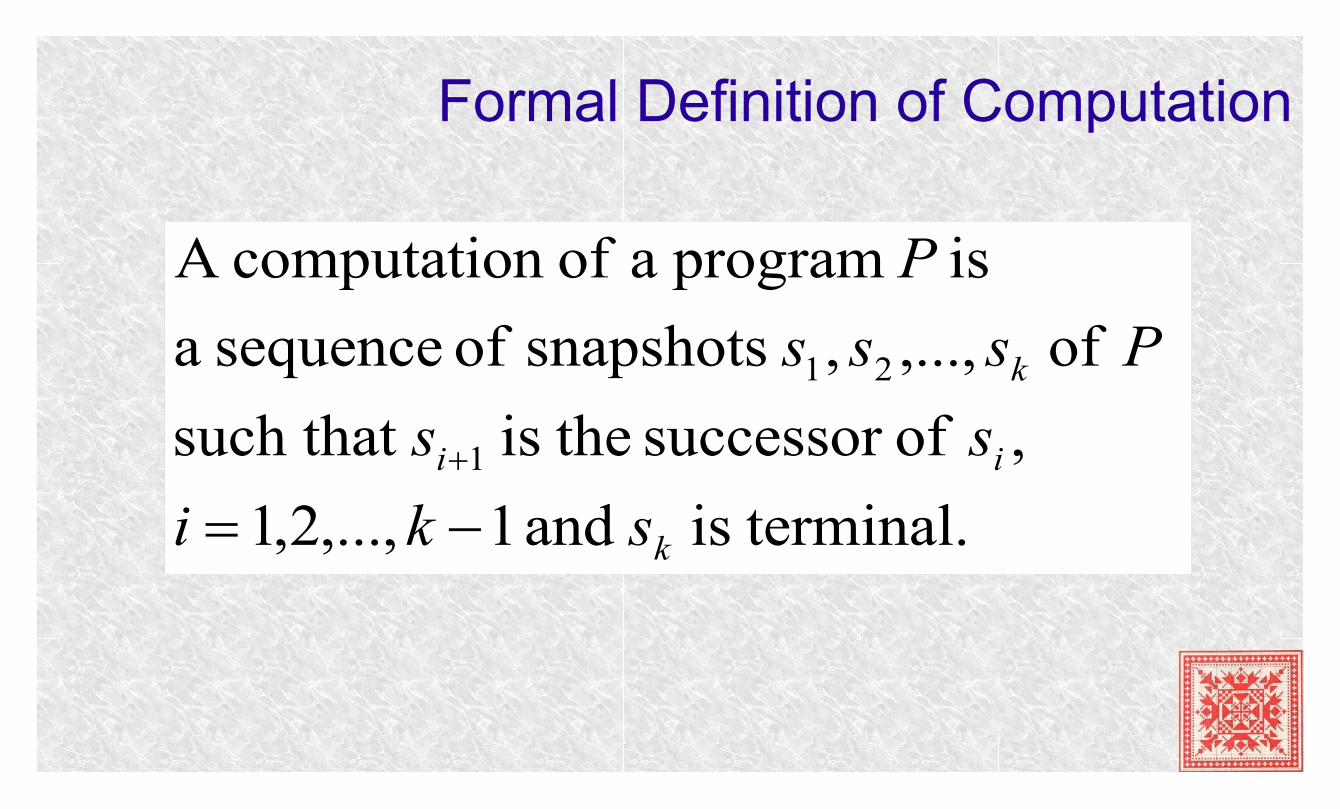
Formal Definition of Computation
terminal.is and 1,...,2,1
, ofsuccessor theis such that
of ,...,, snapshots of sequence a
is program a ofn computatioA
1
21
k
ii
k
ski
ss
Psss
P
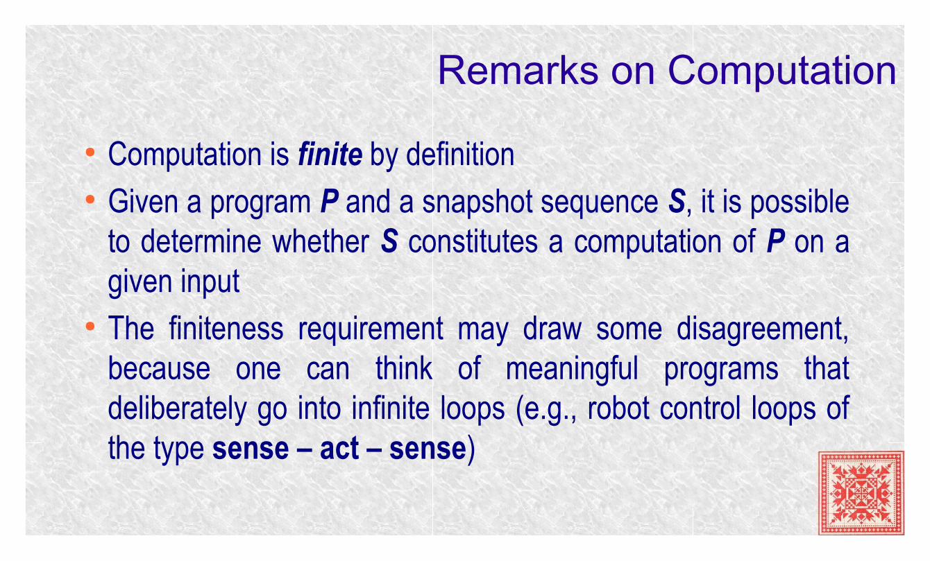
Remarks on Computation
● Computation is finite by definition● Given a program P and a snapshot sequence S, it is possible
to determine whether S constitutes a computation of P on a given input
● The finiteness requirement may draw some disagreement, because one can think of meaningful programs that deliberately go into infinite loops (e.g., robot control loops of the type sense – act – sense)
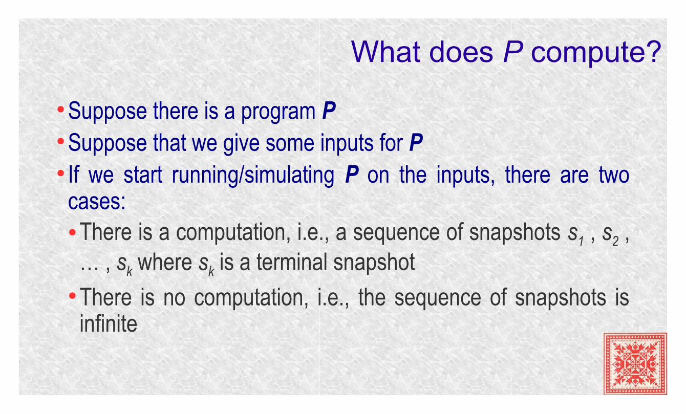
What does P compute?
● Suppose there is a program P● Suppose that we give some inputs for P● If we start running/simulating P on the inputs, there are two
cases:● There is a computation, i.e., a sequence of snapshots s1 , s2 ,
… , sk where sk is a terminal snapshot● There is no computation, i.e., the sequence of snapshots is
infinite
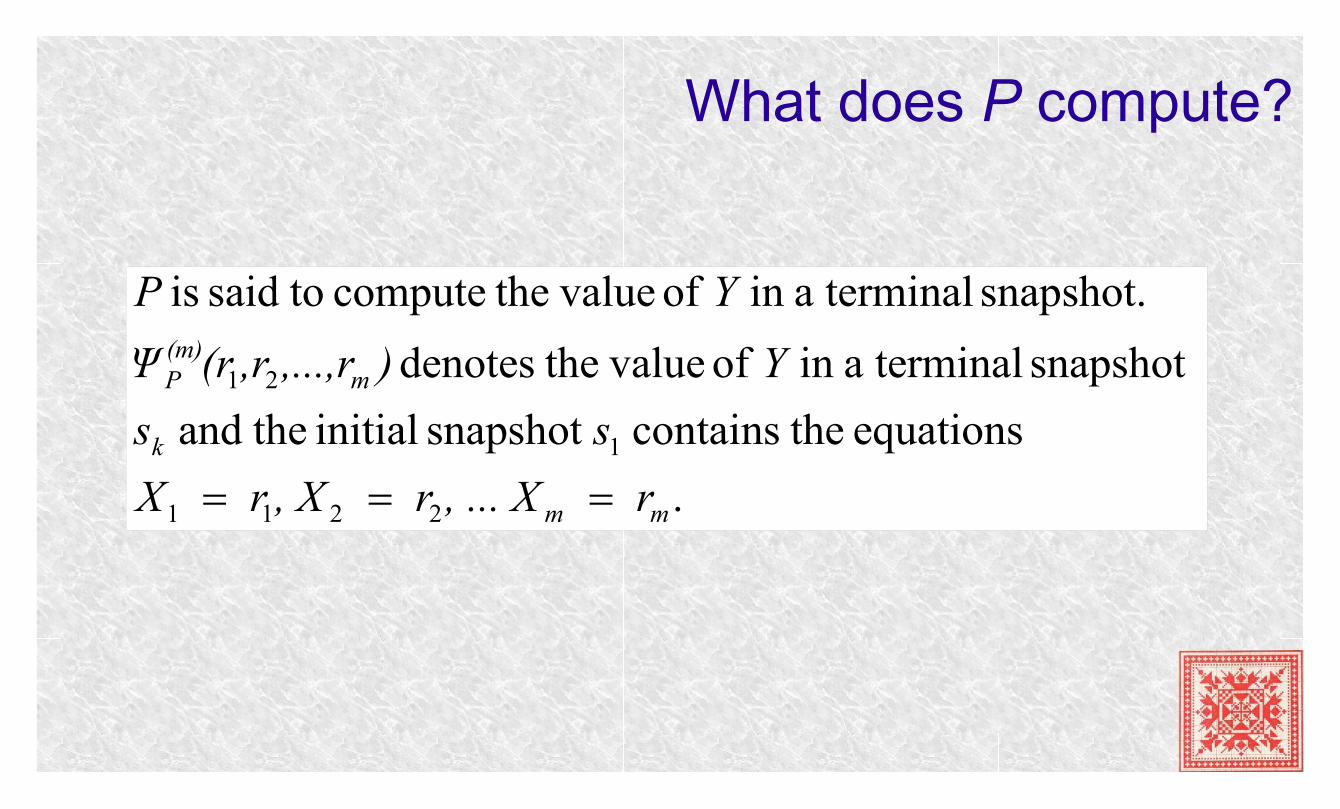
What does P compute?
.
equations thecontains snapshot initial theand
snapshot terminalain of value thedenotes
snapshot. terminalain of value thecompute tosaid is
2211
1
21
mm
k
m(m)P
r , ... X r , X r X
ss
Y),...,r,r(rΨ
YP
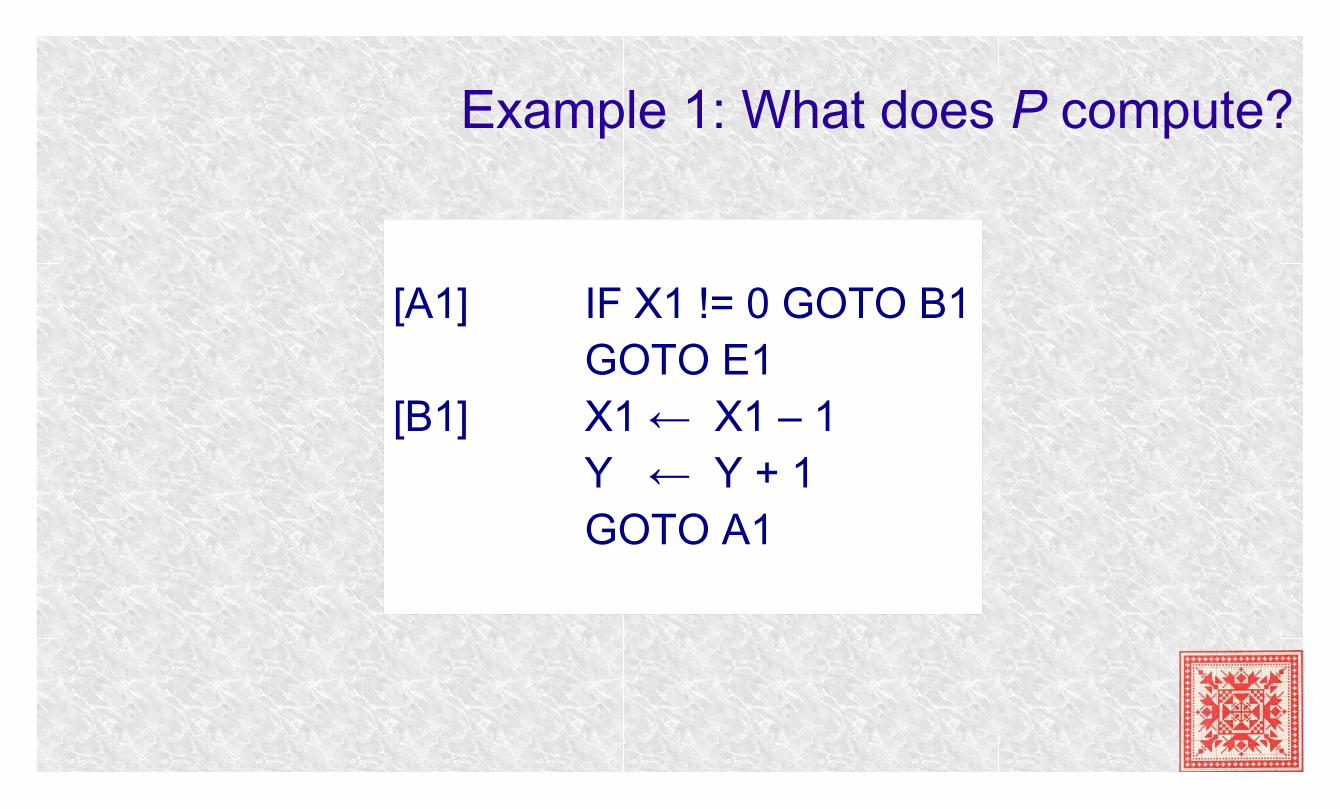
Example 1: What does P compute?
[A1] IF X1 != 0 GOTO B1GOTO E1
[B1] X1 ← X1 – 1Y ← Y + 1GOTO A1
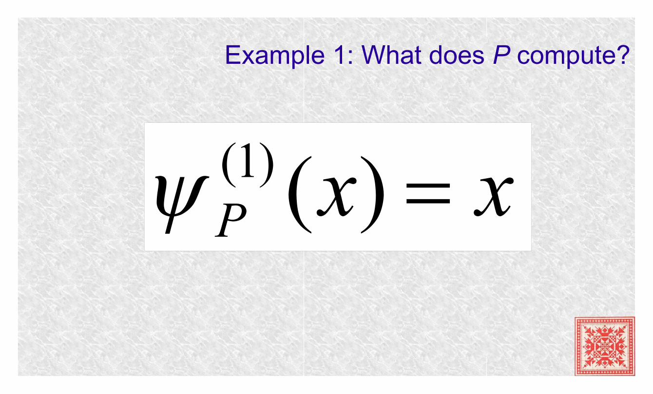
Example 1: What does P compute?
xxP )()1(
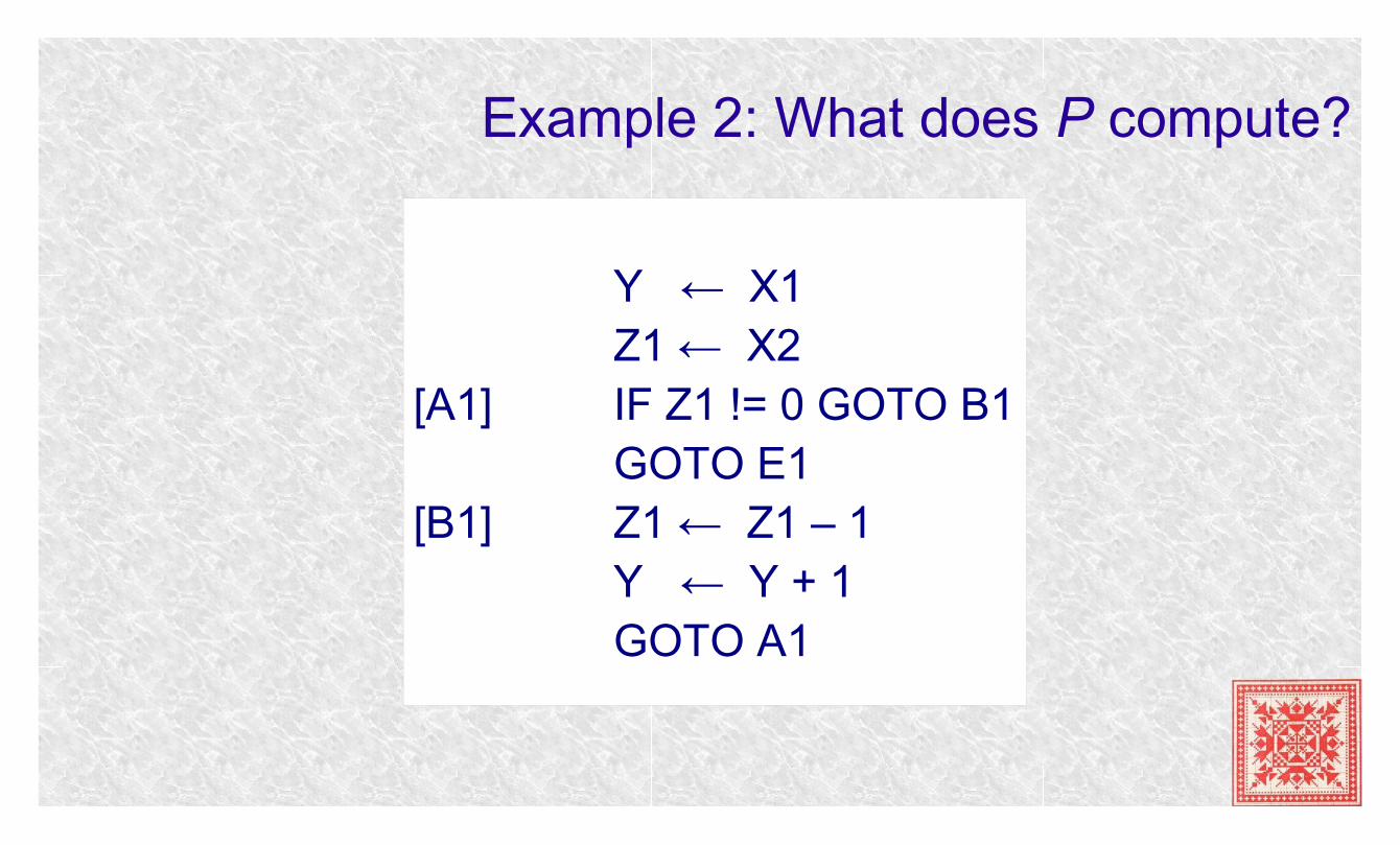
Example 2: What does P compute?
Y ← X1Z1 ← X2
[A1] IF Z1 != 0 GOTO B1GOTO E1
[B1] Z1 ← Z1 – 1Y ← Y + 1GOTO A1
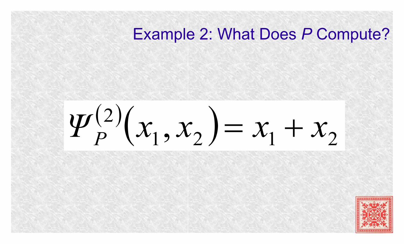
Example 2: What Does P Compute?
21212 , xxxxΨ P
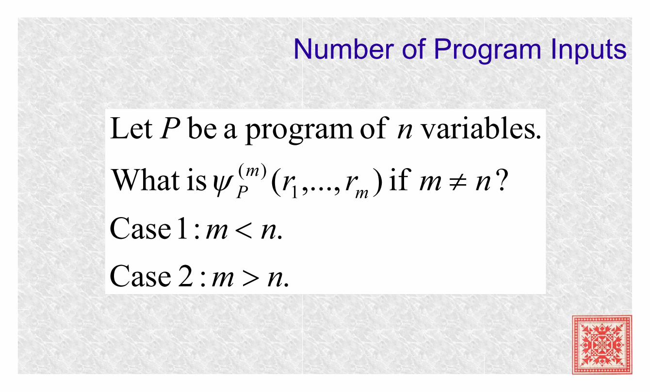
Number of Program Inputs
. :2 Case
. :1 Case
? if ),...,( isWhat
. variables of program a be Let
1)(
nm
nm
nmrr
nP
mm
P
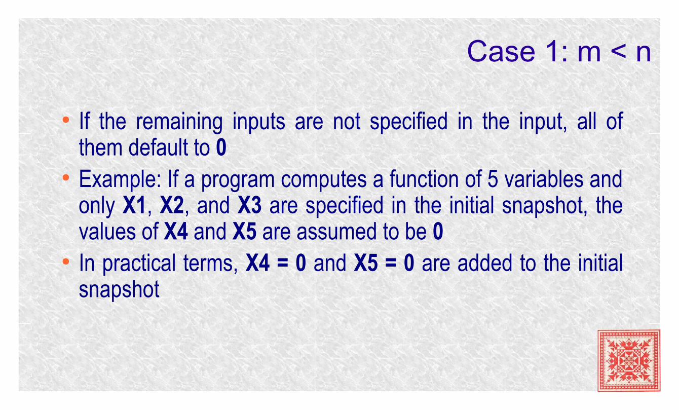
Case 1: m < n
● If the remaining inputs are not specified in the input, all of them default to 0
● Example: If a program computes a function of 5 variables and only X1, X2, and X3 are specified in the initial snapshot, the values of X4 and X5 are assumed to be 0
● In practical terms, X4 = 0 and X5 = 0 are added to the initial snapshot
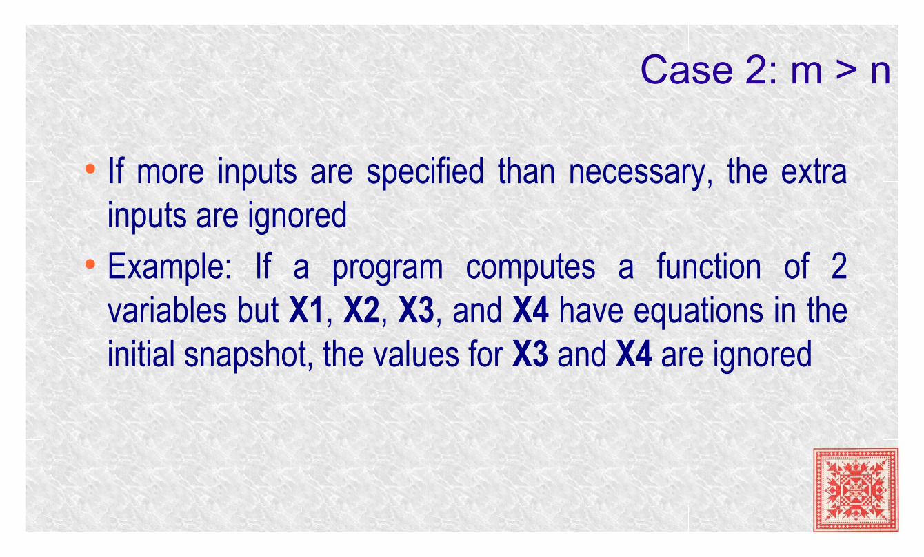
Case 2: m > n
● If more inputs are specified than necessary, the extra inputs are ignored
● Example: If a program computes a function of 2 variables but X1, X2, X3, and X4 have equations in the initial snapshot, the values for X3 and X4 are ignored
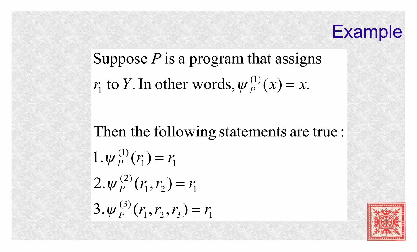
Example
1321)3(
121)2(
11)1(
)1(1
),,( .3
),( .2
)( .1
: trueare statements following Then the
.)( s,other wordIn . to
assigns that program a is Suppose
rrrr
rrr
rr
xxYr
P
P
P
P
P
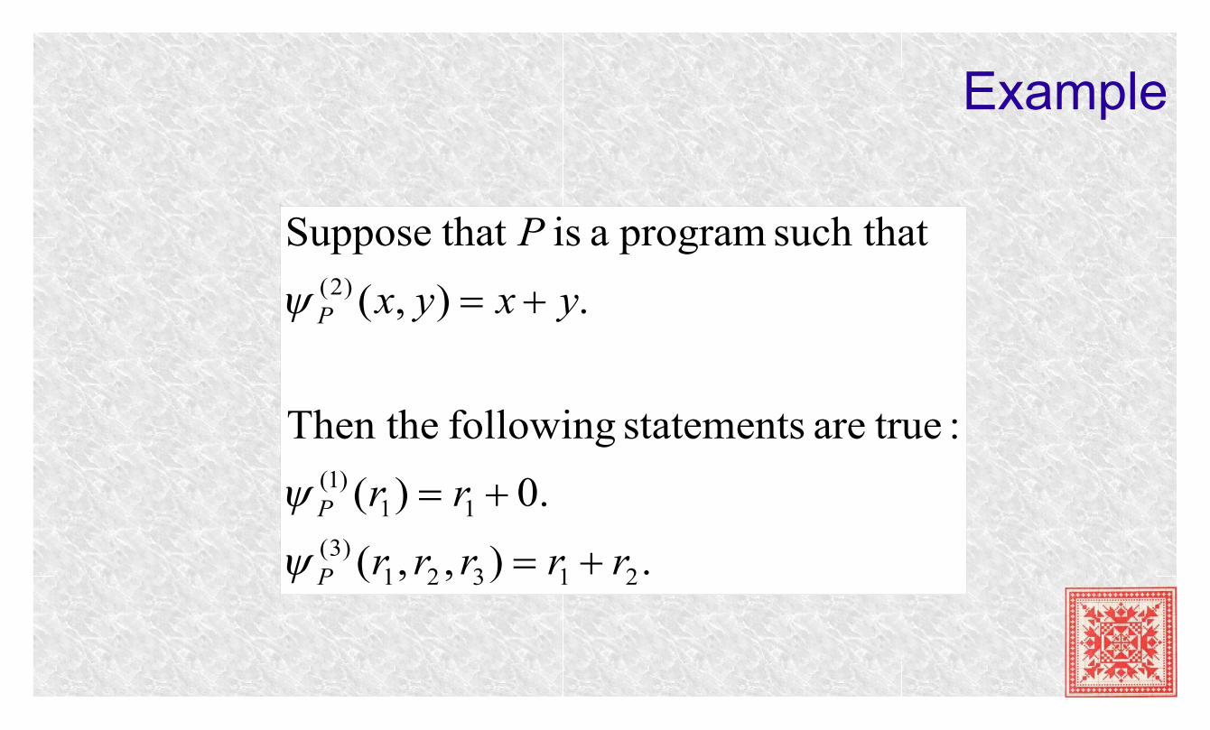
Example
.),,(
.0)(
: trueare statements following Then the
.),(
such that program a is that Suppose
21321)3(
11)1(
)2(
rrrrr
rr
yxyx
P
P
P
P
Partially Computable Functions&
Computable Functions
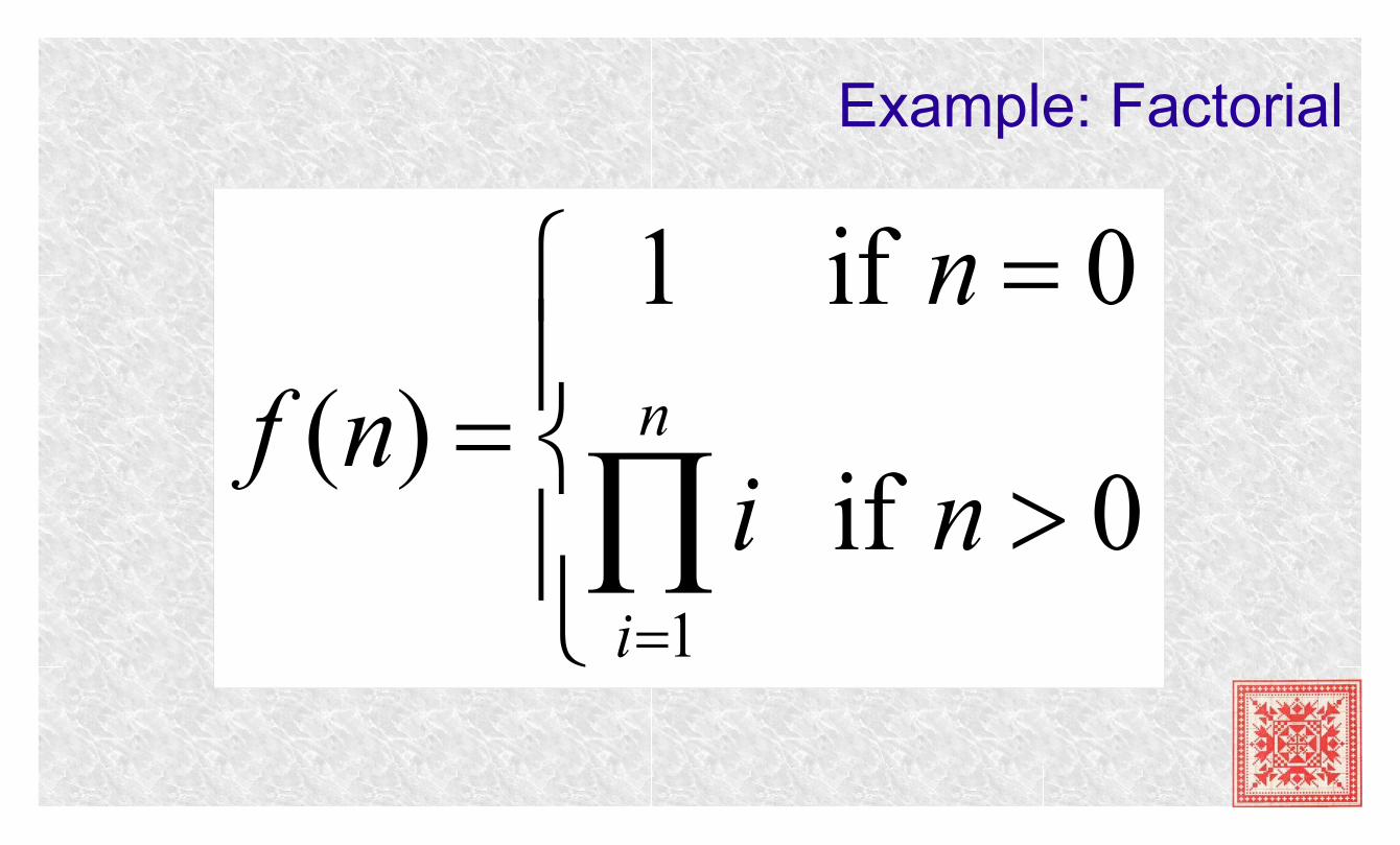
Example: Factorial
0 if
0 if 1
)(
1
ni
n
nf n
i
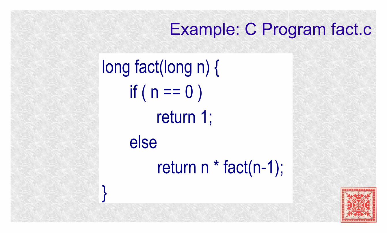
Example: C Program fact.c
long fact(long n) {if ( n == 0 )
return 1;else
return n * fact(n-1);}
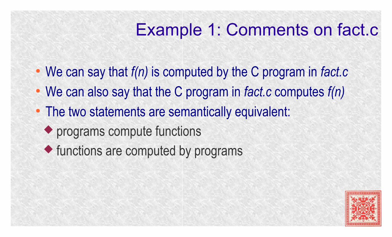
Example 1: Comments on fact.c
● We can say that f(n) is computed by the C program in fact.c● We can also say that the C program in fact.c computes f(n)● The two statements are semantically equivalent:
programs compute functions functions are computed by programs
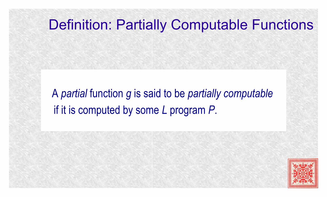
Definition: Partially Computable Functions
A partial function g is said to be partially computable
if it is computed by some L program P.
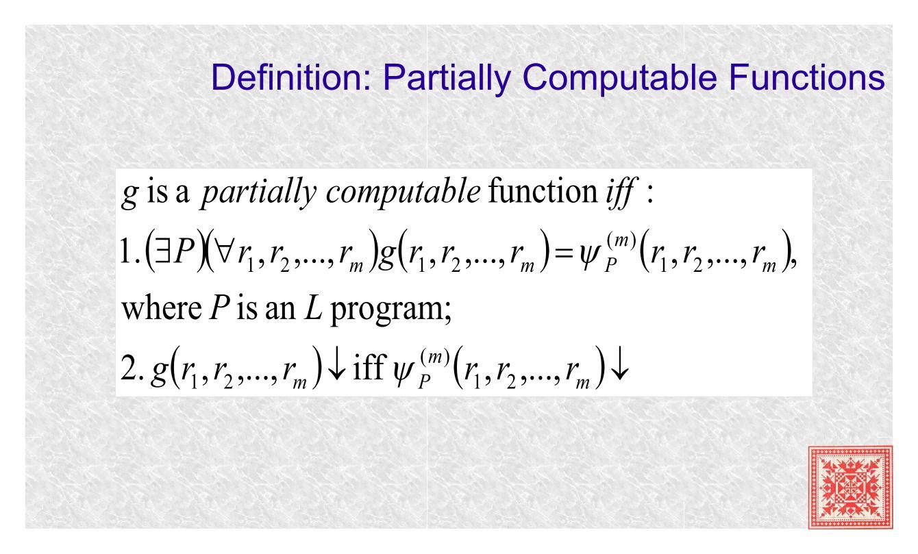
Definition: Partially Computable Functions
mm
Pm
mm
Pmm
rrrrrrg
LP
rrrrrrgrrrP
iffcomputablepartially g
,...,, iff ,...,, .2
program; an is where
,,...,,,...,,,...,, .1
:function a is
21)(
21
21)(
2121
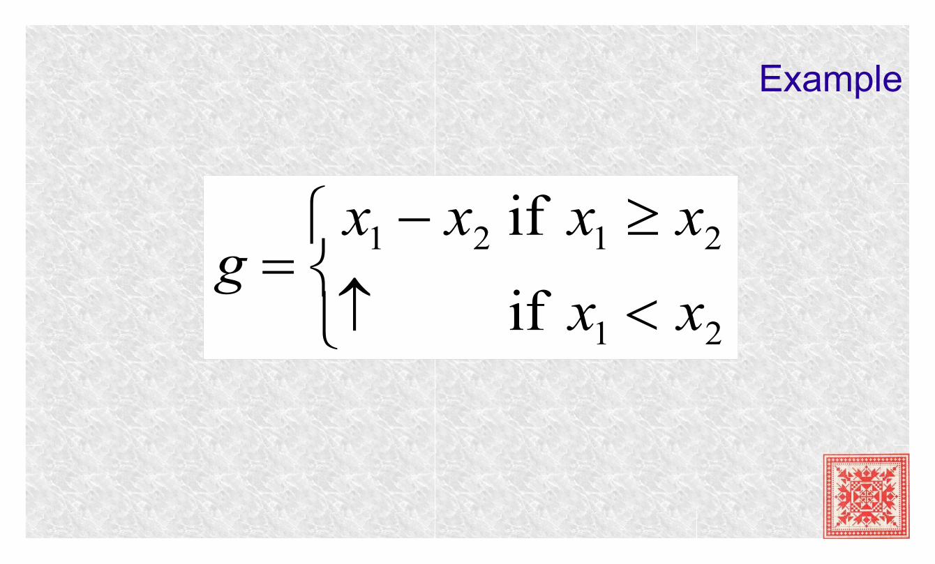
Example
21
2121
if
if
xx
xxxxg
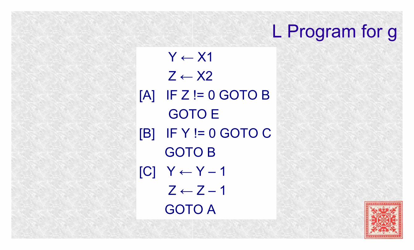
L Program for g Y ← X1
Z ← X2
[A] IF Z != 0 GOTO B
GOTO E
[B] IF Y != 0 GOTO C
GOTO B
[C] Y ← Y – 1
Z ← Z – 1
GOTO A
Example
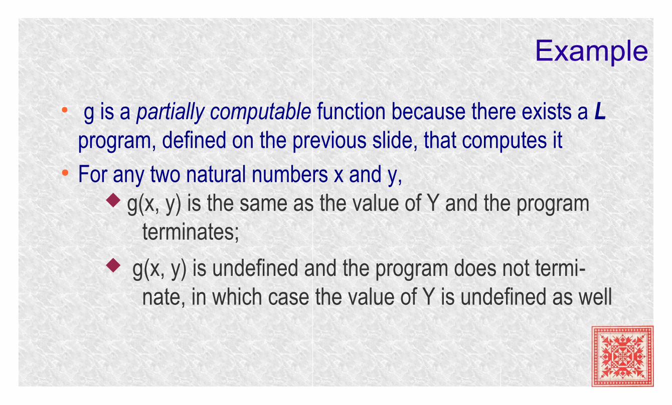
● g is a partially computable function because there exists a L program, defined on the previous slide, that computes it
● For any two natural numbers x and y, g(x, y) is the same as the value of Y and the program
terminates; g(x, y) is undefined and the program does not termi-
nate, in which case the value of Y is undefined as well
Definition: Computable Functions
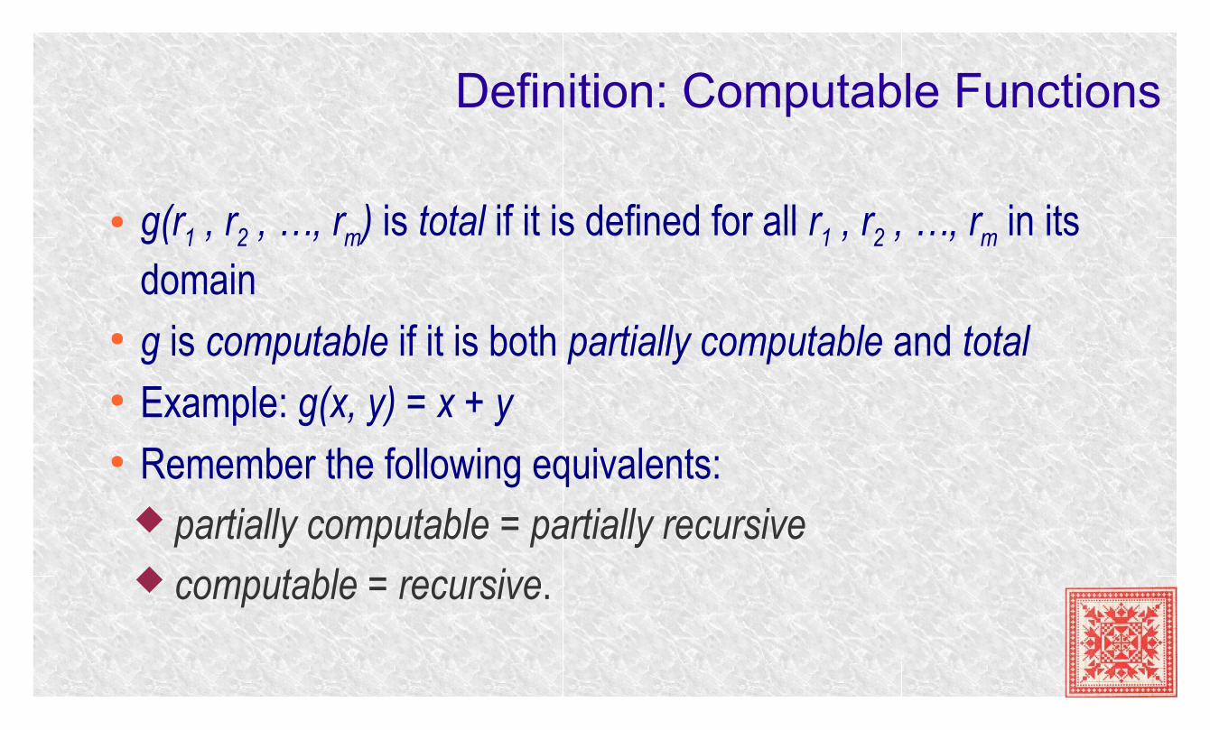
● g(r1 , r2 , …, rm) is total if it is defined for all r1 , r2 , …, rm in its domain
● g is computable if it is both partially computable and total● Example: g(x, y) = x + y● Remember the following equivalents:
partially computable = partially recursive computable = recursive.
Partially Computable vs. Computable Functions
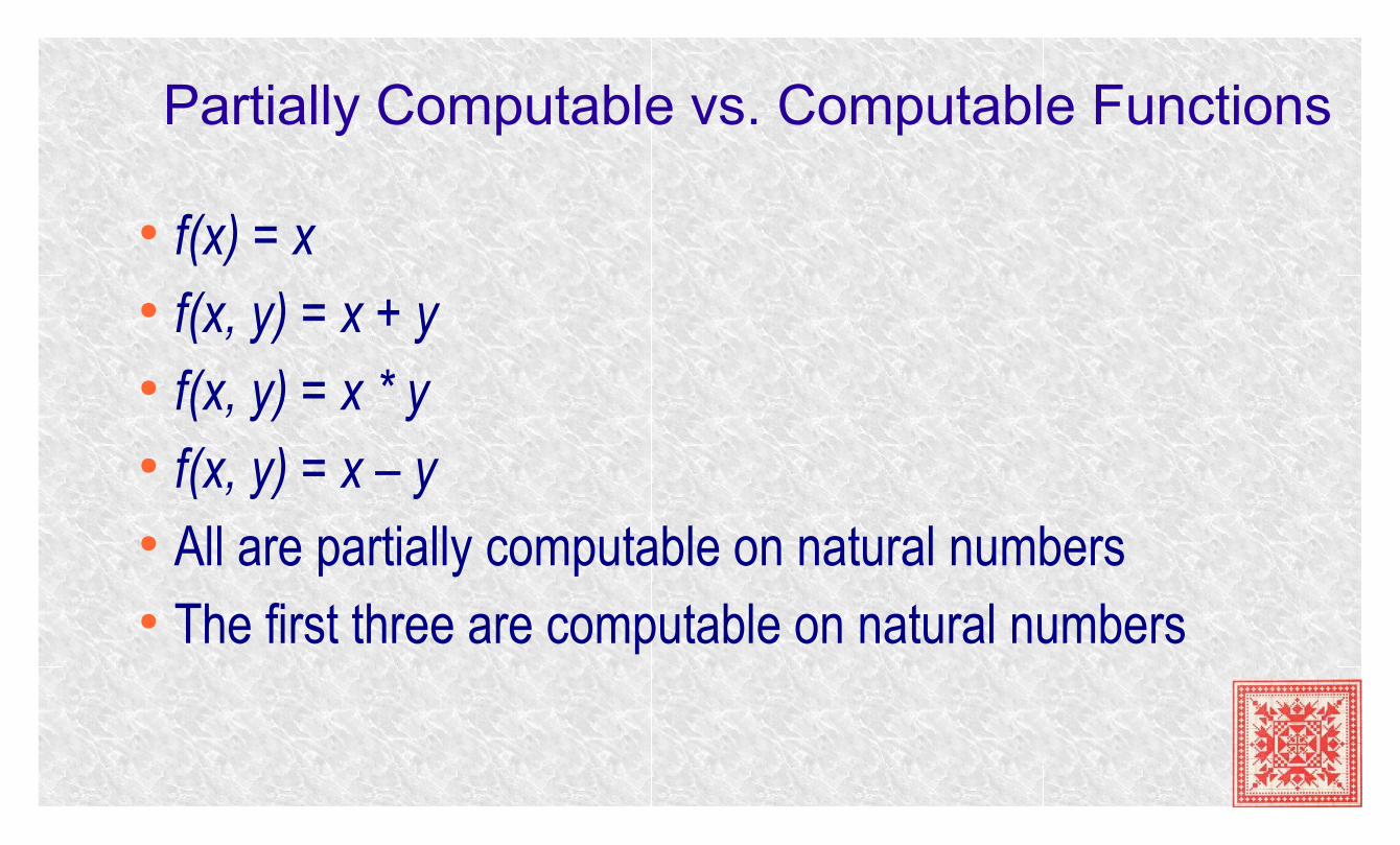
● f(x) = x● f(x, y) = x + y● f(x, y) = x * y● f(x, y) = x – y● All are partially computable on natural numbers● The first three are computable on natural numbers
Function Macros & Their Expansion
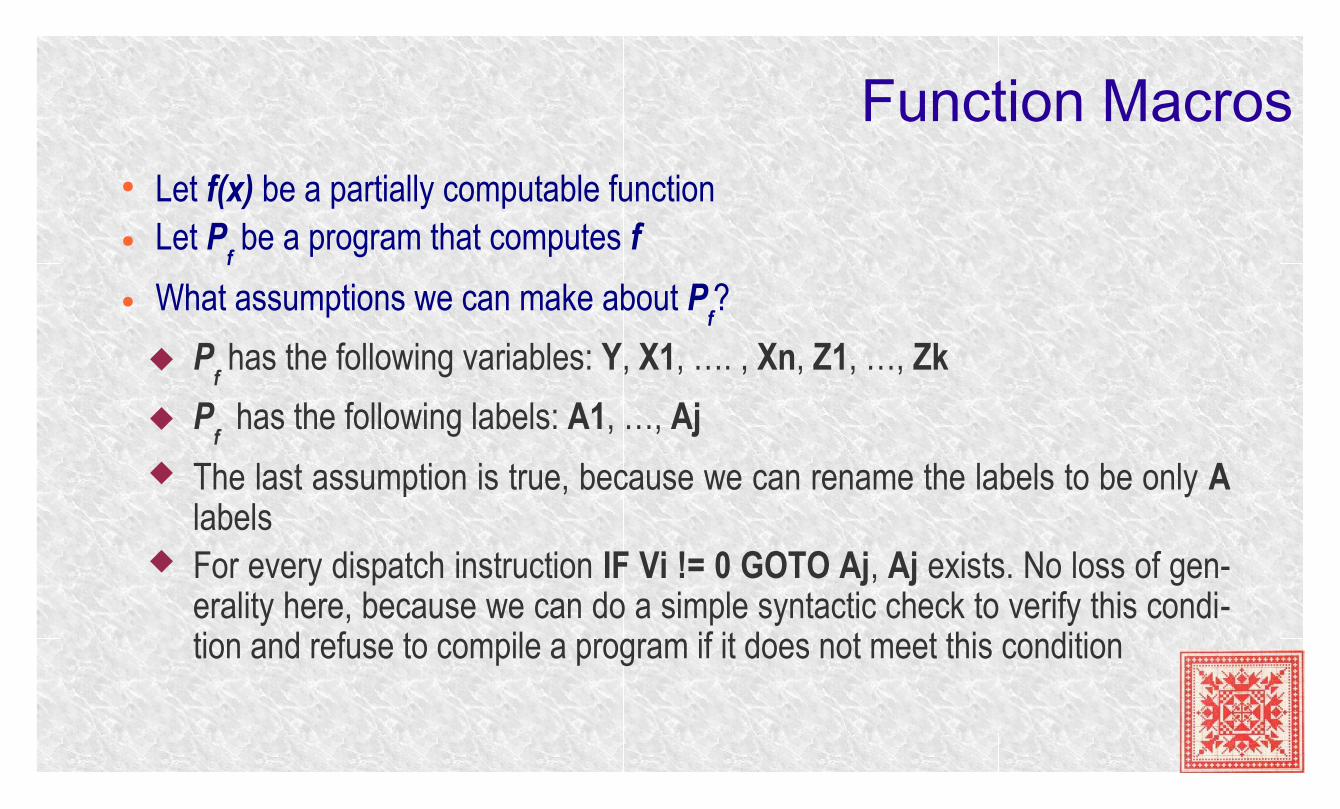
Function Macros● Let f(x) be a partially computable function● Let P
f be a program that computes f
● What assumptions we can make about Pf?
Pf has the following variables: Y, X1, …. , Xn, Z1, …, Zk
Pf has the following labels: A1, …, Aj
The last assumption is true, because we can rename the labels to be only A labels
For every dispatch instruction IF Vi != 0 GOTO Aj, Aj exists. No loss of gen-erality here, because we can do a simple syntactic check to verify this condi-tion and refuse to compile a program if it does not meet this condition
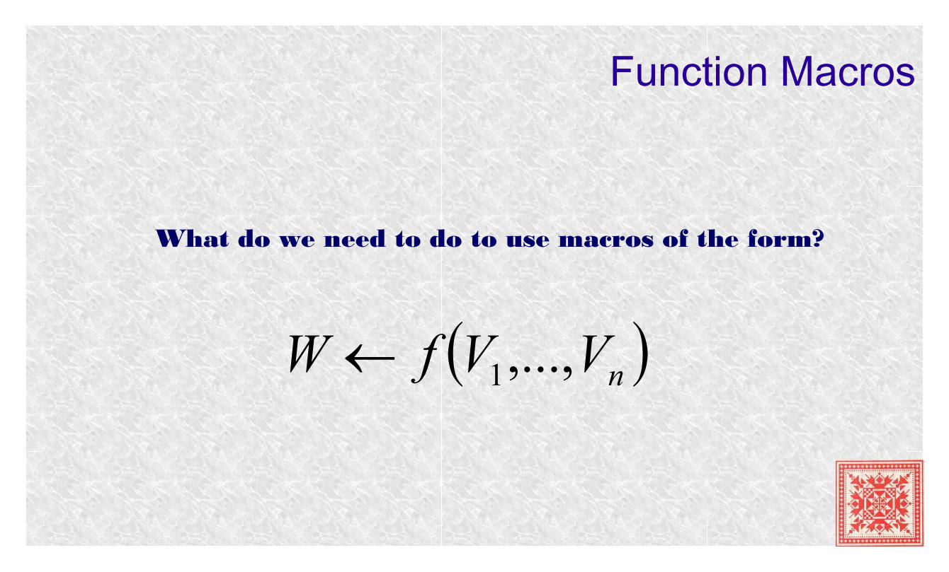
Function Macros
What do we need to do to use macros of the form?
nVVfW ,..., 1
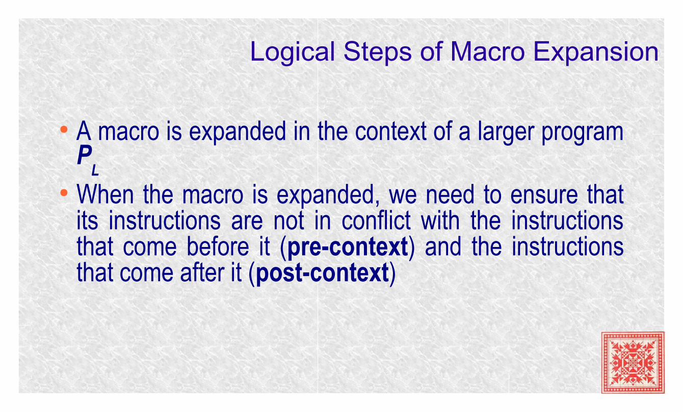
Logical Steps of Macro Expansion
● A macro is expanded in the context of a larger program P
L● When the macro is expanded, we need to ensure that
its instructions are not in conflict with the instructions that come before it (pre-context) and the instructions that come after it (post-context)
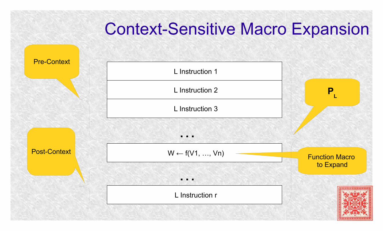
Context-Sensitive Macro Expansion
L Instruction 1
L Instruction 2
L Instruction 3
L Instruction r
W ← f(V1, …, Vn)
…
…
Pre-Context
Post-ContextFunction Macro
to Expand
PL
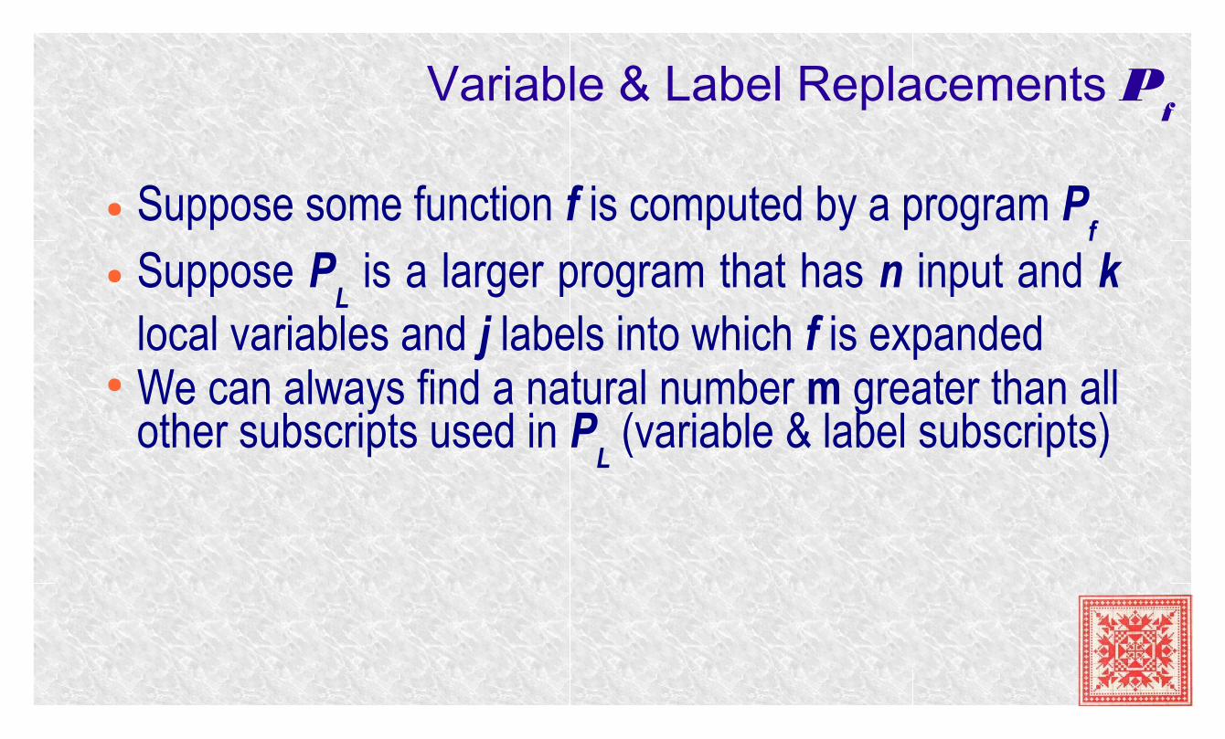
Variable & Label Replacements Pf
● Suppose some function f is computed by a program Pf
● Suppose PL is a larger program that has n input and k
local variables and j labels into which f is expanded● We can always find a natural number m greater than all
other subscripts used in PL (variable & label subscripts)
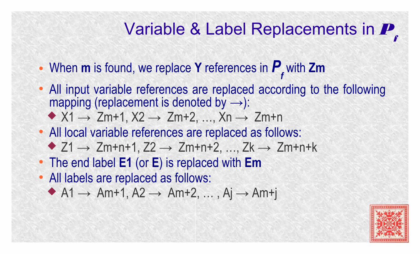
Variable & Label Replacements in Pf
● When m is found, we replace Y references in Pf with Zm
● All input variable references are replaced according to the following mapping (replacement is denoted by →): X1 → Zm+1, X2 → Zm+2, …, Xn → Zm+n
● All local variable references are replaced as follows: Z1 → Zm+n+1, Z2 → Zm+n+2, …, Zk → Zm+n+k
● The end label E1 (or E) is replaced with Em● All labels are replaced as follows:
A1 → Am+1, A2 → Am+2, … , Aj → Am+j
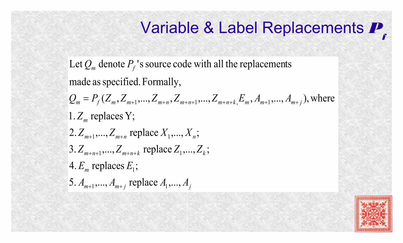
Variable & Label Replacements Pf
jjmm
m
kknmnm
nnmm
m
jmmmknmnmnmmmfm
fm
AAAA
EE
ZZZZ
XXZZ
Z
AAEZZZZZPQ
PQ
,..., replace ,..., .5
; replaces .4
;,..., replace ,..., .3
;,..., replace ,..., .2
Y; replaces .1
where),,...,,,...,,,...,,(
Formally, specified. as made
tsreplacemen theall with code source s' denote Let
11
1
11
11
1,11
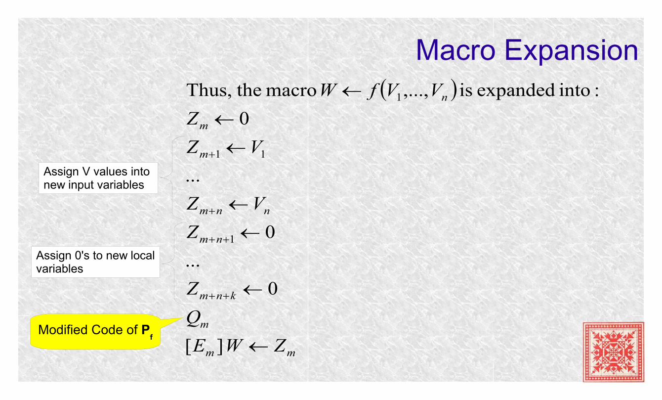
Macro Expansion
mm
m
knm
nm
nnm
m
m
n
ZWE
Q
Z
Z
VZ
VZ
Z
VVfW
][
0
...
0
...
0
:into expanded is ,..., macro theThus,
1
11
1
Assign V values into new input variables
Assign 0's to new localvariables
Modified Code of Pf
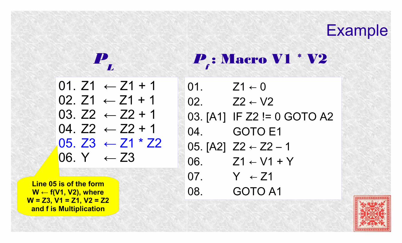
Example
01. Z1 ← Z1 + 102. Z1 ← Z1 + 103. Z2 ← Z2 + 104. Z2 ← Z2 + 105. Z3 ← Z1 * Z206. Y ← Z3
PL
01. Z1 ← 002. Z2 ← V203. [A1] IF Z2 != 0 GOTO A204. GOTO E105. [A2] Z2 ← Z2 – 106. Z1 ← V1 + Y07. Y ← Z108. GOTO A1
Pf : Macro V1 * V2
Line 05 is of the formW ← f(V1, V2), where
W = Z3, V1 = Z1, V2 = Z2and f is Multiplication
Example
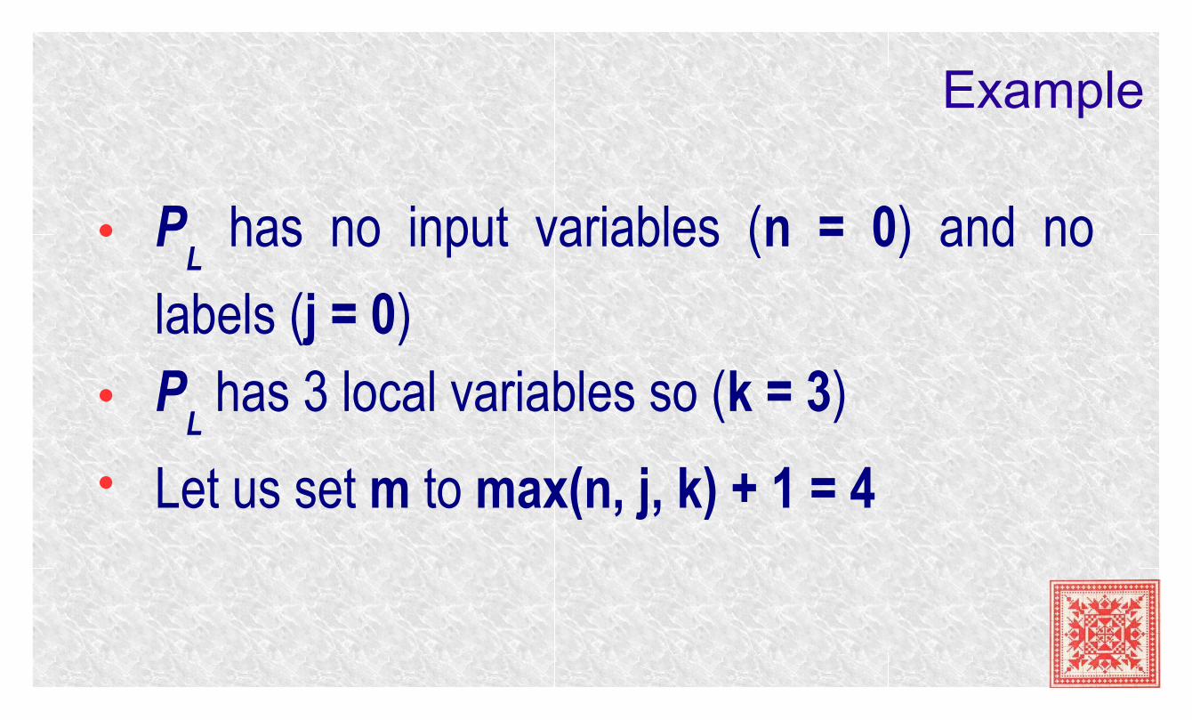
• PL
has no input variables (n = 0) and no
labels (j = 0)• P
L has 3 local variables so (k = 3)
• Let us set m to max(n, j, k) + 1 = 4
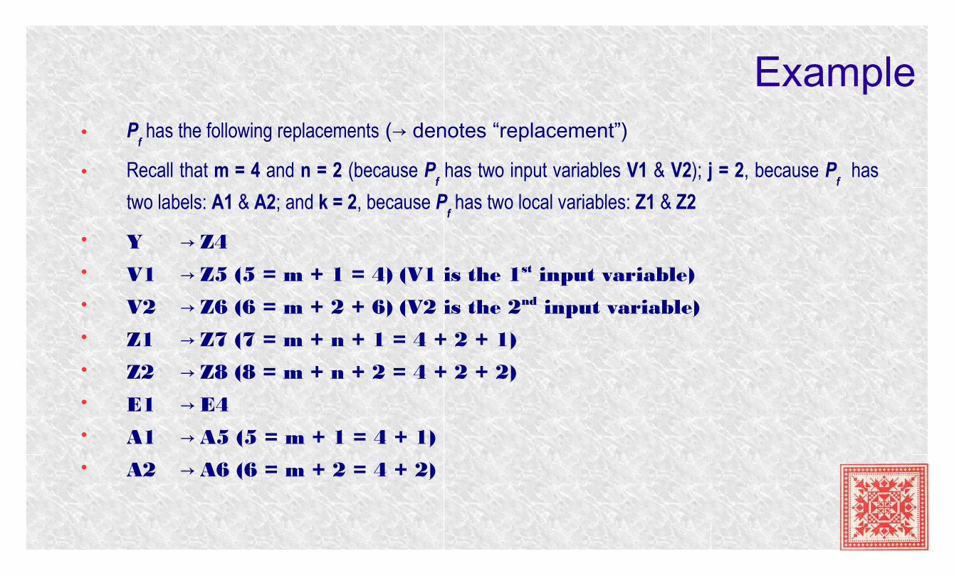
Example• P
f has the following replacements (→ denotes “replacement”)
• Recall that m = 4 and n = 2 (because Pf has two input variables V1 & V2); j = 2, because P
f has
two labels: A1 & A2; and k = 2, because Pf has two local variables: Z1 & Z2
• Y Z4→• V1 Z5 (5 = m + 1 = 4) (V1 is the 1→ st input variable)• V2 Z6 (6 = m + 2 + 6) (V2 is the 2→ nd input variable)• Z1 Z7 (7 = m + n + 1 = 4 + 2 + 1)→• Z2 Z8 (8 = m + n + 2 = 4 + 2 + 2)→• E1 E4→• A1 A5 (5 = m + 1 = 4 + 1)→• A2 A6 (6 = m + 2 = 4 + 2)→
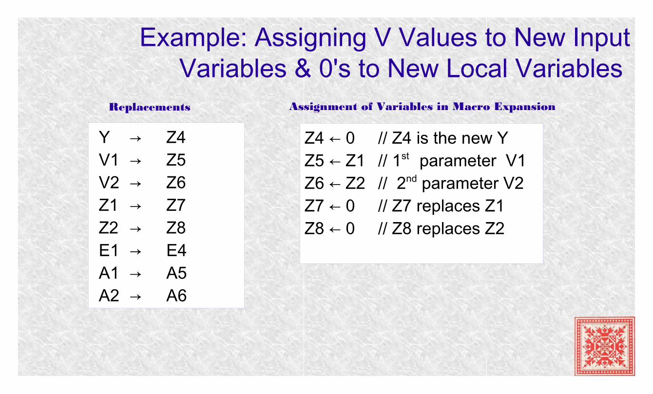
Example: Assigning V Values to New Input Variables & 0's to New Local Variables
Replacements
Z4 ← 0 // Z4 is the new YZ5 ← Z1 // 1st parameter V1Z6 ← Z2 // 2nd parameter V2Z7 ← 0 // Z7 replaces Z1Z8 ← 0 // Z8 replaces Z2
Assignment of Variables in Macro Expansion Y → Z4V1 → Z5 V2 → Z6 Z1 → Z7 Z2 → Z8 E1 → E4A1 → A5 A2 → A6
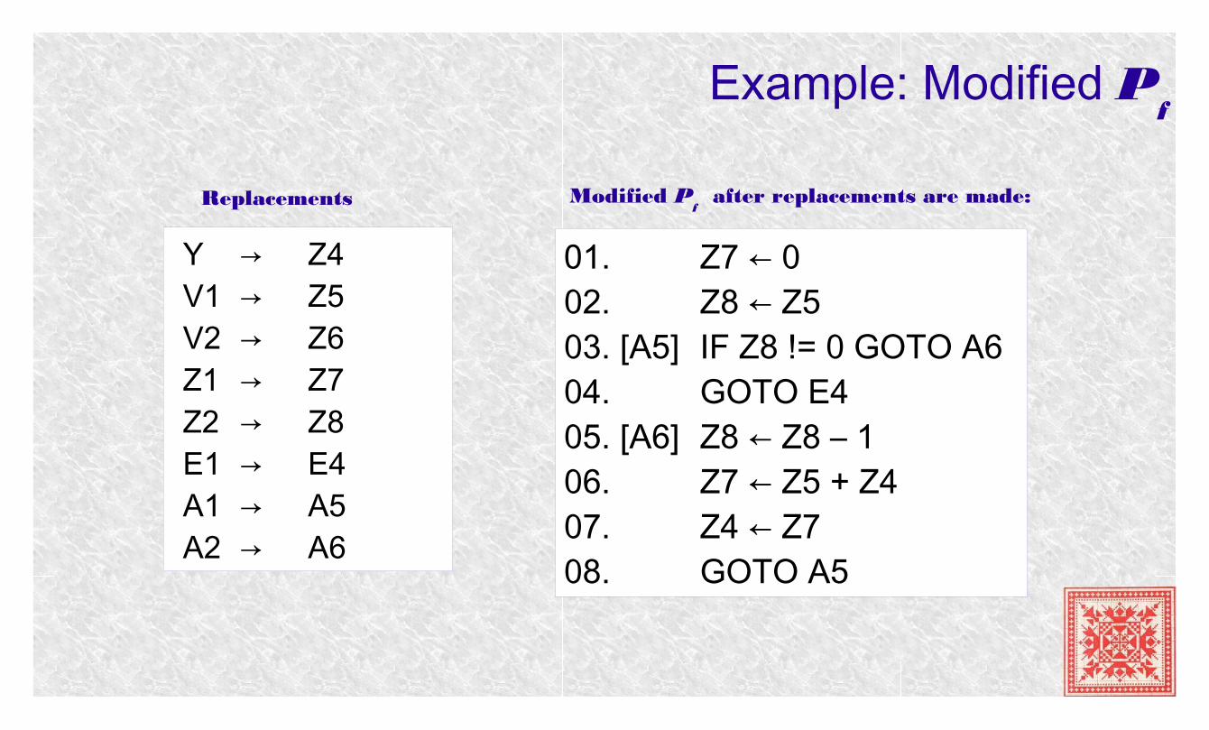
Example: Modified Pf
Replacements
01. Z7 ← 002. Z8 ← Z503. [A5] IF Z8 != 0 GOTO A604. GOTO E405. [A6] Z8 ← Z8 – 106. Z7 ← Z5 + Z407. Z4 ← Z708. GOTO A5
Modified Pf after replacements are made:
Y → Z4V1 → Z5 V2 → Z6 Z1 → Z7 Z2 → Z8 E1 → E4A1 → A5 A2 → A6
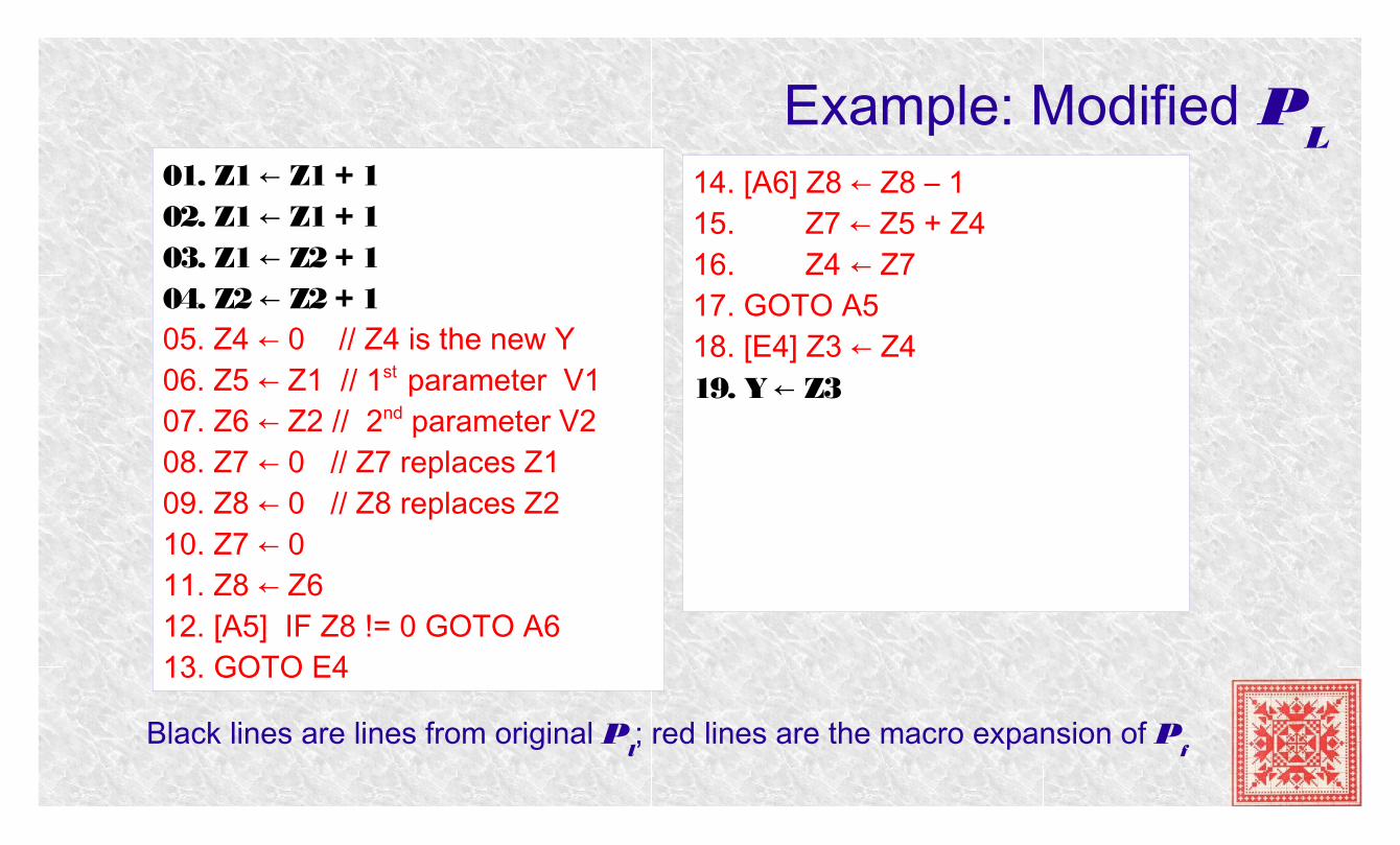
01. Z1 Z1 + 1←02. Z1 Z1 + 1←03. Z1 Z2 + 1←04. Z2 Z2 + 1←05. Z4 ← 0 // Z4 is the new Y06. Z5 ← Z1 // 1st parameter V107. Z6 ← Z2 // 2nd parameter V208. Z7 ← 0 // Z7 replaces Z109. Z8 ← 0 // Z8 replaces Z2 10. Z7 ← 011. Z8 ← Z612. [A5] IF Z8 != 0 GOTO A613. GOTO E4
Example: Modified PL
14. [A6] Z8 ← Z8 – 115. Z7 ← Z5 + Z416. Z4 ← Z717. GOTO A518. [E4] Z3 ← Z419. Y Z3 ←
Black lines are lines from original Pl; red lines are the macro expansion of P
f
Recursive Macro Expansion
• If the macro itself contains other macros, they can be recursively expanded in the same fashion
• When all the the expansions are done, the program contains only primitive instructions
• Since this expansion is algorithmic (the macros expands in the same way modulo variables and labels), we can assume that all macros contain only primitive instructions
The Point of Functional Macros
● The use of macros makes it easier for us to reason about computational properties of functions as mathematical objects
● If challenged by a mathematician on some function, we can write short, understandable programs to illustrate specific computational properties of that function
● If challenged by an computer scientist, we can expand the short programs into much longer programs written in the L primitive instructions
● Any computer scientist will readily acknowledge the realistic assumptions behind the primitive instructions of L
Reading Suggestions
● Ch. 2, Computability, Complexity, & Languages by Davis, Weyuker, Sigal
Recommended