The role of forcing and internal dynamics in explainingthe ‘‘Medieval Climate Anomaly’’
Hugues Goosse • Elisabeth Crespin • Svetlana Dubinkina •
Marie-France Loutre • Michael E. Mann • Hans Renssen •
Yoann Sallaz-Damaz • Drew Shindell
Received: 2 September 2011 / Accepted: 16 January 2012 / Published online: 4 February 2012
� Springer-Verlag 2012
Abstract Proxy reconstructions suggest that peak global
temperature during the past warm interval known as the
Medieval Climate Anomaly (MCA, roughly 950–1250 AD)
has been exceeded only during the most recent decades. To
better understand the origin of this warm period, we use
model simulations constrained by data assimilation estab-
lishing the spatial pattern of temperature changes that is
most consistent with forcing estimates, model physics and
the empirical information contained in paleoclimate proxy
records. These numerical experiments demonstrate that the
reconstructed spatial temperature pattern of the MCA can
be explained by a simple thermodynamical response of the
climate system to relatively weak changes in radiative
forcing combined with a modification of the atmospheric
circulation, displaying some similarities with the positive
phase of the so-called Arctic Oscillation, and with north-
ward shifts in the position of the Gulf Stream and Kuroshio
currents. The mechanisms underlying the MCA are thus
quite different from anthropogenic mechanisms responsible
for modern global warming.
Keywords Paleoclimate � Last millennium � Medieval
Climate Anomaly � Climate modelling � Data assimilation �Atmospheric and ocean dynamics � Radiative forcing
1 Introduction
Proxy temperature reconstructions indicate that the Medi-
eval Climate Anomaly (MCA, roughly 950–1250 AD) was
warm in many parts of the world (e.g., Hughes and Diaz
1994; Mann et al. 2008, 2009; Esper and Frank 2009;
Frank et al. 2010; Ljungqvist 2010; Graham et al. 2011).
Natural radiative forcing associated with quiescent volca-
nic activity and relatively high solar output may have
contributed to large-scale warmth (e.g. Crowley 2000). The
solar forcing may also have modified the large-scale
atmospheric circulation, inducing stronger mid-latitude
westerlies in winter and further warming in substantial
regions of the mid-latitude continents (e.g., Shindell et al.
2001, 2003). In addition, the internal variability of the
system, purely driven by its own dynamics, can also be
responsible for some of the reconstructed changes, in par-
ticular at regional scale (Goosse et al. 2005a; Servonnat
et al. 2010).
When driven by estimates of past natural and anthro-
pogenic forcings, models tend to produce warmer condi-
tions during the MCA than during the colder ‘‘Little Ice
Age’’ (LIA roughly 1400–1700 AD). The models, how-
ever, generally underestimate in magnitude the regional
changes observed in the reconstructions or fail to coincide
in timing with them (e.g., Gonzalez-Rouco et al. 2003;
H. Goosse (&) � E. Crespin � S. Dubinkina � M.-F. Loutre �Y. Sallaz-Damaz
Earth and Life Institute, Georges Lemaıtre Centre for Earth
and Climate Research, Universite Catholique de Louvain,
Chemin du Cyclotron, 2, 1348 Louvain-la-Neuve, Belgium
e-mail: [email protected]
M. E. Mann
Department of Meteorology and Earth and Environmental
Systems Institute, Pennsylvania State University,
University Park, PA, USA
H. Renssen
Section Climate Change and Landscape Dynamics,
Department of Earth Sciences, Vrije Universiteit Amsterdam,
Amsterdam, The Netherlands
D. Shindell
NASA Goddard Institute for Space Studies,
New York City, NY, USA
123
Clim Dyn (2012) 39:2847–2866
DOI 10.1007/s00382-012-1297-0
Goosse et al. 2005a; Ammann et al. 2007; Jungclaus et al.
2010; Servonnat et al. 2010; Swingedouw et al. 2011;
Gonzalez-Rouco et al. 2011). This disagreement could be
related to uncertainties in the forcing estimates or in the
dynamics of the models that would fail in reproducing the
adequate response to those forcings (e.g. Goosse et al.
2005b; Osborn et al. 2006). This could also be related to
the internal variability of the system as a model cannot
simulate the observed time evolution of the climate state if
it is not constrained directly by the observations, for
instance through data assimilation.
The goal of data assimilation is to combine information
coming from both simulations and observations, taking into
account their uncertainties, in order to have results com-
patible with all the elements (e.g. Talagrand 1997). Data
assimilation is relatively new in paleoclimatology (see
Widmann et al. 2010 for a recent review of the application
of data assimilation to the climate of the past millennium).
Our goal here is to apply this technique to provide addi-
tional insights into the processes that may underlie the
patterns of climate change during the MCA. To do so, we
perform simulations with the LOVECLIM climate model
(Goosse et al. 2010) using a so-called ‘‘particle filter’’ (van
Leeuwen 2009; Dubinkina et al. 2011) that constrains
model results to follow the signal provided by an annual
mean surface temperature reconstruction based on a global
proxy data network (Mann et al. 2009). Consequently, the
central variable in our discussion is also the annual mean
temperature, analyzing the simulated states obtained
through data assimilation to interpret the mechanism
responsible for the reconstructed changes. In particular, we
focus our attention on the extra-tropical Northern Hemi-
sphere, a data-rich region with a well-defined MCA sig-
nature. We thus acknowledge that, in this first study
devoted to the past millennium at this temporal and spatial
scale, we will investigate only one element of the MCA
since we will not discuss important characteristics such as
the seasonality of the changes, the connections between the
tropics and the extra-tropics and the variations in the
hydroclimate (e.g., Seager et al. 2007, Jones et al. 2009,
Burgman et al. 2010, Graham et al. 2011).
The paper is organized as follows. The methodology,
including the models used, the proxy based reconstruction,
the data assimilation technique and the experimental
design, is described in Sect. 2. The results are then pre-
sented in Sect. 3. Section 3.1 discusses the general char-
acteristics of the temperature changes in the LOVECLIM
model. The mechanisms responsible for those changes are
then analysed in Sect. 3.2. There, we also discuss in more
detail some of the hypotheses suggested up to now to
explain the MCA that were only briefly mentioned in the
introduction. In Sect. 3.3, a special focus is given to the
change in the heat balance of the Earth between the MCA
and the LIA. In order to consider the various processes that
may have played a role in the MCA–LIA transition,
including those not well reproduced in LOVECLIM, we
analyze complementary simulations performed with the
coupled atmosphere–ocean climate model GISS-ER in
Sect. 3.4. This allows a deeper analysis of the response of
the atmospheric circulation to the forcing. The role of the
forcing in the temperature changes between the MCA and
the LIA is then compared to the one observed during the
recent decades in Sect. 3.5. In addition to the information
provided on the MCA itself, this also demonstrates the
validity of our approach in a well studied period such as
the twentieth century characterized by large variations in
the forcing. Finally, conclusions are given in Sect. 4.
2 Description of the models, the proxy based
reconstruction, and the data assimilation method
2.1 Proxy-based reconstruction
In the data assimilation experiments, we make use of a
large-scale surface temperature reconstruction spanning the
past 1,500 years based on a global network of more than a
thousand proxy records (primarily tree ring, ice core, coral,
speleothem, and sediment records), as described in Mann
et al. (2009). Those records cover nearly all the globe but
with a higher density on northern hemisphere continents.
The reconstruction follow the RegEM climate field
reconstruction approach that has been tested thoroughly
using synthetic proxy networks derived from long-term
forced climate model simulations (Mann et al. 2007). As
the target of the reconstruction is annual mean temperature,
this methodology calibrates the proxy network against the
spatial information contained within the instrumental
annual mean surface temperature over an overlapping
(1850–1995) period. Uncertainties in the reconstructions
are then estimated from the residual unexplained variance
in statistical validation exercises (Mann et al. 2008, 2009).
This, for instance, shows that the skill of the reconstruction
is quite stable through time. As the reconstruction was
produced at the decadal timescale, a similar filtering is
applied to our simulations (see below) before performing
any analysis, using an 11-year Butterworth filter.
2.2 The climate model LOVECLIM
LOVECLIM 1.2 (Goosse et al. 2010) is a three-dimen-
sional Earth system model of intermediate complexity
whose components representing the atmosphere, the ocean,
the sea ice, and the land surface (including vegetation) are
activated here. The atmospheric component is ECBilt2
(Opsteegh et al. 1998), a quasi-geostrophic model with T21
2848 H. Goosse et al.: Medieval Climate Anomaly
123

horizontal resolution (corresponding to about 5.6� by 5.6�)
and 3 levels in the vertical. The ocean component is CLIO3
(Goosse and Fichefet 1999), which consists of an ocean
general circulation model coupled to a comprehensive
thermodynamic-dynamic sea-ice model. Its horizontal
resolution is of 3� by 3�, and there are 20 levels in the
ocean. ECBilt-CLIO is coupled to VECODE (Brovkin
et al. 2002), a vegetation model that simulates the
dynamics of two main terrestrial plant functional types,
trees and grasses, as well as desert. Its resolution is the
same as in ECBILT.
2.3 The particle filter
The particle filter (e.g., van Leeuwen 2009) used in the data
assimilation experiments is implemented as explained in
Dubinkina et al. (2011). First, an ensemble of 96 simula-
tions (called ‘particles’ or ensemble members) is initialized
for year 501 AD by adding to a single model state small
noise in the atmospheric streamfunction. Since the motion
in the atmosphere is chaotic, such a perturbation of the
atmospheric streamfunction guarantees a sufficiently wide
spread of the ensemble on a time scale of a few days at
most. Previous experiments (Goosse et al. 2006; Dubinkina
et al. 2011) have shown that 96 particles provide a good
sample of the large-scale variability of the system while
being affordable for simulations with data assimilation
covering several centuries. Each particle is then propagated
in time by the climate model. After 1 year, the likelihood
of each particle is computed from the difference between
the proxy-based reconstruction of annual mean tempera-
tures interpolated on the model grid and the simulated ones
on all available points northward of 30�N. This region is
selected as it is the focus of our study and because the skill
of the model is much higher in the extra-tropics than in the
tropical regions (Goosse et al. 2010). The particles are then
resampled according to their likelihood, i.e. to their ability
to reproduce the signal derived from the proxy records, as
in Liu and Chen (1998). The particles with low likelihood
are stopped, while the particles with a high likelihood are
copied a number of times proportional to their likelihood in
order to keep the total number of particles constant
throughout the period covered by the simulations, the new
weight of each particle being equal to one. A small noise is
again added in the atmospheric streamfunction of each
copy to obtain different time developments for the fol-
lowing year. The entire procedure is repeated sequentially
every year until the final year of calculation. Except for the
small perturbations applied at each resampling step, the
model dynamics is thus fully respected by the methodo-
logy, allowing us to analyze the physical process respon-
sible for the changes in a consistent way. The trajectory
selected by the filter could even, in theory, be obtained in a
single run without data assimilation covering the full per-
iod of interest. The probability of such an event is, how-
ever, virtually zero. In any case, it is in practice impossible
to launch a number of simulations without data assimila-
tion that is large enough to have a reasonable chance to find
one that is close to the reconstructed changes over the
whole past millennium, justifying the use of the particle
filter.
The likelihood is based on a Gaussian probability den-
sity (see van Leeuwen 2009; Dubinkina et al. 2011 for the
exact formulation). The error covariance matrix used to
compute this likelihood takes into account observation
errors and the error of representativeness (i.e., the error
related to the fact that data and models are not able to
represent the same spatial structures because of grid and
sub-grid scale variability present in the data and the lack of
observations in some regions to display a true mean on the
size of the model grid, see Kalnay 2003). We assume that
observation errors are uncorrelated in space and that the
error of representativeness is proportional to the covariance
between surface temperature at different locations in a long
control run of LOVECLIM (Sanso et al. 2008). The eval-
uation of the likelihood is performed on spatially smoothed
fields in which the features with scales smaller than
4,000 km are efficiently removed in order to emphasize the
contribution of large-scale structures. This smoothing is
taken into account in the estimate of the errors.
2.4 Experimental design of the simulations
with LOVECLIM
The simulations are performed over the period 501–2000
AD. They are driven by both natural forcings (orbital,
volcanic and solar) and anthropogenic forcings (changes in
greenhouse gas concentrations, in sulfate aerosols and
land-use) in the same way as in Goosse et al. (2010). The
total solar irradiance changes follow the reconstruction of
Muscheler et al. (2007), scaled to provide an increase of
1 W m-2 between the Maunder minimum (late seven-
teenth century) and the late twentieth century (i.e. a radi-
ative forcing of about 0.2 W m-2) and the long-term
changes in orbital parameters are derived from Berger
(1978). External forcing due to explosive volcanism
is prescribed according to Crowley et al. (2003). The
evolution of greenhouse gas concentrations is imposed
from a compilation of ice core records as explained in
Goosse et al. (2005a). The influence of anthropogenic
(AD 1850–2000) sulfate aerosols is represented through a
modification of surface albedo (Charlson et al. 1991). The
forcing due to anthropogenic land-use changes (affecting
surface albedo, surface evaporation and water storage) is
applied as in Goosse et al. (2005a), following Ramankutty
and Foley (1999). In order to take into account the
H. Goosse et al.: Medieval Climate Anomaly 2849
123

uncertainties in the forcing, a random component is added
to those natural and anthropogenic forcings for each
member of the simulations with data assimilation. This
random component, which is uncorrelated in time and
between the particles, follows a Gaussian probability dis-
tribution with a standard deviation of 0.4 W m-2. The
initial conditions in 501 AD are obtained from the results
of a transient simulation over the period 1–500 AD driven
by the same forcings starting from a quasi-equilibrium
simulation corresponding to the forcing estimates for year
1 AD.
We first perform an ensemble of 10 simulations without
data assimilation starting from those initial conditions in
501 AD. In the standard simulations with data assimilation
(referred to as STD when any confusion with another
experiment can occur), which starts from the same initial
conditions, the uncertainty of the reconstruction (Mann
et al. 2009) is assumed to be of 0.5�C. In addition to this
standard experiment, several sensitivity experiments have
been performed (Table 1) to illustrate the discussion pro-
posed in Sect. 3. In the first group of simulations, we
modify some parameters of the experimental design chosen
in STD. In Norandom, no additional forcing is applied,
while the one in Random0.8 is obtained from a distribution
with a standard deviation of 0.8 W m-2 instead of
0.4 W m-2 in STD. In Uncertain0.7, we assume an
uncertainty of the reconstruction of 0.7�C instead of 0.5�C
in STD. In the second group of experiments, we do not
simulate the full climate of the past millennium but only
constrain the model to follow the atmospheric circulation
anomalies obtained in STD during the MCA (CirculMCA)
and during the LIA (CirculMCA). In those experiments, no
forcing change is applied.
2.5 GISS-ER coupled atmosphere–ocean model
simulations
In addition to the simulation performed with LOVECLIM,
we analyze results from an ensemble of 6 climate simula-
tions using the coupled atmosphere–ocean climate model
GISS-ER without data assimilation, as in Mann et al.
(2009). This model has a more comprehensive represen-
tation of the atmospheric dynamical and physical processes
than LOVECLIM. Its results will thus be used in Sect. 3.4
to analyze in more detail the response of the atmospheric
circulation to the solar forcing.
Following a control run to establish stable initial con-
ditions, six transient runs extend from 850 to 1900 C.E.
Solar forcing is applied across the ultraviolet, visible and
infrared spectrum based on scaling the spectral variation
versus total irradiance as seen in modern satellite obser-
vations. The total irradiance through time is based on the
time series of Bard et al. (2007) derived from South Pole
ice core 10Be data and takes into account a small long-term
geomagnetic modulation (Korte and Constable 2005) and a
polar enhancement factor. The amplitude is scaled to give a
top-of-the-atmosphere incoming irradiance change of
2.2 Wm-2 between the Maunder Minimum and the late
twentieth century. This is twice the amplitude of previous
studies or models (Wang et al. 2005; Shindell et al. 2006),
and is chosen to provide a larger signal and test the
response to a more extreme forcing. It is equivalent to
Table 1 Description of the standard experiment and of the sensitivity experiments performed to illustrate the causes of temperature changes
during the MCA
Acronym Description Goal of the experiment
STD Standard experiment with data assimilation using natural and
anthropogenic forcings and an additional forcing selected from a
random distribution with a standard deviation of 0.4 W m-2
General analysis of the MCA–LIA transition
Norandom Experiment with data assimilation using natural and anthropogenic
forcings but without any additional forcing
Analysis of the role of the additional forcing
CirculMCA LOVECLIM is constrained using data assimilation to follow
the geopotential height simulated in the simulation with data
assimilation (STD) during the MCA (950–1250). A constant
pre-industrial forcing is applied in this experimentAnalysis of the influence of the circulation changes on
the temperature difference between the MCA and the
LIACirculLIA LOVECLIM is constrained using data assimilation to follow
the geopotential height simulated in the simulation with data
assimilation (STD) during the LIA (1400–1700). A constant
pre-industrial forcing is applied in this experiment
Random0.8 Experiment with data assimilation using natural and anthropogenic
forcings and an additional forcing selected from a random
distribution with a standard deviation of 0.8 W m-2 instead
of 0.4 W m-2
Analysis of the role of the additional forcing
Uncertain0.7 Experiment with data assimilation but assuming an uncertainty
of the proxy-based-reconstruction of 0.7�C instead of 0.5�C
Test of the sensitivity of the results to the estimation
of the uncertainty of the proxy-based-reconstruction
2850 H. Goosse et al.: Medieval Climate Anomaly
123
0.39 W m-2 radiative forcing between the Maunder Min-
imum and the late twentieth century, and about half that
between the MCA and LIA. The model includes the ozone
response to solar irradiance variations, which is parame-
terized from the results of prior GISS modeling using a full
atmospheric chemistry simulation (Shindell et al. 2006) for
computational efficiency. The ensemble mean results are
analyzed using time periods within (or very near) the MCA
and LIA periods selected in the reconstruction that maxi-
mized the solar forcing: 1125–1275 for the MCA,
1650–1750 for the LIA.
3 Results
3.1 Temperature simulated during the past millennium
LOVECLIM simulations without data assimilation yield
hemispheric-mean temperature histories similar to those
observed in other simulations employing a similar forcing
(Ammann et al. 2007; Jungclaus et al. 2010). The mean of
the ensemble of simulations also agrees well with proxy
surface temperature reconstructions (Mann et al. 2009) of
the past six centuries, but it fails to capture the warmer
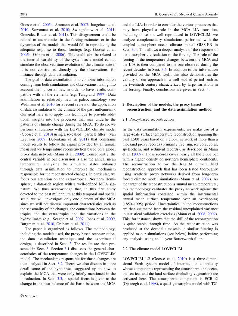
conditions of the earlier MCA interval (Fig. 1a). Never-
theless, the reconstruction generally lies in the range pro-
vided by the ensemble of simulations (not shown) that, in
addition to the forced response estimated through the
ensemble mean, also takes into account the internal vari-
ability simulated by the model.
The data assimilation strongly improves the agreement
over this earlier interval by constraining the model to
respond in a way that matches the reconstructed patterns of
temperature change. The improvement is also present
during the more recent past leading to a decadal correlation
between the mean simulation with assimilation and
instrumental record (Brohan et al. 2006) of r = 0.95
(p \ 0.01) over the 1850–2000 interval of overlap, com-
pared to a correlation of 0.84 for the ensemble mean of
simulations without data assimilation. This simulation with
Fig. 1 Temperature changes
between the MCA and the LIA.
a Anomaly of annual mean
temperature (�C) averaged over
the region 30�N–60�N in the
reconstruction of Mann et al.
(2009) (blue), in the mean of 10
simulations with LOVECLIM
without data assimilation (red)
and in simulation with data
assimilation (green). The
reference period is 1850–1980.
The time series have been
filtered using an 11-year
Butterworth filter to emphasize
decadal and longer timescales.
The uncertainty ranges
(2 standard deviations) are
shown for both the
reconstruction (violet) and
simulations with assimilation
(light green, the overlap between
the two uncertainty ranges is thus
in dark green; the range is not
shown for simulations without
assimilation). b Annual mean
surface temperature difference
between MCA (950–1250) and
LIA (1400–1700) in model
simulation with data
assimilation and c in the
reconstruction of Mann et al.
(2009). (Note: The color scale is
different in b, c because it has
been independently chosen to
highlight the large-scale
structure of the changes in
each case.)
H. Goosse et al.: Medieval Climate Anomaly 2851
123
data assimilation, however, does not quite reproduce the
level of warmth seen in the reconstruction over the interval
prior to AD 1100. This is perfectly compatible with the
data assimilation technique that assumes an error in the
reconstruction itself and thus has no reason to force
the model to give results identical to the one of the
reconstruction.
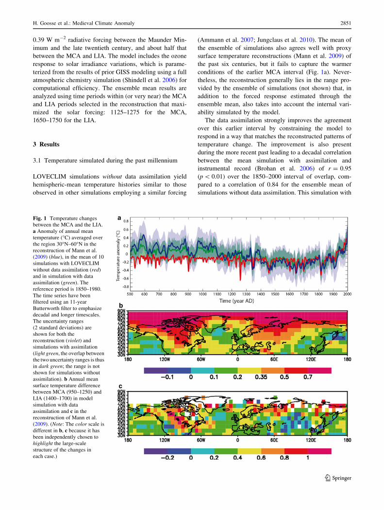
The effect of data assimilation can be illustrated by
analyzing the temperature distribution in the simulation
with data assimilation, in the simulation without data
assimilation and by comparing them with the reconstruc-
tion and its uncertainties (Fig. 2). For the first part of the
simulation (e.g., the years 1000–1010, Fig. 2a), the simu-
lation with data assimilation has its peak lying between the
one of the simulation without data assimilation and the
reconstruction. It is thus shifted towards higher tempera-
tures compared to the simulation without data assimilation
leading to a distribution displaying a larger overlap with
the range of the reconstruction. In a period when the
simulation without data assimilation has a mean close
to one of the reconstruction, as for the years 1650–1660
(Fig. 2b), the distribution of the simulation with data
assimilation has just a sharper peak than the one without
data assimilation, the mean being less affected. Data
assimilation helps thus to reduce the uncertainties on model
results for this period.
A useful way to measure the relative MCA warmth is
through the difference with the LIA. Frank et al. (2010), for
example, defines a MCA–LIA difference using the LIA
interval 1601–1630 and MCA interval 1071–1100, finding
a relative hemispheric-mean MCA warmth of 0.38�C,
which falls between the greater 0.44�C warmth based on
the Mann et al. (2009) reconstruction and the lesser warmth
of 0.33�C found in our simulation with data assimila-
tion for the same periods. Note, however, that taking a
slightly different interval for characterizing the LIA (i.e.
1620–1650) leads to a larger difference of 0.37�C in our
simulations with data assimilation.
More interesting, however, is the regional pattern of the
MCA–LIA surface temperature difference (Fig. 1b, c). In
both the reconstruction and the simulation with data
assimilation, notable warmth is evident in North Western
Russia and in the centre of the American continent, with
little relative warmth or even slight cooling over Eastern
Asia and parts of the North Atlantic southeast of
Greenland.
3.2 Causes of the temperature changes
in the simulation with data assimilation
We can now investigate the causes of the complex pattern
of MCA warmth. Firstly, the warmer conditions are partly
due to the natural and anthropogenic forcings applied in all
our simulations. It is illustrated by simulations without data
assimilation that display a response to this forcing char-
acterized by a general warming over the continents and
smaller changes over the oceans (Fig. 3a). This pattern
represents a classical response to a large-scale forcing (e.g.,
Hegerl et al. 2000) and can be explained by relatively
simple thermodynamic processes, the circulation changes
in LOVECLIM for the ensemble mean of the simulations
without data assimilation being very small.
Secondly, in addition to this radiative forcing, the par-
ticle filter can select among a random distribution the
forcing that leads to the best agreement with the recon-
struction. In our experiment with data assimilation,
this induces a slightly stronger forcing during the MCA
(?0.07 W m-2) and a weaker one during the LIA
(-0.06 W m-2) (Fig. 4). It is interesting to note that,
although the additional forcing imposed to each particle is
uncorrelated in time (see Sect. 2.4), the final forcing dis-
played in Fig. 4 has a clear time correlation which is
derived from the methodology itself and not from any
a priori assumption.
Fig. 2 Distribution of annual mean surface temperature anomaly
averaged over the area 30�N–60�N for a the period 1000–1010 and
b 1650–1660 in simulations without data assimilation (red) and with
data assimilation (green) compared to the reconstruction in blue,
including its error estimate (2 standard deviations)
2852 H. Goosse et al.: Medieval Climate Anomaly
123

We have evaluated the contribution of this additional
forcing in our standard experiment with data assimilation
(STD) by making the temperature difference between the
MCA and LIA in STD minus the one of a sensitivity
experiment with data assimilation in which no additional
random forcing is applied (Norandom, Table 1). It shows
that the additional forcing also contributes to a small
warming (Fig. 3b). This leads in the simulation with data
assimilation to a total effect of the forcing corresponding to
about 60% of the temperature change between the LIA and
the MCA averaged over the region 30�N–60�N.
Thirdly, the data assimilation also implies dynamic
changes in atmospheric circulation, associated with a
dipolar pattern of anomalous low (high) surface pressure
at high (low) latitudes in the MCA relative to the LIA
(Fig. 3e). These changes in geopotential height between
the two 300-year periods selected to represent the MCA
and the LIA are relatively modest, corresponding to 1–3%
Fig. 3 Causes of the temperature changes between the MCA
(950–1250) and the LIA (1400–1700). a Difference of annual mean
surface temperature (�C) between the MCA and LIA in an ensemble
of model simulations without data assimilation driven by the same
natural and anthropogenic forcings as the simulation with data
assimilation. b Temperature difference between the MCA and LIA in
the standard experiment with data assimilation (STD) minus the one
obtained in an experiment with data assimilation in which no
additional random forcing is applied (Norandom). c The difference in
annual mean surface temperature (in �C) between two sensitivity
experiments is shown: in the first one, LOVECLIM is constrained
using data assimilation to follow the geopotential height simulated in
the simulation with data assimilation during the MCA (CirculMCA);
in the second one, LOVECLIM is constrained to follow the
geopotential height simulated in the simulation with data assimilation
during the LIA (CirculLIA). d Sum of the fields displayed in a–
c. e Annual mean difference in geopotential height at 800 hPa (in m)
between MCA and LIA in model simulation with data assimilation
(STD)
H. Goosse et al.: Medieval Climate Anomaly 2853
123

of the climatological gradients in the model (Goosse et al.
2010). Nevertheless, as illustrated by comparing two
simulations, the first one being constrained using data
assimilation to follow the geopotential height simulated in
STD during the MCA (CirculMCA) while the second one
follows the geopotential height simulated in STD during
the LIA (CirculLIA), this atmospheric pattern induces
significant temperature changes (Fig. 3c). The temperature
increase is large at mid and high latitudes, in particular
over the Barents Sea, Northeast Europe and Canada, while
a cooling is simulated over the North Atlantic and in
Eastern Asia because of northerly winds there. The
mechanisms responsible for this temperature pattern are
relatively standard and have, for instance, been widely
studied in the framework of the NAO (e.g., Wallace et al.
1995; Hurrel 1995; Wanner et al. 2001). In addition to the
effect of the meridional wind component mentioned
above, the circulation changes are also associated with an
enhanced heat transport from ocean to land in many
regions. The ocean is thus generally cooling, and the land
is mostly warming. Because of the lower inertia of the
latter, the magnitude of the surface change is larger over
the continents resulting in mean temperature increase.
Nevertheless, because of the coarse resolution of our
model, the contrast between land and ocean is not clearly
expressed in coastal areas: some regions close to an ocean,
such as parts of the Western America and Western Europe,
are behaving more like the ocean itself than like conti-
nental areas.
We do not expect a perfect linear combination of the
different contributions. Nevertheless, when the effect of
this atmospheric pattern (Fig. 3c) is combined with the one
of the changes in the natural and anthropogenic forcings
(Fig. 3a) as well as with the one of the additional forcing
(Fig. 3b), the main characteristics of the reconstructed
change (Fig. 1c) and thus also of the simulation with data
assimilation (Fig. 1b) are well reproduced (Fig. 3d). This
shows that, on the basis of Fig. 3, we are able to explain the
major characteristics of the temperature changes in our
simulation with data assimilation.
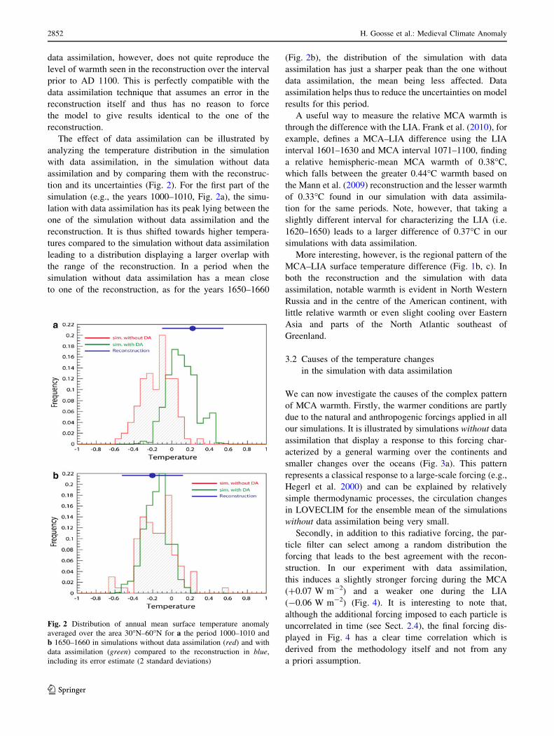
The annual mean changes in geopotential height mainly
reflect the winter signal (Fig. 5a), variations in summer
being much weaker. This winter pattern is not strictly
annular but has clear similarities with the positive phase of
the Arctic Oscillation (AO, also referred as the Northern
Annual Mode)/North Atlantic Oscillation (NAO) which
has been proposed to play a strong role in the observed
changes during the MCA (Shindell et al. 2001; Shindell
et al. 2003; Trouet et al. 2009; Mann et al. 2009). The
changes are not confined to the Atlantic sector and, in fact,
the dipole is stronger over the Pacific sector both in
LOVECLIM and in previous simulations with the climate
model GISS-ER (Mann et al. 2009). This characteristic is
also present in the AO (defined here as the first principal
component of the geopotential height at 800 hPa over the
region northward of 30�N) simulated by LOVECLIM
(Fig. 5b) and represents a bias compared to the observed
pattern seen in many models (e.g. Miller et al. 2006; see
also the GISS-ER results discussed in Sect. 3.4). When
analysing the probability distribution of the AO in the
model a clear shift towards its positive phase is seen during
the MCA compared to the LIA (Fig. 5c, d). The difference
in geopotential height displays some differences compared
to the AO itself, but this result demonstrates that a sig-
nificant part of the winter circulation changes in our sim-
ulations can be interpreted as a modification in the
distribution of the AO.
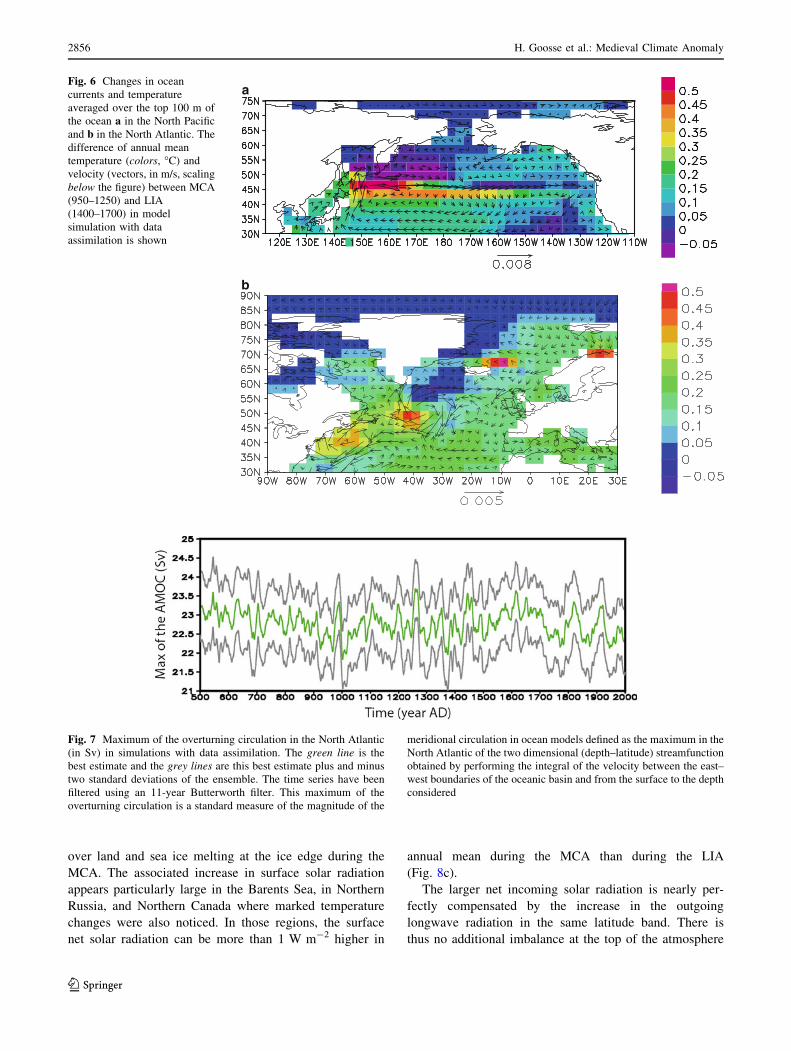
Associated with the modification of the atmospheric
circulation discussed above, significant changes in the
oceanic near-surface circulation are found between the
MCA and the LIA. A clear intensification and northward
shift of the subpolar gyre during the MCA are simulated in
the Pacific resulting in a large warming off the North coast
of Japan (Fig. 6a). A northward shift of the Gulf Stream
system is also simulated for the MCA in our standard
simulation with data assimilation resulting in a warming
off the east coast of North America between 35�N and
45�N (Fig. 6b). This is consistent with some past studies
that have argued for a potential role for such changes in the
position or intensity of the near-surface oceanic currents in
the West Atlantic and Pacific in long-term climate vari-
ability (Frankignoul et al. 2001; Lund et al. 2006; Kwon
et al. 2010; Swingedouw et al. 2011).
The intensification of the gyre in the Pacific is perfectly
compatible with the intensification of the winds there. This
is confirmed by the similar changes obtained by comparing
Fig. 4 Changes in the radiative forcing applied at the tropopause in
the simulation without data assimilation induced by natural and
anthropogenic forcings (red), in the standard simulation with data
assimilation (blue) and the difference between them (green). The
green curve represents thus the additional random forcing selected by
the particle filter in order to have the best agreement between the
model results and the proxy-based temperature reconstruction. The
time series have been filtered using an 11-year Butterworth filter
2854 H. Goosse et al.: Medieval Climate Anomaly
123
CirculMCA and the CirculLIA (not shown). Besides, the
changes in the North Atlantic appear to be more complex,
and their link with the wind forcing is less straightforward.
Nevertheless, as coarse resolution models such as
LOVECLIM have trouble to adequately represent the
subtle dynamics of western boundary currents (e.g., Kwon
et al. 2010), the mechanisms responsible for the changes in
currents in the North Atlantic will not be discussed in more
detail here.
The changes in oceanic meridional circulation appear to
play a smaller role in the transition between the MCA and
the LIA in our experiments with data assimilation. In
addition to clear decadal and multidecadal variations, the
maximum of the Meridional Overturning Circulation in the
North Atlantic displays only a modest reduction of 0.3 Sv
during the MCA relative to the LIA (Fig. 7). This decrease
is classical in models during the MCA (e.g. Swingedouw
et al. 2011) and, more generally, as a response to a
warming (Gregory et al. 2005). It induces a slightly
reduced northward heat transport in the Atlantic during the
MCA and thus a weak negative feedback on the tempera-
ture change, not a positive one that could explain the
simulated warming.
3.3 Changes in the heat balance between the MCA
and the LIA
Additional information on the mechanisms responsible for
the temperature changes between the MCA and the LIA
can be obtained by analysing the heat balance during
those two periods. The net incoming solar radiation at the
top of the atmosphere in tropical regions in the standard
simulation with data assimilation is about 0.3 W m-2
higher during the MCA than during the LIA (Fig. 8a).
This is close to the difference in total radiative forcing at
the tropopause between those two periods (0.28 W m-2,
see Fig. 4), illustrating the weak feedback on shortwave
flux in LOVECLIM in the tropics (Goosse et al. 2010).
The changes between the MCA and the LIA increase in
absolute value with latitude, reaching about 0.9 W m-2
close to the Pole. This characteristic appears even stron-
ger when analysing the relative changes of the net
incoming solar radiation as it varies from an increase of
0.1% at the Equator to 0.25% at 50�N and more than 1%
at high latitudes (Fig. 8b). This amplification of the
response at high latitudes is mainly due to lower surface
albedo values caused by the reduction of the snow cover
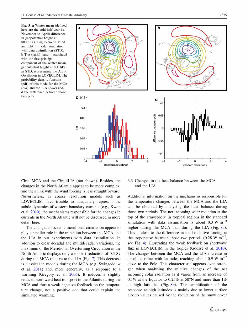
Fig. 5 a Winter mean (defined
here are the cold half year i.e.
November to April) difference
in geopotential height at
800 hPa (in m) between MCA
and LIA in model simulation
with data assimilation (STD).
b The spatial pattern associated
with the first principal
component of the winter mean
geopotential height at 800 hPa
in STD, representing the Arctic
Oscillation in LOVECLIM. The
probability density function
(pdf) of this mode for the MCA
(red) and the LIA (blue) and,
d the difference between those
two pdfs
H. Goosse et al.: Medieval Climate Anomaly 2855
123
over land and sea ice melting at the ice edge during the
MCA. The associated increase in surface solar radiation
appears particularly large in the Barents Sea, in Northern
Russia, and Northern Canada where marked temperature
changes were also noticed. In those regions, the surface
net solar radiation can be more than 1 W m-2 higher in
annual mean during the MCA than during the LIA
(Fig. 8c).
The larger net incoming solar radiation is nearly per-
fectly compensated by the increase in the outgoing
longwave radiation in the same latitude band. There is
thus no additional imbalance at the top of the atmosphere
a
b
Fig. 6 Changes in ocean
currents and temperature
averaged over the top 100 m of
the ocean a in the North Pacific
and b in the North Atlantic. The
difference of annual mean
temperature (colors, �C) and
velocity (vectors, in m/s, scaling
below the figure) between MCA
(950–1250) and LIA
(1400–1700) in model
simulation with data
assimilation is shown
Fig. 7 Maximum of the overturning circulation in the North Atlantic
(in Sv) in simulations with data assimilation. The green line is the
best estimate and the grey lines are this best estimate plus and minus
two standard deviations of the ensemble. The time series have been
filtered using an 11-year Butterworth filter. This maximum of the
overturning circulation is a standard measure of the magnitude of the
meridional circulation in ocean models defined as the maximum in the
North Atlantic of the two dimensional (depth–latitude) streamfunction
obtained by performing the integral of the velocity between the east–
west boundaries of the oceanic basin and from the surface to the depth
considered
2856 H. Goosse et al.: Medieval Climate Anomaly
123

that would require changes in the meridional heat trans-
port. In a consistent way, oceanic and atmospheric
meridional heat transports remain more or less similar
between the LIA and the MCA in our experiments (not
shown). The role of the changes in oceanic and atmo-
spheric circulations have thus either a regional effect, as
discussed above for the currents close to the western
boundaries of the oceans, or have an influence on the
zonal atmospheric transport, in particular because of
enhanced exchanges between the land and the oceanic
domains. We should, however, remind that our model has
a coarse resolution in the atmosphere and is thus not able
to account well for potential changes in the transport by
transient eddies that play a dominant role in the meridi-
onal heat exchanges at mid latitudes. The situation is even
worse in the ocean where the effect of those eddies is
parameterized in a relatively simple way (Goosse et al.
2010). It would thus be useful to check if our conclusions
remain valid in high resolution models representing more
accurately those processes.
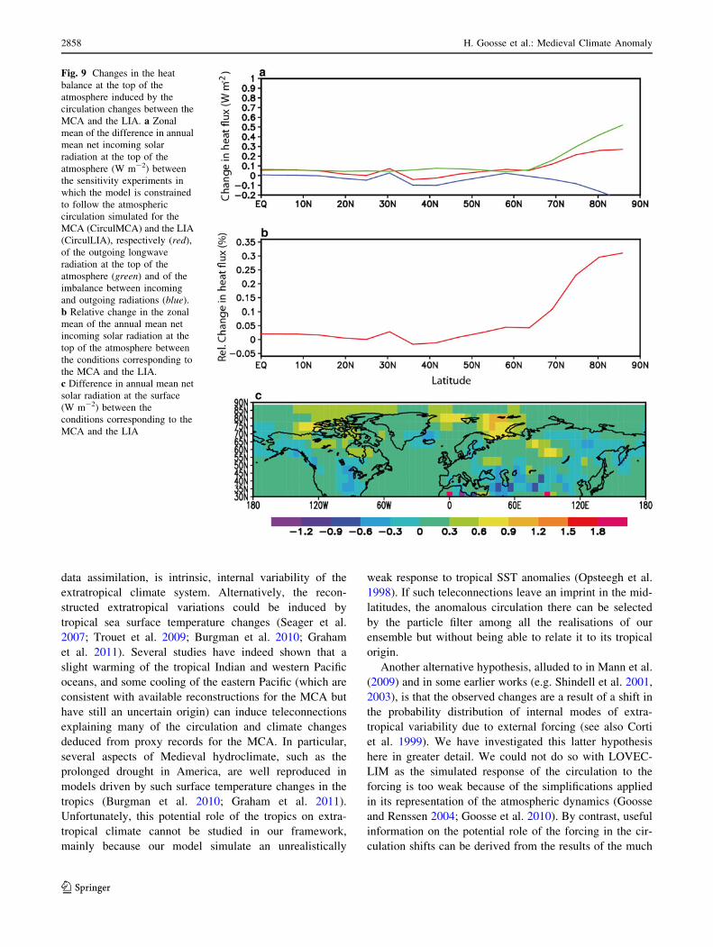
Besides, the circulation changes still have an indirect
impact on the heat balance. As they induce a warming in
many continental areas and in the Arctic, they contribute
to the changes in surface albedo. This is illustrated in
CirculMCA and CirculLIA. Although no modification of
the radiative forcing is applied in those experiments, the
surface solar radiation is higher in the warmer regions and
lower in the colder regions in response to the circulation
changes, resulting in a net increase in the net incoming
solar radiations at mid and high latitudes (Fig. 9).
3.4 Forced response in the GISS coupled
atmosphere–ocean model ER simulations
One hypothesis to explain the small but persistent circu-
lation shifts in STD, put forward by our simulation with
Fig. 8 Changes in the heat
balance at the top of the
atmosphere between the MCA
and the LIA. a Zonal mean of
the difference in annual mean
net incoming solar radiation at
the top of the atmosphere
(W m-2) between the MCA
(950–1250) and the LIA
(1400–1700) in the standard
model simulation with data
assimilation (red), of the
outgoing longwave radiation at
the top of the atmosphere
(green) and of the imbalance
between incoming and outgoing
radiations (blue). b Relative
change in the zonal mean of the
annual mean net incoming solar
radiation at the top of the
atmosphere between the MCA
and the LIA. c Difference in
annual mean net solar radiation
at the surface (W m-2) between
the MCA and the LIA
H. Goosse et al.: Medieval Climate Anomaly 2857
123
data assimilation, is intrinsic, internal variability of the
extratropical climate system. Alternatively, the recon-
structed extratropical variations could be induced by
tropical sea surface temperature changes (Seager et al.
2007; Trouet et al. 2009; Burgman et al. 2010; Graham
et al. 2011). Several studies have indeed shown that a
slight warming of the tropical Indian and western Pacific
oceans, and some cooling of the eastern Pacific (which are
consistent with available reconstructions for the MCA but
have still an uncertain origin) can induce teleconnections
explaining many of the circulation and climate changes
deduced from proxy records for the MCA. In particular,
several aspects of Medieval hydroclimate, such as the
prolonged drought in America, are well reproduced in
models driven by such surface temperature changes in the
tropics (Burgman et al. 2010; Graham et al. 2011).
Unfortunately, this potential role of the tropics on extra-
tropical climate cannot be studied in our framework,
mainly because our model simulate an unrealistically
weak response to tropical SST anomalies (Opsteegh et al.
1998). If such teleconnections leave an imprint in the mid-
latitudes, the anomalous circulation there can be selected
by the particle filter among all the realisations of our
ensemble but without being able to relate it to its tropical
origin.
Another alternative hypothesis, alluded to in Mann et al.
(2009) and in some earlier works (e.g. Shindell et al. 2001,
2003), is that the observed changes are a result of a shift in
the probability distribution of internal modes of extra-
tropical variability due to external forcing (see also Corti
et al. 1999). We have investigated this latter hypothesis
here in greater detail. We could not do so with LOVEC-
LIM as the simulated response of the circulation to the
forcing is too weak because of the simplifications applied
in its representation of the atmospheric dynamics (Goosse
and Renssen 2004; Goosse et al. 2010). By contrast, useful
information on the potential role of the forcing in the cir-
culation shifts can be derived from the results of the much
Fig. 9 Changes in the heat
balance at the top of the
atmosphere induced by the
circulation changes between the
MCA and the LIA. a Zonal
mean of the difference in annual
mean net incoming solar
radiation at the top of the
atmosphere (W m-2) between
the sensitivity experiments in
which the model is constrained
to follow the atmospheric
circulation simulated for the
MCA (CirculMCA) and the LIA
(CirculLIA), respectively (red),
of the outgoing longwave
radiation at the top of the
atmosphere (green) and of the
imbalance between incoming
and outgoing radiations (blue).
b Relative change in the zonal
mean of the annual mean net
incoming solar radiation at the
top of the atmosphere between
the conditions corresponding to
the MCA and the LIA.
c Difference in annual mean net
solar radiation at the surface
(W m-2) between the
conditions corresponding to the
MCA and the LIA
2858 H. Goosse et al.: Medieval Climate Anomaly
123

Fig. 10 Principal component analysis of the cold half year (Novem-
ber to April) sea level pressure in GISS-ER simulations over the past
millennium. a The spatial pattern of the second eigenvector (asso-
ciated with the time series of Principal Component PC2) and b of
forth eigenvector (associated with PC4). c, d, the difference (in black)
in the distribution of PC2 and PC4 between two periods of the MCA
and LIA characterized by a strong difference in solar irradiance
(in units of standard deviations). The full distribution is given on
e, f in red for the MCA and in blue for the LIA. The significance of
the difference is evaluated by comparing it with one (in blue) and two
(in red) standard deviations of this distribution using the same number
of samples from a control run
H. Goosse et al.: Medieval Climate Anomaly 2859
123

more sophisticated GISS-ER coupled atmosphere–ocean
climate model by comparing its results during sub-periods
of high and low solar irradiance during the MCA and LIA,
respectively.
In the GISS-ER model, the solar forcing clearly shifts
the probability distribution of the key extratropical atmo-
spheric circulation modes as shown by an analysis of the
leading principal components of sea level pressure (PCs,
also commonly referred to as empirical orthogonal func-
tions, or EOFs). The spatial pattern associated with the 2nd
ranked principal component (‘‘PC2’’) displays a zonally-
symmetric structure similar to the AO (Fig. 10a) but with a
stronger centre of action in the Pacific. Its distribution is
moved towards the positive phase (Fig. 10 c, e), while the
more zonally-asymmetric 4th ranked PC (‘‘PC4’’)
(Fig. 10b) shifts towards the negative phase (Fig. 10d, f).
The distribution of the other PCs, which could not be
associated simply to any standard mode of atmospheric
variability, is less influenced by the solar forcing.
Principal components 2 and 4 explain 21 and 8% of the
variance, respectively. Furthermore, the shifts in their
probability distribution are modest in comparison with the
intrinsic internal variability. They are nonetheless respon-
sible for a multi-decadal high surface pressure anomaly
over the North Atlantic and North/Central Pacific and for a
negative surface pressure anomaly at higher latitudes of
about 60�N–70�N. The associated circulation changes lead
to significant temperature variations, as shown in Mann
et al. (2009, see their Fig. 4). This clearly illustrates the
potential role of such probability shifts induced by solar
activity in the MCA–LIA transition.
3.5 Role of the forcing in the MCA–LIA transition
compared to the twentieth century warming
In the standard simulation with data assimilation (STD), we
assume that the uncertainty in the forcing can be repre-
sented by an additional forcing derived from a Gaussian
distribution with a standard deviation of 0.4 W m-2. This
may appear large compared to recent estimates (Schmidt
et al. 2011), but such a high value can also be a way to
represent the uncertainty in model response. For instance,
if the model tends to underestimate the response to a
forcing, the particle filter will likely select a particle with a
stronger forcing in order to have a closer match between
simulated and reconstructed temperature changes. Fur-
thermore, there are still uncertainties in the exact magni-
tude of past changes in radiative forcing, in particular the
Fig. 11 Temperature changes
in sensitivity experiments.
a Anomaly of annual mean
temperature (�C) averaged over
the region 30�N–60�N in the
standard simulation with data
assimilation (green) and in two
sensitivity experiments in which
no additional random forcing is
applied (experiment Norandom,
dark blue) and in which the
standard deviation of the
uncertainty of the forcing is
assumed to be 0.8 W m-2
(experiment Random0.8, lightblue). The reconstruction of
Mann et al. (2009) is in red. The
reference period is 1850–1980.
As in Fig. 1, the time series
have been filtered using an
11-year Butterworth filter. The
grey lines represent the range of
the standard simulation with
data assimilation (best estimate
plus and minus two standard
deviations). b Annual mean
surface temperature difference
between MCA (950–1250) and
LIA (1400–1700) in Norandom.
c The same as b but in
Random0.8
2860 H. Goosse et al.: Medieval Climate Anomaly
123

changes in solar irradiance that can justify such a high
value (e.g. Schmidt et al. 2011; Shapiro et al. 2011).
In order to further analyze the role of such an additional
forcing and to further highlight the way the data assimi-
lation method works, we have compared the results of STD
with the ones of two additional sensitivity experiments. In
Norandom, already discussed above, no additional forcing
is applied. In the second sensitivity experiment, we assume
for the distribution of the additional forcing a very high
standard deviation of 0.8 W m-2, to study the behaviour of
the system in an extreme case (Random0.8).
As expected, because of the larger standard deviation of
the forcing, the simulated temperature during the MCA
increases in Random0.8, while it decreases in Norandom
compared to the STD. Nevertheless, the differences appear
relatively small. For the LIA, the difference in annual mean
temperature averaged over the region 30�N–60�N is
smaller than 0.03�C between the three simulations
(Fig. 11a). For the MCA, the range of the three simulations
is 0.09�C. Slightly larger differences appear for some
periods, such as around 1000 AD, but even in that case the
three experiments are relatively close to each other. The
spatial temperature pattern is also similar in the three
experiments, only with a higher large-scale warming in
Random0.8 compared to STD and then in STD compared
to Norandom (Fig. 11b, c). Furthermore, the changes in
atmospheric circulation in all the experiments have the
same characteristics (Fig. 12). This demonstrates that this
pattern, which strongly contributes to the spatial structure
of the warming during the MCA, is very robust in our
experiments. This pattern also depends weakly on reason-
able changes of the uncertainty assigned to the recon-
struction (see ‘‘Appendix’’).
The larger warming is achieved in Random0.8 thanks to
a positive additional forcing of 0.2 W m-2 during the
MCA and a negative one during the LIA of 0.14 W m-2
(Fig. 13). As expected, it appears thus also possible to
explain the MCA–LIA transition using a larger forcing
difference between those two periods than in Norandom
and STD. Those values of the forcing, however, are quite
high and incompatible with present best estimates because
of the extreme hypothesis followed in Random0.8. Fur-
thermore, the simulated changes in Random0.8 are not
strongly different from the ones obtained in Norandom and
STD, and both experiments are compatible with the proxy
based reconstruction within its own error bars. Conse-
quently, there is no need to invoke a strong radiative
forcing between the MCA and LIA to explain the recon-
structed temperature changes. From the present estimates
Fig. 12 Annual mean difference in geopotential height at 800 hPa (in
m) between MCA (950–1250) and LIA (1400–1700) in additional
model simulations with data assimilation. Compared to the standard
experiment in a, no additional random forcing is applied (experiment
Norandom) and in b the standard deviation of the uncertainty of the
forcing is assumed to be 0.8 W m-2 (experiment Random0.8)
Fig. 13 Additional random forcing selected by the particle filter in
the standard experiment with data assimilation (STD, in green) and in
a sensitivity experiment in which the standard deviation of the
uncertainty of the forcing is assumed to be 0.8 W m-2 (experiment
Random0.8, in blue)
H. Goosse et al.: Medieval Climate Anomaly 2861
123
of past forcing, we can rather conclude that the role of the
forcing is very likely overestimated in Random0.8.
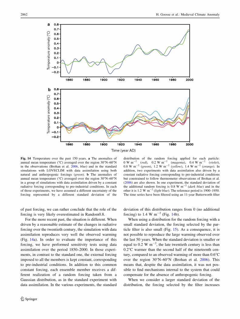
For the more recent past, the situation is different. When
driven by a reasonable estimate of the changes in radiative
forcing over the twentieth century, the simulation with data
assimilation reproduces very well the observed warming
(Fig. 14a). In order to evaluate the importance of this
forcing, we have performed sensitivity tests using data
assimilation over the period 1850–2000. In those experi-
ments, in contrast to the standard one, the external forcing
imposed to all the members is kept constant, corresponding
to pre-industrial conditions. In addition to this common
constant forcing, each ensemble member receives a dif-
ferent realization of a random forcing taken from a
Gaussian distribution, as in the standard experiment with
data assimilation. In the various experiments, the standard
deviation of this distribution ranges from 0 (no additional
forcing) to 1.4 W m-2 (Fig. 14b).
When using a distribution for the random forcing with a
small standard deviation, the forcing selected by the par-
ticle filter is also small (Fig. 15). As a consequence, it is
not possible to reproduce the large warming observed over
the last 50 years. When the standard deviation is smaller or
equal to 0.2 W m-2, the late twentieth century is less than
0.2�C warmer than the second half of the nineteenth cen-
tury, compared to an observed warming of more than 0.6�C
over the region 30�N–60�N (Brohan et al. 2006). This
means that, despite the data assimilation, it was not pos-
sible to find mechanisms internal to the system that could
compensate for the absence of anthropogenic forcing.
When we consider a larger standard deviation of the
distribution, the forcing selected by the filter increases
Fig. 14 Temperature over the past 150 years. a The anomalies of
annual mean temperature (�C) averaged over the region 30�N–60�N
in the observations (Brohan et al. 2006, blue) and in the standard
simulations with LOVECLIM with data assimilation using both
natural and anthropogenic forcings (green). b The anomalies of
annual mean temperature (�C) averaged over the region 30�N–60�N
in a group of simulations with data assimilation driven by a constant
radiative forcing corresponding to pre-industrial conditions. In each
of those experiments, we have assumed a different uncertainty of the
forcing represented by a different standard deviation of the
distribution of the random forcing applied for each particle:
0 W m-2 (red), 0.2 W m-2 (magenta), 0.4 W m-2 (violet),0.8 W m-2 (green), 1.2 W m-2 (yellow), 1.4 W m-2 (orange). In
addition, two experiments with data assimilation also driven by a
constant radiative forcing corresponding to pre-industrial conditions
but constrained to follow thermometer observations of Brohan et al.
(2006) are also shown. In one experiment, the standard deviation of
the additional random forcing is 0.8 W m-2 (dark blue) and in the
other it is 1.2 W m-2 (light blue). The reference period is 1900–1950.
The time series have been filtered using an 11-year Butterworth filter
2862 H. Goosse et al.: Medieval Climate Anomaly
123

strongly. For the largest value, we reach at the end of the
twentieth century a forcing of more than 1 W m-2, which
is a bit lower than the best estimate of 1.6 W m-2 (Forster
et al. 2007) but well in the range of uncertainty of this
forcing. As a result, the temperature increases strongly
during the twentieth century, in particular during the last
decades, but the temperature is still lower than the
observed one. We must keep in mind that in those exper-
iments, we start from a highly biased estimate of the
forcing, considering that the best prior estimate is a con-
stant forcing and that positive and negative values over the
twentieth century are as likely. This could partly explain
the bias to low temperature in all those sensitivity experi-
ments. The choice of the dataset selected for the data
assimilation also has an impact. If we perform simulations
with data assimilation constrained to follow the HADC-
RUT3 dataset (Brohan et al. 2006) as in Dubinkina et al.
(2011), the bias becomes very small when the forcing is
derived from a distribution using a large standard deviation
(Fig. 14b). Finally, the range of those simulations with
different estimates of the uncertainty of the radiative
forcing is of 0.39�C, i.e. at least 4 times more than in our
experiments for the LIA and the MCA, even if we take into
account the extreme case of experiment Random0.8.
We should insist that the goal of those sensitivity
experiments was not to obtain an optimal reconstruction of
the temperature or of the forcing over the twentieth century.
In that case, it would be better to start from reasonable
estimates of the forcing and of its uncertainty as in the
standard experiment. We neither wanted to discuss specif-
ically the dynamics of the recent temperature changes that
have already been widely studied but rather to demonstrate
the validity of our approach for a period when the role of the
forcing is dominant. In our comparison between the twen-
tieth century warming and the MCA–LIA transition, we
must also acknowledge that data availability is much lower
and the uncertainty of data is higher for the earlier periods.
This has an impact on our estimation of the role of the
forcing as more reliable estimates of the spatial temperature
change or of the forcing would provide stronger constrains
on our results and thus more precise conclusions.
4 Conclusions
We can conclude that it is possible to explain the recon-
structed temperature changes during the MCA by a simple
thermodynamic response to relatively weak changes in the
forcing (of the order of 0.25 W m-2 between the MCA and
the LIA in our simulation with data assimilation), com-
bined with the influence of oceanic and atmospheric cir-
culation changes. The first contributor, which sets up a
general warming, can be captured simply by energy bal-
ance considerations. The latter one amplifies the warming
and imposes its spatial structure. It is characterized in our
experiments with data assimilation by stronger westerlies
over mid latitudes, sharing thus some clear similarities with
the positive phase of the AO, as well as by a northward
shift and an intensification of the western boundary current
in the Pacific and, to a smaller extent, in the Atlantic.
Those circulation changes in LOVECLIM are mainly
related to internal dynamics. The timing of the recon-
structed changes can thus be reproduced by the model only
if its development is directly constrained through data
assimilation. The complementary results of the GISS-ER
model suggest alternatively that the circulation shifts can
be partly a consequence of the dynamical response to the
radiative forcing. LOVECLIM, because of its simplified
dynamics, would underestimate this forced contribution,
compensating this bias by a stronger shift of the internal
variability. Nevertheless, GISS-ER results were included
here to discuss only qualitatively the potential mechanisms.
Current uncertainties in the forcing and in the relevant
physical processes preclude any definitive quantitative
conclusions regarding the magnitude of this compensation
in LOVECLIM, and thus it is still challenging to determine
precisely the true role of internal versus external cause in
the circulation changes.
Our results are based on the hypothesis chosen, in par-
ticular on our a priori estimate of the forcing and of its
uncertainty. In our standard experiment, following the
present-day knowledge, we have selected a relatively weak
solar forcing and an uncertainty which may already appear
large compared to some analyses. Nevertheless, experiments
with an even larger uncertainty confirm that, as expected, the
warm conditions during the MCA could also be explained as
Fig. 15 Additional random forcing selected by the particle filter in
experiments driven by a constant radiative forcing corresponding to
pre-industrial conditions. In each of those experiments, we have
assumed a different uncertainty of the forcing represented by a
different standard deviation of the distribution of the random forcing
applied for each particle: 0.2 W m-2 (magenta), 0.4 W m-2 (violet),0.8 W m-2 (green), 1.2 W m-2 (yellow), 1.4 W m-2 (orange). An
11-year running mean has been applied to the time series
H. Goosse et al.: Medieval Climate Anomaly 2863
123

a response to a larger forcing change. This larger forcing
does not presently provide the most likely hypothesis but
may be kept in mind if new evaluations of the range of
possible forcing variations are proposed in the future. But,
even with this forcing, the circulation changes simulated in
our simulation with data assimilation appear very robust.
Anyway, the transition between the MCA and the LIA,
in which only a weak forcing is necessary to have results
compatible with the reconstruction, contrasts with the
recent decades for which a direct response to a much
stronger radiative forcing is required to provide a satis-
factory explanation for the observed large-scale warming
(e.g. Hegerl et al. 2007). In our experiments, a forcing of
the order of 1 W m-2 is needed to reproduce the recent
warming, even with data assimilation. This indicates that
our methodology was able to catch the different contribu-
tions of the forcing in these periods.
Acknowledgments We thank E. Zorita and R. Wilson for com-
ments and all the scientists that collected and analysed the proxy data
used in this work. H.G. is Senior Research Associate with the Fonds
National de la Recherche Scientifique (FRS-FNRS-Belgium). This
work is supported by the FRS-FNRS and by the Belgian Federal
Science Policy Office (Research Program on Science for a Sustainable
Development) and by EU (project Past4future). M.E.M.
acknowledges support from the NSF Paleoclimate program (grant
number ATM-0902133). Aurelien Mairesse helped in the design of
Fig. 1. Computational resources have been provided by the super-
computing facilities of the Universite Catholique de Louvain (CISM/
UCL) and the Consortium des Equipements de Calcul Intensif en
Federation Wallonie Bruxelles (CECI) funded by the Fond de la
Recherche Scientifique de Belgique (FRS-FNRS).
Appendix: Sensitivity to the uncertainty
of the reconstruction
The data assimilation methodology applied here provides
estimates of the uncertainties. In addition, to test the validity
of our conclusions, we have launched one supplementary
simulation with data assimilation (Fig. 16) in which we use
a slightly higher value for the uncertainty associated with
the proxy-based reconstruction (0.7�C instead of 0.5�C)
(Experiment Uncertain0.7). For the mean temperature over
the region 30�N–60�N, the results of this new experiment
are remarkably similar to the one of the standard simulation.
The obtained spatial patterns of the temperature as well as
the changes in atmospheric circulation (Fig. 17) are also in
very close agreement to the ones described for the standard
experiment. Locally, some small differences can be noticed,
Fig. 16 Temperature changes in an additional model simulation with
data assimilation in which, compared to the standard experiment, the
uncertainty of the proxy-based reconstruction is assumed to be 0.7�C
instead of 0.5�C (experiment Uncertain0.7). a Anomaly of annual
mean temperature (�C) averaged over the region 30�N–60�N in the
standard simulation with data assimilation (green) and in Uncertain0.7
(light blue). The reference period is 1850–1980. As in Fig. 1, the time
series have been filtered using an 11-year Butterworth filter. The greylines represent the range of the standard simulation with data
assimilation (best estimate plus and minus two standard deviations).
b Annual mean surface temperature difference between MCA
(950–1250) and LIA (1400–1700) in the experiment Uncertain0.7
2864 H. Goosse et al.: Medieval Climate Anomaly
123

but they are too small to challenge the interpretation
deduced from the results of the standard simulation, illus-
trating that our results are robust at least when using the
model and proxy based reconstruction applied here.
References
Ammann CM, Joos F, Schimel DS, Otto-Bliesner BL, Tomas RA
(2007) Solar influence on climate during the past millennium:
results from transient simulations with the NCAR climate system
model. Proc Natl Acad Sci USA 104:3713–3718
Bard E, Raisbeck G, Yiou F, Jouzel J (2007) Comment on ‘‘Solar
activity during the last 1000 yr inferred from radionuclide
records’’ by Muscheler et al. (2007). Quat Sci Rev 26:2301–2308
Berger AL (1978) Long-term variations of daily insolation and
quaternary climatic changes. J Atmos Sci 35:2363–2367
Brohan P, Kennedy JJ, Harris I, Tett SFB, Jones PD (2006) Uncertainty
estimates in regional and global observed temperature changes: a
new data set from 1850. J Geophys Res 111:Art. No. D12106
Brovkin V, Bendtsen J, Claussen M, Ganopolski A, Kubatzki C,
Petoukhov V, Andreev A (2002) Carbon cycle, vegetation and
climate dynamics in the Holocene: experiments with the
CLIMBER-2 model. Global Biogeochem Cycles 16. doi:
10.1029/2001GB001662
Burgman R, Seager R, Clement A, Herweijer C (2010) Role of
tropical Pacific SSTs in global Medieval hydroclimate: a
modeling study. Geophys Res Lett 37:L06705. doi:10.1029/2009
GL042239
Charlson RJ, Langner J, Rodhe H, Leovy CB, Warren SG (1991)
Perturbation of the northern hemisphere radiative balance by
backscattering from anthropogenic sulfate aerosols. Tellus 43
AB:152–163
Corti S, Molteni F, Palmer TN (1999) Signature of recent climate
change in frequencies of natural atmospheric circulation
regimes. Nature 398:799–802
Crowley TJ (2000) Causes of climate change over the past
1000 years. Science 289:270–277
Crowley TJ, Baum SK, Kim KY, Hegerl GC, Hyde WT (2003)
Modeling ocean heat content changes during the last millennium.
Geophys Res Lett 30:1932
Dubinkina S, Goosse H, Sallaz-Damaz Y, Crespin E, Crucifix M
(2011) Testing a particle filter to reconstruct climate changes
over the past centuries. Int J Bifurc Chaos (in press)
Esper J, Frank D (2009) The IPCC on a heterogeneous Medieval
warm period. Clim Change 94:267–273
Forster P, Ramaswamy V, Artaxo P, Berntsen T, Betts R, Fahey DW,
Haywood J, Lean J, Lowe DC, Myhre G, Nganga J, Prinn R,
Raga G, Schulz M, Van Dorland R (2007) Changes in
atmospheric constituents and in radiative forcing. In: Solomon
S, Qin D, Manning M, Chen Z, Marquis M, Averyt KB, Tignor
M, Miller HL (eds) Climate change 2007: the physical science
basis. Contribution of Working Group I to the fourth assessment
report of the Intergovernmental Panel on Climate Change.
Cambridge University Press, Cambridge
Frank DC, Esper J, Raible CC, Buntgen U, Trouet V, Stocker B, Joos
F (2010) Ensemble reconstruction constraints on the global
carbon cycle sensitivity to climate. Nature 463:527–532
Frankignoul C, de Coetlogon G, Joyce T, Dong S (2001) Gulf Stream
variability and ocean–atmosphere interactions. J Phys Oceanogr
31:3516–3529
Gonzalez-Rouco F, von Storch H, Zorita E (2003) Deep soil
temperature as proxy for surface air-temperature in a coupled
model simulation of the last thousand years. Geophys Res Lett
30(21):2116
Gonzalez-Rouco FJ, Fernandez-Donado L, Raible CC, Barriopedro
D, Luterbacher J, Jungclaus JH, Swingedouw D, Servonnat J,
Zorita E, Wagner S, Ammann CM (2011) Medieval Climate
Anomaly to Little Ice Age transition as simulated by current
climate models. In: Xoplaki E, Fleitmann D, Diaz H, von Gunten
L, Kiefer T (eds) Medieval Climate Anomaly. Pages News
19(1):7–8
Goosse H, Fichefet T (1999) Importance of ice–ocean interactions for
the global ocean circulation: a model study. J Geophys Res
104:23337–23355
Goosse H, Renssen H (2004) Exciting natural modes of variability by
solar and volcanic forcing: idealized and realistic experiments.
Clim Dyn 23:153–163
Goosse H, Renssen H, Timmermann A, Bradley RS (2005a) Internal
and forced climate variability during the last millennium: a
model-data comparison using ensemble simulations. Quat Sci
Rev 24:1345–1360
Goosse H, Crowley T, Zorita E, Ammann C, Renssen H, Driesschaert
E (2005b) Modelling the climate of the last millennium: what
causes the differences between simulations? Geophys Res Lett
32:L06710. doi:10.1029/2005GL22368
Goosse H, Renssen H, Timmermann A, Bradley RS, Mann ME
(2006) Using paleoclimate proxy-data to select optimal realisa-
tions in an ensemble of simulations of the climate of the past
millennium. Clim Dyn 27:165–184
Goosse H, Brovkin V, Fichefet T, Haarsma R, Jongma J, Huybrechts
P, Mouchet A, Selten F, Barriat P-Y, Campin J-M, Deleersnijder
E, Driesschaert E, Goelzer H, Janssens I, Loutre M-F, Morales
Maqueda MA, Opsteegh T, Mathieu P-P, Munhoven G, Petter-
son E, Renssen H, Roche DM, Schaeffer M, Severijns C,
Tartinville B, Timmermann A, Weber N (2010) Description of
the earth system model of intermediate complexity LOVECLIM
version 1.2. Geosci Model Dev 3:603–633
Graham NE, Ammann CM, Fleitmann D, Cobb KM, Luterbacher J
(2011) Support for global climate reorganization during the
‘Medieval Climate Anomaly’. Clim Dyn. doi:10.1007/s00382-
010-0914-z
Fig. 17 Annual mean difference in geopotential height at 800 hPa (in
m) between MCA (950–1250) and LIA (1400–1700) in the exper-
iment Uncertain0.7
H. Goosse et al.: Medieval Climate Anomaly 2865
123

Gregory JM, Dixon KW, Stouffer RJ, Weaver AJ, Driesschaert E,
Eby M, Fichefet T, Hasumi H, Hu A, Jungclaus JH, Kamenko-
vich IV, Levermann A, Montoya M, Murakami S, Nawrath S,
Oka A, Sokolov AP, Thorpe RB (2005) A model intercompar-
ison of changes in the Atlantic thermohaline circulation in
response to increasing atmospheric CO2 concentration. Geophys
Res Lett 32:L12703. doi:10.1029/2005GL023209
Hegerl GC, Stott PA, Allen MR, Mitchell JFB, Tett SFB, Cubasch U
(2000) Optimal detection and attribution of climate change:
sensitivity of results to climate model differences. Clim Dyn
16:737–754
Hegerl GC, Zwiers FW, Braconnot P, Gillett NP, Luo Y, Marengo
Orsini JA, Nicholls N, Penner JE, Stott PA (2007) Understanding
and attributing climate change. In: Solomon S, Qin D, Manning
M, Chen Z, Marquis M, Averyt KB, Tignor M, Miller HL (eds)
Climate change 2007: the physical science basis. Contribution of
Working Group I to the fourth assessment report of the
Intergovernmental Panel on Climate Change. Cambridge Uni-
versity Press, Cambridge
Hughes MK, Diaz HF (1994) Was there a ‘‘Medieval warm period’’,
and if so, where and when? Clim Change 26:109–142
Hurrel JW (1995) Decadal trends in the North Atlantic oscillation:
regional temperatures and precipitation. Science 269:676–679
Jones PD, Briffa KR, Osborn TJ, Lough JM, van Ommen T, Vinther
BM, Luterbacher J, Zwiers FW, Wahl E, Schmidt G, Ammann C,
Mann ME, Wanner H, Buckley BM, Cobb K, Esper J, Goosse H,
Graham N, Jansen E, Kiefer T, Kull C, Mosley-Thompson E,
Overpeck JT, Schulz M, Tudhope S, Villalba R, Wolff E (2009)
High-resolution paleoclimatology of the last millennium: a review
of the current status and future prospects. Holocene 19:3–49
Jungclaus JH, Lorenz SJ, Timmreck C, Reick CH, Brovkin V, Six K,
Segschneider J, Giorgetta MA, Crowley TJ, Pongratz J, Krivova
NA, Vieira LE, Solanki SK, Klocke D, Botzet M, Esch M, Gayler
V, Haak H, Raddatz TJ, Roeckner E, Schnur R, Widmann H,
Claussen M, Stevens B, Marotzke J (2010) Climate and carbon-
cycle variability over the last millennium. Clim Past 6:723–737
Kalnay E (2003) Atmospheric modeling, data assimilation and
predictability. Cambridge University Press, Cambridge
Korte M, Constable CG (2005) The geomagnetic dipole moment over
the last 7000 years-new results from a global model. Earth Plan
Sci Lett 236:348–358
Kwon Y-O, Alexander MA, Bond NA, Frankignoul C, Namamura H,
Qiu B, Thomson LA (2010) Role of the Gulf Stream and
Kuroshio–Oyashio systems in large-scale atmosphere–ocean
interaction: a review. J Clim 23:3249–3281
Liu J, Chen R (1998) Sequential Monte Carlo methods for dynamical
systems. J Am Stat Assoc 93:1032–1044
Ljungqvist FC (2010) A new reconstruction of temperature variability
in the extra-tropical northern hemisphere during the last two
millennia. Geografiska Annaler Ser A 92A:339–351
Lund DC, Lynch-Stieglitz J, Curry WB (2006) Gulf Stream density
structure and transport during the past millennium. Nature
444:601–604
Mann ME, Rutherford S, Wahl E, Ammann C (2007) Robustness of
proxy-based climate field reconstruction methods. J Geophys
Res 112:D12109. doi:10.1029/2006JD008272
Mann ME, Zhang Z, Hughes MK, Bradley RS, Miller S, Rutherford
S, Ni F (2008) Proxy-based reconstructions of hemispheric and
global surface temperature variations over the past two millen-
nia. Proc Natl Acad Sci 105:13252–13257
Mann ME, Zhang ZH, Rutherford S, Bradley RS, Hughes MK,
Shindell D, Ammann C, Faluvegi G, Ni FB (2009) Global
signatures and dynamical origins of the Little Ice Age and
Medieval Climate Anomaly. Science 326:1256–1260
Miller RL, Schmidt GA, Shindell DT (2006) Forced annular
variations in the 20th century Intergovernmental Panel on
Climate Change fourth assessment report models. J Geophys
Res 111:D18101. doi:10.1029/2005JD006323
Muscheler R, Joos F, Beer J, Muller SA, Vonmoos M, Snowball I
(2007) Solar activity during the last 1000 yr inferred from
radionuclide records. Quat Sci Rev 26:82–97
Opsteegh JD, Haarsma RJ, Selten FM, Kattenberg A (1998) ECBilt: a
dynamic alternative to mixed boundary conditions in ocean
models. Tellus 50A:348–367
Osborn TJ, Raper SCB, Briffa KR (2006) Simulated climate change
during the last 1,000 years: comparing the ECHO-G general
circulation model with the MAGICC simple climate model. Clim
Dyn 27:185–197
Ramankutty N, Foley JA (1999) Estimating historical changes in
global land cover: croplands from 1700 to 1992. Glob Biogeoch
Cycles 13(4):997–1027
Sanso B, Foresty CE, Zantedeschiz D (2008) Inferring climate system
properties using a computer model. Bayesian Anal 3(1):1–38
Schmidt GA, Jungclaus JH, Ammann CM, Bard E, Braconnot P,
Crowley TJ, Delaygue G, Joos F, Krivova NA, Muscheler R,
Otto-Bliesner BL, Pongratz J, Shindell DT, Solanki SK,
Steinhilber F, Vieira LEA (2011) Climate forcing reconstruc-
tions for use in PMIP simulations of the last millennium (v1.0).
Geosci Model Dev 4:33–45
Seager R, Graham N, Herweijera C, Gordon AL, Kushnir Y, Cook E
(2007) Blueprints for Medieval hydroclimate. Quat Sci Rev
26:2322–2336
Servonnat J, Yiou P, Khodri M, Swingedouw D, Denvil S (2010)
Influence of solar variability CO2 and orbital forcing between
1000 and 1850 AD in the IPSLCM4 model. Clim Past 6:445–460
Shapiro AI, Schmutz W, Rozanov E, Schoell M, Haberreiter M,
Shapiro AV, Nyeki S (2011) A new approach to long-term
reconstruction of the solar irradiance leads to large historical
solar forcing. Astron Astrophys 529:A67. doi:10.1051/0004-
6361/201016173
Shindell DT, Schmidt GA, Mann ME, Rind D, Waple A (2001) Solar
forcing of regional climate change during the Maunder Mini-
mum. Science 294:2149–2152
Shindell DT, Schmidt GA, Miller R, Mann ME (2003) Volcanic and
solar forcing of climate change during the pre-industrial era.
J Clim 16:4094–4107
Shindell DT, Faluvegi G, Schmidt GA, Miller RL, Hansen JE, Sun S
(2006) Solar and anthropogenic forcing of tropical hydrology.
Geophys Res Lett 33:L24706. doi:10.1029/2006GL027468
Swingedouw D, Terray L, Cassou C, Voldoire A, Salas-Melia D,
Servonnat J (2011) Natural forcing of climate during the last
millennium: fingerprint of solar variability. Clim Dyn 36:1349–1364
Talagrand O (1997) Assimilation of observations, an introduction.
J Met Soc Jpn. Special Issue 75, 1B:191–209
Trouet V, Esper J, Graham N, Baker A, Scourse JD, Frank DC (2009)
Persistent positive North Atlantic Oscillation mode dominated
the Medieval Climate Anomaly. Science 324:78–80
van Leeuwen PJ (2009) Particle filtering in geophysical systems. Mon
Weather Rev 137:4089–4114
Wallace JM, Zhang Y, Renwick JA (1995) Dynamic contribution to
hemispheric mean temperature trends. Science 270:780–783
Wang YM, Lean J, Sheeley NR (2005) Modeling the sun’s magnetic
field and irradiance since 1713. Astrophys J 625:522–538
Wanner H, Bronnimann S, Casty C, Gyalistras D, Luterbacher J,
Schmutz C, Stephenson DB, Xoplaki E (2001) North Atlantic
Oscillation—concepts and studies. Surv Geophys 22:321–382
Widmann M, Goosse H, van der Schrier G, Schnur R, Barkmeijer J
(2010) Using data assimilation to study extratropical Northern
Hemisphere climate over the last millennium. Clim Past
6:627–644
2866 H. Goosse et al.: Medieval Climate Anomaly
123
Recommended