European Historical Economics Society
!EHES!WORKING!PAPERS!IN!ECONOMIC!HISTORY!!|!!!NO.!91!
The Rise of the Middle Class, Brazil (1839-1950)
María Gómez-León Universidad Carlos III de Madrid
NOVEMBER!2015!
!EHES!Working!Paper!|!No.!91!|!November!2015!
The Rise of the Middle Class, Brazil (1839-1950)
María Gómez-León* Universidad Carlos III de Madrid
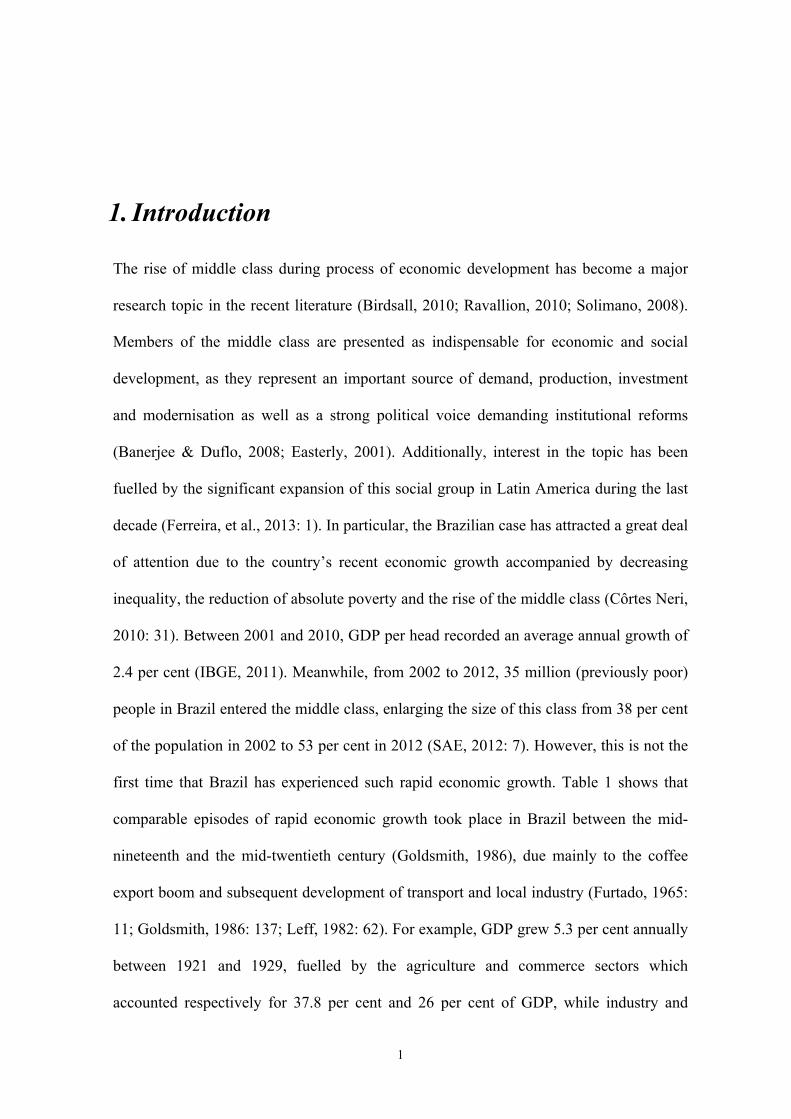
Abstract This article investigates the rise of the middle class in Brazil between the mid-nineteenth and mid-twentieth centuries and its connection with inequality. To this purpose Brazil’s income distribution is explored from two dimensions: inequality and polarisation. A new middle class index (MCI), based on polarisation methods, is used to assess the evolution of the middle class in terms of both income and status. Results suggest that during the nineteenth century low income levels prevented the achievement of high inequality values and the emergence of a middle class. Then in the early twentieth century Brazil experienced a process of economic growth accompanied by increasing inequality in a Kuznetsian sense in which the middle class arose. Yet, despite rapid economic growth during the following decades, the continued increase of inequality, especially between 1930 and 1950, impeded the consolidation of the middle class and the reduction of poverty. JEL classification: D31, D63, N16, N36, O15. Keywords: Middle class, inequality, polarisation, Brazil.
This study has been developed with the financial support of Universidad Carlos III de Madrid through the PIF fellowship. I am thankful to Prof. Leandro Prados de la Escosura for crucial guide and support. I am indebted to Prof. Carlos Gradín for his help with the EGR index. Observations and suggestions on the methodological part from Diego Battistón and Alfonso Herranz-Loncán were most appreciated. I am also indebted to Henry Willebald and Leonardo Monasterio who kindly shared their data. Special thanks are due to Alejandra Irigoin and Prof. Jeffrey Williamson for their valuable comments on my work. I am the only responsible for its errors. * María Gómez León: Dpto de Ciencias Sociales, Universidad Carlos III de Madrid, Email: [email protected]
Notice The material presented in the EHES Working Paper Series is property of the author(s) and should be quoted as such.
The views expressed in this Paper are those of the author(s) and do not necessarily represent the views of the EHES or its members
"
1
1. Introduction
The rise of middle class during process of economic development has become a major
research topic in the recent literature (Birdsall, 2010; Ravallion, 2010; Solimano, 2008).
Members of the middle class are presented as indispensable for economic and social
development, as they represent an important source of demand, production, investment
and modernisation as well as a strong political voice demanding institutional reforms
(Banerjee & Duflo, 2008; Easterly, 2001). Additionally, interest in the topic has been
fuelled by the significant expansion of this social group in Latin America during the last
decade (Ferreira, et al., 2013: 1). In particular, the Brazilian case has attracted a great deal
of attention due to the country’s recent economic growth accompanied by decreasing
inequality, the reduction of absolute poverty and the rise of the middle class (Côrtes Neri,
2010: 31). Between 2001 and 2010, GDP per head recorded an average annual growth of
2.4 per cent (IBGE, 2011). Meanwhile, from 2002 to 2012, 35 million (previously poor)
people in Brazil entered the middle class, enlarging the size of this class from 38 per cent
of the population in 2002 to 53 per cent in 2012 (SAE, 2012: 7). However, this is not the
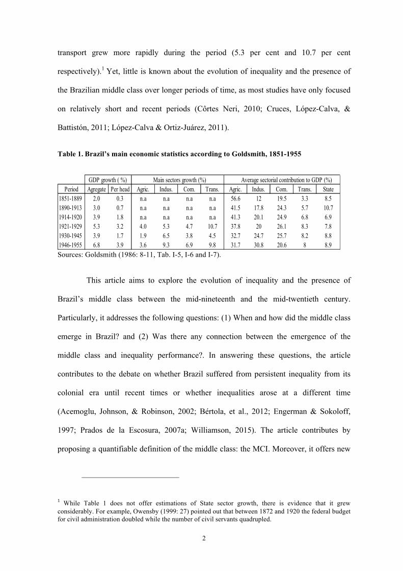
first time that Brazil has experienced such rapid economic growth. Table 1 shows that
comparable episodes of rapid economic growth took place in Brazil between the mid-
nineteenth and the mid-twentieth century (Goldsmith, 1986), due mainly to the coffee
export boom and subsequent development of transport and local industry (Furtado, 1965:
11; Goldsmith, 1986: 137; Leff, 1982: 62). For example, GDP grew 5.3 per cent annually
between 1921 and 1929, fuelled by the agriculture and commerce sectors which
accounted respectively for 37.8 per cent and 26 per cent of GDP, while industry and
"
2
transport grew more rapidly during the period (5.3 per cent and 10.7 per cent
respectively).1 Yet, little is known about the evolution of inequality and the presence of
the Brazilian middle class over longer periods of time, as most studies have only focused
on relatively short and recent periods (Côrtes Neri, 2010; Cruces, López-Calva, &
Battistón, 2011; López-Calva & Ortiz-Juárez, 2011).
Table 1. Brazil’s main economic statistics according to Goldsmith, 1851-1955
Sources: Goldsmith (1986: 8-11, Tab. I-5, I-6 and I-7).
This article aims to explore the evolution of inequality and the presence of
Brazil’s middle class between the mid-nineteenth and the mid-twentieth century.
Particularly, it addresses the following questions: (1) When and how did the middle class
emerge in Brazil? and (2) Was there any connection between the emergence of the
middle class and inequality performance?. In answering these questions, the article
contributes to the debate on whether Brazil suffered from persistent inequality from its
colonial era until recent times or whether inequalities arose at a different time
(Acemoglu, Johnson, & Robinson, 2002; Bértola, et al., 2012; Engerman & Sokoloff,
1997; Prados de la Escosura, 2007a; Williamson, 2015). The article contributes by
proposing a quantifiable definition of the middle class: the MCI. Moreover, it offers new
1" While Table 1 does not offer estimations of State sector growth, there is evidence that it grew considerably. For example, Owensby (1999: 27) pointed out that between 1872 and 1920 the federal budget for civil administration doubled while the number of civil servants quadrupled."
GDP growth ( %) Main sectors growth (%) Average sectorial contribution to GDP (%)Period Agregate Per head Agric. Indus. Com. Trans. Agric. Indus. Com. Trans. State
1851-1889 2.0 0.3 n.a n.a n.a n.a 56.6 12 19.5 3.3 8.51890-1913 3.0 0.7 n.a n.a n.a n.a 41.5 17.8 24.3 5.7 10.71914-1920 3.9 1.8 n.a n.a n.a n.a 41.3 20.1 24.9 6.8 6.91921-1929 5.3 3.2 4.0 5.3 4.7 10.7 37.8 20 26.1 8.3 7.81930-1945 3.9 1.7 1.9 6.5 3.8 4.5 32.7 24.7 25.7 8.2 8.81946-1955 6.8 3.9 3.6 9.3 6.9 9.8 31.7 30.8 20.6 8 8.9
"
3
insights on the relationship between inequality, the reduction of absolute poverty and the
rise of the middle class.
The paper’s main findings can be summarised as follows. Principally, the paper
shows that Brazil’s inequality is not endemic and that the idea of a middle social group
(different from the wealthy landowners and the servile class) existing between the mid-
nineteenth and mid-twentieth centuries is not remote. During the nineteenth century
Brazil exhibited low inequality values linked to low income levels, which, in turn,
impeded the rise of its middle class. Then, from the early twentieth century the process of
economic growth, accompanied by increasing inequality, went hand in hand with the
emergence of the middle class. Yet, in the following decades, despite rapid economic
growth, the continued increase of inequality, especially from the Vargas Era, inhibited the
consolidation of the middle class and the eradication of poverty.
The article proceeds as follows: Section 2 offers a short discussion on Brazil’s
inequality from 1839 and 1950; I then analyse Brazil’s income distribution during this
period from a polarisation approach and introduce the new MCI based on polarisation
measures (Section 3).2 I show the sources I used for the MCI estimation in Section 4, and
analyse the performance of the middle class between 1839 and 1950 in terms of income
(Section 5) and in terms of status (Section 6). Finally, Section 7 concludes.
2 The choice of 1839 as the beginning of the period responds to the interest in investigating Brazil’s income distribution from the earlier available year right after Brazil’s independence (in 1822). "
"
4
2. A glance at inequality challenging the over-pessimistic
Studies on economic development have been usually worried about the connection
between persistent inequality and poverty (Birdsall & Londoño, 1997; Bourguignon,
2000; Ravallion, 2001). Yet little has been said about the relationship between inequality
and a key factor to achieve economic and social development: the rise of the middle
class. Tentatively, by looking at inequality performance one might obtain some intuitions
on the middle class emergence and evolution. In particular, quantitative works using the
Gini index might be especially useful for this purpose, as the Gini index has the
characteristic of being particularly sensitive to transfers in the central part of the
distribution.
In this regard, the examination of the literature on Brazil’s historical inequality
highlights two different stories: a pessimistic one, in which persistent high inequality in
Brazil would have made unlikely the existence of any social group different from the
wealthy landowners and a poor servile class; and a more optimistic one, in which the
existence of inequality would not have been endemic and the presence of different social
groups not so improbable.
In the negative view, inequality would be rooted in Brazilian colonial history.
Engerman and Sokoloff (1997) argued that the roots of Latin America inequality are
located in the natural resource endowments that fostered the development of extractive
institutions, which, in turn, undermined growth. Acemoglu, Johnson and Robinson
(2002), while also pointing at the presence of extractive institutions as the main reason
for persistent inequality in Latin America, held, however, that extractive institutions
originated due to the abundant population density and affluence. According to this view,
"
5
quantitative estimations from Bértola et al., (2012) suggest that inequality was already
high by 1870, with a Gini coefficient higher than 0.5 that continued increasing during the
first globalisation boom.
From a more optimistic perspective, quantitative explorations by Prados de la
Escosura (2007a), Milanovic, Lindert, and Williamson (2010) –MLW hereafter-, and
Williamson (2010) suggest that Brazil’s inequality persistence is a “myth” as inequality
did not begin to rise until a decade or two before the start of the belle époque (1870-1914)
(Williamson, 2010; 2015) or even later, from 1913 onwards according to Gini
coefficients below 0.5 (Prados de la Escosura, 2007a). To these authors low inequality
values resulted from low levels of income per head.
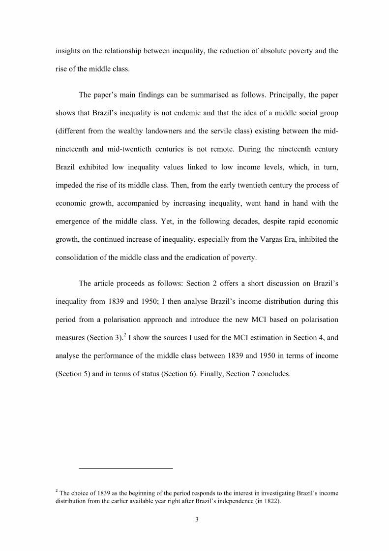
The findings of this article tend to agree with this hypothesis of low inequality
levels associated with low income values, with estimated Gini coefficients ranging
between 0.2 and 0.35. Indeed, as can be seen in Figure 1, my estimates are very close to
those reported by Prados de la Escosura (2007a) even though we use independent
sources.3 Both show a long-run decline in inequality until 1913, which was interrupted by
a flat phase between the 1870s and the 1890s according to Prados de la Escosura’s
(2007a) estimates, or by a short-lived increase from 1860s to 1870s according to my
estimates. However, both estimates then report a sharp increase in inequality from 1913
onwards.
3 Prados de la Escosura (2007a) calculated Pseudo-Ginis by backcasting actual Gini estimates with the ratio between real GDP per worker and unskilled real wage rates, expressed in index. He relies on Williamson’s ([1995] 1996) real wages for the case of Brazil, whereas my Gini estimations come from own calculations based on the sources presented in Section 4.
"
6
Figure 1. Brazil’s inequality: Gini coefficients Sources: Prados de la Escosura (2007a: 296, Tab.12.1); MLW (2010: 63, Tab.2) and Bértola et al. (2012: 12, Tab.6). Own estimates are detailed in Section 4.
At this point, I would like to introduce Milanovic’s approach as a way to test how
plausible these estimates are. This author claims that when: “there is a society with an
average income just slightly above the subsistence minimum. If all members of the
society are to survive, then the surplus [the extraction ratio], even if it is appropriated by
a tiny group of people, cannot be large, and the Gini coefficient must be relatively low”
(Milanovic 2006: 466-67).
He further argued for the existence of a maximum attainable inequality (which is
an increasing function of mean overall income) which can be estimated and represented
by the Inequality Possibility Frontier (IPF henceforth).4 Then, let’s place the different
estimates within the proposed IPF, based on GDP per head (in 1990$PPP) from
Maddison (2003).
4 These concepts are also used in MLW (2007; 2010); and Milanovic (2006; 2009; 2011).
0.2
0.3
0.4
0.5
0.6Gini
1840 1850 1860 1870 1880 1890 1900 1910 1920 1930 1940 1950Year
Bértola, et al.,(2012) MLW (2010)
Gómez León Prados de la Escosura (2007a)
"
7
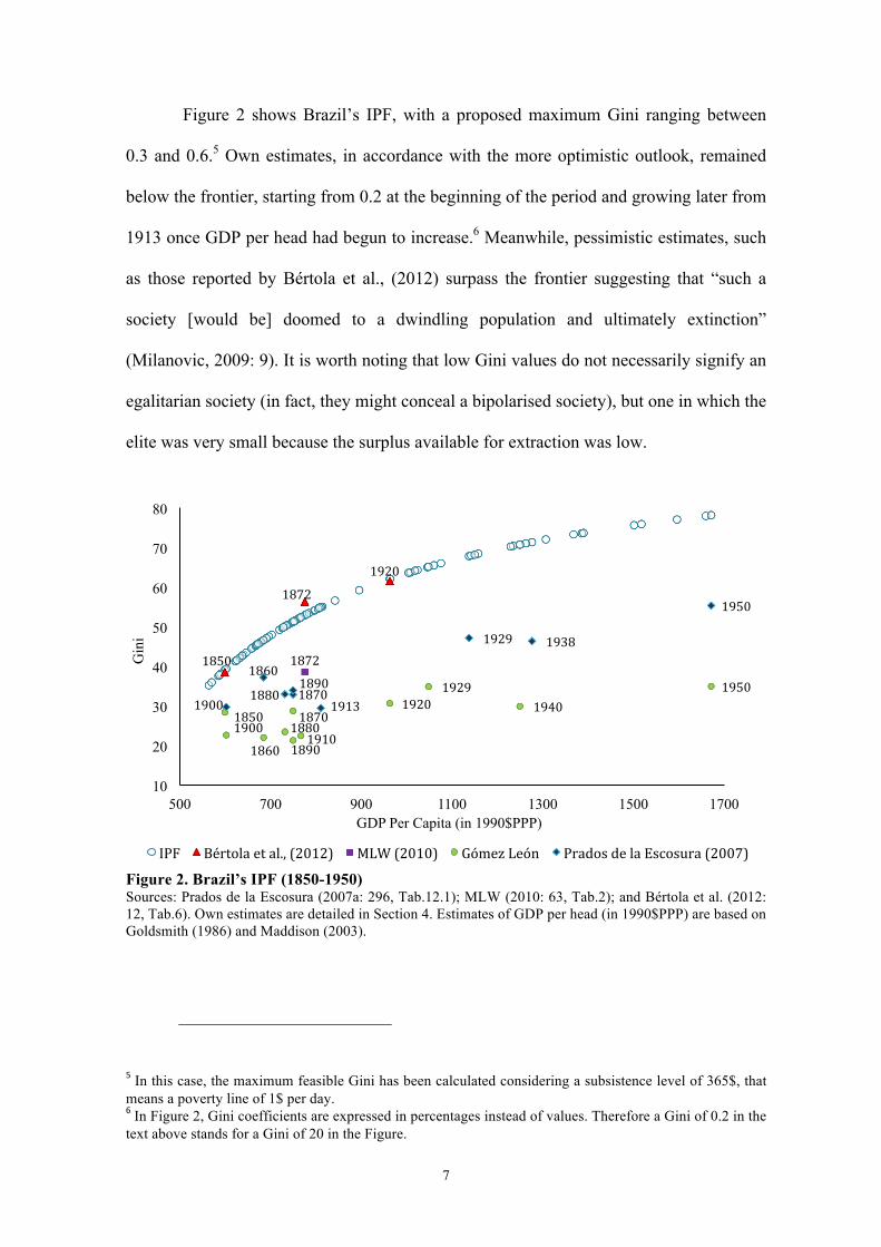
Figure 2 shows Brazil’s IPF, with a proposed maximum Gini ranging between
0.3 and 0.6.5 Own estimates, in accordance with the more optimistic outlook, remained
below the frontier, starting from 0.2 at the beginning of the period and growing later from
1913 once GDP per head had begun to increase.6 Meanwhile, pessimistic estimates, such
as those reported by Bértola et al., (2012) surpass the frontier suggesting that “such a
society [would be] doomed to a dwindling population and ultimately extinction”
(Milanovic, 2009: 9). It is worth noting that low Gini values do not necessarily signify an
egalitarian society (in fact, they might conceal a bipolarised society), but one in which the
elite was very small because the surplus available for extraction was low.
Figure 2. Brazil’s IPF (1850-1950) Sources: Prados de la Escosura (2007a: 296, Tab.12.1); MLW (2010: 63, Tab.2); and Bértola et al. (2012: 12, Tab.6). Own estimates are detailed in Section 4. Estimates of GDP per head (in 1990$PPP) are based on Goldsmith (1986) and Maddison (2003).
5"In this case, the maximum feasible Gini has been calculated considering a subsistence level of 365$, that means a poverty line of 1$ per day."6"In Figure 2, Gini coefficients are expressed in percentages instead of values. Therefore a Gini of 0.2 in the text above stands for a Gini of 20 in the Figure."
1850%
1872%
1920%
1872%
1850%
1860%
1870%1880%1890%
1900%1910%
1920%%
1929%1940%
1950%1860%
1870%1880%1890%
1900% 1913%
1929% 1938%
1950%
10
20
30
40
50
60
70
80
500 700 900 1100 1300 1500 1700
Gin
i
GDP Per Capita (in 1990$PPP)
IPF% Bértola%et%al.,%(2012)% MLW%(2010)% Gómez%León% Prados%de%la%Escosura%(2007)%
"
8
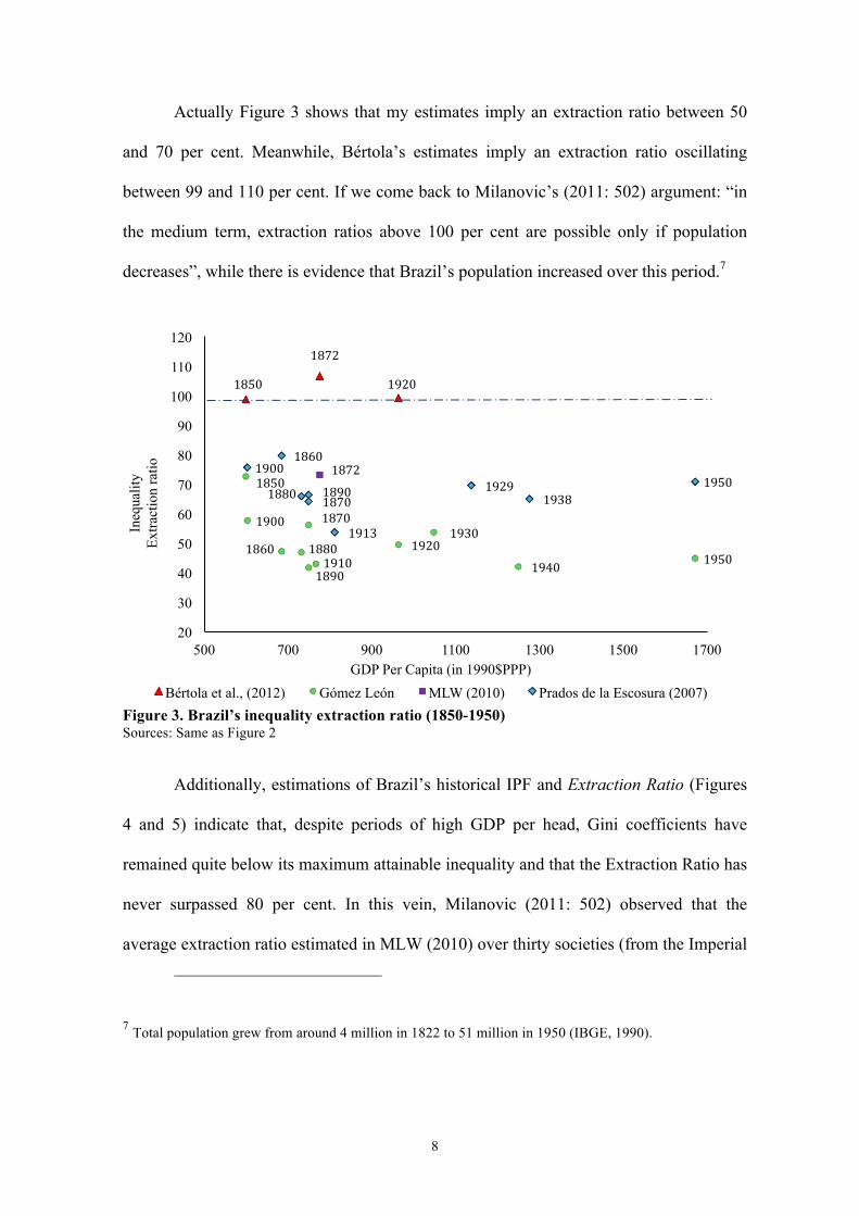
Actually Figure 3 shows that my estimates imply an extraction ratio between 50
and 70 per cent. Meanwhile, Bértola’s estimates imply an extraction ratio oscillating
between 99 and 110 per cent. If we come back to Milanovic’s (2011: 502) argument: “in
the medium term, extraction ratios above 100 per cent are possible only if population
decreases”, while there is evidence that Brazil’s population increased over this period.7
Figure 3. Brazil’s inequality extraction ratio (1850-1950) Sources: Same as Figure 2
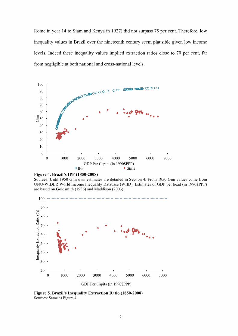
Additionally, estimations of Brazil’s historical IPF and Extraction Ratio (Figures
4 and 5) indicate that, despite periods of high GDP per head, Gini coefficients have
remained quite below its maximum attainable inequality and that the Extraction Ratio has
never surpassed 80 per cent. In this vein, Milanovic (2011: 502) observed that the
average extraction ratio estimated in MLW (2010) over thirty societies (from the Imperial
7 Total population grew from around 4 million in 1822 to 51 million in 1950 (IBGE, 1990).
"
1850%
1872%
1920%
1850%
1860%
1870%%
1880%
1890%
1900%
1910%1920%
1930%
1940% 1950%
1872%1860%
1870%1880% 1890%
1900%
1913%
1929%1938%
1950%
20
30
40
50
60
70
80
90
100
110
120
500 700 900 1100 1300 1500 1700
Ineq
ualit
y
Extra
ctio
n ra
tio
GDP Per Capita (in 1990$PPP)
%Bértola et al., (2012) Gómez León MLW (2010) Prados de la Escosura (2007)
"
9
Rome in year 14 to Siam and Kenya in 1927) did not surpass 75 per cent. Therefore, low
inequality values in Brazil over the nineteenth century seem plausible given low income
levels. Indeed these inequality values implied extraction ratios close to 70 per cent, far
from negligible at both national and cross-national levels.
Figure 4. Brazil’s IPF (1850-2008) Sources: Until 1950 Gini own estimates are detailed in Section 4; From 1950 Gini values come from UNU-WIDER World Income Inequality Database (WIID). Estimates of GDP per head (in 1990$PPP) are based on Goldsmith (1986) and Maddison (2003).
Figure 5. Brazil’s Inequality Extraction Ratio (1850-2008) Sources: Same as Figure 4.
0
10
20
30
40
50
60
70
80
90
100
0 1000 2000 3000 4000 5000 6000 7000
Gin
i
GDP Per Capita (in 1990$PPP) IPF% Ginis%
20
30
40
50
60
70
80
90
100
0 1000 2000 3000 4000 5000 6000 7000
Ineq
ualit
y Ex
tract
ion
Rat
io (%
)
GDP Per Capita (in 1990$PPP)
"
10
To sum up, inequality trends might be interpreted as supportive of the presence of
a middle class over the period 1850-1950, especially up to 1913 (when Gini coefficients
were falling) with a reversal thereafter. The alternative interpretation could be, however,
that low inequality values in the nineteenth century, pointing to low income levels, might
have prevented the emergence of the middle class. Yet, the opposite could have happened
during the twentieth century, when high inequality values could be linked to an early
phase of economic growth in a Kuznetsian sense (i.e. to the transitional process from the
traditional sector to a modern one), allowing for the appearance of different social groups.
Therefore, inferences on the middle class’ performance based on inequality measures are
far from being conclusive, and thus a complementary analysis must be applied.
3. Defining the middle class through polarisation measures
An alternative to study and clarify the presence of the middle class is to examine the
income distribution from a polarisation approach. The key idea behind this method is
that, contrary to inequality, polarization measures control for the existence of specific
social groups, such as the middle class. This is because while inequality measures (such
as Gini) estimate the extent of concentration of the population around the mean income of
the distribution, polarisation measures test the formation of different groups of income
along this distribution. Therefore, whereas with inequality measures distributions follow
unimodal shapes, polarisation measures lead to distributions with bimodal (or
multimodal) shapes which allow the clear discernment of the absence (or presence) of a
middle class (Gradín & del Río, 2001: 4). In this sense, from a polarisation perspective,
"
11
the extreme situation arises when the population is equally distributed between two
distant poles (bipolarised distributions), highlighting the absence of a middle class.8
Following this reasoning, Foster and Wolfson (2010) examined the lack of the
middle class by developing a bipolarisation index (hereafter FW index). This index
assumed the existence of two equally sized groups whose cut-off is the median income.9
Therefore, for these authors, the increase in the FW index (i.e. the increase in
bipolarization) indicated the disappearance of the middle class, while the fall of the index
suggested the contrary: the rise of the middle class.
Later on, this idea was subsequently taken to the next level by Cruces, López-
Calva and Battistón (2011) in their study of the Latin American middle class. These
authors started from a tripolarisation situation; that is, assuming the existence of three
income groups. Hence, for these authors it was the increase of the tripolarisation indicator
that indicated the rise of the middle class. In this case, since they assumed the existence
of three income groups from the beginning, they calculated tripolarisation by using the
polarisation index developed by Esteban Gradín and Ray (2007) (EGR index hereafter)
which, contrary to the FW index, allows for the existence of n different sized groups.
Following this reasoning, (Foster & Wolfson, 2010; Cruces, López-Calva, &
Battistón, 2011), it is crucial to understand that decreasing bipolarisation together with
increasing tripolarisation clearly point to the emergence of a middle class. Therefore, a
step further with regard to the definition of the middle class would be introducing a new
8" From an inequality perspective instead, a situation of extremity would be reached when one person receives all the income and the rest receives nothing (distribution with a long right tail).""9 This polarisation index is derived from the Lorenz curve and it can be defined as: twice the area of the region between the Lorenz curve and the tangent line. For further details see Foster & Wolfson (2010).
"
12
middle index (MCI), which is defined as the ratio between tripolarisation and
bipolarisation.
The rationale behind this definition is that the separate analysis of bipolarisation
and tripolarisation might lead to inaccurate conclusions when they move alongside each
other. For example, Figure 6 shows the evolution of both tripolarisation and
bipolarisation in Brazil between 1839 and 1950. As can be observed, throughout the
nineteenth century both indicators moved together making it difficult to conclude when
the middle class arose. For instance, when looking at bi-polarisation trends one could
place the emergence of the middle class in the early nineteenth century, when bi-
polarisation was falling. Tri-polarisation, however, was falling too. Similarly, in terms of
tri-polarisation, one could place the rise of the middle class in the 1860s, when tri-
polarisation increased. Yet so did bipolarisation. Meanwhile, if one analyses both
indicators together, it can be presumed that increases in tri-polarisation along with
decreases in bi-polarisation are what undoubtedly should be indicating the emergence of
a middle class.
Figure 6. Brazil 1839-1950: Bipolarisation (EGR, n=2) and Tripolarisation (EGR, n=3), 5- year moving averages. Sources: From 1839 to 1930 based on Bértola et al., (2007), Monasterio (n.d), DGE (1872, 1926) and Lobo (1978: 803-20); for 1940 and 1950 sources are IBGE (1990) and DGE (1950, 1956).
0.04
0.06
0.08
0.10
0.12
0.14
0.16
1839 1849 1859 1869 1879 1889 1899 1909 1919 1929 1939 1949
EGR
inde
x (n
=3 a
nd n
=2)
Year%Tripolarisation Bipolarisation
"
13
At this point, it might be argued that merely examining tripolarisation and testing
the size of the middle income group would provide enough evidence of the presence of
the middle class. However, just looking at the size of the middle income group can lead
to incorrect conclusions when this group is actually very similar to the poorer one in
terms of income. For instance, Milanovic (2009: 7) argued that: “in preindustrial societies
the middle [in terms of income] was not much different from the bottom”. Therefore, in
order to avoid incorrect inferences when reporting the presence of a middle class, it is
crucial to consider those situations in which the phenomenon tripolarisation surpasses
bipolarization, meaning that there is a middle income group homogeneous inside and
different from the other two.10
Importantly, the proposed new MCI, defined as the ratio between tripolarisation
and bipolarization, permits one to capture this phenomenon. When tripolarisation
overcomes bipolarization, the MCI will be above one, reporting the presence of a middle
class. Meanwhile when bipolarisation is equal or higher than tripolarisation, the MCI will
be equal or below one, suggesting the opposite: the lack of a middle class.
Finally, since the purpose of this article is to find as much accurate definition as
possible of the Brazilian middle class, I will address two dimensions of the middle class:
income and status. Hence, I will construct two MCIs: one based on polarisation measures
in terms of income, and the other based on polarisation measures in terms of status. Both
10 Note that tripolarisarion is a particular case of bipolarisation, which arises when one of the two groups (the high or the low) has become heterogeneous inside (in terms of income) giving rise to the emergence of a new middle income group. In the same vein, bipolarisation is a particular case of tripolarisation, which increases when two of the three groups have merged because both have become similar in terms of income.
"
"
14
exercises are explained in the following sub-sections and empirically tested in Sections 5
and 6.
3.1 Defining middle class in terms of income
First, in order to define the middle class in terms of income, I calculate the MCI using the
EGR polarization measure. The choice of the EGR measure derives from the fact that it
allows for the estimation of polarization for n groups. In addition, the EGR avoids
arbitrariness in the definition of groups, as the cut-offs are set endogenously. For a better
understanding of this, in what follows, I explain the main characteristics of this index.
The EGR index consists of a general polarisation measure with four
characteristics: (1) a high degree of homogeneity within each group; (2) a high degree of
heterogeneity between groups; (3) a small number of significant sized groups, meaning
that very small groups (such as isolated individuals) have little weight; and (4) the higher
the number of selected groups, the lower the polarisation.
In particular, this index is based on a model of individual perceptions according to
two factors: the identification factor and the alienation factor. The identification factor
refers to how the individual feels in respect to other individuals, considered to be
members of this group in terms of income. The alienation factor captures how an
individual feels with respect to the rest of individuals that belong to other groups. The
joining of both factors composes the effective antagonism feeling of each individual.
Finally, the aggregation of the effective antagonism feelings of all members in society
"
15
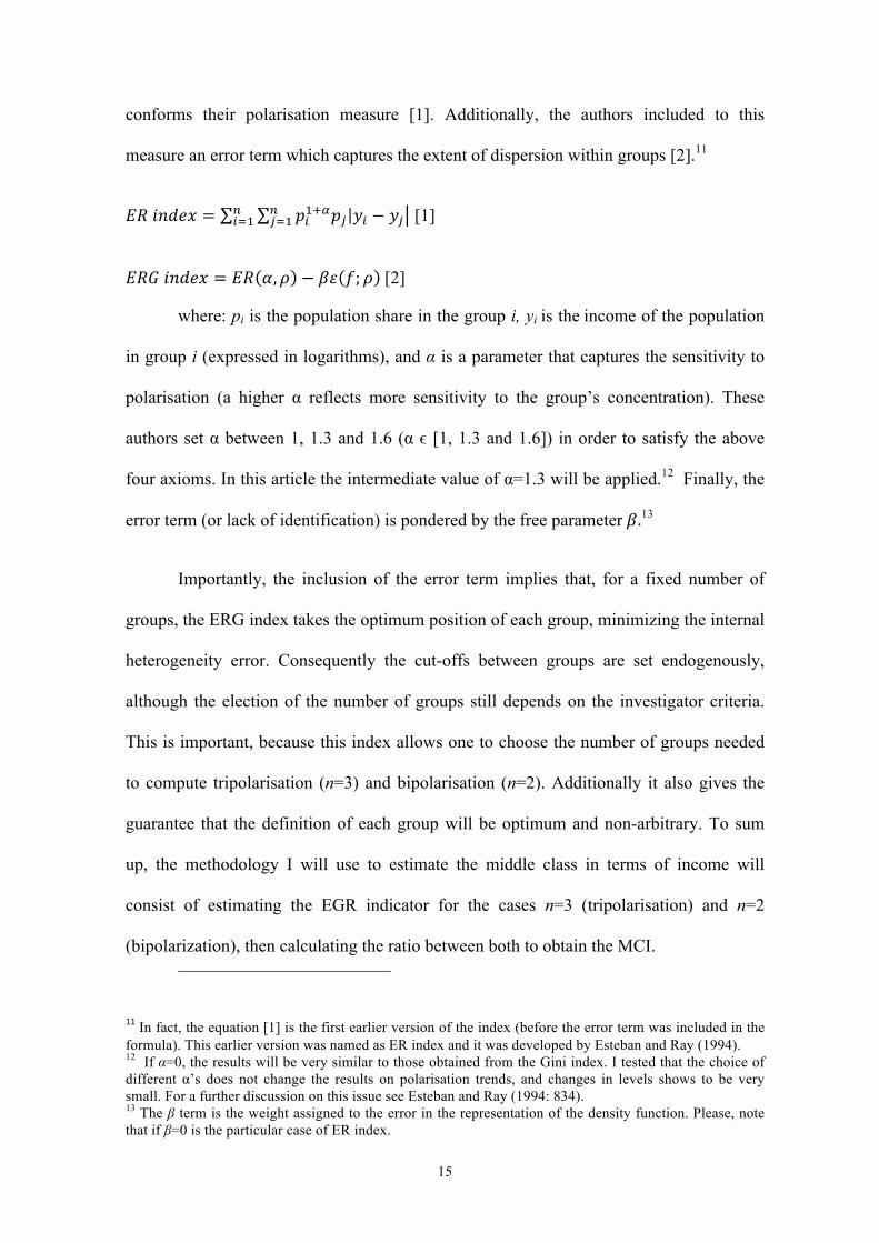
conforms their polarisation measure [1]. Additionally, the authors included to this
measure an error term which captures the extent of dispersion within groups [2].11
!"!!"#$% = !!!!!!! !! − !!!!!!
!!!! [1]
!"#!!"#$% = !" !,! − !" !;! ![2]
where: pi is the population share in the group i, yi is the income of the population
in group i (expressed in logarithms), and α is a parameter that captures the sensitivity to
polarisation (a higher α reflects more sensitivity to the group’s concentration). These
authors set α between 1, 1.3 and 1.6 (α ϵ [1, 1.3 and 1.6]) in order to satisfy the above
four axioms. In this article the intermediate value of α=1.3 will be applied.12 Finally, the
error term (or lack of identification) is pondered by the free parameter!!.13
Importantly, the inclusion of the error term implies that, for a fixed number of
groups, the ERG index takes the optimum position of each group, minimizing the internal
heterogeneity error. Consequently the cut-offs between groups are set endogenously,
although the election of the number of groups still depends on the investigator criteria.
This is important, because this index allows one to choose the number of groups needed
to compute tripolarisation (n=3) and bipolarisation (n=2). Additionally it also gives the
guarantee that the definition of each group will be optimum and non-arbitrary. To sum
up, the methodology I will use to estimate the middle class in terms of income will
consist of estimating the EGR indicator for the cases n=3 (tripolarisation) and n=2
(bipolarization), then calculating the ratio between both to obtain the MCI.
11"In fact, the equation [1] is the first earlier version of the index (before the error term was included in the formula). This earlier version was named as ER index and it was developed by Esteban and Ray (1994)."12 If α=0, the results will be very similar to those obtained from the Gini index. I tested that the choice of different α’s does not change the results on polarisation trends, and changes in levels shows to be very small. For a further discussion on this issue see Esteban and Ray (1994: 834). 13 The β term is the weight assigned to the error in the representation of the density function. Please, note that if β=0 is the particular case of ER index.
"
16
3.2 Defining middle class in terms of status
In order to define the middle class in term of status, it is necessary to apply a polarization
measure based on characteristics; this is a measure that permits to set groups according to
any attribute, in this case the status. In particular, I calculate the MCI in terms of status
using the polarization indicator in terms of characteristics developed by Zhang and
Kanbur (2001) (ZK index hereafter).
The ZK index is an indicator based on the inequalities within and between groups,
derivatives from Theil’s (1979) generalized entropy index, according to some
characteristic (such as gender, education, ethnicity, etc.). In other words, this indicator
analyses the distance among groups linked to differences within groups, according to any
attribute (for example the status). In this sense, the more homogenous the groups are
(meaning less inequality within groups), the bigger the differences existing between
groups will be (that is, more inequality between groups) and the bigger the polarisation.
Therefore the ZK polarisation index is defined as the ratio between GE[0] between and
GE[0] within, which respectively capture the inequality between groups and the
inequality within groups according to the general entropy inequality index.14
In this article, when using the ZK index, the alienation factor (what determines
differences across groups) will be income, while the identification factor (what
determines homogeneity within the group) will be status. In this vein, it should be noted
that while with the EGR the groups were set endogenously, with the ZK index the groups
must be previously defined according to specific characteristics (in this case, the status).
In the same vein, it is also worth noting that, contrary to the EGR (2007) index, in the ZK
14"For a review of how the generalized entropy index is constructed see Theil (1979)"
"
17
(2001) index the size of groups remains fixed. Thus, given a fixed active population
structure, it is the case that tripolarisation is always higher than bipolarisation, so
presumably the MCI in terms of status will be always above one. Yet, the evolution of the
middle class in terms of status still can be assessed by looking at the r evolution of the
ratio between tripolarisation and bipolarisation.
Notably, while it can be argued that the prior definition of groups implies a certain
level of arbitrariness, the differentiation of groups in terms of characteristics is not as
controversial as it can be in terms of income. For example, there is evidence that in
Brazil’s nineteenth and twentieth centuries some characteristics such as being a cultivated
person or having a non-manual job, identified people with the middle class status more
than their incomes did (Owensby, 1999). Therefore, in this case, I form the groups
according to the social status linked to the profession.
The criteria when assigning a particular status to the different professional
categories is based on the Historical International Social Class Scheme (HISCLASS
hereafter) classification, which is linked, in turn, to the Historical International Standard
Classification of Occupations (HISCO hereafter) classification. The link between the
HISCLASS and HISCO classification is established according to the skill level of each
profession (high, medium or low) and its condition (manual or non-manual).15 While
HISCLASS grouped the classified occupations into twelve classes (ranked on a prestige
or status scale), I have grouped and ranked them into three different groups (high, middle
15""See van Leeuwen, et al. (2002)"and van Leeuwen and Maas (2011)."
"
18
and low) and two groups (high and low) which will allow me to fully calculate
tripolarisation and bipolarisation, thus the MCI in terms of status.16
In summary, to define the Brazilian middle class in terms of status, I calculate the
ZK (2001) for the cases n=3 and n=2, then the ratio between these two to obtain the MCI
in terms of status. In this case, arbitrariness when defining groups is not just ineluctable
but also necessary, as the groups need to be previously distinguished according to
professional status.
4. Data analysis
The first household survey developed in Brazil dates from 1967, making this approach
unpractical for the historical purpose of this article. Therefore, to explore Brazil’s income
distribution, I have recurred to the construction of a social table with information on the
structure of active population (by profession) and associated real income, distinguishing
by gender (male, female), condition (free, slave) and area (urban, rural).
First, to obtain data on active population by profession I turned into national
censuses. In Brazil the first national census corresponds to 1872 and the subsequent
censuses were conducted in 1920, 1940 and 1950 (DGE-Diretoria Geral de Estatística,
1872; 1926; 1950; 1956). Since there is not an annual series on active population data, I
apply the fixed structure of the active population provided in the censuses to my income
time series (Bértola et al., 2007).17 From 1839 to 1898 I use the census of 1872; from
16"See Appendix Table 1. 17"While interpolation methods could have been applied from 1870 to 1950 to the data on total population, lack of data from 1839 to 1870 did not allow me to maintain a uniform criterion. Therefore, I decided to maintain the same methodology for my whole period, using the fixed active population provided in the census benchmark years.
"
19
1899 to 1930 the 1920 census; and for 1940 and 1950 the censuses developed for these
single years. Secondly, the data for the income time series for each professional category
is taken from the censuses (DGE 1872, 1926, 1950, 1956), but also from historical
statistics (IBGE 1990) and official information on yearly nominal wages provided by
Lobo (1978).18 Moreover, Lobo’s dataset has been complemented with additional
information of yearly incomes of landowners and slaves.19
I have paid attention to the fact that from 1839 to 1898 most income information
belongs to Rio de Janeiro and other regions of South-Eastern Brazil. Hence, the time
series of active population (by profession) has been constructed using information on the
active population (provided by the 1872 census) present in the South-Eastern Brazil
(Espírito Santo, Minas Gerais, Municipio Neutro, Rio de Janeiro and São Paulo). Yet
there are some good grounds to believe that the sample is representative as in 1920 more
than half of the urban population resided in Rio de Janeiro and in São Paulo (Fausto,
1989: 234). Moreover, almost 75 per cent of total GDP was concentrated in the South-
Eastern and Southern regions by 1872, and this percentage increased during the first
decades of the twentieth century due to the expansion of the south (Bértola et al. 2007:
3).20 Data aggregation for 1872 results in a population of around 4 million (with a total
18 In Lobo (1978) wages are presented as yearly averages. For the estimation, she uses wage rates per hour (8 hours per day, 200 hours per month). In this paper, yearly averages have been multiplied by 12 (months) in order to obtain wages per year and make them comparable to the yearly income information presented by other sources. 19 Slave income estimations provided by Willebald are set according to the cost of feeding slaves in mining companies, plus a similar amount that covered clothing and housing expenses. Estimations for landowners’ income are based on data kindly provided by Willebald and Monasterio. 20" It should be noted that the reality in the North was quite different to the South-East. For example, in terms of the IPF (described in Section 2), it could be suggested that by the end of the period the North region was most likely characterized by values of income and inequality close to those shown in the late-nineteenth century."
"
20
population of 9.6 million), distributed across 36 different professional categories.21
Moreover, the 1872 census includes information on of the active population gender (male
or female) and the labour condition (slave or free). In this case, female income has been
estimated as 60 per cent of the male one (either slaves or free).22 Moreover, it is
important to stress that while in Brazil the end of slavery came with the “Lei Áurea” of
1888, the status of past slaves did not change directly (Owensby, 1999: 41) and neither
did their mean income and hence the 1872 census includes slave records until 1898.23
Next, from 1899 to 1930, the mean income time series has been constructed using
the same income resources as in the previous period, but it has been assigned to a fixed
structure of the active population according to the 1920 census. In 1920, the demographic
census also offers information on gender. However, this census does not provide
aggregate data at the country level, nor at the state level, but disaggregated information
by municipalities. Due to the large number of municipalities (1,304 in the entire country
and 430 in the South-East region) a selection of the sample has been chosen.24 The data
aggregation is carried out on a sample of an active population with 7.8 million individuals
(of a total population of 27 million) also distributed across 36 different professions.
Additionally, in order to take into account wage differences throughout the
country, I have considered differences between rural and urban areas. Here Lobo (1978)
21 From the total observations only 2,268,208 could be considered as “active”. The other 1,737,593 observations belong to the “without a profession” category. Nevertheless, since these people could be working in the informal market, average income estimations (based on low income professional categories such as hairdressing and caretaking) have also been assigned to this group. 22"Estimations based on the wages differential between male and female have been calculated from the DGE (1926)."23 There is evidence that once the free labor system was established, “darker skinned people tended disproportionately to work at manual jobs [whereas] the white or near-white men […] benefited from racial cleavages and assumptions in hiring, promotion, housing, patronage, social contracts and education” (Owensby, 1999: 41). 24 The choice has been to take the most populated municipalities (183 of 430) belonging to the States of the South-Eastern region: Minas Gerais (68 of 178), São Paulo (37 of 48) and Rio de Janeiro (78 of 204).
"
21
provides nominal urban wages and I have estimated the rural nominal salaries for the 36
professional categories and the proportion of population (by profession) in rural and
urban areas. For this purpose, I have employed Klein (1995: 538, Tab.7) and Nunes’
(2003: 334, Tab.13) works and Monasterio’s data.25 These sources provide information
on the income declared in the electoral rolls, including voters’ profession and their area of
residence (distinguishing between urban and rural parishes). With this information I have
estimated the differences between urban and rural wages (by profession) and the
proportion of people (also by profession) residing in one area or another. Therefore,
nominal wages were deflated until 1930 by the consumer price index provided by Lobo
(1978: 95-99, Tab.4.43).26
For the years 1940 and 1950, both the active population (by profession) and the
linked mean income by professional category come from the censuses (DGE 1950, 1956)
and from the IBGE (1990). The information has been compiled at country level. It
comprises an active population with 15 million individuals (of a total population of 41
million) in 1940, and with 25 million individuals (of a total population of 51 million) in
1950, distributed across 22 professional categories. As in the previous period, nominal
salaries have been deflated, using the price index provided by Onody (1960: 118) liaised
to the Lobo’s ones.27
25 Klein (1995) and Nunes (2003) provide information for São Paulo, while Monasterio does for Rio Grande do Sul. The estimations obtained for São Paulo and Rio Grande do Sul have been compared with those obtained for the city of Rio de Janeiro, provided by the DGE (1895). Results are very similar, so it seems possible to use the same estimations along the South-Eastern region. 26 This index is introduced in Lobo (1978). It is based on the consumption basket elaborated by Affonseca (1920) in 1919. This basket reported middle-high class consumption habits (for example, the food weighs were attributed according their importance on the basket of a middle-high class family). For the years 1940 and 1950, I used Goldsmith’s (1986) price index estimations, which have been liaised to the Lobo’s series. 27"For the data see Goldsmith (1986, p. 161)."
"
22
Therefore, the resulting social table for the period 1839-1950, offering
information on the number of people in a particular profession ( by gender, condition, and
area) and the real income associated to each of those occupation, has been used to explore
inequality (Gini index) performance and the middle class (MCI) evolution. Notably, as
mentioned in Section 3.2, a particular status has been assigned to the different
professional categories appearing on the social table, in order to also explore the
evolution of the middle class in terms of status.
5. Brazil (1839-1950): Middle Class evolution in terms of income
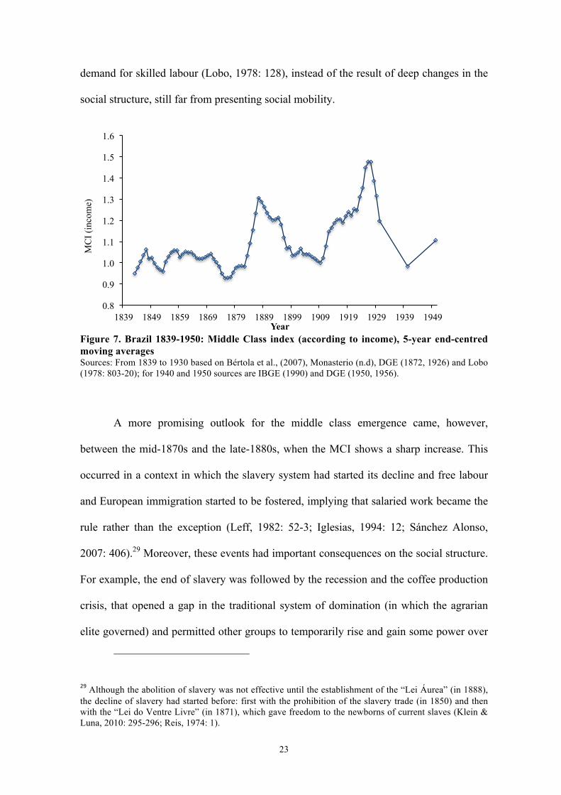
Figure 7 shows the evolution of the MCI in terms of income, which, until the late 1870s,
exhibits smooth trends, suggesting the lack of a significant middle class. This is not
surprising as there is evidence that throughout this period the recently independent
Brazilian Empire was essentially a rural economy based on slave labour. Thus, it had a
strongly hierarchical and stratified social structure, in which wage labour remained the
exception to the rule and the population of independent small farmers and slaves did not
offset the power of big landowners (Leff, 1982: 17; Mendoça, 1950: 83-4; Owensby,
1999: 15-16). Moreover, there is evidence that important structural shifts in the Brazilian
economy did not occur until the end of the nineteenth century (Leff, 1982: 166),
particularly, after the abolition of slavery and the arrival of new immigrants.28 Thus,
short-lived increases of the MCI (1843-1848; 1853-1856) might be the result of the
sparse amelioration of salaries for scarce skilled professionals in a context of increasing
28"Around 3.2 million immigrants, mainly from Southern-Europe, arrived to Brazil after the liberation of near 1 million slaves in 1888 (Goldsmith, 1986: 136)"
"
23
demand for skilled labour (Lobo, 1978: 128), instead of the result of deep changes in the
social structure, still far from presenting social mobility.
Figure 7. Brazil 1839-1950: Middle Class index (according to income), 5-year end-centred moving averages Sources: From 1839 to 1930 based on Bértola et al., (2007), Monasterio (n.d), DGE (1872, 1926) and Lobo (1978: 803-20); for 1940 and 1950 sources are IBGE (1990) and DGE (1950, 1956).
A more promising outlook for the middle class emergence came, however,
between the mid-1870s and the late-1880s, when the MCI shows a sharp increase. This
occurred in a context in which the slavery system had started its decline and free labour
and European immigration started to be fostered, implying that salaried work became the
rule rather than the exception (Leff, 1982: 52-3; Iglesias, 1994: 12; Sánchez Alonso,
2007: 406).29 Moreover, these events had important consequences on the social structure.
For example, the end of slavery was followed by the recession and the coffee production
crisis, that opened a gap in the traditional system of domination (in which the agrarian
elite governed) and permitted other groups to temporarily rise and gain some power over
29"Although the abolition of slavery was not effective until the establishment of the “Lei Áurea” (in 1888), the decline of slavery had started before: first with the prohibition of the slavery trade (in 1850) and then with the “Lei do Ventre Livre” (in 1871), which gave freedom to the newborns of current slaves (Klein & Luna, 2010: 295-296; Reis, 1974: 1). "
0.8
0.9
1.0
1.1
1.2
1.3
1.4
1.5
1.6
1839 1849 1859 1869 1879 1889 1899 1909 1919 1929 1939 1949
MC
I (in
com
e)
Year
"
24
the traditional oligarchy (Lobo, 1978: 454-55; Iglesias, 1994: 27). These groups were
mainly formed by a small urban bourgeoisie linked to commerce, which emerged under
the figures of handicraft agents (involved in the commercialisation of the internal
production) or traders (whether of imports, securities or money) (Fernandes, 1978: 26).30
This recomposition of the power structure marked the beginning of modernity and
separated the stately era from a society of classes. Thus, in this period, the increase of the
MCI witnessed some structural social change, suggesting that the seeds for the middle
class emergence started to be sowed:
“At the end of the Empire of Brazil [1889], there already existed a middle class
with clean lines. The social distance between the diverse elements of our people
was definitely extinct. The jump from one class to another, from one group to
another, was a common spectacle” (Sodré, 1944: 328).
Yet, the MCI decrease during the early years of the First Republic suggests that
this middle class in terms of income was not consolidated; on the contrary, it weakened.
It fell during the Marshall government first under the administration of Deodoro da
Fonseca (1889-1891) and then of Floriano Peixoto (1891-1894). Yet, the fall became
much more profound after the election of the first civil president, Prudente de Morais, as
this meant the return of the coffee oligarchies to power (Iglesias, 1994: 30; Fausto, 1995:
442; Mota & Lopez, 2009) and the implementation of policies designed to protect the
coffee sector to the detriment of emergening industry. 31 The credit diverted to the coffee
30"Yet, according to Fernandes (1978: 201): “What many authors denominated the crisis of the oligarchy system was not a collapse […], but the beginning of a transition which inaugurated, still under the hegemony of the oligarchy, the recomposition of the power structures, from which will shape the bourgeois power and the bourgeoisie domination. "31 These traditional oligarchies linked to the agricultural sector kept power under a patronage system, in which local oligarchs (coronéis) gave favors in return for votes. Under this period (1891-1930), known as coronelismo, “contested presidential elections were the exception; landowners had a free hand in their constituencies through control of the police and the judicial system; they rigged election as required, local political leaders automatically supported official candidates. A pact among provincial governors
"
25
sector and the deflationary policies benefiting imports and a shrinking internal market
negatively affected industry, as well as employment and wages in the secondary sector
(Lobo, et al., 1971: 249; Lobo, 1978: 487; Dean, 1992: 338-39). Therefore, the crisis of
industry together with the general lack of financing (with the exception of the coffee
sector) might have frustrated the expectations of improvement of those susceptible to
become middle class in terms of income. For example, by 1908 in Rio de Janeiro salaries
of weavers were reduced from 1$300-2$000 per day to 600-1$000, while housing rents
ranged from 8$000 to 30$000, representing the lower rent of 44 per cent of the minimum
salary and the higher rent of 50 per cent of the maximum salary (Lobo, et al., 1971:
256).32
However, a long run increasing trend in the MCI began in 1910 and lasted until
the 1930s, reporting a fast recovering of the middle class in terms of income. During this
period, despite the political prominence of the supporters of the export economy
(particularly, the interests of coffee growers), there were some initiatives favorable to
industry (Dean, 1992: 362). In particular, industry benefited from better access to credit,
inflation, and a favorable customs policy (which restricted the arrival of competitive
goods but allowed machinery imports), as well as the expansion of transportation
systems, innovation, and the growing population accompanied by expansion of effective
demand (Lobo, 1978: 471; Leff, 1982: 166-87; Wolfe, 1993: 7). Indeed, from this period
onwards, the interests of those in the industrial sector went hand in hand with those in the
coffee export sector (Dean, 1992: 362; Fausto, 1995: 428; Luna & Klein, 2014: 74). Leff
(1969: 479) argued that: “far from being ‘alternative’ patterns of development, as has
implemented this arrangement. It […] guaranteed the political hegemony of São Paulo [coffee producers] and Minas Gerais [ranchers], the two big states in the southeast.” (Abreu & Verner, 1997: 19). 32 1$000 stands for 1 mil-réis (official currency in Brazil until 1941).
"
26
some-times been suggested, export expansion and industrial development were
complementary and mutually supporting”. Therefore, boom exports in this period
favoured the development of industry (Leff, 1969: 479; Dean, 1992: 363; Baer, 2008:
27). During the first two decades of the twentieth century the sterling value of Brazilian
exports had been increasing at an annual trend of 4.2 per cent, meanwhile between 1924
and 1930 the rate of industrial growth was 6 per cent (Leff, 1969: 484-7).
This development of industry, in turn, had a profound impact on the social
structure with the creation of new professions (Furtado, 1965: 14; Wolfe, 1993: 6-7). It is
important to stress that the progress in the industrial sector increased the demand for
skilled workers in metalwork, clothing, shoe, and processed food industries. For instance:
“In Rio white-collar employees and professionals made up 20 to 30 percent of the half-
million strong work force in 1920. São Paulo’s white-collar sector […] neared 20 per cent
of the work force” (Owensby, 1999: 29). Moreover, the increasing urbanisation and
modernisation also fuelled new professional opportunities in the services and commerce
sector (Furtado, 1965: 18-19; Mota & Lopez, 2009: 427; Owensby, 1999: 49). For
example, in Rio de Janeiro “in 1919, only 38.4% of its active population was involved in
the real physical output, while 61.6% was engaged in the production of services” (Fausto,
1995: 438). Thus, throughout these two decades, the increasing middle class along with
increasing inequality might be associated with an early phase of development in a
Kuznetsian sense; that is, the result of a transition from the traditional sector to the
industrial one and the subsequent rise in wage differences. Importantly, in such a
scenario, increasing inequality linked to productivity differences did not impede but
rather fostered the rise of a middle class.
Yet, during this period there were also the risk of deterioration of the purchasing
power of middle and low income groups because of the fast increase in prices. Between

"
27
1914 and 1918 the cost of living tripled, affecting mainly the middle class, as its members
had wider budgets than the working class but not very different earnings (Owensby,
1999: 101-117). According to Owensby in 1920, the real wage of those at the 50th
percentile was 5.7 Cruzeiros (Cr$), while of those at the 20th and 10th were 5Cr$ and
3.8Cr$, respectively.33 However, this deterioration was not unchallenged: salaried
workers and those working in liberal professions started to associate together and to
undertake strikes and protests demanding the raising of salaries and the improvement of
labour conditions (Levine, 1998: 38; Paula & Monte-Mór, 2004: 11-2). These strikes
succeeded and general real wages slightly rose (Lobo, 1978: 507; Wolfe, 1993: 22),
experiencing on average an annual increase of 1.7 per cent between 1919 and 1929
(Goldsmith, 1986: 160). Consequently, it is not surprising that from 1920 to 1930 the
middle class in terms of income increased.
The consolidation of this new social middle, however, was completely frustrated
during the following years (1930-1950), demonstrated by the abrupt fall of the MCI. This
happened in a context of industrial expansion, modernisation and growth (Goldsmith,
1986: 143; Maddison, 1992: 26), but also in a context in which the income of the higher
class (now integrated by a new industrial bourgeoisie, but whose interests were linked to
those of the old oligarchy) was dramatically distancing itself from the rest:
“With the stimulus and protection of industry, the bourgeoisie felt safe and became
even wealthier. Not just the industrial bourgeoisie, but also the landowners, the
commercial and the financial ones. Labour legislation, rather than negatively
affecting the bourgeoisie, helped it to grow and consolidate” (Iglesias, 1994: 91-2).
33 1 Cr$ amounted to 1 mil-réis.
"
28
This was because during this period, under the Vargas’ regime (referred to as
Estado Novo), economic policies were focused on industrial expansion and social peace.
To address the first, Estado Novo’s industrial relation system protected industrialists’
efforts to maintain low wages, while industrial workers had no power to bargain for
higher wages and protect them, so they experienced a steady decline in real income
(Wolfe, 1993: 89-90). For instance, in São Paulo, between 1940 and 1945, all factory
workers experienced a decrease in their real income of around 33 per cent (Wolfe, 1993:
102, Tab.4.2). Social order, in turn, was maintained by means of repression and welfare
programs through co-opted unions which concentrated around social services (Skidmore,
1967: 40; Chacón, 1977: 56; Wolfe, 1993: 100).
Meanwhile, the heterogeneous middle class felt divided between joining worker
protests or backing the interests of powerful entrepreneurs (Fausto, 1989: 84-9),
politically abandoned and without any bargaining power (Owensby, 1999: 185-202). For
instance, in São Paulo, when there were wage increases the increase of those of skilled
workers was rather modest (about 11 per cent) in comparison to those of unskilled
workers (about 38 per cent), as industrialists counted on the authoritarian Estado Novo’s
industrial relations to bargaining power of the highly skilled (Wolfe, 1993: 102). In
addition to modest nominal wages increases, the recurrent inflation increased of the cost
of living, especially during the World War II (Goldsmith, 1986: 158, Tab.IV-7) with
dramatic consequences on the middle class’ real income.
Therefore, during this period, increasing inequality might be explained in terms of
the Lewis (1954) model, in which the elastic supply of labour (in a context of population
growth and internal migration) facilitated the capital sector to keep low wages. Crucially,
in such a context, despite the industrialization process, the continued increase of
inequality had devastating consequences for the middle class.
"
29
6. Brazil (1839-1950): Middle class evolution in terms of status
Although the income dimension is important to define the middle class, as mentioned in
Section 3, there are other subjective dimensions that characterised the middle class. In
particular, in Brazil during the nineteenth and twentieth centuries, status and appearance
identified people with a particular social group more than their income did. Noteworthy,
one of the main elements that conformed people to a particular class or status was their
profession. 34 “Class was a such powerful determinant of position that the attributes of
class would often influence the definition of color [...] Black lawyers were often defined
as mulattoes, just as mulattoes ones were defined as white” (Klein & Luna, 2010: 268).
Indeed, the middle class was so concerned about keeping its status, that they might prefer
a low paid non-manual job than any better remunerated work in the manual sector: “[it]
was likely less a conscious effort by middle-class people to imitate the rich than an
imperative not to be confused with the working-class poor” (Owensby, 1999: 106).
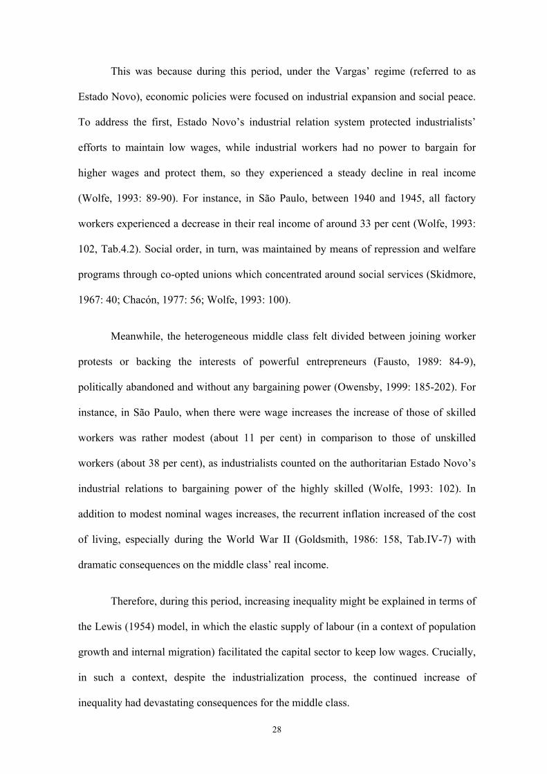
Therefore, Figure 8 shows the MCI performance in terms of status linked to the
professional category.
34 Other characteristic elements of the Brazilian middle class, at that time, were expenditures on: clothing, servants, culture and education. (Owensby 1999:107-10).
"
30
Figure 8. Brazil 1839-1950: Middle Class index (according to status) 5- year moving averages. Sources: From 1839 to 1930 based on Bértola et al., (2007), Monasterio (n.d), DGE (1872, 1926) and Lobo (1978: 803-20); for 1940 and 1950 sources are IBGE (1990) and DGE (1950, 1956). It suggests that the emergence of the middle class in terms of status remained
unfeasible until the early twentieth century, as the MCI remained stagnant or declining
until then. The exception took place between the 1850s and mid-1860s, when we observe
a brief increase. This increase might have been linked to the expansion of manufacturing
activity and the temporal rise in the demand of skilled labour. For instance, there is
evidence that on the eve of the Paraguayan War there was increasing demand in skilled
carpenters for the construction of fleets (Lobo et al., 1973: 156). Meanwhile during those
years there was increasing investment in new industrial undertakings, shipping and urban
transport companies (Jaguaribe, 1968: 133). In this vein, according to Sodré (1939: 71)
there is evidence that after the prohibition of slave trade in 1850 public works contracts
required the exclusion of slaves, exemplified by the works of the Union and Industry
Highway, which mostly hired German and Portuguese workers.35 Notably, since the rise
35"The Union and Industry Highway (Estrada de Rodagem União e Indústria) was the road that connected the cities of Petrópolis and Juiz de Fora in the South-East of Brazil."
1
2
3
4
5
6
7
1839 1849 1859 1869 1879 1889 1899 1909 1919 1929 1939 1949
MC
I (st
atus
)
Year
"
31
of the MCI in terms of status seems due to a temporal rise in the demand for skilled
professionals, this did not mean any transformation of the social structure.
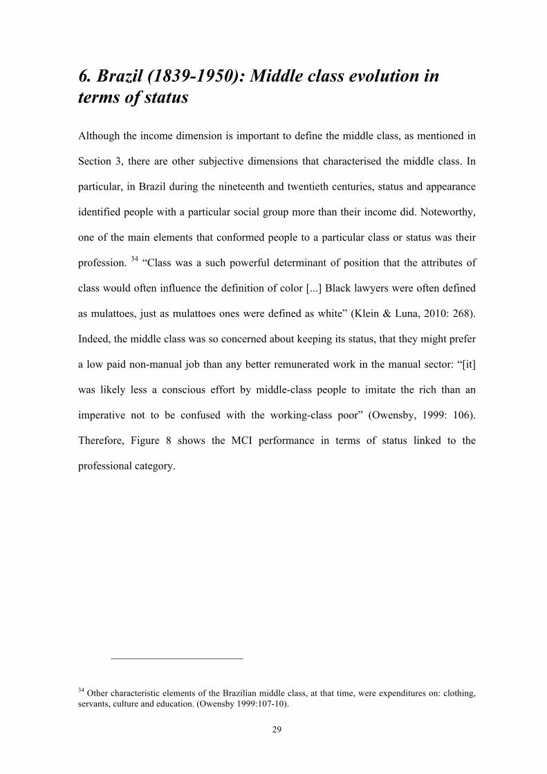
Indeed, in Figure 9 can be observed that the increase in the middle class in terms of
income during the nineteenth century went along with the immobility of the middle class
in terms of status. This suggests that temporal increases in mean income were not
translated into real upwards movements in the social scale, denoting a highly stratified
society.
Figure 9. Brazil 1839-1950: Middle Class index (according to status and income) 5- year moving averages. Sources: From 1839 to 1930 based on Bértola et al., (2007), Monasterio (n.d), DGE (1872, 1926) and Lobo (1978: 803-20); for 1940 and 1950 sources are IBGE (1990) and DGE (1950, 1956).
Nevertheless, from the early 1910s, in a context of increasing modernisation and
urbanisation, as happened in terms of income, the middle class in terms of status grew
vigorously until the 1930s. During those years, once the work force seems to have been
industrialized, industry, non-manual sectors expanded and the demand for professional
qualifications and higher education grew in direct proportion to the expansion of these
non-manual sectors (Owensby, 1999: 29-30), so did the number of people employed in
0.8
0.9
1.0
1.1
1.2
1.3
1.4
1.5
1.6
1.0
2.0
3.0
4.0
5.0
6.0
7.0
1839 1849 1859 1869 1879 1889 1899 1909 1919 1929 1939 1949 M
CI (
inco
me)
MC
I (st
atus
)
Year Middle Class (status) Middle Class (income)
"
32
liberal professions, administration officer’s corps and commerce (Furtado, 1965: 15;
Owensby, 1999: 28). Indeed, according to Owensby (1999: 29) this process “had the
effect of putting greater social distance between respectable employees and deskilled
laborers”. In this sense, those who felt part of the middle class in terms of status (for
example, white-collar salary earners, commercial employees and clerks) became the most
vulnerable to economic crisis and inflation, as they had to struggle to keep up
appearances with wider budgets, when prices of clothing and rent (typically demanded by
middle class consumers) increased more than, for example, food prices (Goldsmith 1986:
160).
Moreover, the prestige of having a non-manual profession acted as an incentive to
choose, if possible, those jobs of higher status even though they were worse paid. Indeed,
some manual work was better remunerated than non-manual work, but the middle class
preferred to perform non-manual activities (Owensby, 1999: 54). This implies that,
contrary to what happened in the nineteenth century, when the increased middle class in
terms of income did not lead to a middle class emergence in terms of status, during the
early twentieth century, the rise of the middle class in terms of status became more
evident than it did in terms of income. Probably, for the same reason the decline of the
middle class in terms of status took place later and to a lesser degree than in terms of
income.
Yet the fall of the MCI, between 1930 and 1950, also shows evidence of the
damage of the middle class during the Vargas era in terms of status. Under the Estado
Novo, the government handed out favours to interest groups while giving prerogatives to
industrial workers (such as minimum wages, eight-hour day, holidays with pay, job
security and a social security system) with a view to maintain populist support from
labour groups (Maddison 1992: 21). Meanwhile, those in the middle were dropped by the
"
33
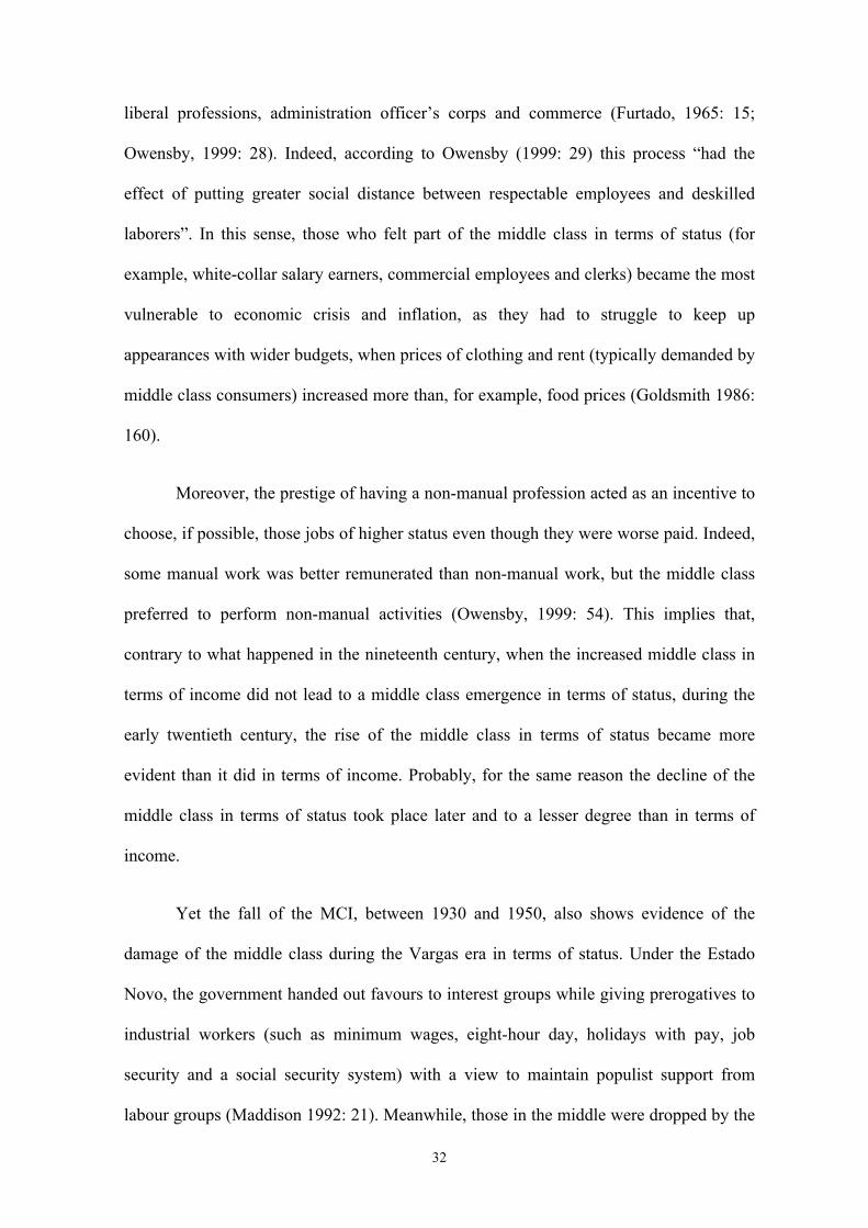
wayside, getting weaker and struggling to keep their social status, which, apparently most
of them lost. According to my estimations the middle class in terms of status passed from
being 26 per cent of the active population in 1930 to 16 per cent in 1950, meanwhile
those in the lower class increased from 73 per cent to 82 per cent over the same period. It
is worth noting that this weakening of the middle class occurred in a context of
modernisation and economic growth, however, accompanied by increasing inequality,
social repression and populist policies. Consequently, the middle class’ prospects for
consolidation became unfeasible.
In sum, we cannot ignore that substantial social structural change occurred in
Brazil over the period under review. The decline of slavery (starting in the 1850s), the
reduction of inequality (during the late nineteenth century), and the process of
modernisation and urbanisation (from the early twentieth century) seems to have been
crucial for the emergence of the middle class. However, from the 1930s the continuous
increase in inequality, along with a low social cohesion, could have impeded the
consolidation of a middle class. On the one hand, social issues were considered by
governments as dangers that needed be repressed; on the other hand, the urban population
did not yet have the self-awareness or class consciousness necessary to give coherence to
its complaints (Furtado, 1965: 19). This, in turn, might have facilitated the emergence of
a populist government, which focused on the elite’s interests and satisfied immediate
population aspirations with welfare programs, but which did not pay too much attention
to the medium stratums. Consequently, during the following years, until 1950, the
consolidation of the middle class appears to have been frustrated
"
34
7. Concluding remarks
As in the most recent decades, Brazil experienced episodes of rapid economic growth
between the mid-nineteenth and mid-twentieth centuries (recording periods of per head
GDP growth of 2 and 3 per cent annually). However, unlike recent times, there is little
evidence on the rise of the middle class during that period and its connection with
inequality.
After highlighting the inconsistency of nineteenth century Gini estimates and the
underlying ambiguity on the timing of the emergence of the middle class, this article
explored Brazil’s income distribution between 1839 and 1950 from two perspectives:
inequality and polarisation. The article showed that Brazil exhibited low inequality from
1839 until 1913, probably due to low income levels, which impeded the emergence of the
middle class. Then inequality started to grow from 1913 onwards, apparently linked to an
early phase of economic growth in a Kuznetsian sense, in which the middle class arose.
However, between 1930 and 1950 the increase in inequality might be explained in terms
of the Lewis (1954) elasticities model, in which the elastic supply of labour in a context
of growing population maintained wages at subsistence level blocking the consolidation
of the middle class.
In the light of these results, the MCI shows that the seeds for the efflorescence of
the middle class were sowed in the late nineteenth century when the decline of the slave
system led to a more competitive social order. Yet, its emergence, in terms of both
income and status, should be placed during the three first decades of the twentieth
century, in a context of expansion of industry and modernisation. Interestingly, from the
1930 until the end of the Vargas era, still in a context of urbanisation and growth,
increasing inequality and social repression led the middle class to shrink, both in terms of
"
35
income and status. Importantly, results suggesting that persistent inequality, despite
economic growth, blocks the consolidation of the middle class and the eradication of
poverty, might entail relevant social policy implications for Brazil nowadays and other
emerging middle income countries. Yet, broad conclusions would require further
investigation on the connection between growth, inequality and the consolidation of the
middle class at both country and cross-national levels.
References
Abreu, M. D., & Verner, D. (1997). Long term Brazilian economic growth:1930-94.
París: OECD, Development Center Studies.
Acemoglu, D., Johnson, S., & Robinson, J. (2002). Reversal of Fortune: Geography and
Institutions in the Making of the Modern World Income Distribution. Quarterly
Journal of Economics, 117(4), 1231-94.
Affonseca, L. (1920). O custo da vida na cidada do Rio de Janeiro. Rio de Janeiro.
Baer, W. (2008). The Brazilian Economy: Growth and Development (6th ed.). London:
Lynne Rienner Publishers.
Banerjee, A., & Duflo, E. (2008). What is Middle Class about the Middle Classes around
the World? Journal of Economic Perspectives, 22(2), 3-28.
Bértola, L., Castelnovo, C., Reis, E., & Willebald, H. (2007). Exploring the distribution
of income in Brazil, 1839-1939. Primer Congreso Latinoamericano de Historia
Económica (CLADHE I), Montevideo.
"
36
Bértola, L., Castelnovo, C., Reis, E., & Willebald, H. (2012). Income Distribution in
Brazil in 1870-1920. XVII Jornadas Anuales de Economía, Banco Central del
Uruguay, Montevideo.
Birdsall, N. (2010). The (indispensable) Middle Class in Developing Countries. In R.
Kanbur , & M. Spence (Eds.), Equity and Growth in a Globalizing World (pp.
157-87). Washington, D.C.: Commission on Growth and Development.
Birdsall, N., & Londoño, J. (1997). Asset Inequality Matters: Lessons from Latin
America. IDB Working Paper Series 284, Washington, D.C.: Inter-American
Development Bank.
Bourguignon, F. (2000). The Pace of Economic Growth and Poverty Reduction (mimeo
ed.). (W. Bank, Ed.) París: Delta.
Chacón, V. (1977). Estado e Povo no Brasil: As Experiências do Estado Novo e da
Democracia Populista: 1937-1964. Rio de Janeiro: José Olympo.
Côrtes Neri, M. (2010). A Nova Classe Média. O Lado Brilhante dos Pobres. Rio de
Janeiro: Fundação Getulio Vargas.
Cruces, G., López-Calva, L., & Battistón, D. (2011). Down and Out or Up and In?
Polarisation Based Measures of the Middle Class for Latin America. CEDLAS
Working paper 113, La Plata: Universidad Nacional de la Plata.
Dean, W. (1992). La economía brasileña, 1870-1930. In L. Bethell (Ed.), Historia de
América Latina (Vol. 10, pp. 333-69). Barcelona: Editiorial Crítica.
DGE-Diretoria Geral de Estatística. (1872). Recensamento Geral do Brazil 1872. Rio de
Janeiro: Typhografía da Estatística.
"
37
DGE-Diretoria Geral de Estatística. (1895). Recensamento Geral de La República dos
Estados Unidos do Brazil em 1890. Rio de Janeiro: Typhografía da Estatística.
DGE-Diretoria Geral de Estatística. (1926). Recensamento Geral do Brazil 1920. Rio de
Janeiro: Typhografía da Estatística.
DGE-Diretoria Geral de Estatística. (1950). Recensamento Geral do Brazil 1940. Rio de
Janeiro: Typhografía da Estatística.
DGE-Diretoria Geral de Estatística. (1956). Recensamento Geral do Brazil 1950. Rio de
Janeiro: Typhografía da Estatística.
Easterly, W. (2001). The middle class consensus and economic development. Journal of
Economic Growth, 6(4), 317-35.
Engerman, S., & Sokoloff, K. (1997). Factor Endowments, Institutions, and Differential
Paths of Growth Among New World Economies: A View From Economic
Historians of the United States. In S. Haber (Ed.), How Latin America Fell Behind
(pp. 260-304). Stanford: Stanford University Press.
Esteban, J. (1996). Desigualdad y polarización. Una aplicación a la distribución
interprovincial de la renta en España. Revista de Economía Aplicada, 4(11), 5-26.
Esteban, J., & Ray, D. (1994). On the measurement of polarization. Econometrica, 62(4),
819-51.
Esteban, J., Gradín, C., & Ray, D. (2007). An extensions of a measure of polarization,
with an application to the income distribution of five OECD countries. Journal of
Economic Inequality, 5(1), 1-19.
"
38
Fausto, B. (1989). Society and Politics. In L. Bethell (Ed.), Brazil Empire and Republic,
1822-1930 (pp. 257-307). Cambridge: Cambridge University Press.
Fausto, B. (1995). Brasil: estructura social y política de la primera república, 1889-1930.
In L. Bethell (Ed.), Historia de América Latina (Vol. 10, pp. 414-55). Barcelona:
Editorial Crítica.
Fernandes, F. (1978). La revolución burguesa en Brasil. México: Siglo XXI.
Ferreira, F. (2000). Os determinantes da desigualdade de renda no Brasil: Luta de
classes ou heterogeneidad educacional? (E. Henriques, Ed.) Rio de Janeiro:
Pontificia Universidade Católica de Rio de Janeiro, Departamento de Economía.
Ferreira, F., Messina, J., Rigolini, J., López Calva, L., Lugo, M., & Vakis, R. (2013).
Economic Mobility and the Rise of the Latin American Middle Class. Washington,
D.C.: The World Bank.
Foster, J., & Wolfson, M. (2010). Polarization and the Decline of the Middle Class:
Canada and the US. The Journal of Economic Inequality, 8(2), 247-73.
Furtado, C. (1965). La dialéctica del desarrollo: diagnóstico de la crisis del Brasil.
México: Fondo de Cultura Económica.
Goldsmith, R. (1986). Brasil 1850-1984: Desenvolvimento Financieiro sob um Século de
Inflação. Rio de Janeiro: Banco Bamerindus do Brasil.
Gradín, C. (2000). Polarization by Sub-populations in Spain, 1973-91. Review of Income
and Wealth, 46(4), 457-74.
"
39
Gradín, C., & del Río, C. (2001). Desigualdad, Polarización y Pobreza en la Distribución
de la renta en Galicia. Monografía 11, A Coruña: Instituto de Estudios
Economicos de Galicia-Pedro Barrié de la Maza.
IBGE-Instituto Brasileiro de Geografía e Estatística. (1990). Estatísticas Históricas do
Brasil. Series Econômicas, Demográficas e Sociais 1550 a 1988 (2 ed. rev. e atual
do v.3 de Séries estatísticas retrospectivas ed., Vol. 3). RÍo de Janeiro.
IBGE-Instituto Brasileiro de Geografía e Estatística. (2007). Estatísticas do Século XX.
Rio de Janeiro: IBGE, Centro de Documentaçao e Disseminação de Informações.
IBGE-Instituto Brasileiro de Geografía e Estatística. (marzo 2011). Comunicación Social:
Cuentas Nacionales Trimestrales.
Iglesias, F. (1994). Breve historia contemporánea del Brasil. México: Fondo de Cultura
Económica.
Jaguaribe, H. (1968). Economic & Political Development: A theoretical approach & A
Brazilian Case Study. Cambridge, Mass: Harvard University Press.
Klein, H. S. (1986). African Slavery in Latin America and the Caribbean. New York:
Oxford University Press.
Klein, H. S. (1995). A participação política no Brasil do século XIX: os votantes de São
Paulo em 1880. Dados- Revista de Ciências Sociais, 38(3), 527-544.
Klein, H. S., & Luna, F. V. (2010). Slavery in Brazil. New York: Cambridge University
Press.
"
40
Kuznets, S. (1955). Economic Growth and Income Inequality. The American Economic
Review, 45(1), 1-28.
Leff, N. (1969). Long-Term Brazilian Economic Development. The Journal of Economic
History, 29(3), 473-93.
Leff, N. (1982). Underdevelopment and Development in Brazil. Vol.I: Economic
Structure and Change, 1822-1947. London: George Allen & Unwin.
Levine, R. (1998). Father of the poor? Vargas and his era. Cambridge: Cambridge
University Press.
Lewis, W. (1954). Economic Development with Unlimited Supplies of Labour. The
Manchester School of Economic and Social Studies, 22(2), 139-91.
Loayza, N., Rigolini, J., & Llorente, G. (2012). Do Middle Classes Bring Institutional
Reforms? Policy Research Working Paper 6015, Washington D.C.: The World
Bank.
Lobo, E. (1978). Historia do Rio de Janeiro: do capital comercial ao capital industrial e
financeiro. Rio de Janeiro: Instituto Brasileiro de Mercado de Capitais.
Lobo, E., Canavarros, O., Feres, Z., Gonçalves, S., & Barbosa Madureira, L. (1971).
Evolução dos preços e do padrão de vida no Rio de Janeiro 1820-1930. Revista
Brasileira de Economía, 25(4), 235-66.
Lobo, E., Canavarros, O., Feres, Z., Novais, S., & Barbosa Madureira, L. (1973). Estudo
das categorias socioprofissionais, dos salários e do custo da alimentação no Rio de
Janeiro de 1820 a 1930. Revista Brasileira de Economía, 27(4), 129-76.
"
41
López-Calva, L., & Ortiz-Juárez, E. (2011). A vulnerability approach to the definition of
the middle class. Policy Research Working Paper 5902, Washington, D.C.: The
World Bank.
Lora, E., & Fajardo, J. (2011). Latin American Middle Classes; The distance between
perception and reality. Working Paper 275, Washington, D.C.: Inter-American
Development Bank.
Luna, F. V., & Klein, H. S. (2014). The Economic and Social History of Brazil since
1889. New York: Cambridge University Press.
Maddison, A. (1992). The Political Economy of Poverty, Equity and Growth: Brazil and
Mexico. New York: Oxford University Press.
Maddison, A. (1995). Monitoring the World Economy, 1820-1992. Paris: OECD.
Maddison, A. (2003). The World Economy: Historical Statistics. París: OECD .
Mendoça, R. (1950). Breve Historia del Brasil. Madrid: Ediciones Cultura Hispánica.
Milanovic, B. (2006). An estimate of average income and inequality in Byzantium around
year 1000. Review of Income and Wealth, 52(3), 449-70.
Milanovic, B. (2009). Preindustrial inequality. In S. Durlauf, & L. Blume (Eds.), The
New Palgrave Dictionary of Economics (Online Edition ed.). Palgrave
Macmillan.
Milanovic, B. (2011). A short history of global inequality: the past two centuries.
Explorations in Economic History, 48, 494-506.
"
42
Milanovic, B., Lindert, P. H., & Williamson, J. G. (2010). Pre-industrial Inequality. The
Economic Journal, 121(551), 255–72.
Milanovic, B., Lindert, P., & Williamson, J. (2007). Measuring Ancient Inequality".
NBER Working Paper 13550, Cambridge, Mass: National Bureau of Economic
Research.
Monasterio, L. (2010). Brazilian spatial dynamics in the long term (1872-2000) "path
dependency" or "reversal of fortune"? Journal of Geographical Systems, 12 (1),
51-67.
Mota, C., & Lopez, A. (2009). Historia de Brasil: una interpretación. Salamanca:
Ediciones Universidad de Salamanca.
Nunes, N. (2003). A experiência eleitoral em Campos dos Goytacazes (1870-1889):
Freqüência eleitoral e perfil da popilação votante. Dados- Revista de Ciências
Sociais, 46(2), 311-43.
Onody, O. (1960). A inflação brasiliera, 1820-1958. Rio de Janeiro: Vervuert Verlag.
Owensby, P. (1999). Intimate Ironies. Modernity and the Making of a Middle-Class Lives
in Brazil. Stanford, California: Stanford University Press.
Paula, J., & Monte-Mór, R. (2004). Formação Histórica: Três Momentos da História de
Belo Horizonte. Belo Horizonte: CEDEPLAR FACE/UFMG.
Prados de la Escosura, L. (2007a). Inequality and Poverty in Latin America: A Long-Run
Exploration. In T. Hatton, K. O'Rourke, & A. M. Taylor (Eds.), The New
Comparative Economic History (pp. 291-315). Cambridge, Mass: MIT press.
"
43
Prados de la Escosura, L. (2007b). International Inequality and Polarisation in Living
Standards, 1870-2000: Evidence from the Western World. Working Papers in
Economic History 07-05, Madrid: Universidad Carlos III de Madrid.
Ravallion, M. (2001). Growth, Inequality and Poverty: Looking Beyond Averages. World
Development, 11(29), 1803-15.
Ravallion, M. (2010). The developing world's bulging (but vulnerable) middle class.
World Development, 38(4), 445-54.
Ray, D. (1998). Development Economics. Princeton: Princeton University Press.
Reis, J. (1974). Abolition and the economics of slaveholding in north east Brazil. Institute
of Latin American Studies Occasional Papers 11, Glasgow: University of
Glasgow.
SAE- Secretaría de Assuntos Estratégicos. (2012). Vozes da Classe Media. Retrieved
from http://www.sae.gov.br
Sánchez Alonso, B. (2007). The Other Europeans: Immigration into Latin American and
the International Labour Market (1870-1930). Journal of Iberian and Latin
American Economic History(3), 395-426.
Skidmore, T. E. (1967). Politics in Brazil 1930-1964: An experiment in democracy. New
York: Oxford University Press.
Sodré, N. (1944). Formação da sociedad brasileira. São Paulo: José Olympio.
Solimano, A. (2008). The Middle Class and the Development Process. Serie
Macroeconomía del Desarrollo 65, Santiago de Chile: United Nations-ECLAC.
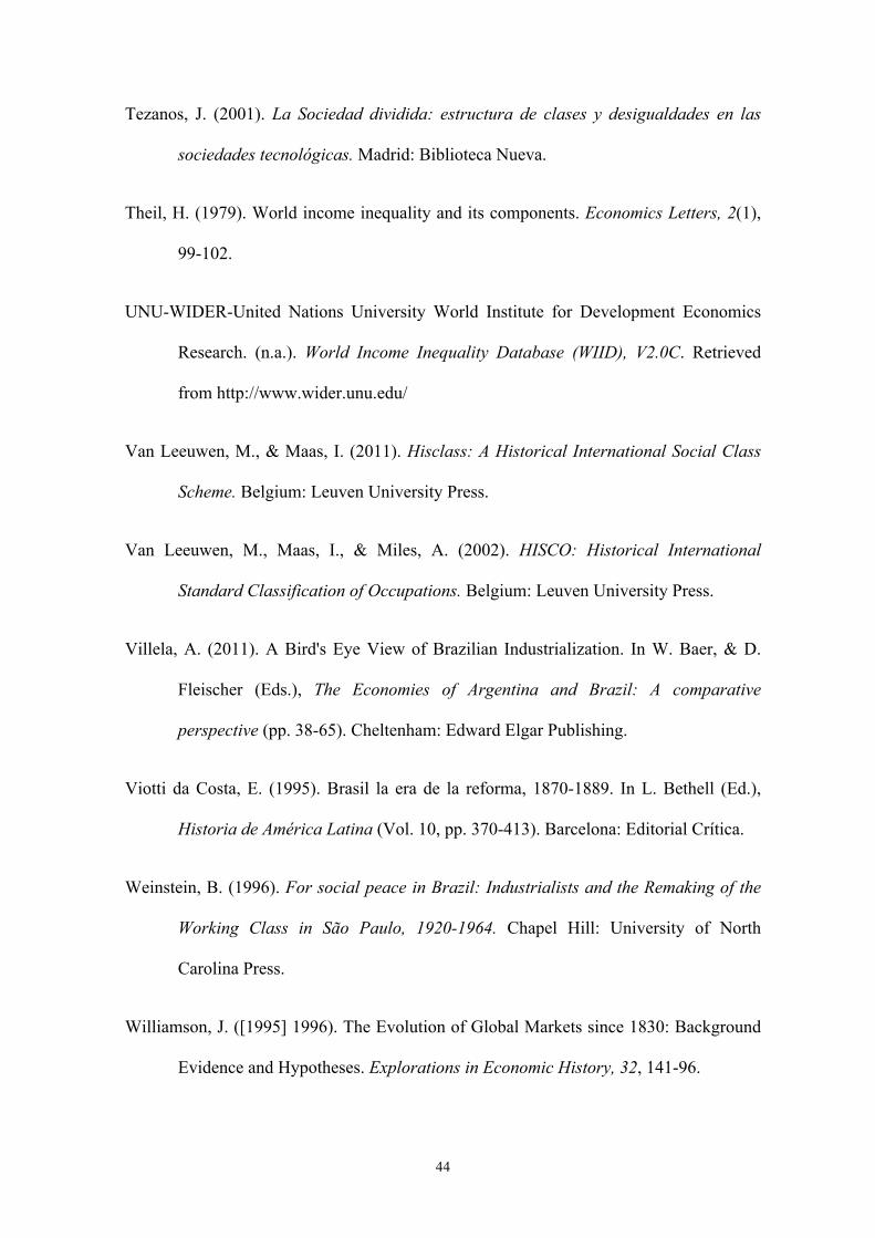
"
44
Tezanos, J. (2001). La Sociedad dividida: estructura de clases y desigualdades en las
sociedades tecnológicas. Madrid: Biblioteca Nueva.
Theil, H. (1979). World income inequality and its components. Economics Letters, 2(1),
99-102.
UNU-WIDER-United Nations University World Institute for Development Economics
Research. (n.a.). World Income Inequality Database (WIID), V2.0C. Retrieved
from http://www.wider.unu.edu/
Van Leeuwen, M., & Maas, I. (2011). Hisclass: A Historical International Social Class
Scheme. Belgium: Leuven University Press.
Van Leeuwen, M., Maas, I., & Miles, A. (2002). HISCO: Historical International
Standard Classification of Occupations. Belgium: Leuven University Press.
Villela, A. (2011). A Bird's Eye View of Brazilian Industrialization. In W. Baer, & D.
Fleischer (Eds.), The Economies of Argentina and Brazil: A comparative
perspective (pp. 38-65). Cheltenham: Edward Elgar Publishing.
Viotti da Costa, E. (1995). Brasil la era de la reforma, 1870-1889. In L. Bethell (Ed.),
Historia de América Latina (Vol. 10, pp. 370-413). Barcelona: Editorial Crítica.
Weinstein, B. (1996). For social peace in Brazil: Industrialists and the Remaking of the
Working Class in São Paulo, 1920-1964. Chapel Hill: University of North
Carolina Press.
Williamson, J. ([1995] 1996). The Evolution of Global Markets since 1830: Background
Evidence and Hypotheses. Explorations in Economic History, 32, 141-96.
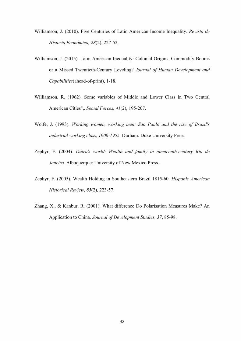
"
45
Williamson, J. (2010). Five Centuries of Latin American Income Inequality. Revista de
Historia Económica, 28(2), 227-52.
Williamson, J. (2015). Latin American Inequality: Colonial Origins, Commodity Booms
or a Missed Twentieth-Century Leveling? Journal of Human Development and
Capabilities(ahead-of-print), 1-18.
Williamson, R. (1962). Some variables of Middle and Lower Class in Two Central
American Cities",. Social Forces, 41(2), 195-207.
Wolfe, J. (1993). Working women, working men: São Paulo and the rise of Brazil's
industrial working class, 1900-1955. Durham: Duke University Press.
Zephyr, F. (2004). Dutra's world: Wealth and family in nineteenth-century Rio de
Janeiro. Albuquerque: University of New Mexico Press.
Zephyr, F. (2005). Wealth Holding in Southeastern Brazil 1815-60. Hispanic American
Historical Review, 85(2), 223-57.
Zhang, X., & Kanbur, R. (2001). What difference Do Polarisation Measures Make? An
Application to China. Journal of Development Studies, 37, 85-98.
"
46
Appendix
Table 1. HISCLASS classification and group aggregation.
Sources: Based on the classification table in van Leeuwen, M. and I. Maas (2011)
Class number Class label Skill levelManual/ Non
manual 3 Groups
aggregation 2 Groups
aggregation
1 Higher managers HIGH HIGH CLASS2 Higher profesionals [1, 2] [1, 2 ] HIGH CLASS
NON MANUAL [1, 2, 3, 4, 5]3 Lower managers MEDIUM [1, 2, 3, 4, 5]4 Lower proffesionals and clerical and sales personel [3, 4]
MIDDLE CLASS5 Lower clerical and sales personel LOW [3, 4, 5, 6, 7]
[5]6 Foremen7 Medium skilled workers MEDIUM8 Farmers and fishermen [6, 7, 8] LOW CLASS
[6, 7, 8, 9, 10, 11, 12]9 Lower skilled workers LOW MANUAL LOW CLASS
10 Lower skilled farm workers [9, 10] [6, 7, 8, 9, 10, 11, 12,] [ 8, 9, 10, 11, 12]
11 Unskilled workers UNSKILLED12 Unskilled farm workers [11, 12]
"
47
Table 2. Brazil 1839-1898: sources and data
Notes: English translations of professions are based on HISCO database. * Bértola’s et al.,(2007) estimations are mostly based on Lobo (1978). ** Lobo’s estimations have been adjusted according to those reported by other authors for specific periods: Klein (1995) provides data for 1880; Nunes (2003) from 1870 to 1889; Monasterio for 1880 and 1881; and chosen Lobo’s sample for adjustment is from 1879 to 1881. *** Equivalences are based on information of industrial salaries from IBGE (1990).
POPULATION DATA INCOME'DATA Profession classification acording to 1872 census Estimations:Artistas (artist)Advogados (lawyer)Canteiros, Calceteiros e Mineiros (stone cutter, platelayer, miner)Capitalistas e Proprietários (landowner, proprietary)
Cirurgiões (doctor surgeon)
Costureiras (dressmaker) Based on Lobo (1978), Bértola, L. et al. (2007) and Monasterio (n.d.)*
Criados e Jornaleiros (house servant and journeyman)Escravos (slave)Juízes (judge)
Oficiais de Justiça (judicial solicitor)
Op. Em Edificações (construction worker)
Op. Em Metais (blacksmith)Procuradores (procurator)Serviço Doméstico (domestic servant)
Sem Profissão (without any profession)
Capelão (priest)
Administraçao pública (Government administrators)Comerciantes, Guarda-Livros e Caixeiros (retailer, book-keeper, cashier)Enfermeiros (nurse)Farmacêuticos (chemist) Based on Lobo (1978)**Lavradores (farmer)Médicos (doctor)
Operários em Madeiras (wood treaters)
Professores e Homens de Letras (teacher and first letters teacher)Sacristão (sexton)
Criadores (stock-breeder) Equal to horticulturit's wage in Lobo (1978)***Notários e Escrivães (notary) Equal to lawyer's wage Op. De Calçado (shoemaker) Equal to 89% carpenter's wage in Lobo (1978)***Op. De Chapéus (hat maker) Equal to 89% carpenter's wage in Lobo (1978)***Op. De Vestuários (dressmaker) Equal to 89% carpenter's wage in Lobo (1978)***Op. Em Couros e Peles (leather goods maker) Estimated as 87% carpenter's wage in Lobo (1978)***Op. Em tecidos (weaver) Estimated as 60% carpenter's wage in Lobo (1978)***Op. Em Tinturaria (dyer worker) Equal to carpenter's wage in Lobo (1978)***Parteiros (midwife) Equal to nurse's wage in Lobo (1978)
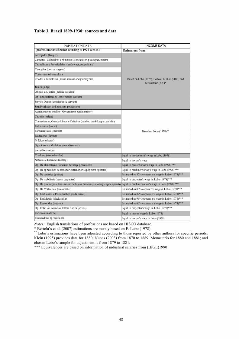
"
48
Table 3. Brazil 1899-1930: sources and data
Notes: English translations of professions are based on HISCO database. * Bértola’s et al.,(2007) estimations are mostly based on E. Lobo (1978). ** Lobo’s estimations have been adjusted according to those reported by other authors for specific periods: Klein (1995) provides data for 1880; Nunes (2003) from 1870 to 1889; Monasterio for 1880 and 1881; and chosen Lobo’s sample for adjustment is from 1879 to 1881. *** Equivalences are based on information of industrial salaries from (IBGE)1990
POPULATION DATA INCOME'DATA (profession classification acording to 1920 census) Estimations from:Advogados (lawyer)Canteiros, Calceteiros e Mineiros (stone cutter, platelayer, miner)Capitalistas e Proprietários (landowner, proprietary)
Cirurgiões (doctor surgeon)
Costureiras (dressmaker)Criados e Jornaleiros (house servant and journeyman) Based on Lobo (1978), Bértola, L. et al. (2007) and
Monasterio (n.d.)*Juízes (judge)
Oficiais de Justiça (judicial solicitor)
Op. Em Edificações (construction worker)
Serviço Doméstico (domestic servant)
Sem Profissão (without any profession)
Administraçao pública ( Government administrator)
Capelão (priest)
Comerciantes, Guarda-Livros e Caixeiros (retailer, book-keeper, cashier)Enfermeiros (nurse)Farmacêuticos (chemist) Based on Lobo (1978)**Lavradores (farmer)Médicos (doctor)
Operários em Madeiras (wood treaters)
Sacristão (sexton)
Criadores (stock-breeder) Equal to horticulturit's wage in Lobo (1978)Notários e Escrivães (notary) Equal to lawyer's wage Op. De alimentação (food and beverage processors) Equal to press worker's wage in Lobo (1978)***
Op. De apparelhos de transporte (transport equipment operator) Equal to machine worker's wage in Lobo (1978)***Op. De cerámica (potter) Estimated as 87% carpernter's wage in Lobo (1978)***
Op. De mobiliario (bench carpenter) Equal to carpenter's wage in Lobo (1978)***Op. De producçao e transmissao de forças fhisicas (stationary engine operator)Equal to machine worker's wage in Lobo (1978)***
Op. De Vestuários (dressmaker) Estimated as 89% carpenter's wage in Lobo (1978)***
Op. Em Couros e Peles (leather goods maker) Estimated as 87% carpernter's wage in Lobo (1978)***Op. Em Metais (blacksmith) Estimated as 96% carpernter's wage in Lobo (1978)***Op. Em tecidos (weaver) Estimated as 60% carpernter's wage in Lobo (1978)***Op. Relat. Ás sciencias, lettras e artes (artists) Equal to carpenter's wage in Lobo (1978)***
Parteiros (midwife) Equal to nurse's wage in Lobo (1978)Procuradores (procurator) Equal to lawyer's wage in Lobo (1978)
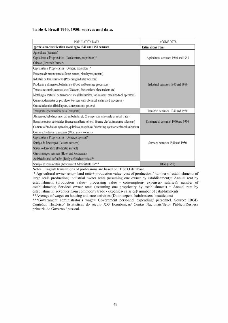
"
49
Table 4. Brazil 1940, 1950: sources and data.
Notes: English translations of professions are based on HISCO database. * Agricultural owner rents= land rents+ production value- cost of production / number of establishments of large scale production; Industrial owner rents (assuming one owner by establishment)= Annual rent by establishment (production value+ processing value - consumption- expenses- salaries)/ number of establishments; Services owner rents (assuming one proprietary by establishment) = Annual rent by establishment (revenues from commodity trade - expenses- salaries)/ number of establishments. **Average of wages on housing and care activities (Doorkeepers, hairdressers, beauticians) ***Government administrator’s wage= Government personnel expending/ personnel. Source: IBGE/ Conteúdo Histórico/ Estatísticas do século XX/ Econômicas/ Contas Nacionais/Setor Público/Despesa primaria do Governo / pessoal.
POPULATION DATA INCOME'DATA (profession classification acording to 1940 and 1950 censuses Estimations from:Agricultura (Farmers)Capitalistas e Proprietários (Landowners, proprietors)* Agricultural censuses 1940 and 1950Criaçao (Livetock Farmer)Capitalistas e Proprietários (Owners, propietors)*Extacçao de mat.mineraes (Stone cutters, platelayers, miners)Industria de transformaçao (Procesing industry workers)Produçao e alimentos, bebidas, etc (Food and beverage processors) Industrial censuses 1940 and 1950Texteis, vestuario,caçados, etc (Weavers, dressmakers, shoe makers etc)Metalurgia, material de transporte, etc (Blacksmiths, toolmakers, machine-tool operators)Química, derivados de petroleo (Workers with chemical and related processes ) Outras industrias (Bricklayers, stonemansons, potters)Transportes y comunicaçoes (Transports) Transport censuses 1940 and 1950Alimentos, bebidas, comercio ambulante, etc (Salesperson, wholesale or retail trade)Bancos e outras actividades financeiras (Bank tellers, finance clerks, insurance salesman) Commercial censuses 1940 and 1950Comercio Productos agrícolas, quimicos, maquinas (Purchasing agent or technical salesman)Outras actividades comerciais (Other sales workers)Capitalistas e Proprietários (Owner, propietor)*Serviço de Recreaçao (Leisure services) Services censuses 1940 and 1950Servicio doméstico (Domestic servant)Otros serviços pessoais (Hotel and Restaurant)Actividades mal definidas (Badly defined activities)**Serviço governamentais (Government Administrators)*** IBGE (1990)
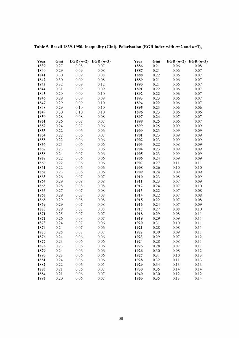
"
50
Table 5. Brazil 1839-1950. Inequality (Gini), Polarisation (EGR index with n=2 and n=3),
Year Gini EGR (n=2) EGR (n=3) Year Gini EGR (n=2) EGR (n=3) 1839 0.27 0.08 0.07 1886 0.21 0.06 0.08 1840 0.29 0.09 0.08 1887 0.21 0.06 0.07 1841 0.30 0.09 0.08 1888 0.22 0.06 0.07 1842 0.30 0.09 0.08 1889 0.21 0.06 0.07 1843 0.32 0.09 0.12 1890 0.21 0.06 0.07 1844 0.31 0.09 0.09 1891 0.22 0.06 0.07 1845 0.29 0.09 0.10 1892 0.22 0.06 0.07 1846 0.29 0.09 0.09 1893 0.23 0.06 0.07 1847 0.29 0.09 0.10 1894 0.22 0.06 0.07 1848 0.29 0.10 0.10 1895 0.23 0.06 0.06 1849 0.30 0.10 0.10 1896 0.23 0.06 0.06 1850 0.28 0.08 0.08 1897 0.24 0.07 0.07 1851 0.26 0.07 0.07 1898 0.25 0.06 0.07 1852 0.24 0.07 0.06 1899 0.25 0.09 0.09 1853 0.22 0.06 0.06 1900 0.23 0.09 0.09 1854 0.22 0.06 0.07 1901 0.23 0.09 0.09 1855 0.22 0.06 0.06 1902 0.23 0.09 0.09 1856 0.23 0.06 0.06 1903 0.22 0.08 0.09 1857 0.23 0.06 0.06 1904 0.23 0.09 0.09 1858 0.24 0.07 0.06 1905 0.23 0.09 0.09 1859 0.22 0.06 0.06 1906 0.24 0.09 0.09 1860 0.22 0.06 0.06 1907 0.27 0.11 0.11 1861 0.22 0.06 0.06 1908 0.26 0.10 0.10 1862 0.23 0.06 0.06 1909 0.24 0.09 0.09 1863 0.26 0.07 0.07 1910 0.23 0.08 0.09 1864 0.29 0.08 0.08 1911 0.23 0.07 0.09 1865 0.28 0.08 0.08 1912 0.24 0.07 0.10 1866 0.27 0.07 0.08 1913 0.22 0.07 0.08 1867 0.29 0.08 0.08 1914 0.22 0.07 0.08 1868 0.29 0.08 0.08 1915 0.22 0.07 0.08 1869 0.29 0.07 0.08 1916 0.24 0.07 0.09 1870 0.29 0.07 0.08 1917 0.27 0.08 0.10 1871 0.25 0.07 0.07 1918 0.29 0.08 0.11 1872 0.26 0.08 0.07 1919 0.29 0.09 0.11 1873 0.24 0.07 0.06 1920 0.31 0.10 0.11 1874 0.24 0.07 0.06 1921 0.28 0.08 0.11 1875 0.25 0.07 0.07 1922 0.30 0.09 0.11 1876 0.24 0.06 0.06 1923 0.29 0.07 0.12 1877 0.23 0.06 0.06 1924 0.28 0.08 0.11 1878 0.23 0.06 0.06 1925 0.28 0.07 0.11 1879 0.24 0.06 0.06 1926 0.30 0.08 0.12 1880 0.23 0.06 0.06 1927 0.31 0.10 0.13 1881 0.24 0.06 0.06 1928 0.32 0.11 0.13 1882 0.22 0.06 0.05 1929 0.34 0.13 0.13 1883 0.21 0.06 0.07 1930 0.35 0.14 0.14 1884 0.21 0.06 0.07 1940 0.30 0.12 0.12 1885 0.20 0.06 0.07 1950 0.35 0.13 0.14
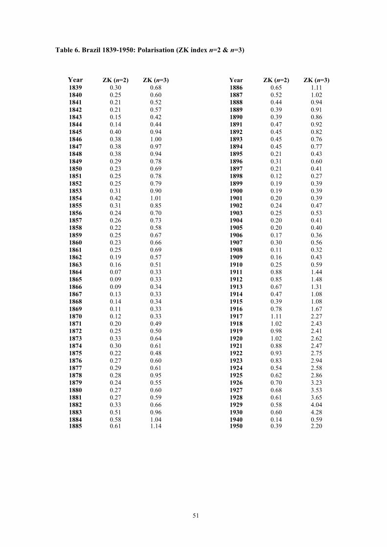
"
51
Table 6. Brazil 1839-1950: Polarisation (ZK index n=2 & n=3)
Year ZK (n=2) ZK (n=3) "" Year ZK (n=2) ZK (n=3) 1839 0.30 0.68 "" 1886 0.65 1.11 1840 0.25 0.60 "" 1887 0.52 1.02 1841 0.21 0.52 "" 1888 0.44 0.94 1842 0.21 0.57 "" 1889 0.39 0.91 1843 0.15 0.42 "" 1890 0.39 0.86 1844 0.14 0.44 "" 1891 0.47 0.92 1845 0.40 0.94 "" 1892 0.45 0.82 1846 0.38 1.00 "" 1893 0.45 0.76 1847 0.38 0.97 "" 1894 0.45 0.77 1848 0.38 0.94 "" 1895 0.21 0.43 1849 0.29 0.78 "" 1896 0.31 0.60 1850 0.23 0.69 "" 1897 0.21 0.41 1851 0.25 0.78 "" 1898 0.12 0.27 1852 0.25 0.79 "" 1899 0.19 0.39 1853 0.31 0.90 "" 1900 0.19 0.39 1854 0.42 1.01 "" 1901 0.20 0.39 1855 0.31 0.85 "" 1902 0.24 0.47 1856 0.24 0.70 "" 1903 0.25 0.53 1857 0.26 0.73 "" 1904 0.20 0.41 1858 0.22 0.58 "" 1905 0.20 0.40 1859 0.25 0.67 "" 1906 0.17 0.36 1860 0.23 0.66 "" 1907 0.30 0.56 1861 0.25 0.69 "" 1908 0.11 0.32 1862 0.19 0.57 "" 1909 0.16 0.43 1863 0.16 0.51 "" 1910 0.25 0.59 1864 0.07 0.33 "" 1911 0.88 1.44 1865 0.09 0.33 "" 1912 0.85 1.48 1866 0.09 0.34 "" 1913 0.67 1.31 1867 0.13 0.33 "" 1914 0.47 1.08 1868 0.14 0.34 "" 1915 0.39 1.08 1869 0.11 0.33 "" 1916 0.78 1.67 1870 0.12 0.33 "" 1917 1.11 2.27 1871 0.20 0.49 "" 1918 1.02 2.43 1872 0.25 0.50 "" 1919 0.98 2.41 1873 0.33 0.64 "" 1920 1.02 2.62 1874 0.30 0.61 "" 1921 0.88 2.47 1875 0.22 0.48 "" 1922 0.93 2.75 1876 0.27 0.60 "" 1923 0.83 2.94 1877 0.29 0.61 "" 1924 0.54 2.58 1878 0.28 0.95 "" 1925 0.62 2.86 1879 0.24 0.55 "" 1926 0.70 3.23 1880 0.27 0.60 "" 1927 0.68 3.53 1881 0.27 0.59 "" 1928 0.61 3.65 1882 0.33 0.66 "" 1929 0.58 4.04 1883 0.51 0.96 "" 1930 0.60 4.28 1884 0.58 1.04 " 1940 0.14 0.59 1885 0.61 1.14 "" 1950 0.39 2.20
""
European Historical Economics Society
!EHES!Working!Paper!Series Recent EHES Working Papers 2015 EHES.90 EHES.89 EHES.88 EHES.87 EHES.86 EHES.85 EHES.84 EHES.83
Spanish Land Reform in the 1930s: Economic Necessity or Political Opportunism? Juan Carmona, Joan R. Rosés and James Simpson Risen from Chaos: What drove the spread of Mass Education in the early 20th century China Pei Gao A city of trades: Spanish and Italian Immigrants in Late Nineteenth Century Buenos Aires. Argentina Leticia Arroyo Abad and Blanca Sánchez-Alonso A closer look at the long-term patterns of regional income inequality in Spain: the poor stay poor (and stay together) Daniel A. Tirado, Alfonso Díez-Minguela and Julio Martínez-Galarraga Did monetary forces cause the Hungarian crises of 1931? Flora Macher Did closures do any good? Labour productivity, mine dynamics, and rationalization in interwar Ruhr coal-mining Tobias A. Jopp Any lessons for today? Exchange-rate stabilization in Greece and South-East Europe between economic and political objectives and fiscal reality, 1841-1939 Matthias Morys Size and structure of disaster relief when state capacity is limited: China’s 1823 flood Ni Yuping and Martin Uebele
All papers may be downloaded free of charge from: www.ehes.org The European Historical Economics Society is concerned with advancing education in European economic history through study of European economies and economic history. The society is registered with the Charity Commissioners of England and Wales number: 1052680
Recommended