The Real Effect of the Initial Enforcement of Insider Trading Laws
Zhihong CHEN Hong Kong University of Science and Technology
Yuan HUANG Hong Kong Polytechnic University
Yuanto KUSNADI Singapore Management University
K.C. John WEI Hong Kong University of Science and Technology
The 7th NCTU International Finance Conference and
Celebration for Professor’s 40-year Teaching Career, January 10, 2014

Outline
• Research questions
• Motivation
• Theoretical analysis
• Research design
• Empirical results
• Conclusions and contributions
2

Research Questions
3
• How do regulations on insider trading affect a firm’s real investment decisions? – Use the initial enforcement of insider trading laws (the
enforcement) as an exogenous (to firms) shock of insider trading regulations.
• Does the enforcement affect the firm’s investment-to-price sensitivity? – If yes, what are the underlying mechanisms?
• Does the enforcement affect future firm performance? – If yes, is the enforcement’s effect on future performance
positively associated with its effect on the investment-to-price sensitivity?
Motivation
• Debates on the benefits and costs of insider trading regulation – Financial side (e.g., intensity and profitability of insider trading,
cost of equity, etc.)
– Information side (e.g., information acquisition, price efficiency, financial reporting quality, etc.)
– Real side (corporate investment)
• Understanding the real effect of insider trading regulation is important – Investment is the ultimate driving force of value creation
– Likely to have a first-order effect on welfare.
• There is little empirical evidence.
4

Preview of the Main Findings
• The sensitivity of investment to price is higher after the initial enforcement of insider trading laws
• A significant jump in the investment-to-price sensitivity occurred right after the enforcement.
• The increase in the investment-to-price sensitivity around the enforcement is – positively associated with the increase in the price informativenss for managers
around the enforcement.
– but not positively associated with the severity of agency problem and financial constraints before the enforcement.
• The accounting performance is improved after the enforcement. – The improvement is positively correlated with the increase in the investment-
to-price sensitivity after the enforcement.
5

The managerial learning hypothesis: the intuition
• The maintained assumption: – Outside investors have information about investment opportunity that is
unknown to managers.
– Such information is reflected in stock prices when the investors trade and the managers can learn from the stock prices.
• The mechanism – Investors have higher incentives to acquire and trade on private
information when insider trading is prohibited (i.e., after the enforcement) because they face less competition.
– Prices contain more information new to the managers after the enforcement.
– Value maximizing managers assign more weights to the stock prices when they estimate the investment opportunities.
– Corporate investment is more sensitive to the stock prices.
– Corporate investment is also more efficient.
6

The managerial learning hypothesis: A Simple Model
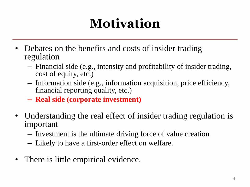
• Three stages
– t = 1
• Trading between informed investors, the manager (when insider trading is allowed), liquidity traders, and the market maker takes place in the security market.
• Equilibrium price is observed by the manager.
– t = 2
• The manager decide the amount of the investment based on all information available to her.
– t = 3
• The investment payoff is realized.
7
The Model Setup: The timeline
8
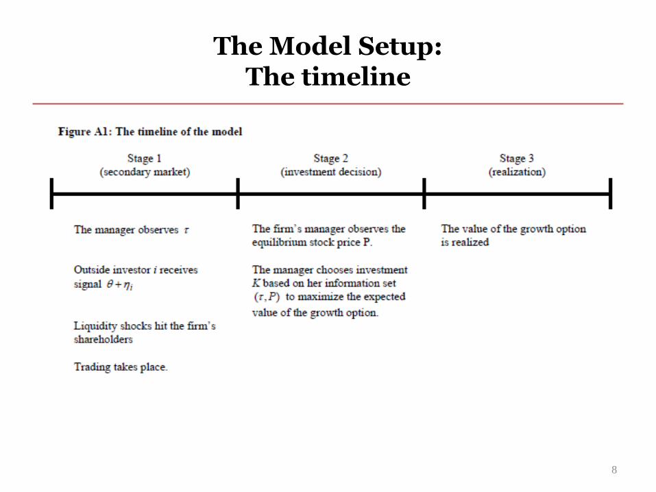
Model Setup: The firm and the information structure
9

The Model Setup: the trading procedure
• Follow Kyle (1985) and Admati and Pfleiderer (1988) to model the trading on the security market. – Liquidity traders’ demand is modeled as z~N(0,2
Z), where z is independent of , , i (i = 1, 2, …, m).
– The informed investors, the manager (when insider trading is allowed), and the liquidity traders submit market orders to the market maker.
– The market maker sets the share price and balances the supply and demand.
• Let R denote the regime regarding insider trading – R = I: insider trading is allowed
– R = N: insider trading is prohibited.
– Informed investors’ linear trading strategy XR(+i) = R(+i) (xi is the actual order placed).
– The manager’s linear trading strategy in regime I: Y() = (y is the actual order placed).
– The market maker’s linear pricing function: PR() = R(), where =xi+y+z.
10

The Model: Characterize the equilibrium
• The equilibrium
– Combination of trading strategy XR and Y, and a
pricing function PR such that
– XR maximizes the expected trading profit of the
informed investor: E[(+–p)xi|+i].
– Y maximizes the expected trading profit of the
manager: E[(+–p)y|].
– PR makes the market maker break even, i.e.,
PR()=E[+|], where = xi+y+z.
11

The equilibrium
12

The equilibrium
13

The price informativeness for managers
• Lemma 2
Define the informativeness of the stock price about as
R = var( |) – varR( |, P). Given m outside informed
investors, the stock price is more informative about
when insider trading is prohibited, i.e., N (m) > I (m).
• The equilibrium investment level is K*=+E(|,P)
– When P is more informative about , K* should be
more sensitive to P.
14
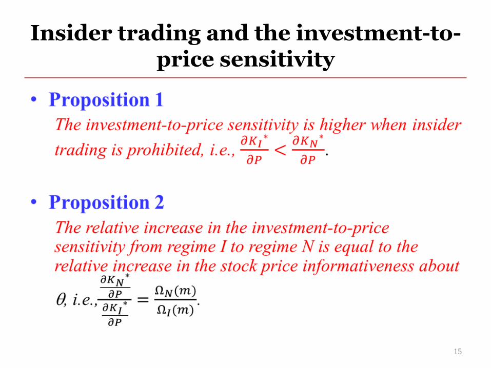
Insider trading and the investment-to-price sensitivity
15

Insider trading and the investment efficiency
16

Empirical Model Specification
INVEST: change in PPE plus change in inventories and plus R&D, scaled by
lagged total assets.
ITENF: =1 if year initial enforcement year; =0 otherwise
Q: Tobin’s Q, defined as market value of equity plus total assets minus book
value of equity, scaled by total assets.
CF: operating cash flows, defined as net income before extraordinary items
plus depreciation and amortization expenses, scaled by lagged total
assets.
c, i, and t: fixed effects of country, industry (2-digit SIC code) and year.
17
tfctic
tfctctfctfctctfc CFcITENFQbQbITENFaINVEST
,,
,,,,,,,,,,
11121111

Adjust for the trend in the investment-to-price sensitivity (Basic Idea)
• There might be a time-trend in the investment-to-price
sensitivity in the absence of the enforcement.
– INVESTt = b0Qt-1+btQt-1+ b1ITENF× Qt-1 + CONTROLS +
– Failing to control for this trend may result in erroneous
inference.
• Empirical approach to control for such trend
– INVESTt –btQt-1 = b0Qt-1 + b1ITENF× Qt-1 + CONTROLS +
• Define Adj.INVESTc,f,t = INVESTc,f,t – btQc,f,t-1 and use Adj.INVEST as the
dependent variable.
• Requires an estimate of bt for each year in the sample period.
18
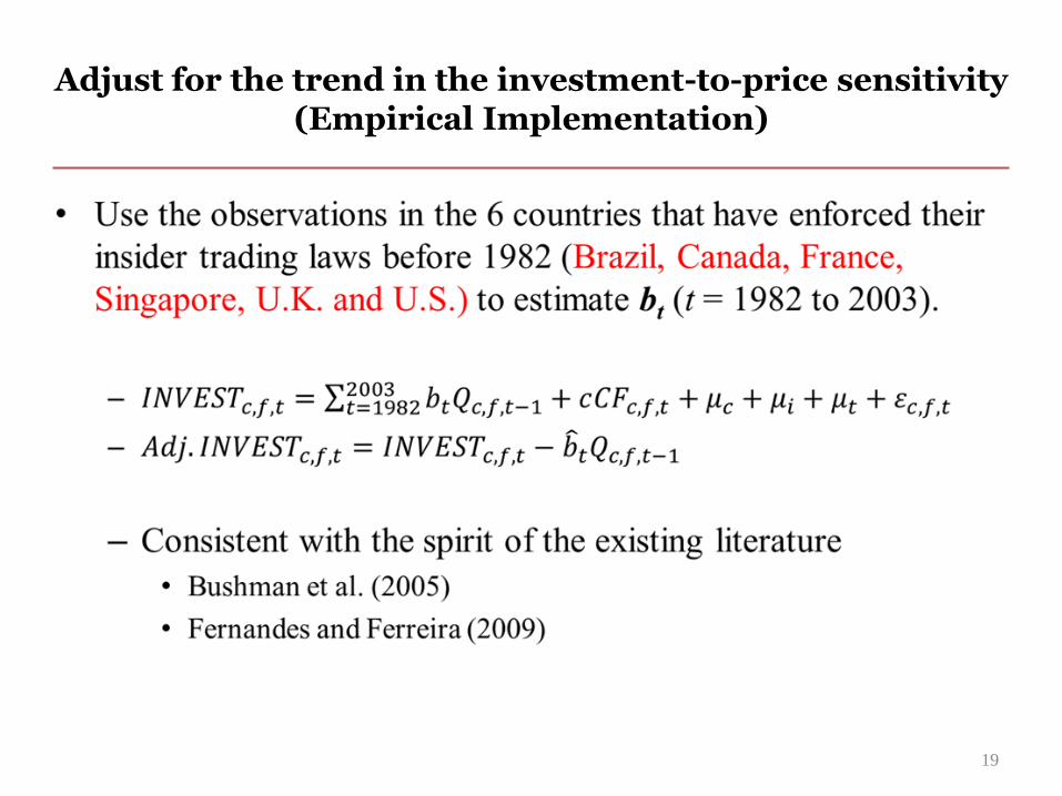
Adjust for the trend in the investment-to-price sensitivity (Empirical Implementation)
19
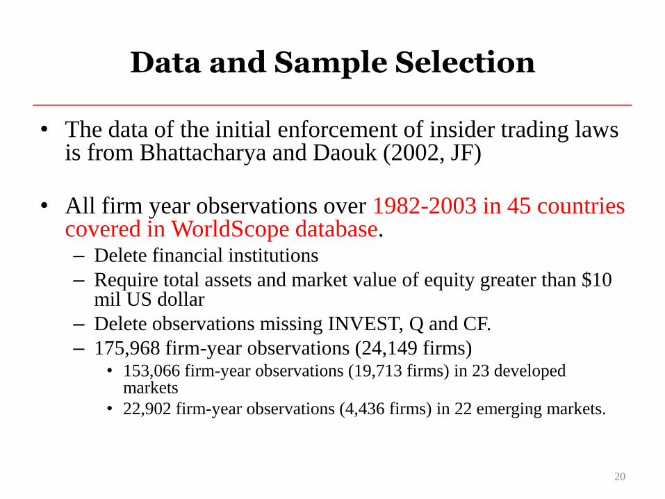
Data and Sample Selection
• The data of the initial enforcement of insider trading laws is from Bhattacharya and Daouk (2002, JF)
• All firm year observations over 1982-2003 in 45 countries covered in WorldScope database. – Delete financial institutions
– Require total assets and market value of equity greater than $10 mil US dollar
– Delete observations missing INVEST, Q and CF.
– 175,968 firm-year observations (24,149 firms) • 153,066 firm-year observations (19,713 firms) in 23 developed
markets
• 22,902 firm-year observations (4,436 firms) in 22 emerging markets.
20

Sample Distribution (Table 1)
21

Summary Statistics (Table 2)
22

Pooled Sample Regression (Table 3)
23

Event Window Analysis
• The pooled sample analysis includes observations far after the initial enforcement and thus allow other confounding factors to take effect.
• Only include observations in [T–2, T+3] – Year T is the actual enforcement year.
• [T–2, T] is the pre-enforcement period (ITENF=0)
• [T+1, T+3] is the post-enforcement period (ITENF=1).
• The country has at least one observation in both the pre- and the post-enforcement periods.
• 19293 firm-year observations (5023 firms).
– Repeat the regression in Table 3.
24

Event Window Analysis (Table 4)
25

Year by year change of the Investment-to-Price sensitivity in the event window
• YEARc,t,: dummy variable equals one for all firms in country c if year t is years ( [-1,+3]) relative to country c’s initial enforcement year, and zero
otherwise.
– Event year -2 ( = -2) serves as the benchmark year.
– The investment-to-price sensitivity in year -2 is captured by coefficient b.
• Coefficient estimates of b ( [-1,+3]) measure the difference in the
trend-adjusted investment-to-price sensitivity between event year and
event year -2.
26
tfcictfc
tctfctfctctfc
cCF
YEARQbbQYEARINVESTAdj
,,,,
,,,,,,,,,,
.
3
1
3
111

The change in the trend-adjusted investment-to-price sensitivity around the initial enforcement of insider trading laws
(Figure 1)
27

Benchmark against the empirical distribution based on pseudo-enforcement events
• For each country, randomly select a year t as a pseudo enforcement year. – Use the observations in [t-2, t+3] to repeat the analysis of Table 5 and
Figure 1. • [t-2, t]: pre-pseudo-enforcement period. ITENF=0.
• [t+1, t+3]: post-pseudo-enforcement period. ITENF=1.
• Estimate the coefficients of Q×ITENF and Q×YEAR1–Q×YEAR0.
– t [T-3, T+3], where T is the actual enforcement year • The pseudo-event sample period does not overlap with the actual enforcement
year.
• Repeat the random sampling for 1000 times. – Use the empirical distribution of the coefficients of Q×ITENF and
Q×YEAR1–Q×YEAR0 to gauge the corresponding coefficient estimates in Table 4 and Figure 1.
28

Benchmark against empirical distribution based on pseudo-enforcement events
29
Coefficient of Q×ITENF
(dependent variable is Adj.INVEST)
Estimate in model (1) of Table 4 0.013
99% confidence interval (i.e., [0.5th
percentile, 99.5th percentile] based on the
empirical distribution
[-0.014, 0.011]
Coefficient of Q×YEAR1–Q×YEAR0
(dependent variable is Adj.INVEST)
Estimate in Figure 1 0.019
(0.011 + 0.008)
99% confidence interval (i.e., [0.5th
percentile, 99.5th percentile] based on the
empirical distribution
[-0.015, 0.017]

Economic Significance (based on the pooled sample regression results)
• Define the excess investment-to-price sensitivity as the raw sensitivity of the sample firms minus that of the six benchmark countries in the same year.
• The excess sensitivity is increased by 0.007, or 25% (0.007/0.028).
• Compared with the six benchmark countries, in the sample countries, – Before the enforcement, the increase in the
investment associated with one-standard-deviation increase in Q (0.999) is 0.028 smaller,
– The discrepancy is reduced to 0.021 (0.028 – 0.007) after the enforcement.
• The difference is about 9.5% of the mean investment (0.007/0.074).
30

Economic Significance (based on the event window regression results)
• The excess sensitivity is increased by 0.013, or 30% (0.013/0.043).
• Compared with the six benchmark countries, in the sample countries, – Before the enforcement, the increase
in the investment associated with one-standard-deviation increase in Q (0.999) is 0.043 smaller,
– The discrepancy is reduced to 0.03 (0.043 – 0.013) after the enforcement.
• The difference is about 18% of the mean investment (0.013/0.074).
31

Robustness Tests: alternative model specifications (Table 5)
32
Column Robustness tests
(1) Firm fixed effects regression
(2) Exclude the Asian financial crisis period (year 1997 and 1998).
(3) Exclude influential countries (Germany and Japan).
(4) Cluster standard errors by country.
(5) Controlling for investor protection and per capita GDP.
(6) Country level analysis.

Country level analysis
33
• Two-step regressions
– First step, estimate the following annual regression for each
country-year with at least 50 firms
Adj.INVESTc,f,t = bc,t Qc,f,t-1+ cc,t CFc,f,t+ industry fixed effects+ c,f,t
– Second step, estimate the following regression
bc,t=0+1ITENFc,t-1+c+c,t

Alternative Model Specification: pooled sample regression (Table 5, Panel A)
34

Alternative Model Specification: event-window regression (Table 5, Panel B)
35

Robustness Tests: alternative measure of investment (Table 6)
36
Column Definition of investments
(1) Change in PPE divided by lagged total assets.
(2) (Change in PPE plus R&D) divided by lagged total assets.
(3) (Change in PPE plus R&D plus change in inventory) divided by
current period total assets.
(4) (Change in PPE plus R&D plus change in inventory) divided by
lagged PPE.
(5) Capital expenditure (CAPX) divided by lagged PPE.

Alternative Measures of Investment: Pooled sample regression (Table 6, Panel A)
37

Alternative Measures of Investment: Event window regression (Table 6, Panel B)
38

The managerial learning hypothesis
• Proposition 2
– The increase in the investment-to-price sensitivity should be positively associated with the relative increase in the price informativeness for managers around the enforcement year.
• Price informativeness for managers is not directly observable.
– Use firm characteristics that suggest a greater increase in price informativeness for managers.
39

Empirical Design
40
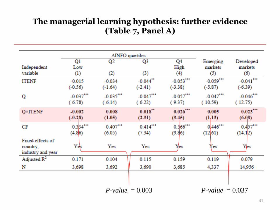
The managerial learning hypothesis: further evidence (Table 7, Panel A)
41
P-value = 0.003 P-value = 0.037
The change in public information quality and the enforcement effect
• INFO may proxy for public information quality. – Jin and Myers (2006, JFE); Hutton, Marcus, and Tehranian
(2009, JFE)
• INFO may capture the change in public information quality
• To address this concern, we partition the sample based on a more direct measure of public information quality. – Measure public information quality by the negative of the
absolute value discretionary accruals (FRQ).
– Higher FRQ implies better financial reporting quality and thus better public information quality.
– Compute FRQ as the mean value of FRQ over year 0 to +2 minus the mean value over year -3 to -1.
– Partition the sample based on FRQ.
42

Public information quality and the effect of the enforcement (Table 7, Panel B)
43

Alternative Explanation: The market friction hypothesis
• The enforcement reduces market frictions by mitigating moral hazard and/or adverse selection problems.
• The enforcement reduces the cost of external finance and relaxes the external financing constraints.
• If this is the case, then the effect of the enforcement should be more pronounced – when firms have more severe agency problems before the
enforcement
– when firms are more financially constrained before the enforcement.
44

Controlling shareholders’ incentives and the effect of the enforcement
(Table 8)
45

The effect of the enforcement on accounting performance
• We proxy the expected value of growth by future accounting performance
• Proposition 3
– Future accounting performance improves after the enforcement.
• Proposition 4
– The improvement in future accounting performance is positively associated with the increase in the investment-to-price sensitivity after the enforcement.
46

The effect of the enforcement on accounting performance
47
tfcctctcttfc CONTROLsQSENSITENFaITENFaPERFORM ,,,,],[,, 2131
.
.
,,,,
,,,
,,,,,
tfcictfc
ctcctfcc
cctfcc
ctccctfc
cCF
ITENFCOUNTRYQQSENS
COUNTRYQbITENFCOUNTRYaINVESTAdj
11
11

The Initial Enforcement of Insider Trading Laws and Accounting Performance
(Table 9)
48

Conclusions and contributions
• Investment becomes more sensitive to prices after the enforcement.
• A significant jump in the investment-to-price sensitivity occurred right after the enforcement.
• The managerial learning hypothesis seems best explain the results.
• Improvement in accounting performance after the enforcement is positively associated with the increase in the investment-to-price sensitivity.
49
Conclusions and contributions
• The first large sample empirical study on the real-side effect of insider trading regulation. – Shed light on the long-lasting analytical debates on the real effect of insider
trading regulation.
– Extend the studies on insider trading regulation from financial side, information side to the real side of the economy.
– Identify the channel.
• Contribute to the effect of country-level legal, institutional and regulatory factors on corporate investment. – Most other country level factors affect corporate investment primarily by
mitigating adverse selection and moral hazard problems.
– Insider trading regulation takes effect by a different channel.
• Contribute to the learning literature. – Document how insider trading regulation affects managerial learning in an
international setting.
50
Recommended