i
Abstract
This thesis describes a psychophysical experiment carried out to assess the perceptual
influence of approximating ambient occlusion in real-time rendering. Three different
screen-space ambient occlusion techniques of differing physical accuracy were
implemented for the experiment. The results of the experiment show that screen-
space ambient occlusion can increase the perceived realism of visually complex
synthetic images. Visual complexity was also found to have an influence on the
required physical accuracy of the ambient occlusion algorithm. Specifically, as the
visual complexity increases, the required physical accuracy of ambient occlusion
decreases. In a visually complex, ecologically valid scenario, experiment participants
were not able to discern a difference between two different screen-space ambient
occlusion techniques with significant observable quality differences. The results of
the experiment suggest that in practical application scenarios such as computer
games, it is prudent to investigate the need for, and impact of, screen-space ambient
occlusion for individual scenes or environments. In many cases, low accuracy
ambient occlusion can be sufficient, and in some cases it can be turned off
completely; thus allowing for more computation time to be utilized on other
perceptually important rendering tasks.

ii
This page is intentionally left blank
iii
Preface
This thesis was made at Aalborg University Copenhagen in fulfilment of the
requirements for acquiring the Master of Science degree in Medialogy, M.Sc.
Medialogy. Work on the thesis was carried out over a period of four months
constituting a full semester and 30 ECTS points.
The contents of the thesis constitute advanced topics in computer graphics
programming and so it is assumed that the reader possesses knowledge comparable to
a bachelor in Computer Science.
The thesis comes with a CD holding this report and appendix materials that are not
included in the printed appendix (such as code and stimuli images). The CD contains
a readme file explaining the file structure and all the contents included.
The thesis is divided into six distinct chapters. The first chapter constitutes the
introduction and outlines the background of the thesis as well as the motivation and
goal. Chapter 2 describes work relevant for the thesis, while chapter 3 covers the
theory necessary for carrying out the implementation detailed in chapter 4. Chapter 5
covers the details of setting up and carrying out a psychophysical experiment while
chapter 6 rounds up the thesis with a discussion and conclusion.
Aalborg University Copenhagen, May 2010
Christian Jakobsen

iv
Acknowledgements
I would like to thank Daniel Grest for supervision and guidance; Crytek GmbH for
creating the Sponza model and textures used in the experiment and making it
available to the general public; and both Crytek and Blizzard Entertainment for
making their ambient occlusion algorithms available to the public.
v
Table of Contents
Preface ........................................................................................................................... i
Acknowledgements .................................................................................................... iv
Table of Contents ........................................................................................................ v
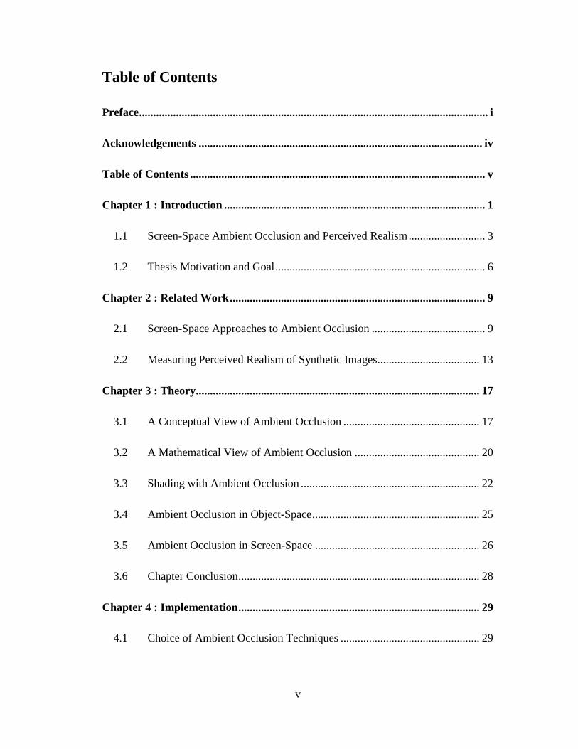
: Introduction ............................................................................................ 1 Chapter 1
1.1 Screen-Space Ambient Occlusion and Perceived Realism ........................... 3
1.2 Thesis Motivation and Goal .......................................................................... 6
: Related Work .......................................................................................... 9 Chapter 2
2.1 Screen-Space Approaches to Ambient Occlusion ........................................ 9
2.2 Measuring Perceived Realism of Synthetic Images.................................... 13
: Theory.................................................................................................... 17 Chapter 3
3.1 A Conceptual View of Ambient Occlusion ................................................ 17
3.2 A Mathematical View of Ambient Occlusion ............................................ 20
3.3 Shading with Ambient Occlusion ............................................................... 22
3.4 Ambient Occlusion in Object-Space ........................................................... 25
3.5 Ambient Occlusion in Screen-Space .......................................................... 26
3.6 Chapter Conclusion ..................................................................................... 28
: Implementation ..................................................................................... 29 Chapter 4
4.1 Choice of Ambient Occlusion Techniques ................................................. 29
vi
4.2 Implementing a Suitable Rendering Framework ........................................ 30
4.3 Implementing the Ambient Occlusion Techniques ..................................... 35
4.3.1 Crytek Technique .................................................................................... 36
4.3.2 Blizzard Technique ................................................................................. 41
4.3.3 Ray-Marching Technique ....................................................................... 47
4.3.4 Techniques Comparison and Discussion ................................................ 48
4.4 Additional Implementation Considerations ................................................ 49
: Experiment Procedure and Results ................................................... 51 Chapter 5
5.1 Experimental Hypotheses ........................................................................... 51
5.2 Experiment Procedure ................................................................................. 52
5.3 Creating the Experiment Stimuli ................................................................ 54
5.3.1 Low Ecological Validity ......................................................................... 55
5.3.2 Moderate Ecological Validity ................................................................. 56
5.3.3 High Ecological Validity ........................................................................ 58
5.4 The Experiment ........................................................................................... 59
5.5 The Results.................................................................................................. 62
5.5.4 Low Ecological Validity Results ............................................................ 62
5.5.5 Moderate Ecological Validity Results .................................................... 62
5.5.6 High Ecological Validity Results............................................................ 62
vii
5.6 Statistical Analysis ...................................................................................... 64
: Discussion & Conclusion..................................................................... 67 Chapter 6
6.1 Discussion ................................................................................................... 67
6.1.1 Prominent Results ................................................................................... 68
6.1.2 Stimuli Design ........................................................................................ 69
6.1.3 Experiment Procedure ............................................................................. 70
6.1.4 Insights on Ambient Occlusion ............................................................... 71
6.2 Conclusion .................................................................................................. 72
6.2.5 Broader Implications and Thesis Contribution ....................................... 73
6.3 Future Work ................................................................................................ 73
Appendix A: Crytek Ambient Occlusion Code ...................................................... 75
Appendix B: Blizzard Ambient Occlusion Code .................................................... 77
Appendix C: Ray-Marching Ambient Occlusion Code ......................................... 79
Appendix D: Experiment Instructions .................................................................... 82
Appendix E: Stimuli Pair I – Dragon Low ............................................................. 83
Appendix F: Stimuli Pair II – Sponza Moderate ................................................... 84
Appendix G: Stimuli Pair III – Sponza Moderate ................................................. 85
Appendix H: Stimuli Pair IV – Characters Moderate .......................................... 86
Appendix I: Stimuli Pair V – Sponza High ............................................................ 87

viii
Appendix J: Stimuli Pair VI – Sponza High .......................................................... 88
Appendix K: Stimuli Pair VII – Characters High ................................................. 89
Glossary ..................................................................................................................... 90
Bibliography .............................................................................................................. 93
1
: Introduction Chapter 1
Striving for realism in real-time rendering is a difficult proposition at best. The
amount of calculations required to match how light interacts in the real world is
staggering and completely impractical for real-time purposes. Even in off-line
rendering scenarios such as film and television production, where several hours or
more can be dedicated to rendering a single frame of animation, approximations to
how light behaves are often preferred in lieu of physical accuracy in order to cut
down on rendering time. For example, ILM adapted an approach developed for real-
time rendering as part of their global illumination pipeline in production of Pirates of
the Caribbean (Robertson 2006). The use of approximations is of course even more
relevant in real-time rendering scenarios where the time to render a single frame is
reduced to a scale of milliseconds. Until recently, lighting in real-time rendering
scenarios such as computer games has consisted of local illumination models only,
with global illumination effects such as visibility determination and indirect light
transport either being omitted, or pre-computed using techniques such as light maps
and occlusion maps.
When using local illumination models in rendering, light is emitted from a light
source and only surfaces that are directly visible from the light source are illuminated.
In the real world, some of the light would be reflected or transmitted and proceed to
illuminate other surfaces in the environment. This indirect light transport is a very
important element of convincingly lighting a synthetic scene, but is unfortunately also
a prohibitively expensive process for real-time rendering. Methods such as photon
mapping (Jensen 1996) and radiosity (Goral, et al. 1984) are popular solutions in
offline rendering scenarios, but graphics hardware have not yet progressed to the
point where such solutions are feasible for time-critical applications such as computer
games. Instead, these techniques are often employed as a pre-processing step,
computed and stored in a light map which is later used in real-time to modulate the
illumination a surface receives. This is a common trend, to approach the problem of
global illumination in a piecemeal fashion, using a divide and conquer approach to
2
separate the complex problem of calculating the global illumination in a synthetic
scene into smaller, more manageable problems. For example, using radiosity to
calculate a light map only accounts for inter-diffuse reflections, but not other global
illumination phenomena such as caustics and shadows. An important step that is
omitted here is visibility determination which evaluates whether or not a shaded point
can see another point and consequently, whether any indirect illumination should be
calculated between those two points.
With the rapid increase in computing power offered by newer generations of
graphical processing units, developers and academics alike have seen the possibilities
of developing and implementing ever more flexible and accurate approximations to
isolated global illumination phenomena. The research into this area can roughly be
divided into two major categories; algorithms that work in object-space, and
algorithms that work in screen-space. Techniques falling into the former category
usually employ ray-tracing and full knowledge of the scene structure to calculate the
light transport in a given scene, and have recently progressed into the realm of
interactive frame rates, e.g. (Wang, et al. 2009). While this is an area of research that
hold exiting potential for future applications; graphics hardware have not yet
progressed to the point where such implementations can offer sufficient frame rates
for more time critical applications such as computer games.
On the other hand, the category of screen-space approaches offers much faster
techniques, operating only on visible pixels that have passed the depth test making it
largely independent of scene complexity. Working on a limited data set instead of the
full scene structure of course implies that techniques performed in screen-space are
more coarse approximations of the real-world phenomena. A recent technique that
have become popular in both literature and the computer games industry, commonly
referred to as “Screen-Space Ambient Occlusion”, make some clever assumptions
regarding how much indirect diffuse light a sample point is receiving based on nearby
surrounding geometry. The result of applying ambient occlusion to indirect lighting is
a darkening of areas where there is a lot of surrounding geometry. This provides
3
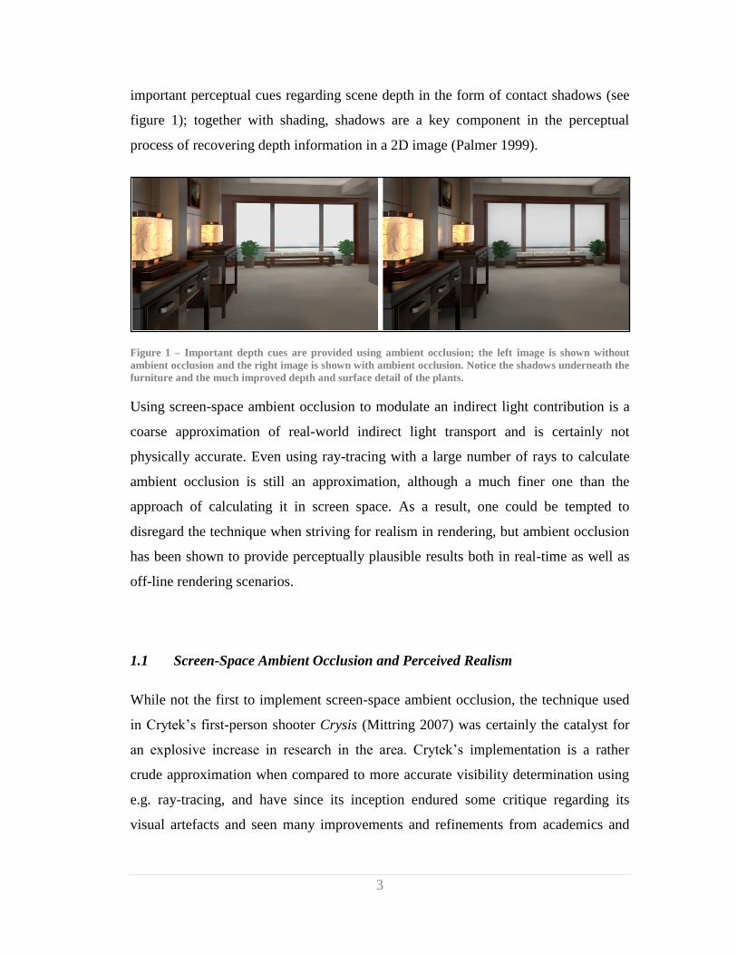
important perceptual cues regarding scene depth in the form of contact shadows (see
figure 1); together with shading, shadows are a key component in the perceptual
process of recovering depth information in a 2D image (Palmer 1999).
Figure 1 – Important depth cues are provided using ambient occlusion; the left image is shown without
ambient occlusion and the right image is shown with ambient occlusion. Notice the shadows underneath the
furniture and the much improved depth and surface detail of the plants.
Using screen-space ambient occlusion to modulate an indirect light contribution is a
coarse approximation of real-world indirect light transport and is certainly not
physically accurate. Even using ray-tracing with a large number of rays to calculate
ambient occlusion is still an approximation, although a much finer one than the
approach of calculating it in screen space. As a result, one could be tempted to
disregard the technique when striving for realism in rendering, but ambient occlusion
has been shown to provide perceptually plausible results both in real-time as well as
off-line rendering scenarios.
1.1 Screen-Space Ambient Occlusion and Perceived Realism
While not the first to implement screen-space ambient occlusion, the technique used
in Crytek‟s first-person shooter Crysis (Mittring 2007) was certainly the catalyst for
an explosive increase in research in the area. Crytek‟s implementation is a rather
crude approximation when compared to more accurate visibility determination using
e.g. ray-tracing, and have since its inception endured some critique regarding its
visual artefacts and seen many improvements and refinements from academics and
4
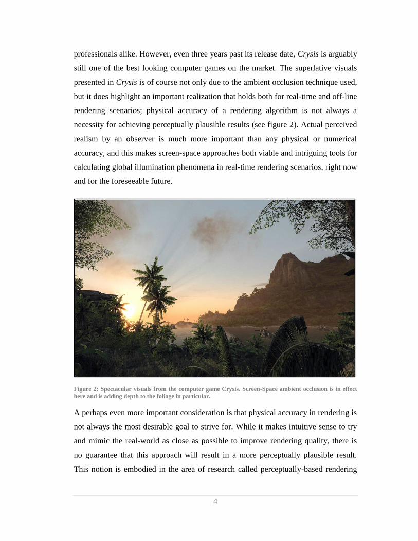
professionals alike. However, even three years past its release date, Crysis is arguably
still one of the best looking computer games on the market. The superlative visuals
presented in Crysis is of course not only due to the ambient occlusion technique used,
but it does highlight an important realization that holds both for real-time and off-line
rendering scenarios; physical accuracy of a rendering algorithm is not always a
necessity for achieving perceptually plausible results (see figure 2). Actual perceived
realism by an observer is much more important than any physical or numerical
accuracy, and this makes screen-space approaches both viable and intriguing tools for
calculating global illumination phenomena in real-time rendering scenarios, right now
and for the foreseeable future.
Figure 2: Spectacular visuals from the computer game Crysis. Screen-Space ambient occlusion is in effect
here and is adding depth to the foliage in particular.
A perhaps even more important consideration is that physical accuracy in rendering is
not always the most desirable goal to strive for. While it makes intuitive sense to try
and mimic the real-world as close as possible to improve rendering quality, there is
no guarantee that this approach will result in a more perceptually plausible result.
This notion is embodied in the area of research called perceptually-based rendering

5
(McNamara 2001). Perceptually-based rendering methods attempt to exploit the
limitations of the human visual system to speed up rendering algorithms.
Conceptually, the idea is to identify areas of high perceptual saliency in a synthetic
image and focus computational power on these areas thus improving rendering
quality by maximizing the time dedicated to perceptually important areas of the
image. Whether this approach is consciously followed from a development point of
view or not, the idea is often the basis for real-time rendering algorithms; born out of
shear necessity for attaining real-time frame rates. The validity of a perceptually
based approach is often determined either by using the visual difference predictor
(Daly 1993) or a similar algorithm to map out the overall perceivable pixel error of
the rendered image; or by conducting a psychophysical study on human observers
comparing images side by side. For an example of both see (McNamara 2006). Either
approach presupposes a ground truth or a gold standard image to which the
approximation is compared.
While a comparative study of selective renderings and a real world or synthetic
ground truth reference image can state a lot about the physical accuracy of a given
rendering algorithm, it does not necessarily reveal anything useful about how
perceptually realistic an image produced by a given algorithm is. In addition, the
ground truth comparative study scenario is an inherently contrived experimental
scenario that essentially has no real world correlate, that is to say; when experiencing
computer generated imagery, whether it be in a movie or computer game or some
other source, we rarely have a reference on hand to compare the realism of the
displayed images with. One notable exception to this is the compositing of live action
footage and computer generated imagery in film and television. In this case, it can
make sense to attempt to maximize physical accuracy of the rendering algorithms
used, since the final rendered images has to match the live action footage in quality
and appearance. In real-time rendering scenarios there is no such comparison taking
place, and the final arbiter on realism or rendering quality is how it is perceived by a
human observer alone, not how it compares to real footage.
6
1.2 Thesis Motivation and Goal
This thesis is partly motivated by the observation that visibility approximations such
as ambient occlusion have been shown to provide perceptually realistic results despite
showing clear perceptible differences to “ground truth” reference images (Yu, et al.
2009). Additionally, as mentioned in the previous section ambient occlusion has
become a popular topic in contemporary real-time rendering scenarios, especially
computer games; but it is not clear what the perceptual influence of ambient
occlusion is on perceived realism.
The aim of the thesis is to conduct a formal study into the perceptual characteristics
of approximating global illumination phenomena in screen-space. More specifically,
the goal of the study is to measure the effect of screen-space ambient occlusion on the
perceived realism of a synthetic image. In order to make the subject amenable for
experimental testing, the focus of the study is limited to visibility approximations in
screen-space.
The main contribution of the thesis is a psychophysical study into the perceptual
influence of using screen-space ambient occlusion in a real-time rendering context. In
the literature, several studies have set out to measure the perceived realism of
synthetic images created using different rendering algorithms (Yu, et al. 2009)
(Sundstedt, et al. 2007) (Kozlowski and Kautz 2007) (Jimenez, Sundstedt and
Gutierrez 2009), however, no such investigations have yet been carried out on the
perceptual influence of screen-space ambient occlusion. Moreover, many perceptual
studies involve experiments revolving around the ground truth reference scenario,
where stimuli sets are subject to direct comparison. This study takes a different
approach in an effort to map out the perceptual influence of screen space ambient
occlusion in a more ecologically valid context; by carrying out a no-reference
experiment with visually complex stimuli. The no-reference experiment denotes a
comparison task between two images where no direct comparison is allowed, i.e.
subjects are not allowed to view images side by side or flip back and forth between
them.
7
In order to assess the perceptual influence of screen-space ambient occlusion on the
perceived realism of synthetic images, three different ambient occlusion techniques of
differing physical accuracy are included in the study along with a no-occlusion
scenario. These four techniques are integrated into a variety of contexts varying in
geometric complexity and lighting conditions, thus exhibiting different levels of
ecological validity (higher visual complexity results in higher ecological validity);
and are then compared to each other in different no-reference experimental scenarios.
The purpose of comparing the no-occlusion scenario with an occlusion scenario is to
assess whether subjects can perceive a difference, while the inter-comparison
between occlusion techniques is to determine whether physical accuracy of the
ambient occlusion has any bearing on perceived realism. These research goals are
posited in a more formal manner in chapter 5.
The following chapter outlines previous work deemed relevant for the thesis, both in
the area of screen-space visibility approximations and the area of psychophysics
governing the measurements of perceptual phenomena. In chapter 3, the theory
regarding ambient occlusion necessary for setting up and carrying out the ensuing
experiment is covered. Chapter 4 goes into the technical details of implementing
screen-space occlusion techniques in a suitable rendering framework while chapter 5
details the experimental procedure as well as presenting the results of the experiment.
Chapter 6 is dedicated to the discussion and conclusion.

8
This page is intentionally left blank.
9
: Related Work Chapter 2
Previous work relevant to this thesis can be divided into two major categories. The
first category is research and development of algorithms for approximating ambient
occlusion in screen-space. The second category is research into the perceived realism
or fidelity of synthetic images. Most relevant in the latter category is research that
deals with the perception of visibility approximations such as ambient occlusion, but
given that such research is sparse, key contributions on measuring perceived realism
of synthetic images in general are also described. This chapter contains two sections
outlining relevant work in these two categories.
Because the following section deals with screen-space approaches to computing
ambient occlusion in general, previous knowledge about ambient occlusion is
assumed. If the reader is unfamiliar with screen-space approaches to ambient
occlusion, or just ambient occlusion in general, it is recommended to review chapter 3
first, which covers ambient occlusion from theoretical concept to practical
implications.
2.1 Screen-Space Approaches to Ambient Occlusion
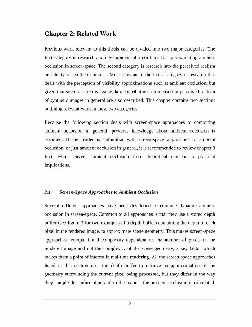
Several different approaches have been developed to compute dynamic ambient
occlusion in screen-space. Common to all approaches is that they use a stored depth
buffer (see figure 3 for two examples of a depth buffer) containing the depth of each
pixel in the rendered image, to approximate scene geometry. This makes screen-space
approaches‟ computational complexity dependent on the number of pixels in the
rendered image and not the complexity of the scene geometry, a key factor which
makes them a point of interest in real-time rendering. All the screen-space approaches
listed in this section uses the depth buffer to retrieve an approximation of the
geometry surrounding the current pixel being processed, but they differ in the way
they sample this information and in the manner the ambient occlusion is calculated.
10
Some approaches also make use of surface normals at sampled points to further
improve the results.
In the following, key screen-space ambient occlusion techniques are presented and
briefly reviewed. This section constitutes a somewhat cursory look at relevant
ambient occlusion techniques. A more thorough and in depth look at the theory
underlying ambient occlusion is presented in chapter 3.
Figure 3: Two examples of a depth buffer. The depth buffer holds the depth values of all the pixels found
closest to the camera. Black represents depths closest to the camera with white representing the furthest
distance from the camera.
Because screen-space approaches operate on a per-pixel basis, but also samples pixels
around the current pixel being processed, there can be some confusion in
terminology. To aid in understanding, the term “pixel position” refers to the position
of the current pixel being processed, that is, the pixel for which the ambient occlusion
is being calculated. The term “sample position” and “sample point” refers to the
pixels or 3D positions being sampled around the pixel position to compute the
occlusion.
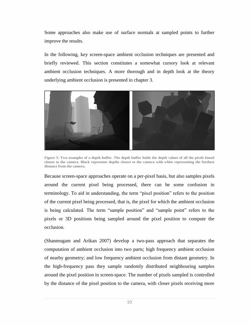
(Shanmugam and Arikan 2007) develop a two-pass approach that separates the
computation of ambient occlusion into two parts; high frequency ambient occlusion
of nearby geometry; and low frequency ambient occlusion from distant geometry. In
the high-frequency pass they sample randomly distributed neighbouring samples
around the pixel position in screen-space. The number of pixels sampled is controlled
by the distance of the pixel position to the camera, with closer pixels receiving more
11
samples to provide better detail. To calculate the amount of occlusion contributed by
each sample around the pixel position, a spherical proxy is used with an inverse
square falloff to scale the occlusion with the distance of the occluding sample. The
low frequency pass differs in that it uses actual geometry, also in the form of spheres,
to compute the ambient occlusion. This pass is less flexible than the high-frequency
pass as well as the other approaches mentioned in the following, in that it requires
special preparation of the scene. Essentially, a second version of the scene has to be
created that approximates the surface geometry of the original scene using geometric
spheres. For animated scenes, the positions of the spheres are recalculated each frame
based on the vertex positions of the geometry they are approximating. Figure 4 shows
an example of their approach with a before and after image.
Figure 4: A before and after example of the approach by (Shanmugam and Arikan 2007). Note that this is a
somewhat contrived example in that the before shot is only receiving constant ambient illumination.
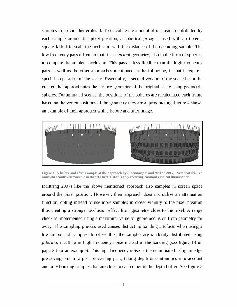
(Mittring 2007) like the above mentioned approach also samples in screen space
around the pixel position. However, their approach does not utilise an attenuation
function, opting instead to use more samples in closer vicinity to the pixel position
thus creating a stronger occlusion effect from geometry close to the pixel. A range
check is implemented using a maximum value to ignore occlusion from geometry far
away. The sampling process used causes distracting banding artefacts when using a
low amount of samples; to offset this, the samples are randomly distributed using
jittering, resulting in high frequency noise instead of the banding (see figure 13 on
page 28 for an example). This high frequency noise is then eliminated using an edge
preserving blur in a post-processing pass, taking depth discontinuities into account
and only blurring samples that are close to each other in the depth buffer. See figure 5
12
on the left for an example of the ambient occlusion buffer resulting from this
approach.
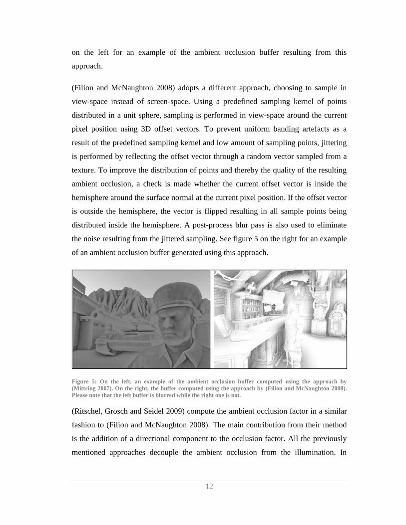
(Filion and McNaughton 2008) adopts a different approach, choosing to sample in
view-space instead of screen-space. Using a predefined sampling kernel of points
distributed in a unit sphere, sampling is performed in view-space around the current
pixel position using 3D offset vectors. To prevent uniform banding artefacts as a
result of the predefined sampling kernel and low amount of sampling points, jittering
is performed by reflecting the offset vector through a random vector sampled from a
texture. To improve the distribution of points and thereby the quality of the resulting
ambient occlusion, a check is made whether the current offset vector is inside the
hemisphere around the surface normal at the current pixel position. If the offset vector
is outside the hemisphere, the vector is flipped resulting in all sample points being
distributed inside the hemisphere. A post-process blur pass is also used to eliminate
the noise resulting from the jittered sampling. See figure 5 on the right for an example
of an ambient occlusion buffer generated using this approach.
Figure 5: On the left, an example of the ambient occlusion buffer computed using the approach by
(Mittring 2007). On the right, the buffer computed using the approach by (Filion and McNaughton 2008).
Please note that the left buffer is blurred while the right one is not.
(Ritschel, Grosch and Seidel 2009) compute the ambient occlusion factor in a similar
fashion to (Filion and McNaughton 2008). The main contribution from their method
is the addition of a directional component to the occlusion factor. All the previously
mentioned approaches decouple the ambient occlusion from the illumination. In
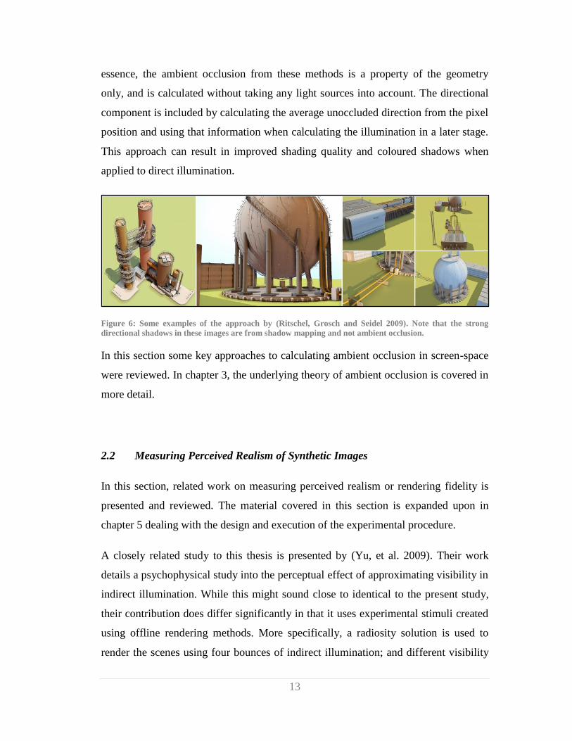
13
essence, the ambient occlusion from these methods is a property of the geometry
only, and is calculated without taking any light sources into account. The directional
component is included by calculating the average unoccluded direction from the pixel
position and using that information when calculating the illumination in a later stage.
This approach can result in improved shading quality and coloured shadows when
applied to direct illumination.
Figure 6: Some examples of the approach by (Ritschel, Grosch and Seidel 2009). Note that the strong
directional shadows in these images are from shadow mapping and not ambient occlusion.
In this section some key approaches to calculating ambient occlusion in screen-space
were reviewed. In chapter 3, the underlying theory of ambient occlusion is covered in
more detail.
2.2 Measuring Perceived Realism of Synthetic Images
In this section, related work on measuring perceived realism or rendering fidelity is
presented and reviewed. The material covered in this section is expanded upon in
chapter 5 dealing with the design and execution of the experimental procedure.
A closely related study to this thesis is presented by (Yu, et al. 2009). Their work
details a psychophysical study into the perceptual effect of approximating visibility in
indirect illumination. While this might sound close to identical to the present study,
their contribution does differ significantly in that it uses experimental stimuli created
using offline rendering methods. More specifically, a radiosity solution is used to
render the scenes using four bounces of indirect illumination; and different visibility
14
approximations, including ambient occlusion, are then used to attenuate the indirect
illumination. The stimuli consist of four different scenes rendered out in five second
video sequences at a resolution of 640 by 480 pixels, with between one and four
hours of rendering time dedicated to each frame of the animation. This of course
makes the context of their experiment radically different, even though they are
investigating a similar research question.
Two different experiments were performed. The first is a two-alternative forced
choice scenario used to quantify the perceptual similarity of the different visibility
approximations to a ground-truth reference using accurate visibility determination.
The second is an ordinal rank order method used to gauge the perceived realism of
the different approximations in relation to each other. In this experiment, subjects
were allowed to compare all different approximation directly and were then asked to
assign a relative rating to each. The outcome of these two experiments are quite
interesting and show that visibility approximations can produce results that are
perceptually similar to reference renderings using physically accurate visibility.
(Sundstedt, et al. 2007) also conducts a psychophysical study into the perceived
quality of synthetic images. In this case the subject of scrutiny is the rendering of
participating media, to which they present their own novel approach. It is of course
the perceptual experiment that is of interest here and not the rendering algorithm
used. Similar to the previously cited study, this contribution also deals with an offline
rendering scenario but does exhibit the distinction of carrying out a no-reference
study in addition to a traditional reference procedure. In the no-reference scenario, an
approximation was compared to a gold standard reference without allowing any direct
comparison between the images. To facilitate this indirect comparison, the two
images were presented for four seconds each, with a two second medium-grey image
in between. The procedure here was a two-alternative forced choice, same as the first
experiment presented in the previous paragraph.
(Jimenez, Sundstedt and Gutierrez 2009) adopts the experimental no-reference
approach presented in the previous paragraph, but in a real-time rendering context.
15
One pertinent difference is that instead of using fixed timing intervals between the
showing of each image, they allow the subject to control the time taken to study each
image themselves, but encouraging them to spend about ten seconds on each image.
The specific context of their experiment is screen-space rendering of human skin, and
their results suggests that the no-reference experimental approach can provide useful
perceptual measurements.
Finally, (Kozlowski and Kautz 2007) presents both a reference and no-reference
scenario within the context of rendering glossy reflections in real-time. The reference
scenario here is similar to the ordinal rank order method presented in (Yu, et al.
2009) while the no-reference scenario differs from the approaches mentioned so far.
Here, experiment participants were presented with a random order of sixty images,
with a blank image displayed between each, for half a second, to prevent any direct
comparison. Instead of a forced choice alternative, subjects were asked to rate the
presented images from high to low, on two different scales; the first scale was defined
as realism with regards to lighting, shadowing and reflections, while the second was
defined in aesthetic terms, simply asking the subject to rate the image according to
how pleasing it was in appearance.
Their results are of particular interest to this study and also highlight the inherent
problem of using a reference experiment condition to evaluate perceived realism,
making the following observations in their paper; when given no reference for
comparison, different kinds of approximations (in their case related to the occlusion
of glossy reflections) can result in perceptually realistic results. However, given the
opportunity for direct comparison (the reference condition), all the approximations
tested in their study became identifiable as such and the more accurate ground truth
image was chosen as the most realistic. Of equal interest were their findings that the
complexity of the scene had a significant effect on the perceived realism of the
different approximations used. In general, when using more complex (and
consequently more ecologically valid) scenes, the approximations used are perceived
as exhibiting higher visual realism than in cases where simpler scenes are used. More
16
concisely, the approximations hold up in complex scenarios but fail in simpler, more
contrived scenarios.
This section served to highlight and review previous work and studies that are
relevant to the thesis. In the following chapter, the necessary theory regarding
ambient occlusion is covered in depth to facilitate the implementation of the screen-
space techniques that are investigated in the experimental study.
17
: Theory Chapter 3
In this chapter, the theory underlying the different approaches to calculating ambient
occlusion is presented and reviewed. While the area of interest for this thesis is that of
techniques performed in screen-space, it is more useful to first look at ambient
occlusion from a more object-space oriented perspective. The reason for this is that
object-space approaches present a more comprehensible analogy to the real world
than screen-space approaches, and it is easier to consider approaches in screen-space
with a solid understanding of how the process works in object-space.
The chapter is split into several sections. First, the conceptual and mathematical
background for ambient occlusion is covered. Following that, the presented theory is
carried over to the practical, presenting a typical ray-traced approach to calculating
ambient occlusion in object space. Finally, the general process of computing ambient
occlusion in screen-space is presented. The last section is intended to highlight key
differences in moving from object-space to screen-space, preparing for the following
chapter in which the implementation of different screen-space techniques are
described.
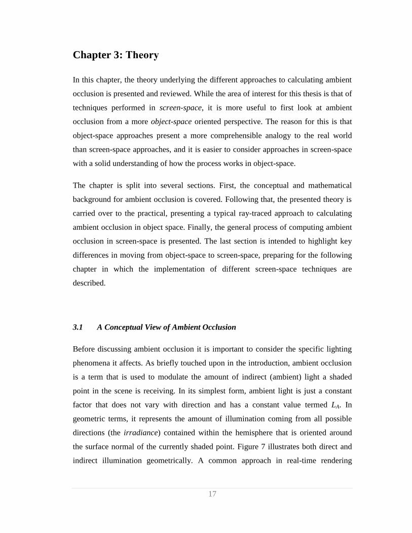
3.1 A Conceptual View of Ambient Occlusion
Before discussing ambient occlusion it is important to consider the specific lighting
phenomena it affects. As briefly touched upon in the introduction, ambient occlusion
is a term that is used to modulate the amount of indirect (ambient) light a shaded
point in the scene is receiving. In its simplest form, ambient light is just a constant
factor that does not vary with direction and has a constant value termed LA. In
geometric terms, it represents the amount of illumination coming from all possible
directions (the irradiance) contained within the hemisphere that is oriented around
the surface normal of the currently shaded point. Figure 7 illustrates both direct and
indirect illumination geometrically. A common approach in real-time rendering
18
scenarios is to simply set the ambient light contribution to the diffuse colour of the
point being shaded and then scale by the ambient light amount represented by LA
(Möller, Haines and Hoffman 2008, 296).
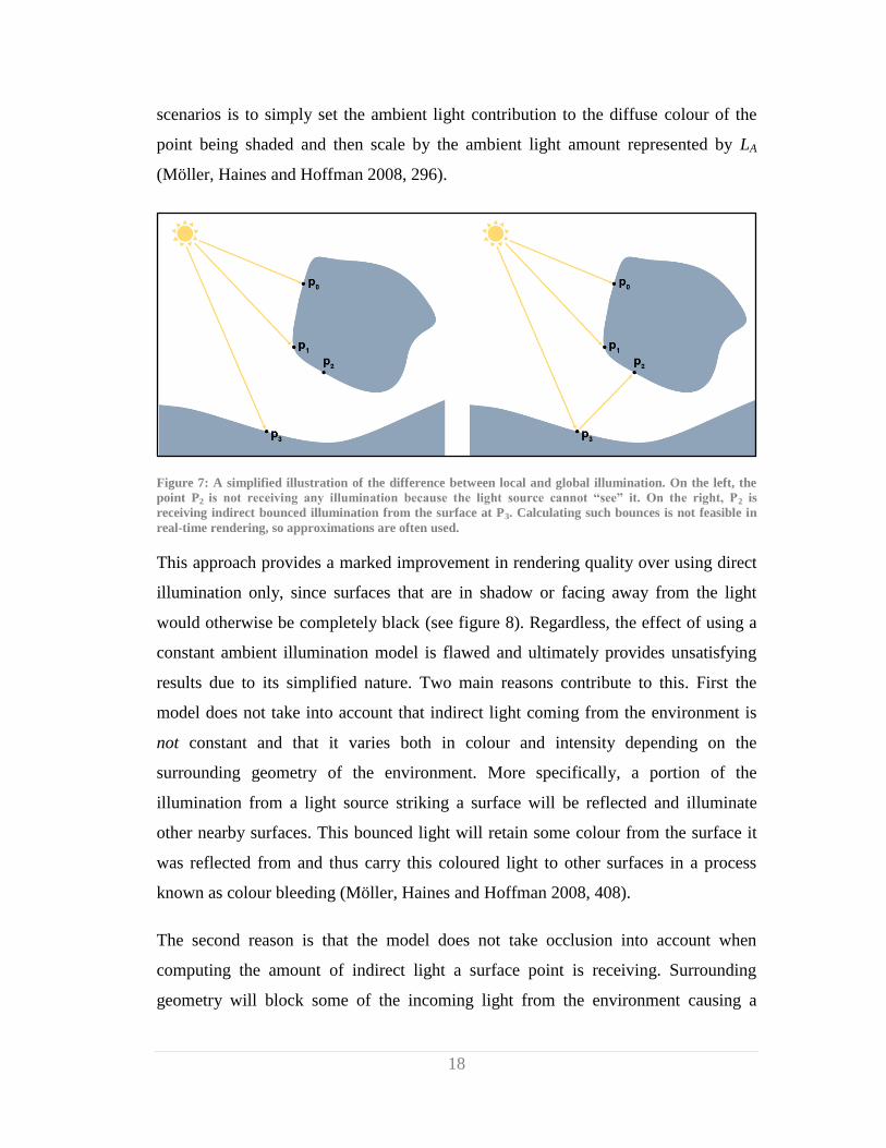
Figure 7: A simplified illustration of the difference between local and global illumination. On the left, the
point P2 is not receiving any illumination because the light source cannot “see” it. On the right, P2 is
receiving indirect bounced illumination from the surface at P3. Calculating such bounces is not feasible in
real-time rendering, so approximations are often used.
This approach provides a marked improvement in rendering quality over using direct
illumination only, since surfaces that are in shadow or facing away from the light
would otherwise be completely black (see figure 8). Regardless, the effect of using a
constant ambient illumination model is flawed and ultimately provides unsatisfying
results due to its simplified nature. Two main reasons contribute to this. First the
model does not take into account that indirect light coming from the environment is
not constant and that it varies both in colour and intensity depending on the
surrounding geometry of the environment. More specifically, a portion of the
illumination from a light source striking a surface will be reflected and illuminate
other nearby surfaces. This bounced light will retain some colour from the surface it
was reflected from and thus carry this coloured light to other surfaces in a process
known as colour bleeding (Möller, Haines and Hoffman 2008, 408).
The second reason is that the model does not take occlusion into account when
computing the amount of indirect light a surface point is receiving. Surrounding
geometry will block some of the incoming light from the environment causing a
19
darkening in the form of soft shadows where there is a lot of surrounding geometry. A
physical approach to modelling this occlusion effect would be to calculate accurate
visibility for all bounces of indirect light. Obviously, this is simply not practical for
real-time purposes and is often forgone in offline rendering scenarios as well when
rendering time is a factor.
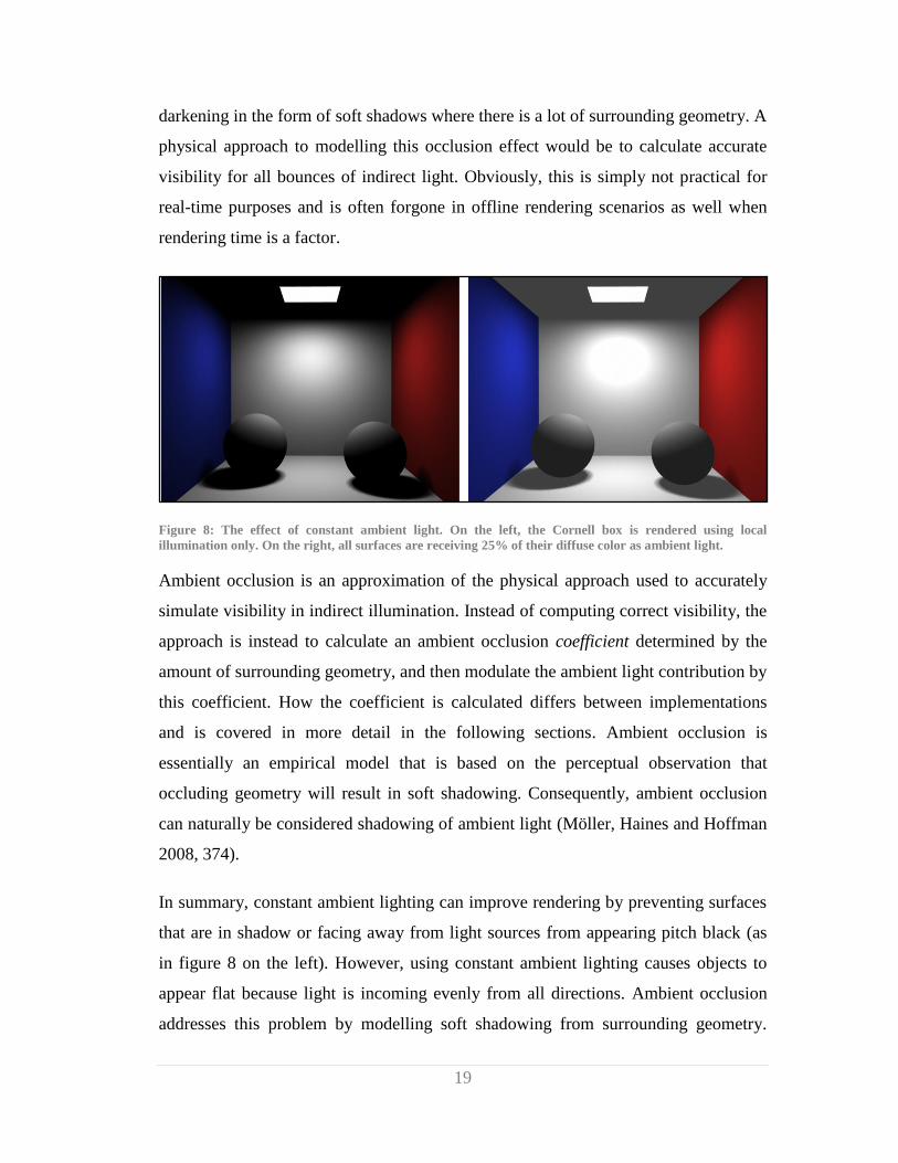
Figure 8: The effect of constant ambient light. On the left, the Cornell box is rendered using local
illumination only. On the right, all surfaces are receiving 25% of their diffuse color as ambient light.
Ambient occlusion is an approximation of the physical approach used to accurately
simulate visibility in indirect illumination. Instead of computing correct visibility, the
approach is instead to calculate an ambient occlusion coefficient determined by the
amount of surrounding geometry, and then modulate the ambient light contribution by
this coefficient. How the coefficient is calculated differs between implementations
and is covered in more detail in the following sections. Ambient occlusion is
essentially an empirical model that is based on the perceptual observation that
occluding geometry will result in soft shadowing. Consequently, ambient occlusion
can naturally be considered shadowing of ambient light (Möller, Haines and Hoffman
2008, 374).
In summary, constant ambient lighting can improve rendering by preventing surfaces
that are in shadow or facing away from light sources from appearing pitch black (as
in figure 8 on the left). However, using constant ambient lighting causes objects to
appear flat because light is incoming evenly from all directions. Ambient occlusion
addresses this problem by modelling soft shadowing from surrounding geometry.

20
Figure 9 illustrates constant ambient lighting with and without ambient occlusion
applied (actually, the constant ambient light seen in figure 9 is just the colour of the
texture, which is equivalent to an ambient light intensity of 1).
Figure 9: The Stanford dragon model rendered using constant ambient lighting alone, and constant
ambient lighting with ambient occlusion applied.
3.2 A Mathematical View of Ambient Occlusion
In this section a more detailed view of ambient occlusion is presented. In the previous
section, constant ambient light was mentioned as the simplest form of indirect
illumination. For the sake of simplicity, only Lambertian diffuse surfaces are
considered in the following, but the equations presented here can be extended to
cover arbitrary bidirectional reflectance distribution functions (BRDFs) (Möller,
Haines and Hoffman 2008, 223). With that in mind, the constant ambient light LA
results in a constant amount of outgoing illumination that does not take the surface
normal or view direction into account. This ambient light can be expressed in the
context of irradiance in the following equation:
( ) ∫
(1)

21
Here, E represents irradiance for the point p with surface normal n, which is the
cosine weighted integral of incoming radiance performed over the hemisphere for
all possible incoming directions (Möller, Haines and Hoffman 2008, 374). As
mentioned, this model does not take visibility or surface orientation into account
which results in the flat appearance seen in figure 9. Extending this equation to
include a simple visibility (occlusion) function ( ) first presented by (Cook and
Torrance 1981) results in the following equation:
( ) ∫ ( )
(2)
The visibility function can vary in complexity. In its simplest form the function
returns a binary value; 0 if the ray representing the incoming direction to the point p
is blocked, and 1 if it is not. As mentioned in the previous section, the ambient
occlusion is actually a coefficient used to modulate the incoming irradiance. This
coefficient is termed and to calculate it, the following equation is derived from (2):
( )
∫ ( )
(3)
The value of the coefficient lies in the range of 0 to 1. If the value is 0, the point
is completely occluded and is receiving no ambient light. If the value is 1, the point is
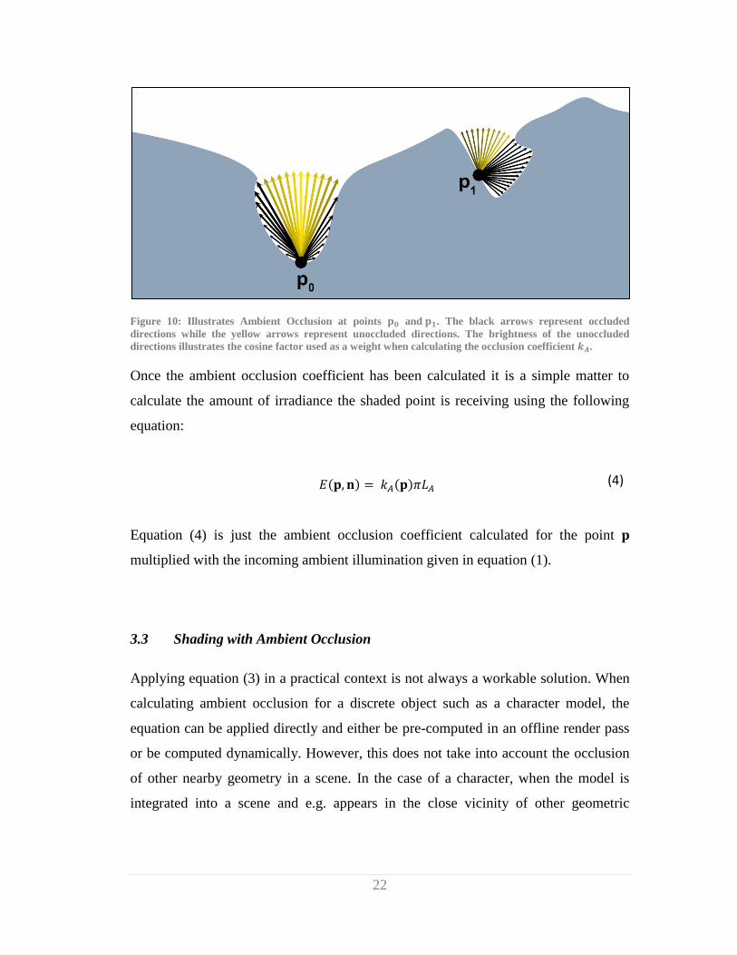
receiving full irradiance which is equivalent to equation (1). Figure 10 illustrates
ambient occlusion geometrically. The black arrows represent the occluded directions
while the yellow arrows represent the unoccluded directions. The brightness of the
yellow arrows illustrates the effect of the cosine factor present in equation (2) and (3).
The visibility function ( ) is weighted by this cosine factor when integrated,
which changes the visibility from a simple binary function to a ranged one. This has
the effect of taking the surface orientation into account when calculating the ambient
occlusion coefficient (Möller, Haines and Hoffman 2008, 375). As a result, is
receiving more irradiance than because the incoming light is centred around the
surface normal, even though their average unoccluded solid angle is similar in size.
22
Figure 10: Illustrates Ambient Occlusion at points and . The black arrows represent occluded
directions while the yellow arrows represent unoccluded directions. The brightness of the unoccluded
directions illustrates the cosine factor used as a weight when calculating the occlusion coefficient .
Once the ambient occlusion coefficient has been calculated it is a simple matter to
calculate the amount of irradiance the shaded point is receiving using the following
equation:
( ) ( ) (4)
Equation (4) is just the ambient occlusion coefficient calculated for the point p
multiplied with the incoming ambient illumination given in equation (1).
3.3 Shading with Ambient Occlusion
Applying equation (3) in a practical context is not always a workable solution. When
calculating ambient occlusion for a discrete object such as a character model, the
equation can be applied directly and either be pre-computed in an offline render pass
or be computed dynamically. However, this does not take into account the occlusion
of other nearby geometry in a scene. In the case of a character, when the model is
integrated into a scene and e.g. appears in the close vicinity of other geometric
23
objects, these objects are not contributing occlusion to the character model and vice
versa.
Moreover, the approach breaks down entirely when applied to a situation of enclosed
geometry such as a room. When evaluating the visibility function ( ) in practice,
the light ray l is checked for intersection with the geometry of the scene to determine
if the incoming light is blocked. In the case of an enclosed space, the visibility
function will always evaluate to zero because the light ray always intersects some
geometry, which has the effect of all points being shaded completely black (assuming
that the point is only receiving ambient illumination). To address this issue, the
visibility function ( ) is usually replaced with a distance mapping
function ( ). This approach called obscurance, first presented by (Zhukov and
Iones 1998), changes the visibility from a binary function to a continuous function of
the distance to the intersection. A user specified maximum distance is used to
limit the range in which intersection is tested for. The distance function then returns a
value of 0 for intersection distances of 0, and 1 at intersection distances of .
Distances beyond are not checked, solving the issue of enclosed geometry in
addition to decreasing the computational cost of computing considerably.
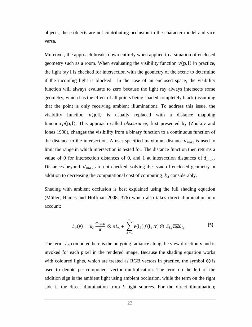
Shading with ambient occlusion is best explained using the full shading equation
(Möller, Haines and Hoffman 2008, 376) which also takes direct illumination into
account:
( ) ∑ ( )
( ) (5)
The term computed here is the outgoing radiance along the view direction v and is
invoked for each pixel in the rendered image. Because the shading equation works
with coloured lights, which are treated as RGB vectors in practice, the symbol is
used to denote per-component vector multiplication. The term on the left of the
addition sign is the ambient light using ambient occlusion, while the term on the right
side is the direct illumination from k light sources. For the direct illumination;
24
( ) is the visibility function which can be evaluated using e.g. shadow mapping;
( ) is the bi-directional reflectance distribution function; is incoming
radiance from light source k; and the last term is the clamped cosine factor of the
angle between the incoming light direction and the surface normal. The factor is
clamped between 0 and 1 to avoid backlighting of surfaces.
Of course, it is the ambient term that is of interest here, and only the term
remains unexplained. The factor is present because the result of integrating a
cosine factor over the hemisphere gives a value of (Möller, Haines and Hoffman
2008, 228). In real-time rendering scenarios, this is usually rolled into the value of
for practical purposes. The value of for Lambertian surfaces is simply the
diffuse colour of the surface. For non-Lambertian surfaces, the value is a blend of the
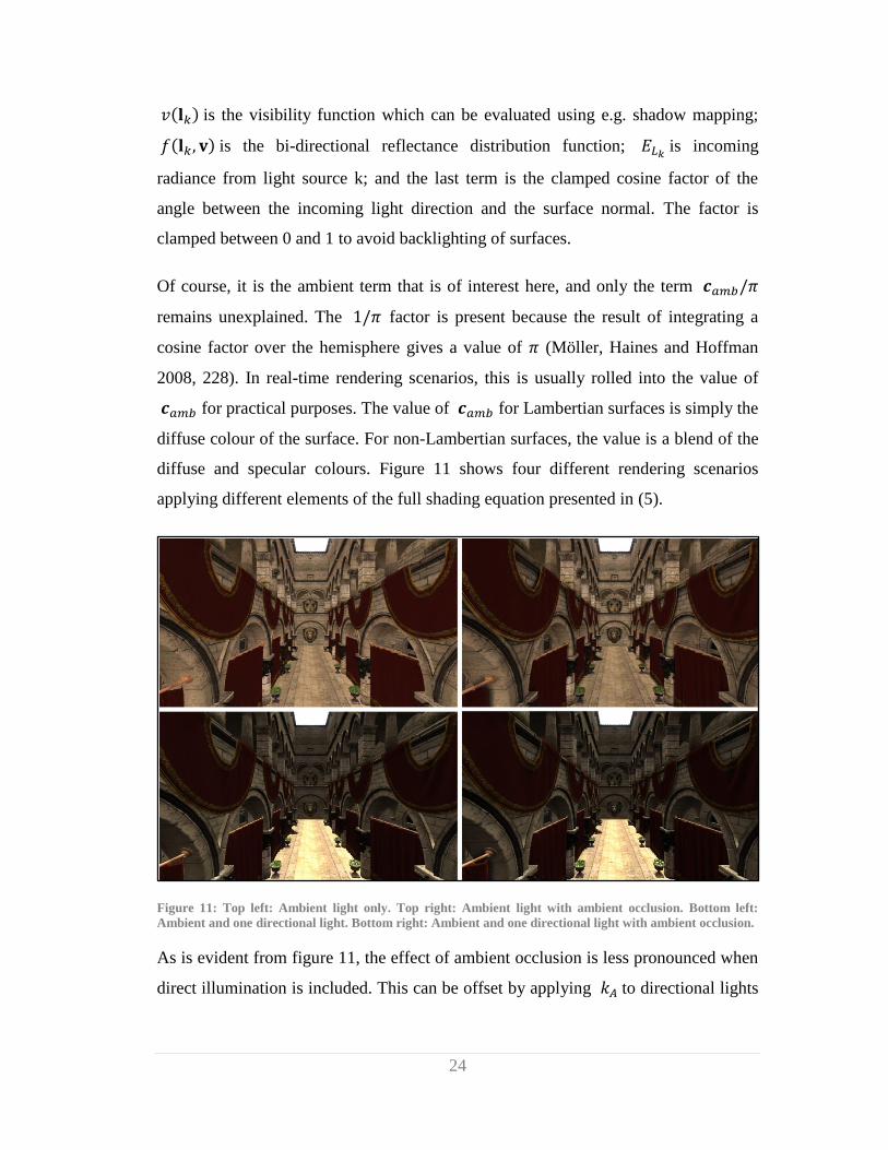
diffuse and specular colours. Figure 11 shows four different rendering scenarios
applying different elements of the full shading equation presented in (5).
Figure 11: Top left: Ambient light only. Top right: Ambient light with ambient occlusion. Bottom left:
Ambient and one directional light. Bottom right: Ambient and one directional light with ambient occlusion.
As is evident from figure 11, the effect of ambient occlusion is less pronounced when
direct illumination is included. This can be offset by applying to directional lights
25
as well, although this is incorrect and will result in darkening of areas where any
direct illumination would prevent such a darkening.
The following two sections take a more pragmatic approach to ambient occlusion
than the mathematical one presented in this section.
3.4 Ambient Occlusion in Object-Space
Calculating ambient occlusion in object-space has in large part already been covered
in the previous section. However, the coverage in the previous section was very
theoretical and the content here serves to provide a more accessible example on how
to calculate ambient occlusion in object space. The material in the previous section
applies both to the scenario of pre-computing ambient occlusion as well as the
scenario of computing it dynamically. From this point on, only dynamic computation
of ambient occlusion is considered.
Because the integral in equation (3) is prohibitively expensive to calculate, a different
approach is usually taken to perform sampling within the hemisphere. A common
approach is to use a Monte Carlo method to generate a uniform distribution of
sampling directions in the hemisphere oriented around the surface normal. Each
generated direction is then treated as a ray for the purpose of testing for intersections
with scene geometry. For complex scenes, this is still computationally expensive, and
a pre-computed acceleration structure is usually employed to prevent intersection
tests with all triangles in the scene. The reason the introduction of the distance
function presented in section 3.3 reduces the computational cost should be evident in
that it further reduces the amount of geometry to perform intersection tests on.
The approach presented in the previous paragraph is a common one for offline
rendering scenarios, but is only useful in real-time rendering for the purpose of pre-
computing static ambient occlusion in a scene. To leverage fully dynamic ambient
26
occlusion in a real-time rendering context, the process has to be moved into screen-
space.
3.5 Ambient Occlusion in Screen-Space
The primary reason the object-space approach presented in section 3.4 is unsuitable
for real-time purposes, is its dependency on the complexity of the scene being
rendered, more specifically the amount of polygons present in the scene. For
contemporary real-time rendering scenarios such as computer games, scene
complexity has long since passed the point where an object-space approach would be
feasible for dynamic computation.
Screen-Space approaches to calculating ambient occlusion are not dependent on the
scene complexity since they are performed in a post-processing pass on the rendered
image. However, screen-space approaches are still based on the same conceptual
basis presented in section 3.1 and therefore still need to access some form of the
scene structure to compute the occlusion factor . This scene structure is present in
the form of the depth-buffer (Z-buffer) of the rendered scene, which contains the
depth of all the pixels that have passed the depth test (i.e. all the visible pixels). In
general terms, screen-space approaches use the information in the Z-buffer as a
limited representation of the full scene geometry to perform the sampling used for
calculating the occlusion factor. In other words, the distance function in section 3.3 is
not performed on the actual scene structure using intersection testing, but rather as a
2D sampling process that relies on the inherent properties of the stored depth-buffer.
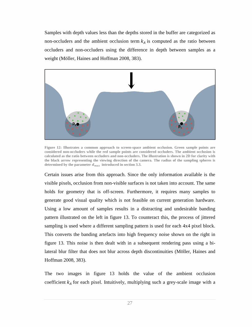
Figure 12 shows a typical example of how the depth buffer can be utilized as a
limited scene structure for performing screen-space ambient occlusion. A certain
amount of points are sampled in the sphere around the shaded point p. The depth of
each sample point is compared to the depth found at the sample pixel in the depth
buffer. If the depth of the sample point is greater than the depth stored in the buffer,
the sample is considered inside the geometry and is categorized as an occluder.
27
Samples with depth values less than the depths stored in the buffer are categorized as
non-occluders and the ambient occlusion term is computed as the ratio between
occluders and non-occluders using the difference in depth between samples as a
weight (Möller, Haines and Hoffman 2008, 383).
Figure 12: Illustrates a common approach to screen-space ambient occlusion. Green sample points are
considered non-occluders while the red sample points are considered occluders. The ambient occlusion is
calculated as the ratio between occluders and non-occluders. The illustration is shown in 2D for clarity with
the black arrow representing the viewing direction of the camera. The radius of the sampling spheres is
determined by the parameter introduced in section 3.3.
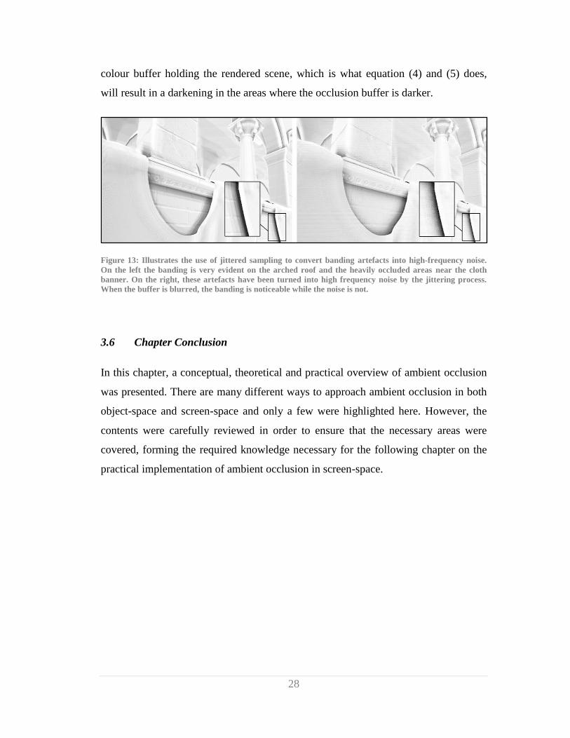
Certain issues arise from this approach. Since the only information available is the
visible pixels, occlusion from non-visible surfaces is not taken into account. The same
holds for geometry that is off-screen. Furthermore, it requires many samples to
generate good visual quality which is not feasible on current generation hardware.
Using a low amount of samples results in a distracting and undesirable banding
pattern illustrated on the left in figure 13. To counteract this, the process of jittered
sampling is used where a different sampling pattern is used for each 4x4 pixel block.
This converts the banding artefacts into high frequency noise shown on the right in
figure 13. This noise is then dealt with in a subsequent rendering pass using a bi-
lateral blur filter that does not blur across depth discontinuities (Möller, Haines and
Hoffman 2008, 383).
The two images in figure 13 holds the value of the ambient occlusion
coefficient for each pixel. Intuitively, multiplying such a grey-scale image with a
28
colour buffer holding the rendered scene, which is what equation (4) and (5) does,
will result in a darkening in the areas where the occlusion buffer is darker.
Figure 13: Illustrates the use of jittered sampling to convert banding artefacts into high-frequency noise.
On the left the banding is very evident on the arched roof and the heavily occluded areas near the cloth
banner. On the right, these artefacts have been turned into high frequency noise by the jittering process.
When the buffer is blurred, the banding is noticeable while the noise is not.
3.6 Chapter Conclusion
In this chapter, a conceptual, theoretical and practical overview of ambient occlusion
was presented. There are many different ways to approach ambient occlusion in both
object-space and screen-space and only a few were highlighted here. However, the
contents were carefully reviewed in order to ensure that the necessary areas were
covered, forming the required knowledge necessary for the following chapter on the
practical implementation of ambient occlusion in screen-space.
29
: Implementation Chapter 4
This chapter deals with the implementation of ambient occlusion in screen-space
necessary for setting up the experiment outlined in chapter 5. The chapter is split into
several different sections dealing with the choice of what occlusion techniques to
implement; the process of implementing a suitable rendering framework into which
the chosen ambient occlusion techniques can be integrated; the actual implementation
of the chosen techniques; and in the last section, some additional implementation
considerations regarding the implementation process as a whole and the ensuing
experiment.
Even though a considerable amount of code was written in implementing the
framework outlined in section 4.2, said section maintains a conceptual style forgoing
any code samples. Conversely, section 4.3 describing the implementation of the
ambient occlusion techniques presents plenty of code samples to illustrate the
process. The presented code is written in Microsoft‟s high level shading language
(HLSL) and prior experience with either this language; the OpenGL shading language
(GLSL); NVidia‟s C for graphics (CG); or even regular C is recommended to get a
comprehensive understanding of the contents.
4.1 Choice of Ambient Occlusion Techniques
The choices regarding which screen-space ambient occlusion techniques to
implement are of course determined by the research question posed and the nature of
the study. Two primary goals for the experimental study were outlined in section 1.2;
the first, to investigate the effect of ambient occlusion on perceived realism; the
second, to assess the effect that physical accuracy of a given technique has on
perceived realism. With these two goals in mind at least two ambient occlusion
techniques that differ in physical accuracy are needed.
30
To cover this need, the two techniques chosen were by (Mittring 2007), described in
section 4.3.1, and by (Filion and McNaughton 2008), described in section 4.3.2; both
were briefly covered in section 2.1. The two were chosen because of a significant
difference in accuracy and apparent quality; although whether this quality difference
is perceivable by naïve (with regards to the experiment purpose and background)
human observers of course remain to be seen.
In addition to these two techniques, a third modified version of the second technique
was also implemented. This technique is more accurate and is described in section
4.3.3. While not strictly needed to address the research question, it was included to
create an experiment condition with a large disparity in algorithm accuracy. For more
details on this, see section 5.3 describing the creation of the experiment stimuli.
4.2 Implementing a Suitable Rendering Framework
The two deciding factors in implementing the rendering framework were
development speed and image quality. The development speed requirement precluded
the use of the more powerful rendering APIs such as DirectX and OpenGL, since they
require a substantial amount of work to get a full rendering context up and running. A
good compromise between development speed and quality was found in Microsoft‟s
game development suite XNA. It provides extensive functionality out of the package
and it is easy and relatively quick to get a rudimentary rendering context running.
Beyond that, XNA provides excellent support for using custom shaders making it a
suitable choice for setting up a rendering framework.
As mentioned, no code is shown in this section but the entirety of the code written
can be found on the accompanying CD. The remainder of this section serves as a
conceptual overview of the rendering framework implemented allowing for the
integration of the different ambient occlusion techniques to follow.
31
In section 2.1 it was established that screen-space ambient occlusion techniques
requires a depth buffer for sampling the scene structure and that some approaches
require the surface normals of shaded pixels as well. Regarding the techniques
described in this chapter, the first only uses the depth information while the last two
use the surface normals as well. The basic requirement of having access to both scene
depth and surface normals had a significant bearing on the manner in which the
rendering framework was implemented.
Because screen-space ambient occlusion techniques (and screen-space techniques in
general) are carried out in a post-processing pass, i.e. they are performed after the
scene has already been rendered; accessing the scene depth and especially the surface
normal is not a trivial matter. An additional issue is presented due to the way the
underlying graphics API (in this case DirectX) stores the depth of the rendered pixels.
The depth is stored in a non-linear depth buffer with more precision allocated to scene
elements that are closer to the camera. This works well for sorting objects which is
the primary purpose of the depth buffer, but this non-linearity is not ideal for
techniques such as ambient occlusion. This creates the additional requirement of
having access to a linear version of the depth buffer with equal precision across the
entire range of the scene.
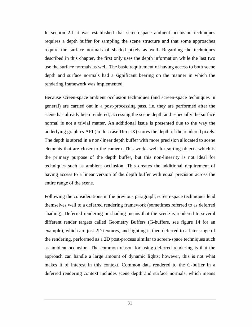
Following the considerations in the previous paragraph, screen-space techniques lend
themselves well to a deferred rendering framework (sometimes referred to as deferred
shading). Deferred rendering or shading means that the scene is rendered to several
different render targets called Geometry Buffers (G-buffers, see figure 14 for an
example), which are just 2D textures, and lighting is then deferred to a later stage of
the rendering, performed as a 2D post-process similar to screen-space techniques such
as ambient occlusion. The common reason for using deferred rendering is that the
approach can handle a large amount of dynamic lights; however, this is not what
makes it of interest in this context. Common data rendered to the G-buffer in a
deferred rendering context includes scene depth and surface normals, which means
32
that in a deferred rendering context, this data is readily available for all post-
processing operations including screen-space ambient occlusion.
For these reasons, a deferred rendering framework was implemented in XNA which
could easily support several different screen-space ambient occlusion techniques.
Figure 14 shows the basic flow of the deferred rendering framework. A few details
such as ambient lighting and high-dynamic range processing have been left out of the
figure for the sake of clarity.
Figure 14: Illustrates the rendering flow of the deferred rendering framework. The G-buffers are rendered
first and consists of the diffuse colour, surface normals, and scene depth. Lighting is then performed using
the stored normals and depth. Modulating the diffuse colours with the lighting creates the composite image
shown at the bottom.
The important point to illustrate here is that once the final colour image is rendered
(shown on the bottom), the diffuse, normal and depth information is retained and is
free to be utilised in a post-processing pass, be it colour grading, depth of field,
ambient occlusion, or some other post-processing technique.
33
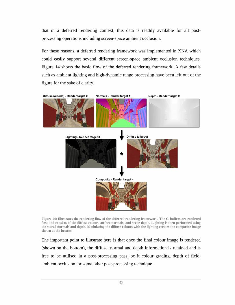
The format of the 2D render targets holding the stored information of the G-buffers is
important, and should be carefully chosen for the desired output. Most importantly,
the depth buffer needs at least 16 bits to properly represent the depth of the scene.
Using lower bit depths results in banding artefacts in the lighting and more
importantly, unusable ambient occlusion results due to insufficient precision. Table 1
illustrates the render targets used for the basic deferred rendering setup.
Table 1: The three render targets used for the basic deferred rendering setup. Two four channel 32 bit
targets were used for the diffuse, specular and normal data. A single channel 32 bit render target was used
to store the linear depth.
Target / Channel Red Green Blue Alpha
Render target 0
8 bits/channel Red Diffuse Green Diffuse Blue Diffuse
Specular Intensity
Render target 1
8 bits/channel Normal X Normal Y Normal Z
Specular Power
Render target 2
Single Channel Depth (32 bits)
A few additional render targets were used in addition to these fundamental ones. The
most important ones are listed in table 2.
Table 2: Additional render targets used: Render targets 3 and 4 uses 16 bits per channel to enable high
dynamic range lighting. Only one 8 bit channel is needed for the ambient occlusion coefficient.
Target / Channel Red Green Blue Alpha
Render target 3
16 bits/channel Red Light Green Light Blue Light
Specular Light
(monochromatic)
Render target 4
16 bits/channel
Red Final Colour
Green Final Colour
Blue Final Colour
Unused
Render target 5
8 bits / channel Unused Unused Unused
Ambient Occlusion Coefficient
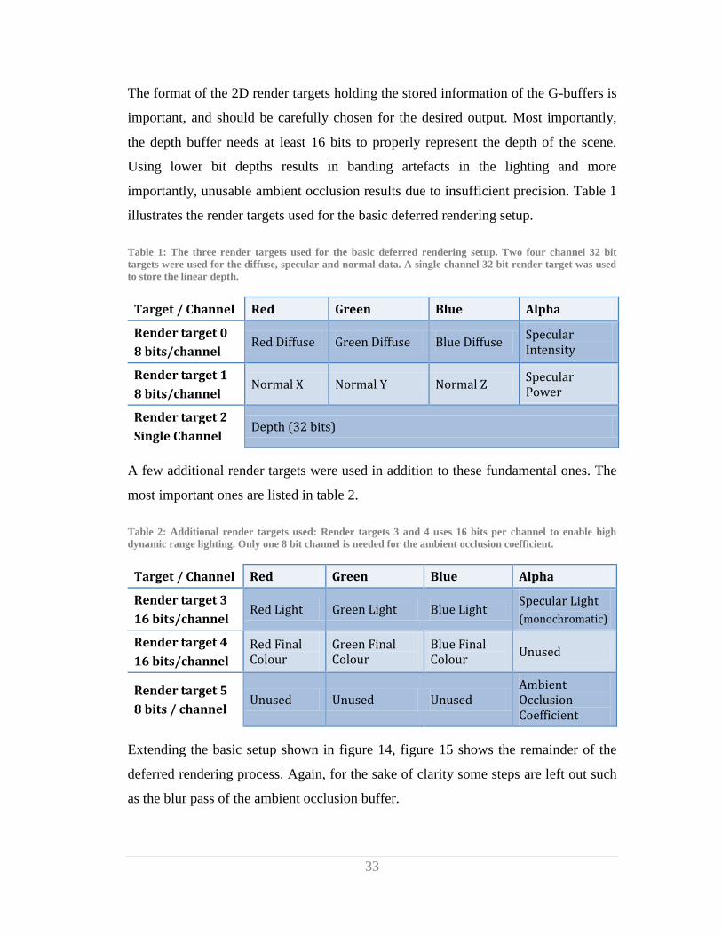
Extending the basic setup shown in figure 14, figure 15 shows the remainder of the
deferred rendering process. Again, for the sake of clarity some steps are left out such
as the blur pass of the ambient occlusion buffer.
34
Figure 15: The final steps of the deferred rendering process. The last operation resulting in the final image
is a tone mapping operator, mapping the high dynamic range values to be displayed on a low dynamic
range device. When not using high dynamic range lighting, very bright areas are clipped to white as seen in
the middle image. Note how render target 4 is reused several times. The multiplication of the ambient
occlusion buffer is actually taking place in the compositing step of figure 14 while the tone mapping is
operating on a copy of render target 4. Sampling from, and writing to, the same render target in one pass is
not allowed.
The choice of implementing the rendering framework in the manner presented here
allowed for easy integration of multiple screen-space ambient occlusion techniques.
The following section outlines the implementation of the three techniques used in the
experimental study.
35
4.3 Implementing the Ambient Occlusion Techniques
For the sake of brevity, the different techniques described here have been given
specific names. For the first two techniques, the names given are that of the respective
companies from which the techniques originated, Crytek (Mittring 2007) and
Blizzard (Filion and McNaughton 2008). The third technique is an extension of the
Blizzard technique and is named Ray-Marching, the reasons for which are outlined in
section 4.3.3.
Code comments are not included here since the comments are usually covered in the
text, but all three ambient occlusion shaders can be viewed in full, including
comments, in the appendix or on the accompanying CD.
The contents of the following three sections can be difficult to follow and the
following conventions should aid in understanding. Each ambient occlusion technique
is performed in a full-screen post-processing pass, which is essentially a large loop
iterating through each pixel of the image being processed. When performing ambient
occlusion, the image being processed is of course the stored depth buffer. For each
pixel, another loop structure is utilised to generate samples around this pixel used in
accumulating the ambient occlusion. An important point to remember is that each
pixel in the depth buffer represents the world space position of the surface point that
was found closest to the camera. Any samples generated around this point also
represent positions in world space. However, the positions of these samples also
correspond to positions stored in the depth buffer, but the position in the depth buffer
will usually have a different depth than the sample position. Computing the difference
between the depth of the sample pixel and the depth of the pixel position, we can
figure out if the current sample position is in front or behind the point stored in the
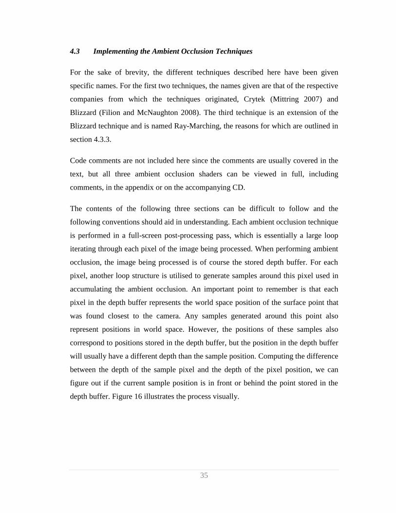
depth buffer. Figure 16 illustrates the process visually.
36
Figure 16: Illustrates the sampling and depth comparison process used in the ambient occlusion pass. The
process is shown in 2D for clarity and the black arrow represents the camera viewing direction. The point P
is the current pixel being processed. The sample point S0 is the current sample point and the point S1 is the
surface position found in the depth buffer at the position of S0. The white arrow illustrates the depth
difference between the two samples. Point P0 illustrates a scenario where the sample is found in front of the
point. Point P1 illustrates a scenario where the sample is found behind.
The text presented in the following three sections covering the three different ambient
occlusion techniques share a common factor; they all describe the operation that takes
place on a single pixel of the depth buffer (not counting the samples around the pixel
for calculating the ambient occlusion). So the contents of each section describe a
single iteration of the large loop mentioned in the previous paragraph, and for all
techniques the process is then repeated for the total amount of pixels in the image.
4.3.1 Crytek Technique
The approach presented in this section is an adaption of the technique used in the
computer game Crysis (Crytek 2007). More specifically, it is an adaption of the code
presented in the book ShaderX7 (Kajalin 2009) by the original creator of the
technique. By admission of the author himself, the code presented in the book is not
the same as the production code used in the release version of Crysis, and some lines
were changed or modified for the implementation here as well. As a consequence, the
technique is not exactly the same as seen in Crysis; however, the end result is
reasonably close and more importantly, it exhibits the same artefacts which makes it
37
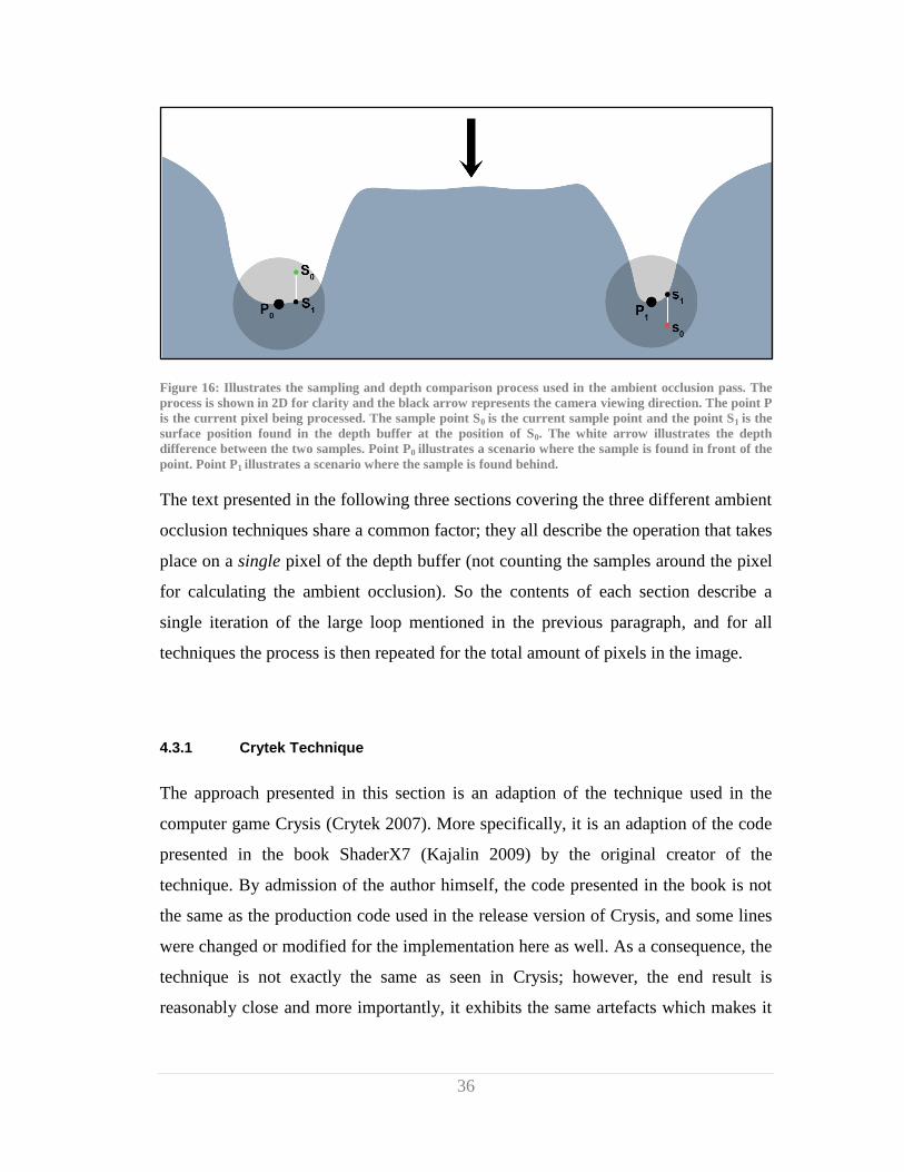
less accurate than the Blizzard and Ray-Marching techniques. Figure 17 shows the
three main artefacts that make the Crytek approach the least accurate technique. The
function for computing ambient occlusion using this technique can be viewed in full
in appendix A.
Figure 17: An example buffer of the Crytek ambient occlusion technique. Three major artefacts are present
here; the edge highlighting (A); the pillars occluding (darkening) part of the wall behind which are too far
away (B); and the occlusion of planar surfaces which should be unoccluded (C). The buffer shown here is
not blurred.
4.3.1.1 Initialising Steps
The first step of the Crytek technique as well as the other two techniques surprisingly
have nothing to do with ambient occlusion per se, but is a necessary step to
circumvent certain limitations in the way the graphics card works. Essentially, all
three ambient occlusion techniques presented need a random vector sampled from a
texture; but using the unmodified texture coordinates of the pixel being processed to
sample the random vector results in the distracting noise pattern on the left of figure
18. What is needed is a non-uniform sampling strategy for retrieving the vector, and
this is handled by the following line of code:
38
float2 rotationTC = screenTC * screenSize / 4.0f;
The variable screenTC holds the texture coordinates of the current pixel while the
screenSize variable holds the width and height of the current resolution. As is evident,
the modified texture coordinates stored in rotationTC is scaled by one quarter of the
screen resolution. The resulting modified (tiled) texture coordinates are used for
retrieving the random vector from a pre-defined texture map handled by the following
line of code:
float3 vRotation = 2 * tex2D(sRandVectSampler, rotationTC).rgb - 1;
The variable sRandVectSampler holds the texture map containing the random vectors
(see figure 18 middle) from which a vector is retrieved and stored in vRotation. Since
the vector is stored in the range of 0 to 1, the vector is transformed to the correct -1 to
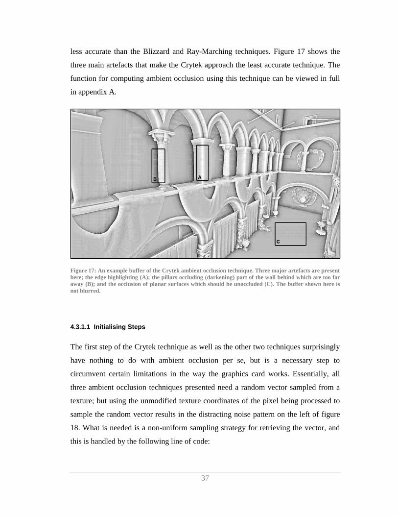
1 range. Using the modified texture coordinates to non-uniformly sample the random
vector is a very important step for all three techniques, and figure 18 on the right
shows the result of using the modified coordinates.
Figure 18: The result of tiling the texture coordinates used to sample the random vectors. On the left no
tiling is used, while on the right tiling is used. The texture holding the random vectors is shown in the
middle. The XYZ components of the vectors are stored in the RGB channels of the texture causing the
coloured noise pattern.
The actual use of the random vector and the reason for this process will be explained
shortly. Following the random vector sampling, the depth value at the current pixel is
read from the depth buffer and stored in the variable fSceneDepthP and the occlusion
factor is initialized to 0:
float fSceneDepthP = tex2D(sSceneDepthSampler, screenTC).r;

39
float fAccessibility = 0;
Note that in this technique the occlusion factor is actually called accessibility.
Interestingly, this is more accurate terminology since the value being accumulated for
each pixel is actually the accessibility and not the occlusion. One way to look at it is
to consider that an accessibility value of 0 corresponds to a completely occluded
point; while a value of 1 means that the point is completely unoccluded. In other
words, accessibility is the inverse of occlusion.
4.3.1.2 Generating Samples
The next step is to sample a specified number of points around the current pixel
position and accumulate the accessibility or occlusion factor, depending on how you
look at it. For the Crytek technique this process is handled in a multi-nested loop
shown in the following code sample:
for(int i = 0 ; i < (nSamplesNum/8) ; i++)
for(int x = -1 ; x <= 1 ; x += 2)
for(int y = -1 ; y <= 1 ; y += 2)
for(int z = -1 ; z <= 1 ; z += 2)
Until otherwise noted, the code samples in the following text are performed inside
these loops. The variable nSamplesNum is set to the desired number of samples to
generate around the current pixel position. The three inner loops go through the
corners of the unit cube which is used in the following line of code to generate
different offset vectors:
float3 vOffset = normalize(float3(x, y, z)) * offsetScale;
The variable offsetScale represents the variable presented in section 3.3. This
variable controls the radius of the sphere that samples are being generated in, and
therefore the distance to which surfaces are taken into account for occlusion. As they
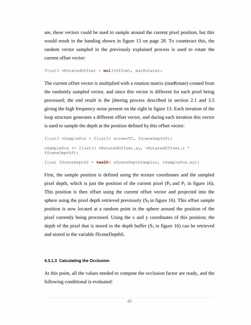
40
are, these vectors could be used to sample around the current pixel position, but this
would result in the banding shown in figure 13 on page 28. To counteract this, the
random vector sampled in the previously explained process is used to rotate the
current offset vector:
float3 vRotatedOffset = mul(vOffset, matRotate);
The current offset vector is multiplied with a rotation matrix (matRotate) created from
the randomly sampled vector, and since this vector is different for each pixel being
processed; the end result is the jittering process described in section 2.1 and 3.5
giving the high frequency noise present on the right in figure 13. Each iteration of the
loop structure generates a different offset vector, and during each iteration this vector
is used to sample the depth at the position defined by this offset vector:
float3 vSamplePos = float3( screenTC, fSceneDepthP);
vSamplePos += float3( vRotatedOffset.xy, vRotatedOffset.z *
fSceneDepthP);
float fSceneDepthS = tex2D( sSceneDepthSampler, vSamplePos.xy);
First, the sample position is defined using the texture coordinates and the sampled
pixel depth, which is just the position of the current pixel (P0 and P1 in figure 16).
This position is then offset using the current offset vector and projected into the
sphere using the pixel depth retrieved previously (S0 in figure 16). This offset sample
position is now located at a random point in the sphere around the position of the
pixel currently being processed. Using the x and y coordinates of this position; the
depth of the pixel that is stored in the depth buffer (S1 in figure 16) can be retrieved
and stored in the variable fSceneDepthS.
4.3.1.3 Calculating the Occlusion
At this point, all the values needed to compute the occlusion factor are ready, and the
following conditional is evaluated:
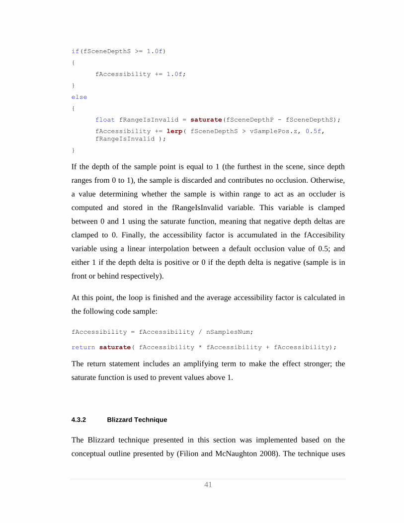
41
if(fSceneDepthS >= 1.0f)
{
fAccessibility += 1.0f;
}
else
{
float fRangeIsInvalid = saturate(fSceneDepthP - fSceneDepthS);
fAccessibility += lerp( fSceneDepthS > vSamplePos.z, 0.5f,
fRangeIsInvalid );
}
If the depth of the sample point is equal to 1 (the furthest in the scene, since depth
ranges from 0 to 1), the sample is discarded and contributes no occlusion. Otherwise,
a value determining whether the sample is within range to act as an occluder is
computed and stored in the fRangeIsInvalid variable. This variable is clamped
between 0 and 1 using the saturate function, meaning that negative depth deltas are
clamped to 0. Finally, the accessibility factor is accumulated in the fAccesibility
variable using a linear interpolation between a default occlusion value of 0.5; and
either 1 if the depth delta is positive or 0 if the depth delta is negative (sample is in
front or behind respectively).
At this point, the loop is finished and the average accessibility factor is calculated in
the following code sample:
fAccessibility = fAccessibility / nSamplesNum;
return saturate( fAccessibility * fAccessibility + fAccessibility);
The return statement includes an amplifying term to make the effect stronger; the
saturate function is used to prevent values above 1.
4.3.2 Blizzard Technique
The Blizzard technique presented in this section was implemented based on the
conceptual outline presented by (Filion and McNaughton 2008). The technique uses
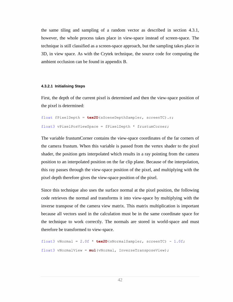
42
the same tiling and sampling of a random vector as described in section 4.3.1,
however, the whole process takes place in view-space instead of screen-space. The
technique is still classified as a screen-space approach, but the sampling takes place in
3D, in view space. As with the Crytek technique, the source code for computing the
ambient occlusion can be found in appendix B.
4.3.2.1 Initialising Steps
First, the depth of the current pixel is determined and then the view-space position of
the pixel is determined:
float fPixelDepth = tex2D(sSceneDepthSampler, screenTC).r;
float3 vPixelPosViewSpace = fPixelDepth * frustumCorner;
The variable frustumCorner contains the view-space coordinates of the far corners of
the camera frustum. When this variable is passed from the vertex shader to the pixel
shader, the position gets interpolated which results in a ray pointing from the camera
position to an interpolated position on the far clip plane. Because of the interpolation,
this ray passes through the view-space position of the pixel, and multiplying with the
pixel depth therefore gives the view-space position of the pixel.
Since this technique also uses the surface normal at the pixel position, the following
code retrieves the normal and transforms it into view-space by multiplying with the
inverse transpose of the camera view matrix. This matrix multiplication is important
because all vectors used in the calculation must be in the same coordinate space for
the technique to work correctly. The normals are stored in world-space and must
therefore be transformed to view-space.
float3 vNormal = 2.0f * tex2D(sNormalSampler, screenTC) - 1.0f;
float3 vNormalView = mul(vNormal, InverseTransposeView);
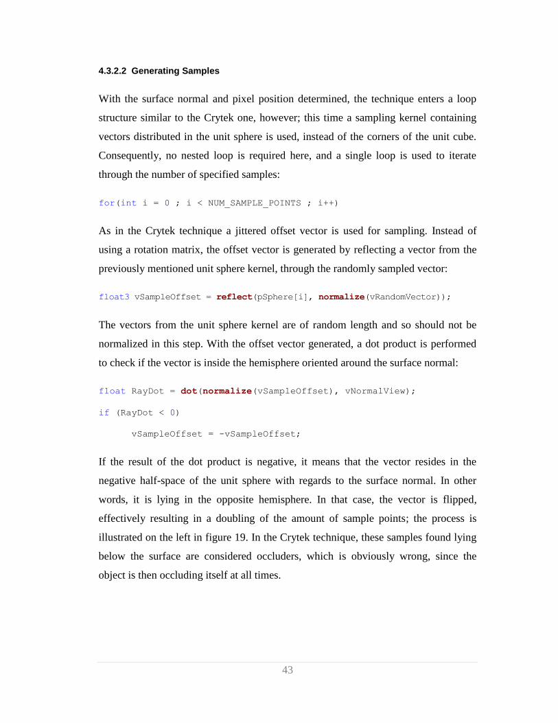
43
4.3.2.2 Generating Samples
With the surface normal and pixel position determined, the technique enters a loop
structure similar to the Crytek one, however; this time a sampling kernel containing
vectors distributed in the unit sphere is used, instead of the corners of the unit cube.
Consequently, no nested loop is required here, and a single loop is used to iterate
through the number of specified samples:
for(int i = 0 ; i < NUM_SAMPLE_POINTS ; i++)
As in the Crytek technique a jittered offset vector is used for sampling. Instead of
using a rotation matrix, the offset vector is generated by reflecting a vector from the
previously mentioned unit sphere kernel, through the randomly sampled vector:
float3 vSampleOffset = reflect(pSphere[i], normalize(vRandomVector));
The vectors from the unit sphere kernel are of random length and so should not be
normalized in this step. With the offset vector generated, a dot product is performed
to check if the vector is inside the hemisphere oriented around the surface normal:
float RayDot = dot(normalize(vSampleOffset), vNormalView);
if (RayDot < 0)
vSampleOffset = -vSampleOffset;
If the result of the dot product is negative, it means that the vector resides in the
negative half-space of the unit sphere with regards to the surface normal. In other
words, it is lying in the opposite hemisphere. In that case, the vector is flipped,
effectively resulting in a doubling of the amount of sample points; the process is
illustrated on the left in figure 19. In the Crytek technique, these samples found lying
below the surface are considered occluders, which is obviously wrong, since the
object is then occluding itself at all times.
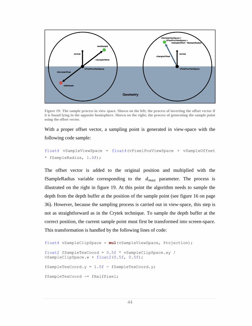
44
Figure 19: The sample process in view space. Shown on the left; the process of inverting the offset vector if
it is found lying in the opposite hemisphere. Shown on the right; the process of generating the sample point
using the offset vector.
With a proper offset vector, a sampling point is generated in view-space with the
following code sample:
float4 vSampleViewSpace = float4(vPixelPosViewSpace + vSampleOffset
* fSampleRadius, 1.0f);
The offset vector is added to the original position and multiplied with the
fSampleRadius variable corresponding to the parameter. The process is
illustrated on the right in figure 19. At this point the algorithm needs to sample the
depth from the depth buffer at the position of the sample point (see figure 16 on page
36). However, because the sampling process is carried out in view-space, this step is
not as straightforward as in the Crytek technique. To sample the depth buffer at the
correct position, the current sample point must first be transformed into screen-space.
This transformation is handled by the following lines of code:
float4 vSampleClipSpace = mul(vSampleViewSpace, Projection);
float2 fSampleTexCoord = 0.5f * vSampleClipSpace.xy /
vSampleClipSpace.w + float2(0.5f, 0.5f);
fSampleTexCoord.y = 1.0f - fSampleTexCoord.y;
fSampleTexCoord -= fHalfPixel;
45
First, the sample is transformed to clip space using the perspective projection matrix.
Then the sample texture coordinates are calculated by doing a homogenous divide
and transforming into the 0 to 1 range. Finally, the coordinates are flipped around the
y-axis and the texture coordinates are aligned with the pixel coordinates. This process
results in texture coordinates that can be used to sample the depth from the depth
buffer:
float fSampleDepth = tex2D(sSceneDepthSampler, fSampleTexCoord).r;
4.3.2.3 Calculating the Occlusion
At this point, the occlusion factor can be calculated and stored in the fResult variable.
Note that fResult is initialised to 0 which indicates full occlusion. In this technique,
the occlusion is accumulated using a variable called fOcclusionFactor, however; like
in the Crytek technique, what is actually being accumulated is the accessibility factor.
The difference is only semantic, but it is mentioned to prevent confusion of the terms.
To compute the occlusion factor, the depth delta between the pixel and sample depth
is calculated:
float fDepthDelta = max(fSampleDepth - fPixelDepth , 0);
The max function returns the largest value of the two parameters, so if the depth delta
is negative a value of 0 is returned. This depth delta is then used to calculate the
occlusion factor using the following two lines of code:
float fOcclusionFactor = fDistanceScale * fDepthDelta;
fOcclusionFactor = 1.0f / (1.0f + fOcclusionFactor *
fOcclusionFactor);
The fDistanceScale holds the full depth of the scene (the distance from the near clip
plane to the far clip plane). Because the technique uses linear depth stored in the 0 to
1 range, the depth delta is converted to scene unit scale by multiplying with the
distance scale. This is a necessary step because the occlusion function in this

46
technique includes a quadratic attenuation of the distance to control the amount of
occlusion. Without the distance scale, the attenuation is much too strong, resulting in
no occlusion being calculated anywhere in the scene, i.e. a completely white
occlusion buffer. Following the distance scale, the occlusion is calculated using the
quadratic attenuation and the following conditional is evaluated to accumulate the
occlusion factor:
if(fDepthDelta < fFullOccThreshold || fDepthDelta > fNoOccThreshold)
{
fResult += 1.0f;
}
else
{
fOcclusionFactor = pow(fOcclusionFactor, fOcclusionPow);
fResult += fOcclusionFactor;
}
Two artistic variables (fFullOccThreshold and fNoOccThreshold) are used to limit
the occlusion within a certain threshold. Since screen-space ambient occlusion is
empirical and not physical, such artistic variables are commonly used to adjust the
effect for a desired look. If the depth delta falls outside the range between these two
variables, the point is considered completely unoccluded, i.e. it has an accessibility of
1. An exponential variable fOcclusionPow is used to further control the strength of
the occlusion. As with the Crytek technique, the return value of the occlusion
function is the mean of the accumulated occlusion across all samples:
return fResult / NUM_SAMPLE_POINTS;
For an example of the ambient occlusion buffer generated using this technique, see
section 4.3.4.
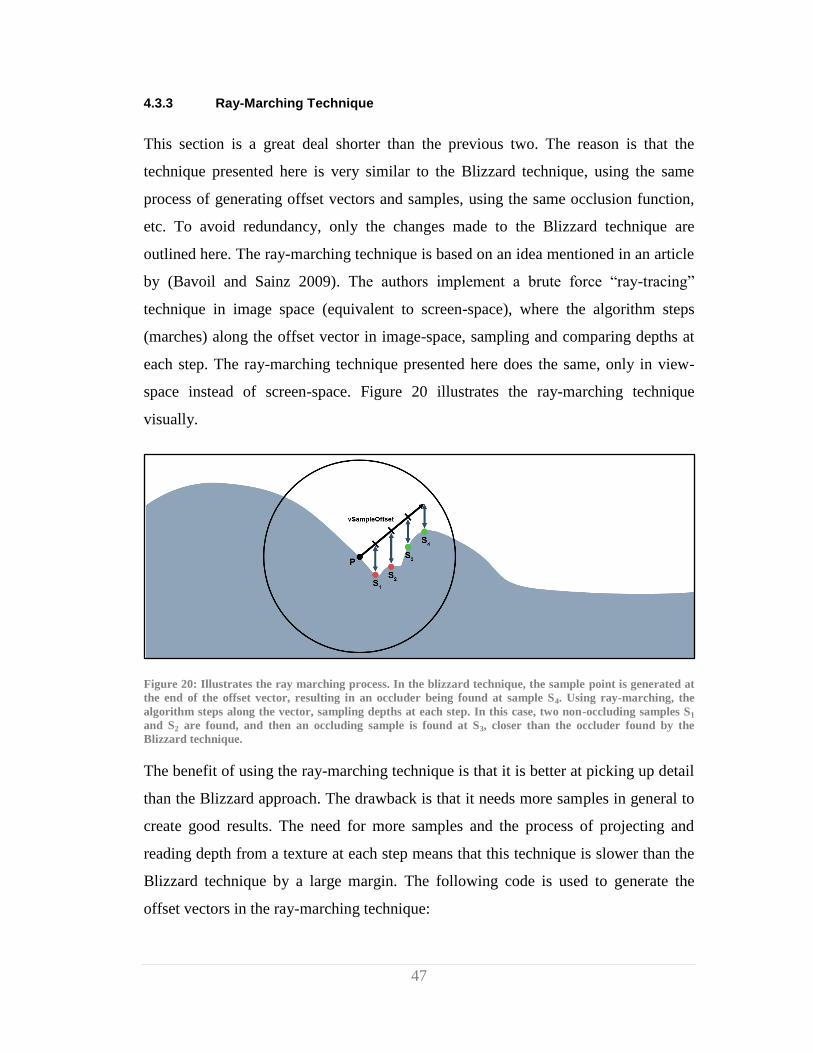
47
4.3.3 Ray-Marching Technique
This section is a great deal shorter than the previous two. The reason is that the
technique presented here is very similar to the Blizzard technique, using the same
process of generating offset vectors and samples, using the same occlusion function,
etc. To avoid redundancy, only the changes made to the Blizzard technique are
outlined here. The ray-marching technique is based on an idea mentioned in an article
by (Bavoil and Sainz 2009). The authors implement a brute force “ray-tracing”
technique in image space (equivalent to screen-space), where the algorithm steps
(marches) along the offset vector in image-space, sampling and comparing depths at
each step. The ray-marching technique presented here does the same, only in view-
space instead of screen-space. Figure 20 illustrates the ray-marching technique
visually.
Figure 20: Illustrates the ray marching process. In the blizzard technique, the sample point is generated at
the end of the offset vector, resulting in an occluder being found at sample S4. Using ray-marching, the
algorithm steps along the vector, sampling depths at each step. In this case, two non-occluding samples S1
and S2 are found, and then an occluding sample is found at S3, closer than the occluder found by the
Blizzard technique.
The benefit of using the ray-marching technique is that it is better at picking up detail
than the Blizzard approach. The drawback is that it needs more samples in general to
create good results. The need for more samples and the process of projecting and
reading depth from a texture at each step means that this technique is slower than the
Blizzard technique by a large margin. The following code is used to generate the
offset vectors in the ray-marching technique:
48
float3 vStep = (1.0f / NUM_STEPS) * vSampleOffset * fSampleRadius;
Assuming that NUM_STEPS is set to 4, this generates an offset vector that is one
quarter length of the original offset vector. The same transformation to screen-space
and sampling of the depth buffer as in section 4.3.2 is performed and the depth delta
is computed. If the following conditional evaluates to true, it means that no occluder
was found at this step and the algorithm continues to the next step along the offset
vector:
if(fDepthDelta < fFullOccThreshold)
The rest of the process is identical to the Blizzard technique, using the same function
to accumulate the occlusion factor. The code for this technique can be found in
appendix C. For an example of the occlusion buffer generated by this technique, see
the following section.
4.3.4 Techniques Comparison and Discussion
This section reviews the three different techniques presented in the previous three
sections, and discuss the differences between them. To begin with, figure 21 shows
three ambient occlusion buffers generated using the three different techniques. The
buffers are also included on the CD in full size for closer examination. As is evident
from comparing the images in figure 21, the blizzard technique exhibits less problems
with self-occlusion compared to the Crytek technique, particularly noticeable on the
floor and the walls. The Blizzard technique also exhibits better detail than the Crytek
one, most noticeable in the form of more intense occlusion in heavily occluded areas
such as between the lower curtains and the arches. This is largely due to the better
distribution of sample points in the Blizzard technique. While the Blizzard technique
still exhibits edge highlighting to some degree, it is much more noticeable in the
Crytek technique because of the relative brightness difference caused by the self-
occlusion. When applied to a textured and lit scene, the edge highlighting is generally
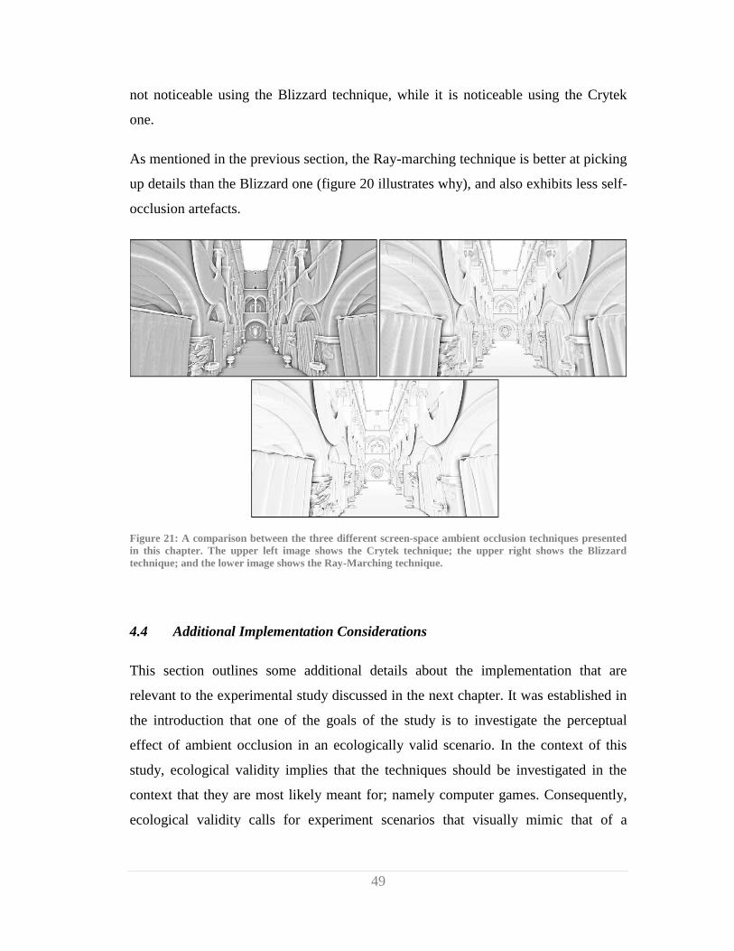
49
not noticeable using the Blizzard technique, while it is noticeable using the Crytek
one.
As mentioned in the previous section, the Ray-marching technique is better at picking
up details than the Blizzard one (figure 20 illustrates why), and also exhibits less self-
occlusion artefacts.
Figure 21: A comparison between the three different screen-space ambient occlusion techniques presented
in this chapter. The upper left image shows the Crytek technique; the upper right shows the Blizzard
technique; and the lower image shows the Ray-Marching technique.
4.4 Additional Implementation Considerations
This section outlines some additional details about the implementation that are
relevant to the experimental study discussed in the next chapter. It was established in
the introduction that one of the goals of the study is to investigate the perceptual
effect of ambient occlusion in an ecologically valid scenario. In the context of this
study, ecological validity implies that the techniques should be investigated in the
context that they are most likely meant for; namely computer games. Consequently,
ecological validity calls for experiment scenarios that visually mimic that of a

50
computer game in visual complexity. This not only impacts the design of the stimuli
discussed in section 5.3, but also adds additional requirements to the rendering
framework. To increase the ecological validity of the experiment stimuli, several
additional features were added to the rendering framework including normal
mapping, irradiance environment mapping, as well as support for rendering skyboxes.
The high dynamic range lighting was implemented using a third party tone mapping
class while the bi-lateral blurring of the occlusion buffers were handled using code
adapted from (Bavoil and Sainz 2009).
These additional features combined with directional lighting and standard texture
mapping allows for the creation of complex visual stimuli, mimicking the visual
complexity of modern computer games. It is important to note that the goal of
ecological validity in this study pertains primarily to the visual complexity of the still
images presented. Obviously, the most ecologically valid scenario for performing a
perceptual study examining these occlusion techniques would be an interactive setting
such as a computer game, but the experimental approach in this study uses still
images. The reasons for why are outlined in section 5.2.
All stimuli sets used in the experiment can be viewed in section 5.3 in the following
chapter, in the appendix, as well as on the CD in full resolution.
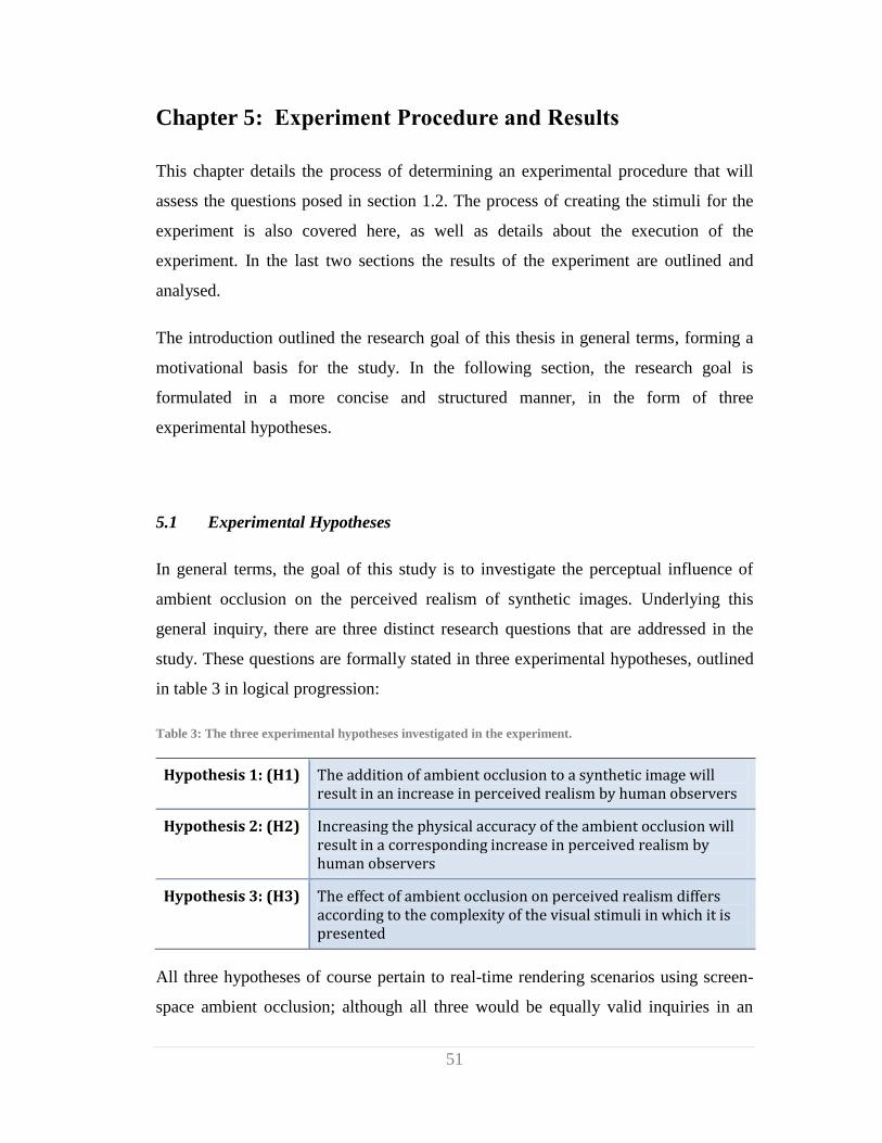
51
: Experiment Procedure and Results Chapter 5
This chapter details the process of determining an experimental procedure that will
assess the questions posed in section 1.2. The process of creating the stimuli for the
experiment is also covered here, as well as details about the execution of the
experiment. In the last two sections the results of the experiment are outlined and
analysed.
The introduction outlined the research goal of this thesis in general terms, forming a
motivational basis for the study. In the following section, the research goal is
formulated in a more concise and structured manner, in the form of three
experimental hypotheses.
5.1 Experimental Hypotheses
In general terms, the goal of this study is to investigate the perceptual influence of
ambient occlusion on the perceived realism of synthetic images. Underlying this
general inquiry, there are three distinct research questions that are addressed in the
study. These questions are formally stated in three experimental hypotheses, outlined
in table 3 in logical progression:
Table 3: The three experimental hypotheses investigated in the experiment.
Hypothesis 1: (H1) The addition of ambient occlusion to a synthetic image will result in an increase in perceived realism by human observers
Hypothesis 2: (H2) Increasing the physical accuracy of the ambient occlusion will result in a corresponding increase in perceived realism by human observers
Hypothesis 3: (H3) The effect of ambient occlusion on perceived realism differs according to the complexity of the visual stimuli in which it is presented
All three hypotheses of course pertain to real-time rendering scenarios using screen-
space ambient occlusion; although all three would be equally valid inquiries in an
52
offline rendering scenario using e.g. ray-traced ambient occlusion. The null
hypothesis for H1 is that the addition of ambient occlusion will not increase the
perceived realism; for H2, the null hypothesis is that increasing accuracy will not
increase perceived realism; finally, for H3 the null hypothesis is that ecological
validity has no bearing on ambient occlusion‟s effect on perceived realism.
5.2 Experiment Procedure
This section outlines the considerations behind the design of the experimental
procedure used to investigate the experimental hypotheses outlined in the previous
section. Several existing approaches to measuring visual realism in synthetic images
were discussed in section 2.2 and this section builds on the observations made there.
A determining factor in this study is that it should possess a high level of ecological
validity. Arguably, the most ecologically valid scenario would be to have experiment
participants navigate a virtual environment freely, allowing them to experience the
environment with and without ambient occlusion, as well as with occlusion
techniques of different physical accuracy; all without allowing for any direct
comparison. Participants would then perform a subjective evaluation of which
scenario they found the most visually realistic. Unfortunately, this approach provides
no guarantee that subjects perceive the same imagery, with the most extreme case
being that their subjective evaluation are based on entirely different factors.
Comparing results in such cases would be fruitless as they would possess no internal
validity.
A compromise is needed between ecological and internal validity so that the results
can be interpreted and generalised in a meaningful context. An acceptable
compromise is to follow a no-reference approach using visually complex image pairs
as stimuli. (Yu, et al. 2009) use five second videos as stimuli and using videos was
initially considered for this experiment procedure as well. However, the cited
experiment allows for direct and continuous comparison between the stimuli videos.
53
The no-reference approach adopted here does not allow for such direct comparison
and as a consequence, the use of videos was ruled out. The reasoning behind this
decision was that the temporal span of even very short videos would be too much for
participants to retain and process without the possibility of direct comparison.
Using the approach of comparing image pairs, the stimuli can be presented in a more
controlled albeit less ecologically valid manner, ensuring consistency between results.
The choice of experimental approach in this study is thus very similar to the ones
carried out by (Jimenez, Sundstedt and Gutierrez 2009) and (Sundstedt, et al. 2007).
In more descriptive terms, experiment participants should be subjected to stimuli in
the form of image pairs designed specifically for investigating the hypotheses
outlined in the previous section; and then be tasked with performing a subjective
evaluation following each image pair. By adopting this approach, stimuli that only
change along one dimension can be designed providing a more controlled scenario
with only one independent variable; either the presence or absence of ambient
occlusion; or changing physical accuracy of the occlusion technique used. As a
consequence, any patterns observed in the dependent variable (the perceived realism)
should be due to these changing factors alone (Bartz, et al. 2008). This puts an
emphasis on the importance of carefully designed stimuli pairs, which is the subject
of the next section. One remaining crucially important part of the experiment
procedure is the formulation of instructions for the experiment participants.
The approach outlined thus far requires participants to make a simple evaluation
between two images, resulting in a binary choice. However, the manner in which
participants are prompted to evaluate the images can exert great influence on
participants‟ responses. The reason for this is that human perception is not driven by
stimuli alone, but also by cognitive constraints such as goals and expectations
(Palmer 1999, 13-14). Phrasing the instructions is thus a delicate balance; attempting
to elicit the kind of responses from participants that will apply to the research in
question, but without priming them and contaminating the results in the process.
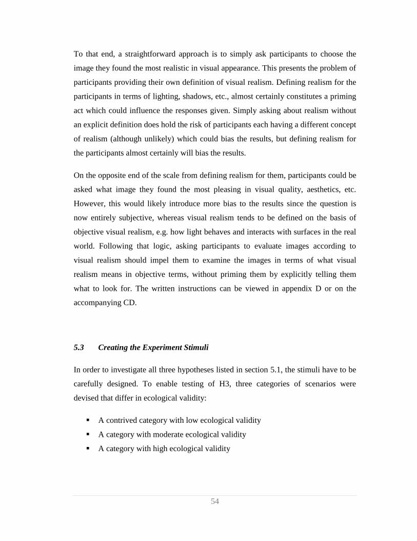
54
To that end, a straightforward approach is to simply ask participants to choose the
image they found the most realistic in visual appearance. This presents the problem of
participants providing their own definition of visual realism. Defining realism for the
participants in terms of lighting, shadows, etc., almost certainly constitutes a priming
act which could influence the responses given. Simply asking about realism without
an explicit definition does hold the risk of participants each having a different concept
of realism (although unlikely) which could bias the results, but defining realism for
the participants almost certainly will bias the results.
On the opposite end of the scale from defining realism for them, participants could be
asked what image they found the most pleasing in visual quality, aesthetics, etc.
However, this would likely introduce more bias to the results since the question is
now entirely subjective, whereas visual realism tends to be defined on the basis of
objective visual realism, e.g. how light behaves and interacts with surfaces in the real
world. Following that logic, asking participants to evaluate images according to
visual realism should impel them to examine the images in terms of what visual
realism means in objective terms, without priming them by explicitly telling them
what to look for. The written instructions can be viewed in appendix D or on the
accompanying CD.
5.3 Creating the Experiment Stimuli
In order to investigate all three hypotheses listed in section 5.1, the stimuli have to be
carefully designed. To enable testing of H3, three categories of scenarios were
devised that differ in ecological validity:
A contrived category with low ecological validity
A category with moderate ecological validity
A category with high ecological validity

55
Within each category, stimuli sets were created to enable investigation of H1 and H2.
The following subsections detail the three categories and the stimuli sets that were
created for them. To distinguish between the images of the stimuli sets, the technique
names outlined in section 4.3 are used. In addition, the names are suffixed with a
number representing the amount of samples used, e.g. Blizzard24 means that the
Blizzard technique from section 4.3.2 was used with a sample frequency of 24. All
the stimuli can and should be viewed on the CD in the original resolution; which is
1280x720. Enlarged (but not full sized) versions of the stimuli pairs can also be
viewed in appendix E-K for convenience. Each figure in the following sections refers
to the corresponding appendix section.
Because screen-space approaches to ambient occlusion are empirical and not
physical, there is no right way to configure the techniques. As evident from the
implementation details for each technique implemented, they all have different
variables that can be adjusted and consequently change the appearance of the
occlusion. Considerate effort was made to match the different techniques in
appearance without compensating for any artefacts intrinsic to the technique. For
example, no attempt was made to match the edge highlighting and self-occlusion of
the Crytek technique when adjusting the Blizzard technique, but the sampling radius
of both techniques were adjusted so that they would roughly affect the same area.
5.3.1 Low Ecological Validity
This category represents a contrived scenario that uses only a single object, with no
illumination except for a constant ambient contribution of 1.
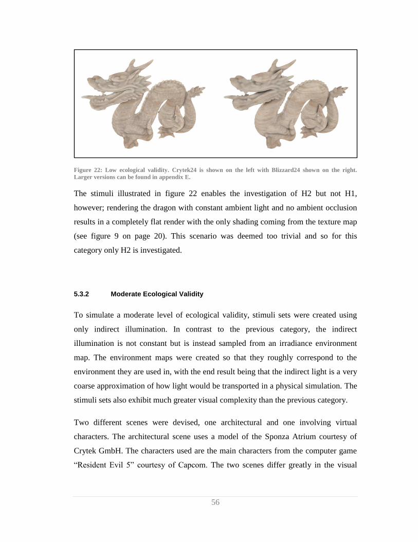
56
Figure 22: Low ecological validity. Crytek24 is shown on the left with Blizzard24 shown on the right.
Larger versions can be found in appendix E.
The stimuli illustrated in figure 22 enables the investigation of H2 but not H1,
however; rendering the dragon with constant ambient light and no ambient occlusion
results in a completely flat render with the only shading coming from the texture map
(see figure 9 on page 20). This scenario was deemed too trivial and so for this
category only H2 is investigated.
5.3.2 Moderate Ecological Validity
To simulate a moderate level of ecological validity, stimuli sets were created using
only indirect illumination. In contrast to the previous category, the indirect
illumination is not constant but is instead sampled from an irradiance environment
map. The environment maps were created so that they roughly correspond to the
environment they are used in, with the end result being that the indirect light is a very
coarse approximation of how light would be transported in a physical simulation. The
stimuli sets also exhibit much greater visual complexity than the previous category.
Two different scenes were devised, one architectural and one involving virtual
characters. The architectural scene uses a model of the Sponza Atrium courtesy of
Crytek GmbH. The characters used are the main characters from the computer game
“Resident Evil 5” courtesy of Capcom. The two scenes differ greatly in the visual

57
dominance of the ambient occlusion. For the architectural scene, the ambient
occlusion is a moderately dominant feature as illustrated in figure 23.
Figure 23: Moderate ecological validity. No ambient occlusion is shown on the left with Blizzard24 shown
on the right. Larger versions can be found in appendix F.
Figure 23 enables the investigation of H1. To investigate H2 in the context of
moderate ecological validity, a second image pair was created shown in figure 24.
Figure 24: Moderate ecological validity. Crytek24 is shown on the left with Blizzard24 shown on the right.
Larger versions can be found in appendix G.
For the characters, the ambient occlusion is much less dominant, primarily due to less
spatial area showing the ambient occlusion, but also because the characters have a
certain amount of occlusion pre-computed into their texture maps. Such pre-
computation is a common approach in real-time rendering and is the primary reason
for including these characters into the stimuli sets. Only one stimuli pair was created
for the characters in this category and is shown in figure 25. This stimuli pair was
included to investigate a large disparity in objective occlusion quality, evident by the
techniques and sample quantities used.
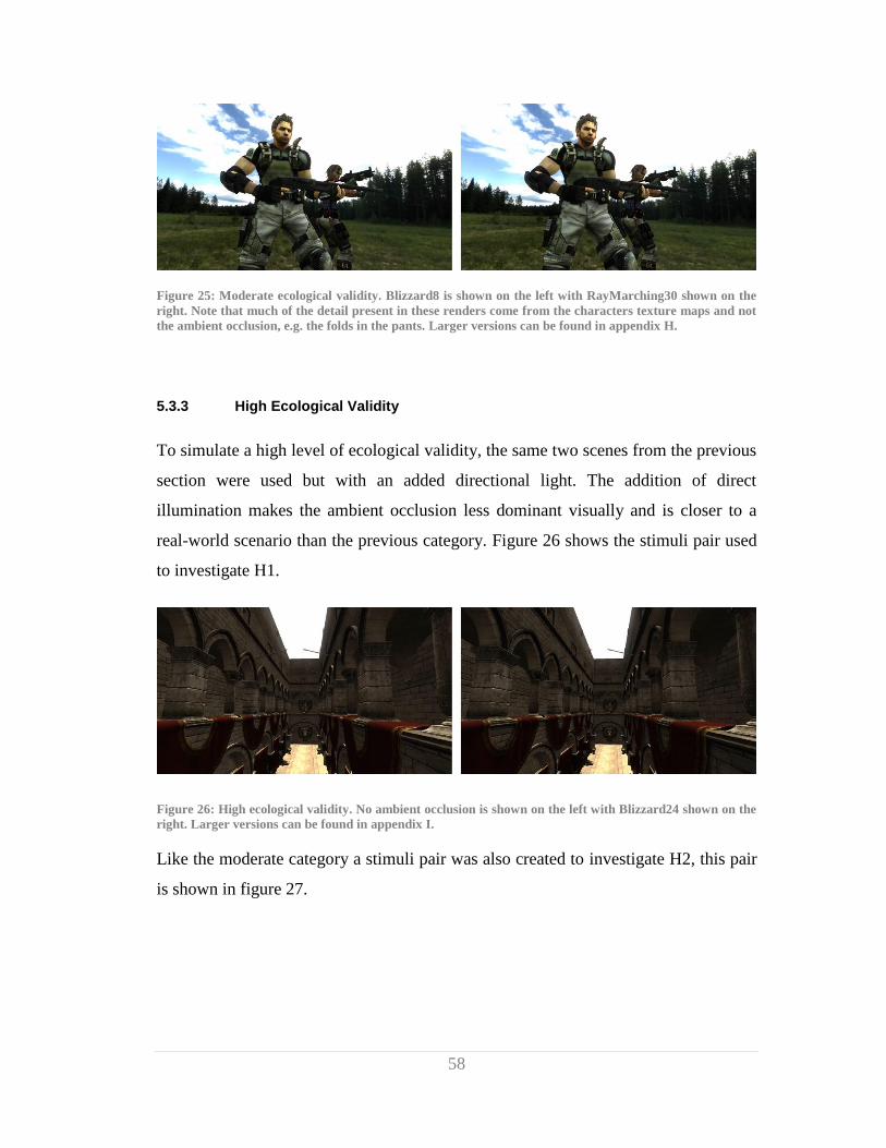
58
Figure 25: Moderate ecological validity. Blizzard8 is shown on the left with RayMarching30 shown on the
right. Note that much of the detail present in these renders come from the characters texture maps and not
the ambient occlusion, e.g. the folds in the pants. Larger versions can be found in appendix H.
5.3.3 High Ecological Validity
To simulate a high level of ecological validity, the same two scenes from the previous
section were used but with an added directional light. The addition of direct
illumination makes the ambient occlusion less dominant visually and is closer to a
real-world scenario than the previous category. Figure 26 shows the stimuli pair used
to investigate H1.
Figure 26: High ecological validity. No ambient occlusion is shown on the left with Blizzard24 shown on the
right. Larger versions can be found in appendix I.
Like the moderate category a stimuli pair was also created to investigate H2, this pair
is shown in figure 27.
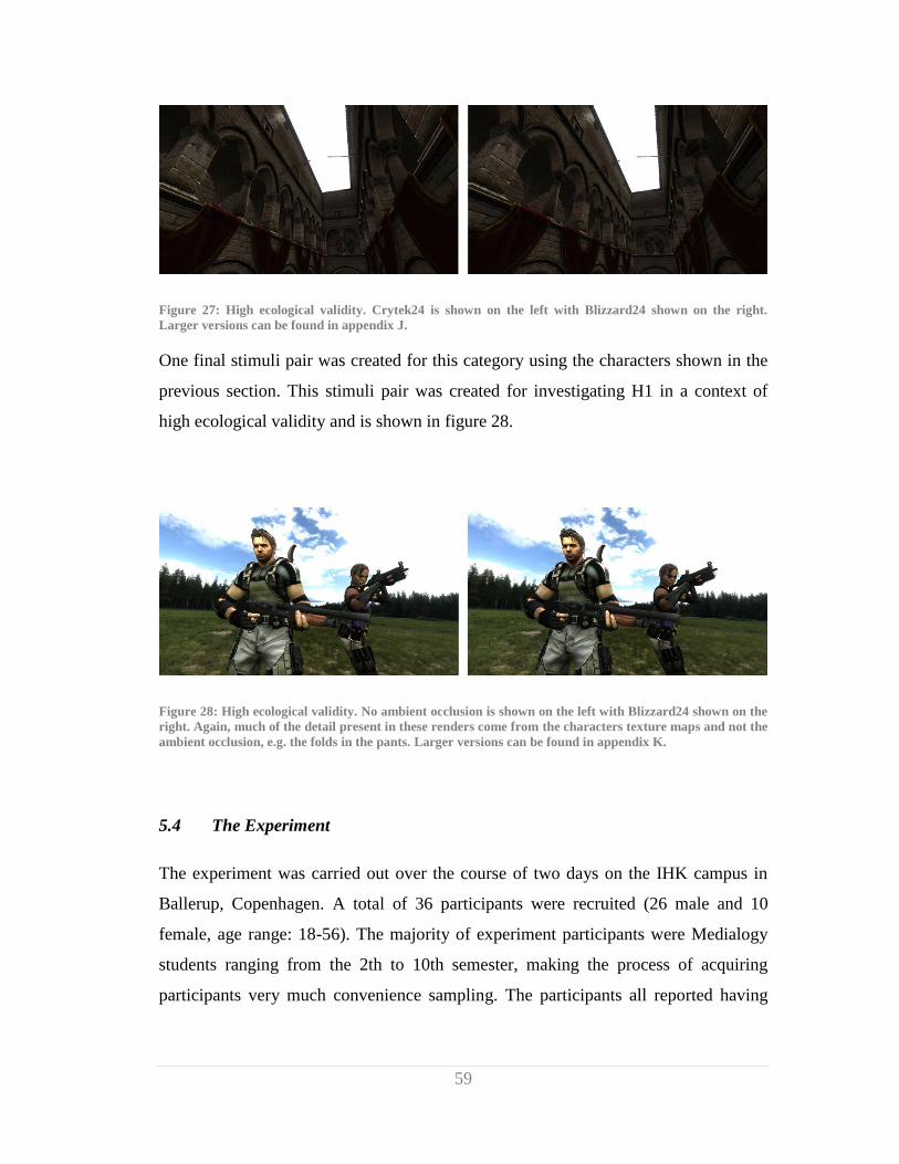
59
Figure 27: High ecological validity. Crytek24 is shown on the left with Blizzard24 shown on the right.
Larger versions can be found in appendix J.
One final stimuli pair was created for this category using the characters shown in the
previous section. This stimuli pair was created for investigating H1 in a context of
high ecological validity and is shown in figure 28.
Figure 28: High ecological validity. No ambient occlusion is shown on the left with Blizzard24 shown on the
right. Again, much of the detail present in these renders come from the characters texture maps and not the
ambient occlusion, e.g. the folds in the pants. Larger versions can be found in appendix K.
5.4 The Experiment
The experiment was carried out over the course of two days on the IHK campus in
Ballerup, Copenhagen. A total of 36 participants were recruited (26 male and 10
female, age range: 18-56). The majority of experiment participants were Medialogy
students ranging from the 2th to 10th semester, making the process of acquiring
participants very much convenience sampling. The participants all reported having
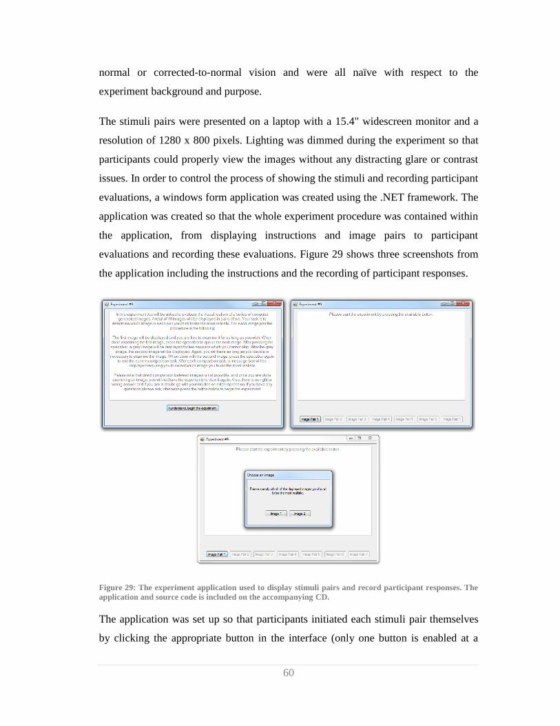
60
normal or corrected-to-normal vision and were all naïve with respect to the
experiment background and purpose.
The stimuli pairs were presented on a laptop with a 15.4" widescreen monitor and a
resolution of 1280 x 800 pixels. Lighting was dimmed during the experiment so that
participants could properly view the images without any distracting glare or contrast
issues. In order to control the process of showing the stimuli and recording participant
evaluations, a windows form application was created using the .NET framework. The
application was created so that the whole experiment procedure was contained within
the application, from displaying instructions and image pairs to participant
evaluations and recording these evaluations. Figure 29 shows three screenshots from
the application including the instructions and the recording of participant responses.
Figure 29: The experiment application used to display stimuli pairs and record participant responses. The
application and source code is included on the accompanying CD.
The application was set up so that participants initiated each stimuli pair themselves
by clicking the appropriate button in the interface (only one button is enabled at a
61
time), thus allowing participants to control the pace of the experiment themselves. By
clicking the available image pair button, the first image of the current pair is shown
and participants are given as much time as they deem necessary to examine the
image. When done, participants were instructed to press the space bar to move on to
the second image of the stimuli pair. In between the images, a mid-grey image was
shown to prevent any direct comparison and to indicate the onset of the next image.
Participants also controlled the time taken to examine the second image, and were
then instructed to press the spacebar when done to initiate the evaluation step.
After each image pair, participants were asked to select which image looked the most
realistic in a message box shown in the bottom of figure 29. Participants proceeded in
this manner through all image pairs until done with the experiment.
Since the experiment procedure is a within-subject design, where each participant are
subjected to all conditions (image pairs), the order of presentation is important.
Simply presenting the same order to all participants could create order bias and
randomising the order does not guarantee that the same condition will not appear e.g.
first in several experiment runs. Instead, a Latin Square design was utilised to create
different orders for each participant. Since there are a total of 7 conditions, a 7th order
latin square was used to assign the conditions. However, since there are two images in
each condition, the order within conditions should also be taken into account. To
account for this, after 7 experiments have been run, the internal orders of the
conditions are reversed and the latin square is run again. Once 14 experiments have
been performed, a new latin square is generated for subsequent experiments. This
process was handled internally and transparently in the experiment application.
Results were recorded automatically by the application and saved to a csv file for
processing in Excel. The next section presents the results that were obtained from the
experiment procedure.

62
5.5 The Results
In this section the results of the experiment are presented as is, with no analysis or
discussion. The raw results of the csv file can be found on the CD. The results are
presented here in order of the categories presented in section 5.3.
5.5.4 Low Ecological Validity Results
The only condition present in this category was the Stanford dragon (figure 22). In
response to the stimuli, participants were evenly divided with 18 votes recorded in
favour of the Crytek technique and 18 in favour of the Blizzard technique.
5.5.5 Moderate Ecological Validity Results
In the moderate category there were three conditions for evaluation. For the occlusion
versus no-occlusion scenario (figure 23 page 57), 14 votes were recorded in favour of
the no-occlusion scenario with 22 recorded in favour of the occlusion scenario. For
the Crytek versus Blizzard scenario (figure 24 page 57), 11 votes were recorded in
favour or the Crytek technique with 25 votes recorded in favour of the Blizzard one.
For the characters (figure 25 page 58), the results were 16 votes for the Blizzard
technique with 20 for the Ray-Marching technique.
5.5.6 High Ecological Validity Results
Three conditions were evaluated in the high category. For the no-occlusion versus
occlusion scenario (figure 26 page 58), the results were 11 for no-occlusion and 25
for the Blizzard technique. For the Crytek versus Blizzard condition (figure 27 page
59), the results were evenly divided with 18 in favour of the Crytek technique, and 18
in favour of the Blizzard technique. For the last condition with the characters (figure
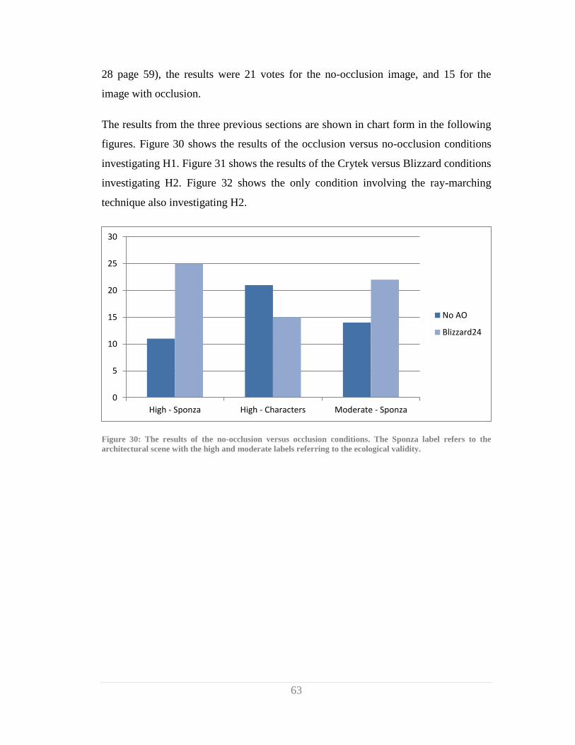
63
28 page 59), the results were 21 votes for the no-occlusion image, and 15 for the
image with occlusion.
The results from the three previous sections are shown in chart form in the following
figures. Figure 30 shows the results of the occlusion versus no-occlusion conditions
investigating H1. Figure 31 shows the results of the Crytek versus Blizzard conditions
investigating H2. Figure 32 shows the only condition involving the ray-marching
technique also investigating H2.
Figure 30: The results of the no-occlusion versus occlusion conditions. The Sponza label refers to the
architectural scene with the high and moderate labels referring to the ecological validity.
0
5
10
15
20
25
30
High - Sponza High - Characters Moderate - Sponza
No AO
Blizzard24

64
Figure 31: The results of the Crytek versus Blizzard conditions. The Sponza label refers to the architectural
scene with the high and moderate labels referring to the ecological validity.
Figure 32: The results of the Blizzard versus Ray-Marching condition.
5.6 Statistical Analysis
A non-parametric technique called a Chi-Square was used to determine if there were
any significance to the results, or if the distributions were what to expect by random
chance (Jimenez, Sundstedt and Gutierrez 2009) (Sundstedt, et al. 2007). For each
condition, the results were compared to an expected 18/18 distribution, indicating no
0
5
10
15
20
25
30
Low - Dragon High - Sponza Moderate - Sponza
Crytek24
Blizzard24
0
5
10
15
20
25
Moderate - Characters
Blizzard8
Ray-Marching30
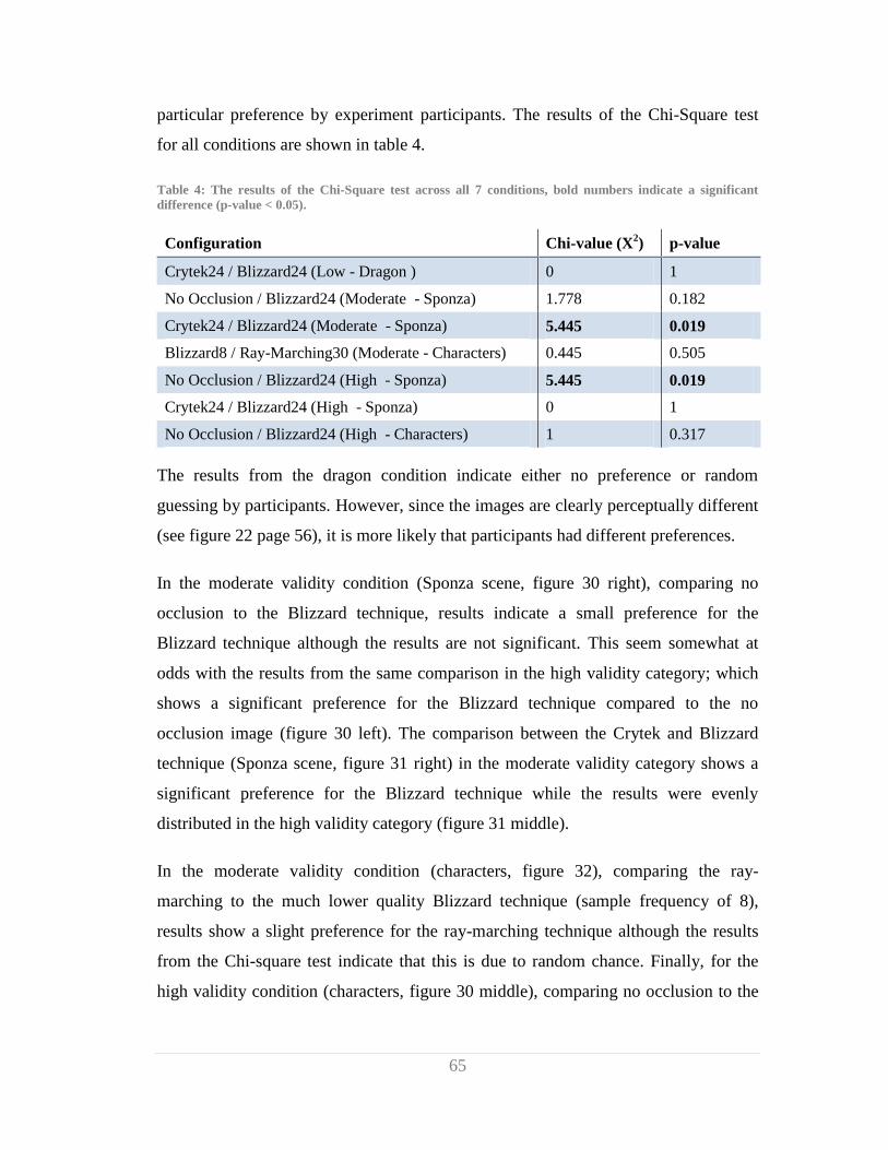
65
particular preference by experiment participants. The results of the Chi-Square test
for all conditions are shown in table 4.
Table 4: The results of the Chi-Square test across all 7 conditions, bold numbers indicate a significant
difference (p-value < 0.05).
Configuration Chi-value (X2) p-value
Crytek24 / Blizzard24 (Low - Dragon ) 0 1
No Occlusion / Blizzard24 (Moderate - Sponza) 1.778 0.182
Crytek24 / Blizzard24 (Moderate - Sponza) 5.445 0.019
Blizzard8 / Ray-Marching30 (Moderate - Characters) 0.445 0.505
No Occlusion / Blizzard24 (High - Sponza) 5.445 0.019
Crytek24 / Blizzard24 (High - Sponza) 0 1
No Occlusion / Blizzard24 (High - Characters) 1 0.317
The results from the dragon condition indicate either no preference or random
guessing by participants. However, since the images are clearly perceptually different
(see figure 22 page 56), it is more likely that participants had different preferences.
In the moderate validity condition (Sponza scene, figure 30 right), comparing no
occlusion to the Blizzard technique, results indicate a small preference for the
Blizzard technique although the results are not significant. This seem somewhat at
odds with the results from the same comparison in the high validity category; which
shows a significant preference for the Blizzard technique compared to the no
occlusion image (figure 30 left). The comparison between the Crytek and Blizzard
technique (Sponza scene, figure 31 right) in the moderate validity category shows a
significant preference for the Blizzard technique while the results were evenly
distributed in the high validity category (figure 31 middle).
In the moderate validity condition (characters, figure 32), comparing the ray-
marching to the much lower quality Blizzard technique (sample frequency of 8),
results show a slight preference for the ray-marching technique although the results
from the Chi-square test indicate that this is due to random chance. Finally, for the
high validity condition (characters, figure 30 middle), comparing no occlusion to the

66
Blizzard technique shows a small preference for the no occlusion image, but the result
is not statistically significant. Of all the conditions included in the experiment, this is
the only set of results that is completely inconsistent with the expected outcome.
However, the images in this condition are perceptually very similar (see figure 28).
Combining that observation with the statistical insignificance of the result makes the
discrepancy likely to be random error.
67
: Discussion & Conclusion Chapter 6
This chapter contains the discussion and concluding remarks on the thesis as a whole.
The discussion is written in a retrospective style, providing insights, comments, and
critique on key elements of the thesis. The conclusion addresses the thesis goals and
to what extent these goals were reached. Broader implications of the thesis findings
are also treated in the conclusion. A brief section is included in the end with
suggestions for future work.
6.1 Discussion
With the exception of the ray-marching versus Blizzard condition as well as the
Stanford Dragon condition, the remainder of the results shows different levels of
support for the hypotheses outlined in section 5.1. Comparisons between occlusion
and no occlusion in the Sponza scene shows support for H1 in both the high and
moderate validity category, although only the results from the high validity category
are statistically significant. Comparisons between the Crytek and Blizzard techniques
in the Sponza scene are a little more involved. Looking at the high validity category
alone indicates that increasing physical accuracy does not increase perceived realism,
however; the same comparison in the moderate category shows the opposite
tendency. This outcome shows support for H3 and partial support for H2 in that the
veracity of H2 appears to depend on the ecological validity of the scenario in which
the comparison takes place. This particular observation also corresponds well with the
findings by (Kozlowski and Kautz 2007); that approximations hold up better in more
complex scenarios (see section 2.2).
68
6.1.1 Prominent Results
The most salient result of the experiment is the significant preference for ambient
occlusion in the Sponza scene of the high validity category, and the complete lack of
preference in the Crytek versus Blizzard condition also in the high validity category.
The latter in particular is interesting, and stands in contradiction to the expectation
formulated in H2. While the two techniques show strong objective differences in
quality, and certainly also subjective when comparing the ambient occlusion buffers
(see figure 21 on page 49), these differences are apparently not perceivable when
integrated into a visually complex environment. Note that in this case, the images are
perceptually similar and so I do believe that the even distribution is due to random
chance, i.e. participants could not tell a difference. Considering that participants were
not able to see a difference in the high validity category, it is perhaps tempting to
disregard the importance of the fact that they were able to perceive a difference in the
moderate category. However, the results from this condition still provide insight into
what effect the accuracy of the ambient occlusion has in environments with little to
no directional lighting. A scenario that comes to mind is an outdoor scene on an
overcast day. In this scenario, the results intuitively point to higher quality ambient
occlusion being an important factor on the perceived realism of the scene.
The patterns observed between the moderate and high validity categories in the
Sponza scene shows a strong indication that ambient occlusion increases perceived
realism in synthetic images in general. That might seem like a trivial observation, but
ambient occlusion can vary greatly in the visual influence it has on an image. The
high validity, no occlusion versus occlusion scenario using the characters (figure 30
middle, page 63) supports this observation. While the result of this condition shows a
preference for no occlusion, I believe that this is due to random error and that a larger
sample group would eventually converge towards an even distribution. Because of a
limited spatial area for the ambient occlusion to operate on, coupled with the fact that
the textures on the characters already exhibit a certain amount of occlusion, the effect
of screen-space ambient occlusion in such a scenario are likely too subtle to notice in
the absence of a reference image or prior knowledge of what to look for.
69
The results of the Stanford Dragon condition I believe to be due to poor stimuli
design. I do not believe that the perfectly even distribution is because of participants
guessing, but rather that participants had different preferences in this condition.
Comments from a few participants‟ supports this observation, noting that they
definitely could see a difference but were unsure which one was the „right‟ one. This
does highlight the inherent problem of asking people about perceived realism without
providing an explicit definition for them. However, I do not believe this issue has
contaminated all the results. Rather, the Dragon scenario does not provide a proper
perceptual framework for evaluating it in terms of visual realism, due to missing
lighting cues and the completely white background. In contrast, the Sponza scene
while certainly not photorealistic does provide amble cues for participants to evaluate
in terms of visual realism.
6.1.2 Stimuli Design
On the topic of the stimuli design, the scenario involving the characters were likely
too subtle in their visual differences to be evaluated in the no-reference experiment
design utilised in this study. Evaluating these image pairs in a direct comparison
experiment could reveal different results than what was observed here. The question
is what those kinds of results would actually show, other than human observers were
able to tell the difference when given the opportunity to compare images directly. The
choice of using a no-reference experiment design was a deliberate one because I do
not believe allowing direct image comparison makes sense unless you are trying to
match an approximating algorithm to a physical model.
One possible exception to this is the ordinal rank order experiment performed by (Yu,
et al. 2009). Allowing participants to compare all images at the same time, from no
occlusion to ray-marching, using different sampling frequencies, could provide some
interesting results. Comparing two images when there is a clear perceptual difference
70
is a trivial exercise, but requesting participants to compare and rank a larger array of
images could reveal some interesting patterns.
The adjustments made to the different occlusion techniques (mentioned in section
5.3) in creating the experiment stimuli means that the results observed from this
experiment are not exhaustive. The experiment by (Yu, et al. 2009) shows that for
ambient occlusion, the sampling radius can exert an effect on perceived realism. It is
quite possible that increasing the occlusion radius and running the present experiment
again using the altered stimuli would result in different observations. This highlights
the importance of adjusting screen-space ambient occlusion appropriately to the given
context, which is a common requirement for rendering techniques that are not
physically based.
6.1.3 Experiment Procedure
As is often the case with studies of this type (Jimenez, Sundstedt and Gutierrez 2009)
(Sundstedt, et al. 2007), the sample size is on the small side and the variety in
experiment participants‟ background is limited. Perhaps the largest concern of
utilising Medialogy students as the majority of test participants would be that they are
in possession of certain knowledge giving them an advantage in comparing the image
pairs. However, subjective responses from experiment participants indicated
otherwise, as even participants with a background in some form of graphics, be it
technical or design oriented, reported that many of the comparison tasks were quite
difficult. On the topic of ecological validity, a more appropriate target group could be
gamers, people with an interest in computer games. But a large part of the subjects
that participated in this study already fits that description, if not in interest then at
least in pertinent knowledge. In more precise words, I believe that a group of
Medialogy students are more appropriate participants in this study than a completely
arbitrary sample of individuals with a wide disparity in background knowledge and
interests. With that said, an identical study on arbitrary individuals with no
71
proficiency or interest in computer games, computer graphics, or otherwise, could be
interesting at the very least in an academic context. As always, for more accurate
generalisation to a larger population, the sample size should preferably have been
larger, but the experiment was able to generate a few significant results and provide
interesting indications that should work well as motivators for a larger scale study.
The decision to use image pairs as the stimuli was done deliberately to enact a certain
level of control over the experiment. While the results show interesting correlations
between ambient occlusion and perceived realism, it is not known with any certainty
if these observations generalise to a real-world scenario of e.g. a participant
navigating a virtual environment. Unfortunately, performing such an experiment
would mean that the experiment procedure would exact no control over what
participants see, which would violate one of the most basic tenets of perception
research (Bartz, et al. 2008). On their own, results from such a study would have little
internal validity and any inferences from the results could depend on any number of
factors. In conjunction with the study presented in this thesis however, correlation
between results, if any, of the two studies could be investigated. While this approach
would not provide a definitive answer, it could provide a strong indication for
whether or not the results generalise to a real-world scenario.
6.1.4 Insights on Ambient Occlusion
I will make one last inference based on the results to conclude this discussion. The
shift in importance of occlusion accuracy in going from moderate to high ecological
validity highlights an important insight. The accuracy needed in ambient occlusion is
directly related to the fidelity of all other aspects of the image such as lighting quality,
texture resolution, surface detail, etc. The reason that the Crytek technique was
sufficient in the high validity category is that it roughly matches the other elements of
the scene in quality. The results of the study by (Yu, et al. 2009) are interesting in that
in some cases, ambient occlusion ranked worse than no visibility for indirect

72
illumination at all. However in their context, visibility approximations were applied
to physically accurate indirect illumination using four bounces. It makes intuitive
sense to infer that in such a context, accuracy of the visibility approximations would
matter more than in a real-time rendering scenario, using a coarse indirect light
approximation in the form of an irradiance environment map. Put succinctly, more
accurate indirect light simulations require more accurate visibility determination. And
intuitively, higher graphics fidelity in other rendering aspects will likely lead to more
strenuous accuracy requirements of the ambient occlusion technique used.
6.2 Conclusion
This thesis set out with the goal of investigating the perceptual influence of
approximating ambient occlusion in real-time rendering scenarios. Three different
screen-space ambient occlusion techniques of differing physical accuracy were
implemented in an appropriate rendering framework with the purpose of investigating
their effect on perceived realism of synthetic images. The ambient occlusion
techniques together with a no occlusion scenario were investigated in a
psychophysical study to ascertain whether the addition of ambient occlusion would
increase perceived realism, and what effect the physical accuracy of ambient
occlusion has on perceived realism.
The results show that, in visually complex stimuli rendered in a real-time context,
ambient occlusion can have a significant effect on perceived realism. Furthermore,
the results show that the complexity and nature of the image has an effect on the level
of physical accuracy required of the ambient occlusion technique used. More
specifically, observations from the results point to an inverse relationship between
ambient occlusion accuracy and visual complexity; in that as visual complexity
increases, the accuracy required of the ambient occlusion decreases. However, results
also indicate that higher overall image fidelity in e.g. lighting would increase the
required accuracy of ambient occlusion.
73
6.2.5 Broader Implications and Thesis Contribution
The broader implication and main contribution of the results is the suggestion of an
upper threshold of required physical accuracy of ambient occlusion. This threshold is
determined by the overall visual fidelity of the context in which the ambient
occlusion is applied. Considering that screen-space ambient occlusion is an expensive
computational process, even on current generation hardware, it would be prudent for
computer game developers to run some rudimentary psychophysical experiments to
determine where that threshold lies in the current rendering context. Findings of such
experiments could highlight scenarios where the accuracy of the ambient occlusion
could be toned down or even turned off completely, in order to dedicate
computational resources to more perceptually important rendering tasks. The opposite
could of course also be the case, and would then show a need for increasing the
accuracy of the ambient occlusion to improve perceived realism.
In conclusion, screen-space ambient occlusion can have a significant effect on
perceived realism of images rendered in real-time, but scenarios do exist where
ambient occlusion can be very coarsely approximated or in some cases completely
discarded. Performing a psychophysical study similar to the one presented in this
thesis will allow developers to identify such scenarios and take action accordingly.
Given that current generation graphics hardware, while very fast, still have limited
computational resources; such a perceptually driven approach can assist in increasing
perceived realism in real-time rendering.
6.3 Future Work
There are quite a few avenues of inquiry that could expand on the experimental
approach and results presented in this thesis. Arguably the most pertinent avenue
would be to transfer the experimental approach to an actual real-time environment. If
the results of such a study correlate with the results presented here, a more definitive
74
answer could be provided on whether the findings of this thesis generalises to a real-
time environment.
A large scale version of the experiment presented in this thesis could also be
conducted to address the small sample size of the present study. The main purpose of
this would be to investigate any changes in the results that were not found statistically
significant, by using a larger population sample. The opportunity could also be
leveraged to recruit a better defined target group of participants.
Finally, to further increase the ecological validity of the eventual results of the two
cases mentioned here, different experimental stimuli could be utilised. An appropriate
way to do this would be to find a current generation game engine that supports the
writing of custom shaders, and then implement the different ambient occlusion
techniques in that engine for generating the experiment stimuli. This approach would
generate more ecologically valid stimuli that together with an increased sample size
of a larger scale experiment could provide more accurate and statistically significant
results.
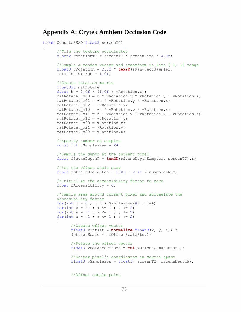
75
Appendix A: Crytek Ambient Occlusion Code
float ComputeSSAO(float2 screenTC)
{
//Tile the texture coordinates
float2 rotationTC = screenTC * screenSize / 4.0f;
//Sample a random vector and transform it into [-1, 1] range
float3 vRotation = 2.0f * tex2D(sRandVectSampler,
rotationTC).rgb - 1.0f;
//Create rotation matrix
float3x3 matRotate;
float h = 1.0f / (1.0f + vRotation.z);
matRotate._m00 = h * vRotation.y * vRotation.y + vRotation.z;
matRotate._m01 = -h * vRotation.y * vRotation.x;
matRotate._m02 = -vRotation.x;
matRotate._m10 = -h * vRotation.y * vRotation.x;
matRotate._m11 = h * vRotation.x * vRotation.x + vRotation.z;
matRotate._m12 = -vRotation.y;
matRotate._m20 = vRotation.x;
matRotate._m21 = vRotation.y;
matRotate._m22 = vRotation.z;
//Specify number of samples
const int nSamplesNum = 24;
//Sample the depth at the current pixel
float fSceneDepthP = tex2D(sSceneDepthSampler, screenTC).r;
//Set the offset scale step
float fOffsetScaleStep = 1.0f + 2.4f / nSamplesNum;
//Initialize the accessibility factor to zero
float fAccessibility = 0;
//Sample area around current pixel and accumulate the
accessibility factor
for(int i = 0 ; i < (nSamplesNum/8) ; i++)
for(int x = -1 ; x <= 1 ; x += 2)
for(int y = -1 ; y <= 1 ; y += 2)
for(int z = -1 ; z <= 1 ; z += 2)
{
//Create offset vector
float3 vOffset = normalize(float3(x, y, z)) *
(offsetScale *= fOffsetScaleStep);
//Rotate the offset vector
float3 vRotatedOffset = mul(vOffset, matRotate);
//Center pixel's coordinates in screen space
float3 vSamplePos = float3( screenTC, fSceneDepthP);
//Offset sample point
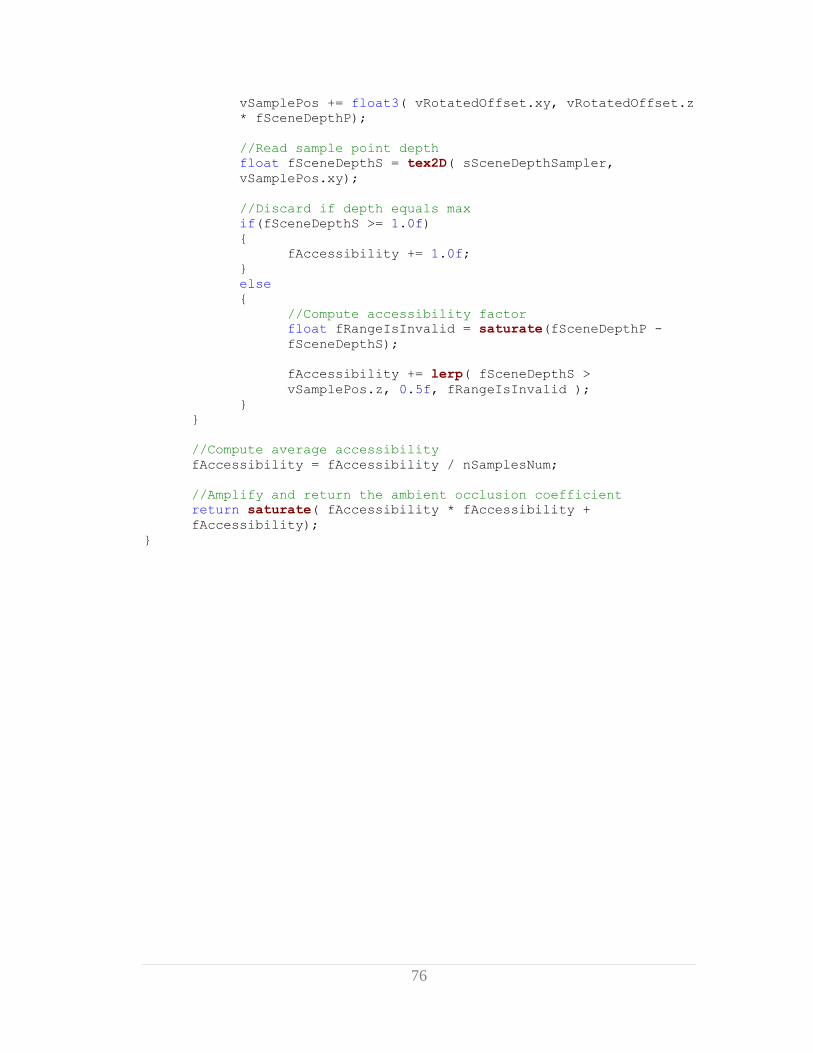
76
vSamplePos += float3( vRotatedOffset.xy, vRotatedOffset.z
* fSceneDepthP);
//Read sample point depth
float fSceneDepthS = tex2D( sSceneDepthSampler,
vSamplePos.xy);
//Discard if depth equals max
if(fSceneDepthS >= 1.0f)
{
fAccessibility += 1.0f;
}
else
{
//Compute accessibility factor
float fRangeIsInvalid = saturate(fSceneDepthP -
fSceneDepthS);
fAccessibility += lerp( fSceneDepthS >
vSamplePos.z, 0.5f, fRangeIsInvalid );
}
}
//Compute average accessibility
fAccessibility = fAccessibility / nSamplesNum;
//Amplify and return the ambient occlusion coefficient
return saturate( fAccessibility * fAccessibility +
fAccessibility);
}
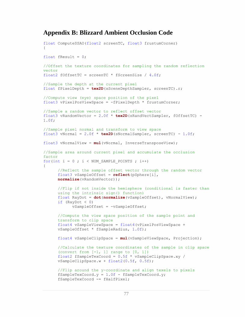
77
Appendix B: Blizzard Ambient Occlusion Code
float ComputeSSAO(float2 screenTC, float3 frustumCorner)
{
float fResult = 0;
//Offset the texture coordinates for sampling the random reflection
vector
float2 fOffsetTC = screenTC * fScreenSize / 4.0f;
//Sample the depth at the current pixel
float fPixelDepth = tex2D(sSceneDepthSampler, screenTC).r;
//Compute view (eye) space position of the pixel
float3 vPixelPosViewSpace = -fPixelDepth * frustumCorner;
//Sample a random vector to reflect offset vector
float3 vRandomVector = 2.0f * tex2D(sRandVectSampler, fOffsetTC) -
1.0f;
//Sample pixel normal and transform to view space
float3 vNormal = 2.0f * tex2D(sNormalSampler, screenTC) - 1.0f;
float3 vNormalView = mul(vNormal, InverseTransposeView);
//Sample area around current pixel and accumulate the occlusion
factor
for(int i = 0 ; i < NUM_SAMPLE_POINTS ; i++)
{
//Reflect the sample offset vector through the random vector
float3 vSampleOffset = reflect(pSphere[i],
normalize(vRandomVector));
//Flip if not inside the hemisphere (conditional is faster than
using the intrinsic sign() function)
float RayDot = dot(normalize(vSampleOffset), vNormalView);
if (RayDot < 0)
vSampleOffset = -vSampleOffset;
//Compute the view space position of the sample point and
transform to clip space
float4 vSampleViewSpace = float4(vPixelPosViewSpace +
vSampleOffset * fSampleRadius, 1.0f);
float4 vSampleClipSpace = mul(vSampleViewSpace, Projection);
//Calculate the texture coordinates of the sample in clip space
(convert from [-1, 1] range to [0, 1])
float2 fSampleTexCoord = 0.5f * vSampleClipSpace.xy /
vSampleClipSpace.w + float2(0.5f, 0.5f);
//Flip around the y-coordinate and align texels to pixels
fSampleTexCoord.y = 1.0f - fSampleTexCoord.y;
fSampleTexCoord -= fHalfPixel;
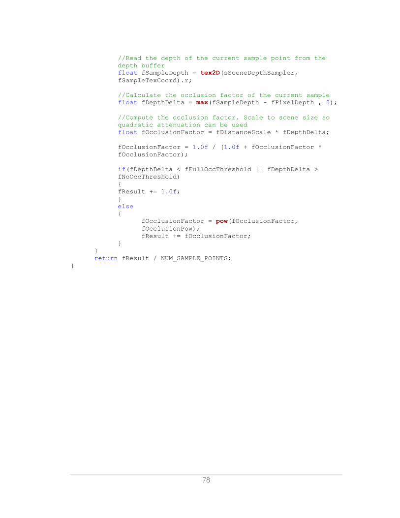
78
//Read the depth of the current sample point from the
depth buffer
float fSampleDepth = tex2D(sSceneDepthSampler,
fSampleTexCoord).r;
//Calculate the occlusion factor of the current sample
float fDepthDelta = max(fSampleDepth - fPixelDepth , 0);
//Compute the occlusion factor. Scale to scene size so
quadratic attenuation can be used
float fOcclusionFactor = fDistanceScale * fDepthDelta;
fOcclusionFactor = 1.0f / (1.0f + fOcclusionFactor *
fOcclusionFactor);
if(fDepthDelta < fFullOccThreshold || fDepthDelta >
fNoOccThreshold)
{
fResult += 1.0f;
}
else
{
fOcclusionFactor = pow(fOcclusionFactor,
fOcclusionPow);
fResult += fOcclusionFactor;
}
}
return fResult / NUM_SAMPLE_POINTS;
}
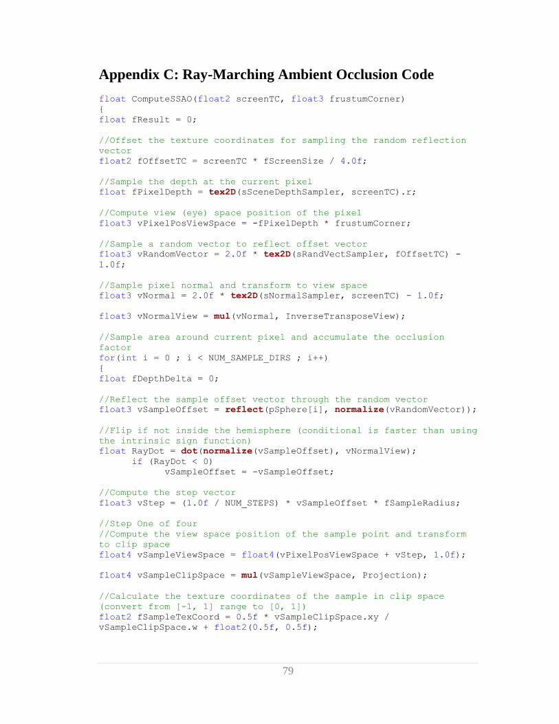
79
Appendix C: Ray-Marching Ambient Occlusion Code
float ComputeSSAO(float2 screenTC, float3 frustumCorner)
{
float fResult = 0;
//Offset the texture coordinates for sampling the random reflection
vector
float2 fOffsetTC = screenTC * fScreenSize / 4.0f;
//Sample the depth at the current pixel
float fPixelDepth = tex2D(sSceneDepthSampler, screenTC).r;
//Compute view (eye) space position of the pixel
float3 vPixelPosViewSpace = -fPixelDepth * frustumCorner;
//Sample a random vector to reflect offset vector
float3 vRandomVector = 2.0f * tex2D(sRandVectSampler, fOffsetTC) -
1.0f;
//Sample pixel normal and transform to view space
float3 vNormal = 2.0f * tex2D(sNormalSampler, screenTC) - 1.0f;
float3 vNormalView = mul(vNormal, InverseTransposeView);
//Sample area around current pixel and accumulate the occlusion
factor
for(int i = 0 ; i < NUM_SAMPLE_DIRS ; i++)
{
float fDepthDelta = 0;
//Reflect the sample offset vector through the random vector
float3 vSampleOffset = reflect(pSphere[i], normalize(vRandomVector));
//Flip if not inside the hemisphere (conditional is faster than using
the intrinsic sign function)
float RayDot = dot(normalize(vSampleOffset), vNormalView);
if (RayDot < 0)
vSampleOffset = -vSampleOffset;
//Compute the step vector
float3 vStep = (1.0f / NUM_STEPS) * vSampleOffset * fSampleRadius;
//Step One of four
//Compute the view space position of the sample point and transform
to clip space
float4 vSampleViewSpace = float4(vPixelPosViewSpace + vStep, 1.0f);
float4 vSampleClipSpace = mul(vSampleViewSpace, Projection);
//Calculate the texture coordinates of the sample in clip space
(convert from [-1, 1] range to [0, 1])
float2 fSampleTexCoord = 0.5f * vSampleClipSpace.xy /
vSampleClipSpace.w + float2(0.5f, 0.5f);

80
//Flip around the y-coordinate and align texels to pixels
fSampleTexCoord.y = 1.0f - fSampleTexCoord.y;
fSampleTexCoord -= fHalfPixel;
//Read the depth of the current sample point from the depth buffer
float fSampleDepth = tex2D(sSceneDepthSampler, fSampleTexCoord).r;
fDepthDelta = max(fSampleDepth - fPixelDepth , 0);
//Step Two of four
if(fDepthDelta < fFullOccThreshold)
{
//Compute the view space position of the sample point and transform
to clip space
vSampleViewSpace = float4(vSampleViewSpace + vStep, 1.0f);
vSampleClipSpace = mul(vSampleViewSpace, Projection);
//Calculate the texture coordinates of the sample in clip space
(convert from [-1, 1] range to [0, 1])
fSampleTexCoord = 0.5f * vSampleClipSpace.xy / vSampleClipSpace.w +
float2(0.5f, 0.5f);
//Flip around the y-coordinate and align texels to pixels
fSampleTexCoord.y = 1.0f - fSampleTexCoord.y;
fSampleTexCoord -= fHalfPixel;
//Read the depth of the current sample point from the depth buffer
fSampleDepth = tex2D(sSceneDepthSampler, fSampleTexCoord).r;
fDepthDelta = max(fSampleDepth - fPixelDepth , 0);
}
//Step Three of four
if(fDepthDelta < fFullOccThreshold)
{
//Compute the view space position of the sample point and transform
to clip space
vSampleViewSpace = float4(vSampleViewSpace + vStep, 1.0f);
vSampleClipSpace = mul(vSampleViewSpace, Projection);
//Calculate the texture coordinates of the sample in clip space
(convert from [-1, 1] range to [0, 1])
fSampleTexCoord = 0.5f * vSampleClipSpace.xy / vSampleClipSpace.w +
float2(0.5f, 0.5f);
//Flip around the y-coordinate and align texels to pixels
fSampleTexCoord.y = 1.0f - fSampleTexCoord.y;
fSampleTexCoord -= fHalfPixel;
//Read the depth of the current sample point from the depth buffer
fSampleDepth = tex2D(sSceneDepthSampler, fSampleTexCoord).r;
fDepthDelta = max(fSampleDepth - fPixelDepth , 0);
}
//Step Four of four
81
if(fDepthDelta < fFullOccThreshold)
{
//Compute the view space position of the sample point and transform
to clip space
vSampleViewSpace = float4(vSampleViewSpace + vStep, 1.0f);
vSampleClipSpace = mul(vSampleViewSpace, Projection);
//Calculate the texture coordinates of the sample in clip space
(convert from [-1, 1] range to [0, 1])
fSampleTexCoord = 0.5f * vSampleClipSpace.xy / vSampleClipSpace.w +
float2(0.5f, 0.5f);
//Flip around the y-coordinate and align texels to pixels
fSampleTexCoord.y = 1.0f - fSampleTexCoord.y;
fSampleTexCoord -= fHalfPixel;
//Read the depth of the current sample point from the depth buffer
fSampleDepth = tex2D(sSceneDepthSampler, fSampleTexCoord).r;
fDepthDelta = max(fSampleDepth - fPixelDepth , 0);
}
//Calculate the occlusion factor of the current sample
float occlusionFactor = (fDistanceScale * fDepthDelta);
occlusionFactor = 1.0f / (1.0f + occlusionFactor * occlusionFactor);
if(fDepthDelta < fFullOccThreshold || fDepthDelta > fNoOccThreshold)
fResult += 1.0f;
else
{
occlusionFactor = pow(occlusionFactor, fOcclusionPow);
fResult += occlusionFactor;
}
}
return fResult / NUM_SAMPLE_DIRS;
}

82
Appendix D: Experiment Instructions
In this experiment you will be asked to evaluate the visual realism of a series of
rendered images. A total of 14 images will be displayed in pairs of two. Your task is
to determine which image in each pair you think looks the most realistic. For each
image pair the procedure is the following:
The first image will be displayed and you are free to examine it for as long as you
wish. When done examining the first image, press the spacebar to queue the next
image. After pressing the spacebar, a grey image will be displayed for two seconds
which you cannot skip. After the grey image, the second image will be displayed.
Again, you will have as long as you decide is necessary to examine the image. When
done with the second image, press the spacebar again to end the current comparison
task. After each comparison task, a message box will be displayed requiring you to
select which image you found the most realistic.
Please note that direct comparison between images is not possible, and once you are
done examining an image, you will not have the opportunity to view it again. Also,
there is no right or wrong answer and if you are in doubt, go with your intuition or
initial impression. If you have any questions please ask, otherwise press the button
below to begin the experiment.

83
Appendix E: Stimuli Pair I – Dragon Low
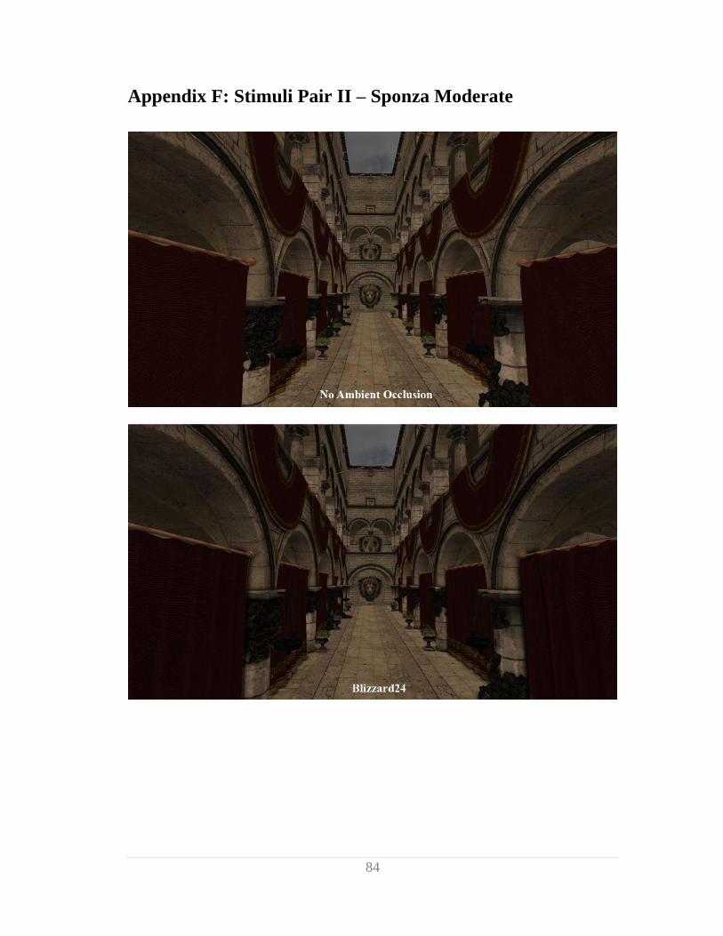
84
Appendix F: Stimuli Pair II – Sponza Moderate
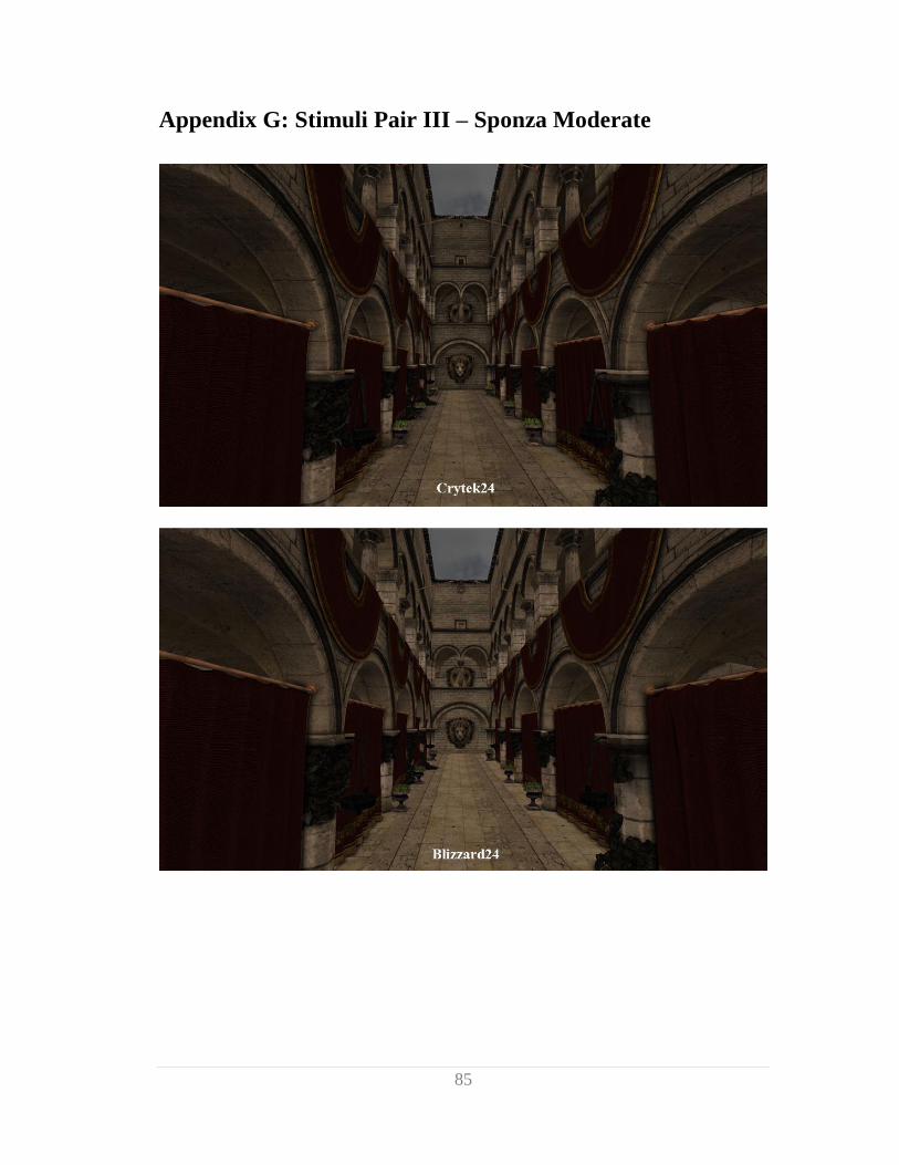
85
Appendix G: Stimuli Pair III – Sponza Moderate
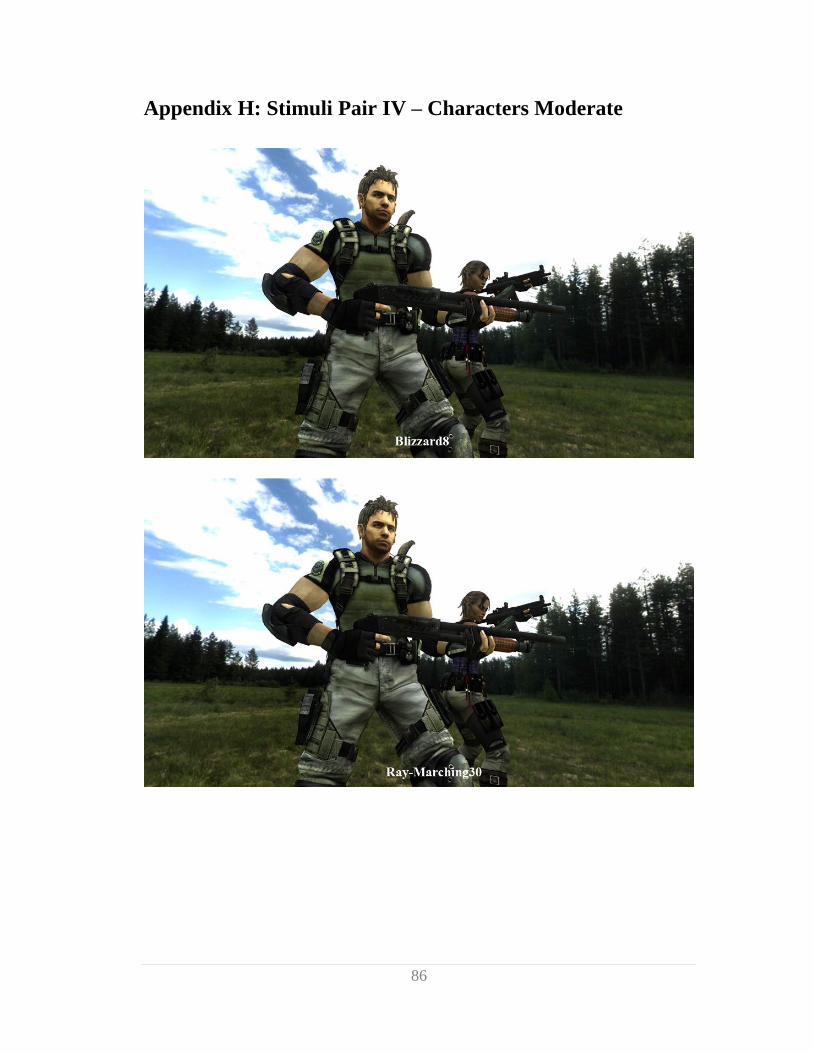
86
Appendix H: Stimuli Pair IV – Characters Moderate
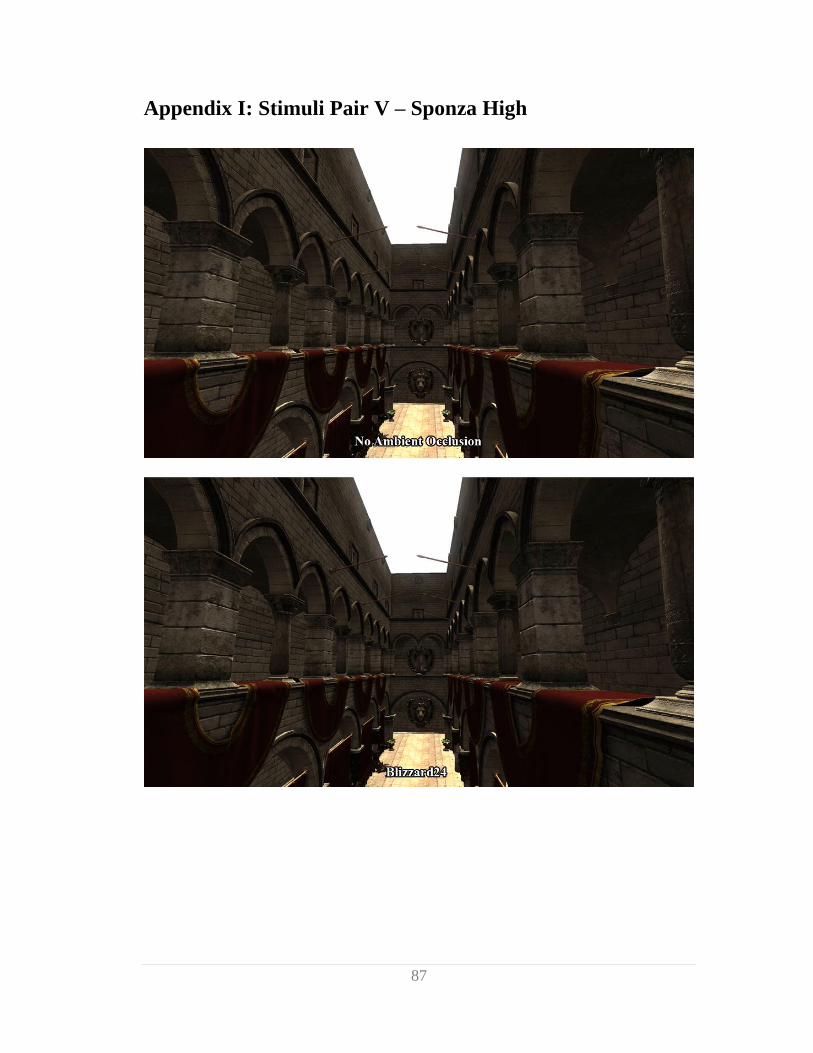
87
Appendix I: Stimuli Pair V – Sponza High
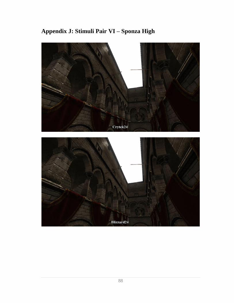
88
Appendix J: Stimuli Pair VI – Sponza High
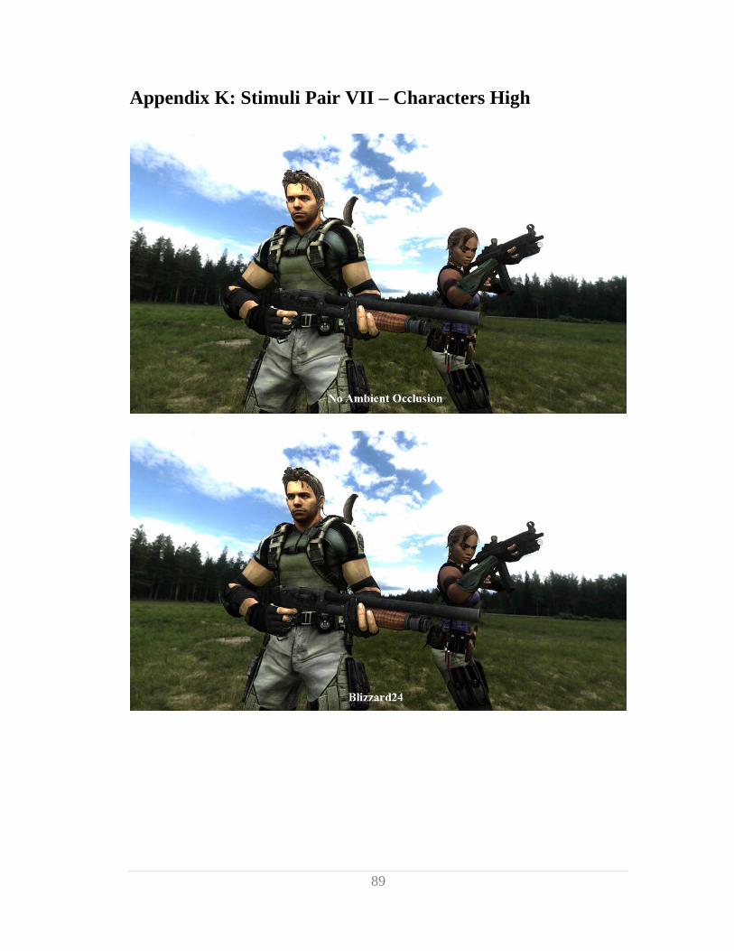
89
Appendix K: Stimuli Pair VII – Characters High
90
Glossary
Acceleration Structure: A programmatic construct used to partition the geometry of
a scene into sections. Intersection tests with rays can then be performed on these top-
level sections to determine if the ray intersects geometry contained within the section.
If no intersection is found, all the geometry inside the section is skipped, speeding up
intersection testing greatly.
Bidirectional reflectance distribution function: A function describing how light is
reflected from a surface. Two directions are used in the function, the incoming light
direction and the outgoing view direction.
Depth Buffer: A buffer holding the depth of all visible pixels.
Gold Standard: A reference image used to compare approximations with in
psychophysical experiments. It is usually a real-world image or a physically accurate
synthetic rendering.
Ground Truth: See Gold standard.
Irradiance: A measure of light incoming to a point from all directions in the
hemisphere
Irradiance Environment Mapping: The process of using a heavily blurred
environment map representing the scene to calculate irradiance. The process results in
more shading variation in the indirect lighting than using a constant ambient light.
Jittering: Commonly defined as small rapid variations in a waveform. In the context
of graphics programming, it is often used to indicate the process of creating a high-
frequency random distribution of samples.
Lambertian Diffuse: A perfectly diffuse surface where light is scattered evenly in all
directions.
91
Normal Mapping: A subset of bump mapping where modified normals are stored in
a texture map which are then used in lighting calculations instead of the actual surface
normals. This process results in shading that mimics geometry which is not actually
there, creating additional surface detail.
Object-Space: 3D coordinate space. Object-space is defined locally for each object
meaning that the origin is defined in some relation to a point on the object, e.g. the
pelvis of a character model.
Radiance: A measure of light in a single ray
Screen-Space: The coordinate space after the 3D scene has been projected to 2D. The
X and Y coordinates can be used with the Z-value from the depth buffer to
reconstruct world- or view-space 3D positions.
Spherical Proxy: An approximate reconstruction of the surface underlying the
sample pixel using a sphere. Can either be actual geometry or a mathematical
construct used in an equation.
Surface Normal: A vector standing perpendicular to a surface, usually just referred
to as the normal.
View-Space: Coordinate space relative to the virtual camera. The world-space
coordinates are transformed so that the camera is placed at the origin and is looking
down the z-axis into the scene.
World-Space: 3D coordinate space that defines where objects are placed and
oriented in relation to each other.

92
This page is intentionally left blank.
93
Bibliography
Bartz, Dirk, Douglas Cunningham, Jan Fischer, and Christian Wallraven. “The Role
of Perception for Computer Graphics.” Proceedings of the 29th Annual
Conference Eurographics. Oxford, United Kingdom: The Eurographics
Association, 2008. 65-86.
Bavoil, Louis, and Miguel Sainz. “Image-Space Horizon-Based Ambient Occlusion.”
In ShaderX7, by Wolfgang Engel, 425-444. Boston, MA: Course Technology,
2009.
Cook, Robert L., and Kenneth E. Torrance. “A Reflectance Model for Computer
Graphics.” International Conference on Computer Graphics and Interactive
Techniques. Dallas, Texas: ACM, 1981. 307-316.
Crytek. Crysis. Frankfurt, November 2007.
Daly, Scott. “The Visible Differences Predictor: An Algorithm for the Assessment of
Image Fidelity.” In Digital Images and Human Vision, by Andrew B. Watson,
179-206. Cambridge, Massachusets: MIT Press, 1993.
Filion, Dominic, and Rob McNaughton. "StarCraft II - Effects & techniques."
International Conference on Computer Graphics and Interactive Techniques.
Los Angeles: ACM, 2008. 133-164.
Goral, Cindy M, Kenneth E Torrance, Donald P Greenberg, and Bennet Battaile.
“Modeling the Interaction of Light Between Diffuse Surfaces.” International
Conference on Computer Graphics and Interactive Techniques. New York:
ACM, 1984. 213-222.
Jensen, Henrik Wann. “Global Illumination Using Photon Maps.” Proceedings of the
eurographics workshop on Rendering techniques '96. London: Springer-
Verlag, 1996. 21-30.
94
Jimenez, Jorge, Veronica Sundstedt, and Diego Gutierrez. "Screen-Space Perceptual
Rendering of Human Skin." Applied Perception in Graphics and
Visualization. Chania, Greece: ACM, 2009.
Kajalin, Vladimir. “Screen-Space Ambient Occlusion.” In ShaderX7, by Wolfgang
Engel, 413-424. Boston, MA: Course Technology, 2009.
Kozlowski, Oscar, and Jan Kautz. "Is Accurate Occlusion of Glossy Reflections
Necessary." Applied Perception in Graphics and Visualization. Tubingen,
Germany: ACM, 2007. 91-98.
McNamara, Ann. “Exploring Visual and Automatic Measures of Perceptual Fidelity
in Real and Simulated Imagery.” ACM Transactions on Applied Perception
(ACM) 3, no. 3 (July 2006): 217-238.
McNamara, Ann. “Visual Perception in Realistic Image Synthesis.” Computer
Graphics Forum 20, no. 4 (2001): 211-224.
Mittring, Martin. “Finding next gen: CryEngine 2.” International Conference on
Computer Graphics and Interactive Techniques. San Diego: ACM, 2007. 97-
121.
Möller, Tomas Akenine, Eric Haines, and Naty Hoffman. Real-Time Rendering.
Wellesley, Massachusetts: A K Peters, Ltd., 2008.
Palmer, Stephen E. Vision Science - Photons to Phenomenology. Cambridge,
Massachusetts: The MIT Press, 1999.
Ritschel, Tobias, Thorsten Grosch, and Hans-Peter Seidel. "Approximating Dynamic
Global Illumination in Image Space." Symposium on Interactive 3D Graphics.
Boston: ACM, 2009. 75-82.
95
Robertson, Barbara. “CG Society.” Shades of Davy Jones. 22 December 2006.
http://features.cgsociety.org/story_custom.php?story_id=3889 (accessed May
15, 2010).
Shanmugam, Perumaal, and Okan Arikan. "Hardware Accelerated Ambient
Occlusion Techniques on GPUs." Symposium on Interactive 3D Graphics.
Seattle: ACM, 2007. 73-80.
Sundstedt, Veronica, Diego Gutierrez, Oscar Anson, Franscesco Banterle, and Alan
Chalmers. "Perceptual Rendering of Participating Media." ACM Transactions
on Applied Perception. ACM, 2007.
Wang, Rui, Kun Zhou, Minghao Pan, and Hujun Bao. “An Efficient GPU-Based
Approach for Interactive Global Illumination.” International Conference on
Computer Graphics and Interactive Techniques. New Orleans, Louisiana:
ACM, 2009.
Yu, Insu, et al. "Perceptual Influence of Approximate Visibility in Indirect
Illumination." Applied Perception in Graphics and Visualization. Chania:
ACM, 2009.
Zhukov, Sergei, and Andrei Iones. “An Ambient Light Illumination Model.” 9th
Eurographics Workshop on Rendering, 1998: 45-56.
Recommended