The Micro Economics of Efficient Group
Behavior: Identification∗
P.A. Chiappori† I. Ekeland‡
Revised version
November 2006
Abstract
Consider a group consisting of S members facing a common budget
constraint p0ξ = 1; any demand vector belonging to the budget set can
be (privately or publicly) consumed by the members. Although the
∗ Paper presented at seminars in Chicago, Paris, Tel Aviv, New York, Banff andLondon. We thank the participants for their suggestions. This research received financialsupp ort f rom the NSF ( grant SBR 0532398).
† Corresp onding authorDepartment of Economics, Columbia University. Email: [email protected]
‡Canada Research Chair in Mathematical Economics, the University of BritishColumbia. Adress: PIMS, 1933 West Mall, UBC, Vancouver BC, V6T 1Z2 Canada. E-mail: [email protected]
1

intra-group decision process is not known, it is assumed to generate
Pareto efficient outcomes; neither individual consumptions nor intra-
group transfers are observable. The paper analyzes when, to what
extent and under which conditions it is possible to recover the under-
lying structure - individual preferences and the decision process - from
the group’s aggregate behavior. We show that the general version of
the model is not identified. However, a simple exclusivity assumption
(whereby each member is the exclusive consumer of at least one good)
is sufficient to guarantee generic identifiability of the welfare-relevant
structural concepts.
2

1 Introduction
Group behavior: beyond the ’black box’ Consider a group consisting
of S members. The group has limited resources; specifically, its global con-
sumption vector ξ must satisfy a standard market budget constraint of the
form p0ξ = y (where p is a vector of prices and y is total group income). Any
demand vector belonging to the global budget set thus defined can be con-
sumed by the members. Some of the goods can be privately consumed, while
others may be publicly used. The decision process within the group is not
known, and is only assumed to generate Pareto efficient outcomes1. Finally,
neither individual consumptions nor intragroup transfers are observable. In
other words, the group is perceived as a ’black box’; only its aggregate be-
havior, summarized by the demand function ξ (p, y), is recorded. The goal
of the present paper is to provide answers to the general question: when is it
1We view efficiency as a natural assumption in many contexts, and as a natural bench-mark in all cases. For instance, the analysis of household behavior often takes the ’col-lective’ point of view, where efficiency is the basic postulate. Other models, in particularin the literature on firm behavior, are based on cooperative game theory in a symmetricinformation context, where efficiency is paramount (see for instance the ’insider-outsider’literature, and more generally the models involving bargaining between management andworkers or unions). The analysis of intra group risk sharing, starting with Townsend’sseminal paper (1994), provides other interesting examples. Finally, even in the presence ofasymmetric information, first best efficiency is a natural benchmark. For instance, a largepart of the empirical literature on contract theory tests models involving asymmetric infor-mation against the null of symmetric information and first best efficiency (see Chiapporiand Salanie (2000) for a recent survey).
3
possible to recover the underlying structure - namely, individual preferences,
the decision process and the resulting intragroup transfers - from the group’s
aggregate behavior?
In the (very) particular case where the group consists of only one member,
the answer is well known: individual demand uniquely defines the underly-
ing preferences. Not much is known in the case of a larger group. However,
recent results in the literature on household behavior suggest that, surpris-
ingly enough, when the group is ’small’, the structure can be recovered under
reasonably mild assumptions. For instance, in the model of household labor
supply proposed by Chiappori (1988, 1992), two individuals privately con-
sume leisure and some Hicksian composite good. The main conclusion is
that the two individual preferences and the decision process can generically
be recovered (up to an additive constant) from the two labor supply func-
tions. This result has been empirically applied (among others) by Fortin
and Lacroix (1997) and Chiappori, Fortin and Lacroix (2002), and extended
by Chiappori (1997) to household production and by Blundell et al. (2000)
to discrete participation decisions. Fong and Zhang (2001) consider a more
general model where leisure can be consumed both privately and publicly.
Although the two alternative uses are not independently observed, they can
4

in general be identified under a separability restriction, provided that the
consumption of another exclusive good (e.g. clothing) is observed.
Altogether, these results suggest that there is information to be gained
on the contents of the ’black box’. In a companion paper (Chiappori and
Ekeland 2006), we investigate the properties of aggregate behavior stemming
from the efficiency assumption. We conclude that when the group is small
enough, a lot of structure is imposed on collective demand by this basic
assumption: there exist strong, testable, restrictions on the way the black
box may operate. The main point of the present paper is complementary.
We investigate to what extent, and under which conditions, it is possible
to recover much (or all) of the interior structure of the black box without
opening it. We first show that in the most general case, there exists a con-
tinuum of observationally equivalent models - i.e. a continuum of different
structural settings generating identical observable behavior. This negative
result implies that additional assumptions are required.
We then provide examples of such assumptions, and show that they are
surprisingly mild. Essentially, it is sufficient that each agent in the group
be the exclusive consumer of (at least) one commodity. Moreover, when a
‘distribution factor’ (see below) is available, this requirement can be reduced
5

to the existence of an assignable good (i.e., a private good for which individual
consumptions are observed). Under these conditions, the structure that is
relevant to formulate welfare judgments is non parametrically identified in
general (in a sense that is made clear below), irrespective of the total number
of commodities. We conclude that even when decision processes or intra
group transfers are not known, much can be learned about them from the sole
observation of the group’s aggregate behavior. This conclusion generalizes
the earlier intuition of Chiappori (1988, 1992); it shows that the results
obtained in these early contributions, far from being specific to the particular
settings under consideration, were in fact general.
Identifiability and identification From a methodological perspective, it
may be useful to define more precisely what is meant by ’recovering the un-
derlying structure’. The structure, in our case, is defined by the (strictly
convex) preferences of individuals in the group and the decision process.
Because of the efficiency assumption, for any particular cardinalization of
individual utilities the decision process is fully summarized by the Pareto
weights corresponding to the outcome at stake. The structure, thus, con-
sists in a set of individual preferences (with a particular cardinalization) and
6

Pareto weights (with some normalization - e.g., the sum of Pareto weights is
taken to be one).
This structure is not observable; what can be recorded is the group’s
aggregate demand function ξ (p, y). In practice, the ’observation’ of ξ (p, y)
is a complex process, that entails specific difficulties. For instance, one never
observes a (continuous) function, but only a finite number of values on the
function’s graph. These values are measured with some errors, which raises
problems of statistical inference. In some cases, the data are cross-sectional,
in the sense that different groups are observed in different situations; specific
assumptions have to be made on the nature and the form of (observed and
unobserved) heterogeneity between the groups. Even when the same group
is observed in different contexts (say, from panel data), other assumptions
are needed on the dynamics of the situation, e.g. on the way past behavior
influences present choices. All these issues, which lay at the core of what is
usually called the identification problem, are outside the scope of the paper.
Our interest, here, is in what has been called the identifiability problem,
which can be defined as follows: when is it the case that the (hypothetically)
perfect knowledge of a smooth demand function ξ (p, y) uniquely defines the
underlying structure within a given class? Formally, for any given structure,
7
the maximization of the (Pareto) weighted sum of utilities generates a unique
demand function. This defines a mapping from the set of structures to the
set of demand functions. Identifiability obtains if this mapping is injective,
in the sense that two different structures can never generate the same de-
mand function. In other words, non identifiability does not result from the
econometrician’s inability to exactly recover the form of demand functions
- say, because only noisy estimates of the parameters can be obtained, or
even because the functional form itself (and the stochastic structure added
to it) have been arbitrarily chosen. These econometric questions have, at
least to some extent, econometric or statistical answers. For instance, confi-
dence intervals can be computed for the parameters (and become negligible
when the sample size grows); the relevance of the functional form can be
checked using specification tests; etc. The non identifiability problem has a
different nature: even if a perfect fit to ideal data was feasible, it would still
be impossible to recover the underlying structure from observed behavior.2
In the case of individual behavior, as analyzed by standard consumer the-
2The distinction between identification and identifiability can be traced back to Koop-mans’s (1949) seminal paper (we thank Martin Browning for suggesting this reference).A difference is that Koopmans’s defines a ’structure’ as ’a combination of a specific setof structural equations and a specific distribution function of the latent variables’ - a’model’ being defined as a ’set of structures’. Koopmans clearly distinguishes two typesof identification problems, namely those linked with ’statistical inference’ and those dueto ’identifiablity’.
8

ory, identifiability is an old but crucial result. Indeed, it has been known for
more than a century that an individual demand function uniquely identifies
the underlying preferences. Usual as this property may have become, it re-
mains one of the strongest results in microeconomic theory. It implies, for
instance, that assessments about individual well-being can unambiguously
be made from the sole observation of demand behavior - a fact that opens
the way to all of applied welfare economics. The present work can be seen as
an attempt at generalizing this classical identifiability property to efficient
groups of arbitrary sizes.
Identifiability is a necessary condition for identification. If different struc-
tures are observationally equivalent, there is no hope that observed behavior
will help to distinguish between them - only ad hoc functional form restric-
tions can do that. Since observationally equivalent models may have very
different welfare implications, non identifiability severely limits our ability
to formulate reliable normative judgments: any normative recommendation
based on a particular structural model is unreliable, since it is ultimately
based on the purely arbitrary choice of one underlying structural model
among many.
Note, finally, that identifiability is only a necessary first step for identifi-
9

cation (in the standard, econometric sense). Whether an identifiable model is
econometrically identified depends on the stochastic structure representing
the various statistical issues (measurement errors, unobserved heterogene-
ity,...) discussed above. After all, the abundant empirical literature on con-
sumer behavior, while dealing with a model that is always identifiable, has
convinced us that identification crucially depends on the nature of available
data.
Parametric versus non-parametric identifiability The identifiability
problem may be approached from a parametric or a non parametric perspec-
tive. In the parametric approach, a particular functional form is chosen for
the structural model, and a reduced form for the demand function is derived.
In particular, the derivation highlights the links between the parameters of
the structural model and the coefficient of the demand function that will be
taken to data. Identification, in this context, is equivalent to the uniqueness
of the set of parameters of the structural model corresponding to any speci-
fied values for the (estimated) coefficients of the reduced form. Note that in
such a context, uniqueness or identifiability are conditional on the functional
form; i.e. it obtains (at best) within a specific and narrow set of candidate
10

functions, namely those compatible with the functional form chosen at the
outset.
Throughout this paper, our approach, on the contrary, is explicitly non-
parametric. That is, we try to find conditions that guarantee uniqueness
within the general class of smooth, strictly convex preferences and differen-
tiable Pareto weights. One can readily provide examples in which identifi-
ability obtains in a parametric sense, but not in the non-parametric setting
(it is then functional form dependent)3.
In practice, parametric models are often convenient. In particular, we do
not suggest that parametric estimations should not be used, or even that it
should be resorted to with some reluctance. Postulating a specific functional
form is a standard, well established and often extremely fruitful methodol-
ogy. We do however submit that the status of the conclusions drawn from
parametric estimations crucially depend on whether or not the underlying
model is non-parametrically identifiable. If it is, then the reliability of the
parametric estimates (and, consequently, of the conclusions drawn from it)
is directly related to the quality of the empirical fit, as assessed by standard
econometric tests. If the econometrician can convince himself (and the scien-
3See for instance Blundell, Chiappori and Meghir (2006).
11

tific community) that the model provides a pretty faithful representation of
the real phenomenon, then the same level of trust could in principle be put
into the conclusions derived from it. The case is much weaker in the absence
of non parametric identifiability. A good empirical fit is no longer sufficient:
by definition, many different structural models, with potentially divergent
normative implications, have exactly the same fit (since they generate the
same reduced forms), hence are exactly as well supported by the data as the
initial one.
Of course, this discussion should not be interpreted too strictly. In the
end, identifying assumptions are (almost) always needed. The absence of
non parametrically identifiability, thus, should not necessarily be viewed as
a major weakness. We believe, however, that it justifies a more cautious
interpretation of the estimates. More importantly, we submit, as a basic,
methodological rule, that an explicit analysis of non parametric identifiabil-
ity is a necessary first step in any consistent empirical strategy - if only to
suggest the most adequate identifying assumptions. Applying this approach
to collective models is indeed the main purpose of this paper.
12

Distribution factors An important tool to achieve identification is the
presence of distribution factors; see Bourguignon, Browning and Chiappori
(1995). These are defined as variables that can affect group behavior only
through their impact on the decision process. Think, for instance, of the
choices as resulting from a bargaining process. Typically, the outcomes will
depend on the members’ respective bargaining positions; hence, any factor of
the group’s environment that may influence these positions (EEPs in McEl-
roy’s (1990) terminology) potentially affects the outcome. Such effects are of
course paramount, and their relevance is not restricted to bargaining in any
particular sense. In general, group behavior depends not only on preferences
and budget constraint, but also on the members’ respective ’power’ in the
decision process. Any variable that changes the powers may have an impact
on observed collective behavior.
In many cases, distribution factors are readily observable. An example is
provided by the literature on household behavior. In their study of house-
hold labor supply, Chiappori, Fortin and Lacroix (2002) use the state of the
marriage market, as proxied by the sex ratio by age, race and state, and
the legislation on divorce, as particular distribution factors affecting the in-
trahousehold decision process, and thereby its outcome, i.e. labor supplies.
13

They find, indeed, that factors more favorable to women significantly de-
crease (resp. increase) female (resp. male) labor supply. Using similar tools,
Oreffice (2005) concludes that the legalization of abortion had a significant
impact on intrahousehold allocation of power. In a similar context, Rubal-
cava and Thomas (2000) use the generosity of single parent benefits and
reach identical conclusions. Thomas, Contreras, and Frankenberg(1997), us-
ing an Indonesian survey, show that the distribution of wealth by gender at
marriage - another candidate distribution factor - has a significant impact on
children health in those areas where wealth remains under the contributor’s
control4. Duflo (2000) has derived related conclusions from a careful analy-
sis of a reform of the South African social pension program that extended
the benefits to a large, previously not covered black population. She finds
that the recipient’s gender - a typical distribution factor - is of considerable
importance for the consequences of the transfers on children’s health.
Whenever the aggregate group demand is observable as a function of
prices and distribution factors, one can expect that identification may be
easier to obtain. This is actually known to be the case in particular situ-
ations. For instance, Chiappori, Fortin and Lacroix (2002) show how the
4See also Galasso (1999) for a similar investigation.
14

use of distribution factors allows a simpler and more robust estimation of a
collective model of labor supply. In the present paper, we generalize these
results by providing a general analysis of the estimation of collective models
in different contexts, with and without distribution factors.
The results Our main conclusions can be summarized as follows:
• In its most general formulation, the model is not identifiable. Any given
aggregate demand that is compatible with efficiency can be derived
either from a model with private consumption only, or from a model
with public consumption only. Moreover, even when it is assumed
that all consumptions are private (or that they are all public, or that
some commodities are privately and other publicly consumed), in the
absence of exclusive consumptions there exists a continuum of different
structural models that generate the same aggregate demand. More
precisely, identifiability obtains only up to two functions, in a manner
that is precisely described in the paper.
• A simple exclusivity assumption is in general sufficient to guarantee full,
non-parametric identifiability of the welfare-relevant structure. Specif-
ically, we define the collective indirect utility of each member as the
15

utility level that member ultimately reaches for given prices, house-
hold income and possibly distribution factors, taking into account the
allocation of resources prevailing within the household. We show the
following result: if, for each agent of the group, there exists a commod-
ity which is exclusively consumed by that agent, then, in general, the
collective indirect utility of each member can be recovered (up to some
increasing transform), irrespective of the total number of commodi-
ties. Our general conclusion, hence, is that one exclusive commodity
per agent is sufficient to identify all welfare-relevant aspects of the col-
lective model. Moreover, when distribution factors are available, one
assignable good (i.e., a private good for which individual consumptions
are observed) only is sufficient for identifiability.
Section 2 describes the model. The formal structure of the identifiability
problem is analyzed in Section 3. Sections 4, 5 and 6 consider the case of
two-person groups. Section 4 characterizes the limits to identification in a
general context. Identification under exclusivity or generalized separability
assumptions is discussed in Section 5, and applied to specific economic frame-
works in Section 6. Section 7 briefly discusses the extension to the general
case of S-person groups. Empirical issues are briefly discussed in Conclusion.
16
2 The model
2.1 Preferences
We consider a S person group. There exist N commodities, n of which are
privately consumed within the group while the remaining K = N − n com-
modities are public. Purchases5 are denoted by the vector x ∈ RN . Here,
x = (P
s xs, X), where xs ∈ Rn denotes the vector of private consumption
by agent s and X ∈ RK is the household’s public consumption6. The cor-
responding prices are (p, P ) ∈ RN = Rn × RK , and household income is y,
giving the budget constraint:
p0 (x1 + ...+ xS) + P 0X = y
Each member has her/his own preferences over the goods consumed in
the group. In the most general case, each member’s preferences can depend
on other members’ private and public consumptions; this allows for altruism,
but also for externalities or any other preference interaction. The utility
5Formally purchases could include leisure; then the price vector includes the wages - orvirtual wages for non-participants.
6Throughout the paper, xis denotes the private consumption of commodity i by agents, and xs is the vector of private consumption for agent s.
17
of member s is then of the form Us(x1, ...xS,X). We shall say that the
function U s is normal if it is strictly increasing in (xs,X), twice continuously
differentiable in (x1, ...xS, X), and the matrix of second derivatives is negative
definite.
We shall see that identification does not obtain in the general setting of
normal utilities. Therefore, throughout most of the paper we use a slightly
less general framework. Specifically, we concentrate on egoistic preferences,
defined as follows:
Definition 1 The preferences of agent s are egoistic if they can be repre-
sented by a utility function of the form Us (xs,X) .
In words, preferences are egoistic if each agent only cares about his private
consumption and the household’s vector of public goods. Most of our results
can be extended to allow for preferences of the ’caring’ type (i.e., agent s
maximizes an index of the formW s¡U1, ..., US
¢; however, we will not discuss
the identifiability of the W s.7 Finally, we shall denote by z ∈ Rd the vector
of distribution factors.
7Each allocation that is efficient with respect to the W s must also be efficient withrespect to the Us. The converse is not true (e.g., an allocation which is too unequalmay fail to be efficient for the W s), a property that has sometimes been used to achieveidentification (see Browning and Lechène 2003).
18
2.2 The decision process.
We now consider the mechanism that the group uses to decide on what to buy.
Note, first, that if the functions U1, ..., US represent the same preferences then
we are in a ’unitary’ model where the common utility is maximized under the
budget constraint. The same conclusion obtains if one of the partners can act
as a dictator and impose her (or his) preferences as the group’s maximand.
Clearly, these are very particular cases. In general, the ’process’ that takes
place within the group is more complex.
Following the ’collective’ approach, we shall throughout the paper postu-
late efficiency, as expressed in the following axiom :
Axiom 2 (Efficiency) The outcome of the group decision process is Pareto
efficient; that is, for any prices (p, P ), income y and distribution factors
z, the consumption (x1, ...xS,X) chosen by the group is such that no other
vector¡x1, ...xS, X
¢in the budget set could make all members better off, one
of them strictly so.
The axiom can be restated as follows: there exists S scalar functions
µs(p, P, y, z) ≥ 0, 1 ≤ s ≤ S, the Pareto weights, normalized by Ps µs = 1.
19
such that (x1, ...xS, X) solves:
maxx1,...xS ,X
Pµs (p, P, y, z)Us(x1, ...xS,X)
p0 (x1 + ...+ xS) + P 0X = y
(Pr)
For any given utility functions U1,...,US and any price-income bundle, the
budget constraint defines a Pareto frontier for the group. From the Efficiency
Axiom, the final outcome will be located on this frontier. It is well-known
that, for every (p, P, y, z), any point on the Pareto frontier can be obtained
as a solution to problem (Pr): the vector µ (p, P, y, z), which belongs to
the (S − 1)-dimensional simplex, summarizes the decision process because it
determines the final location of the demand vector on this frontier. The map
µ describes the distribution of power. If one of the weights, µs, is equal to
one for every (p, P, y, z), then the group behaves as though s is the effective
dictator. For intermediate values, the group behaves as though each person
s has some decision power, and the person’s weight µs can be seen as an
indicator of this power8.
8This interpretation must be used with care, since the Pareto coefficient µs obviouslydepend on the particular cardinalization adopted for individual preferences; in particular,µs > µt does not necessarily mean that ’s has more power than t’. However, the variationsof µs are significant, in the sense that for any given cardinalization, a policy change thatincreases µs while leaving µs constant unambiguously ameliorates the position of s relativeto t.
20

It is important to note that the weights µs will in general depend on
prices p, P , income y and distribution factors z, since these variables may
in principle influence the distribution of ’power’ within the group, hence the
location of the final choice over the Pareto frontier. Three additional remarks
can be made:
• while prices enter both Pareto weights and the budget constraint, dis-
tribution factors matter only (if at all) through their impact on µ.
• we assume throughout the paper the absence of monetary illusion. In
particular, the µs are zero-homogeneous in (p, P, y)
• Following Browning and Chiappori (1998), we add some structure by
assuming that the µs(p, P, y, z) are continuously differentiable for s =
1, ..., S
From now on, we set π = (p, P ) ∈ RN .
2.3 Characterization of aggregate demand.
In a companion paper, Chiappori and Ekeland (2005), we derive necessary
and sufficient conditions for a function ξ(π, y, z) to be the aggregate demand
21
of an efficient S-member group. For the sake of completeness, we briefly
remind these conditions. Let us first omit the distribution factors. Then:
• if a function ξ(π) is the aggregate demand of an efficient S-member
group, then its Slutsky matrix can be decomposed as:
S (π) = Σ (π) +R (π) (1)
where the matrix Σ is symmetric, negative definite, and the matrix R
is of rank at most S − 1. Equivalently, there exists a subspace R of
dimension at least N − (S − 1) such that the restriction of S (π) to R
is symmetric and negative definite
• Conversely, if a ’smooth enough’ map ξ (π) satisfies Walras’ law π0ξ = y
and condition (1) in some neighborhood of π, and if the Jacobian of ξ
at π has maximum rank, then ξ (π) can locally be obtained as the
aggregate demand of an efficient S-member group; we say that ξ is
S-admissible.
Relation (1) was initially derived by Browning and Chiappori (1998); it
is known as the SNR(S − 1) condition. If a smooth map ξ satisfies Walras’
law and SNR(S− 1), then one can (locally) recover S utility functions of the
22

general form Us(x1, ...xS,X) and S Pareto weights µs(π, y) ≥ 0 such that
ξ (π, y) is the collective demand associated with problem (Pr).
A natural question is whether more knowledge about intragroup consump-
tion will generate stronger restrictions. Assume, for instance, that commodi-
ties are known to be privately consumed, so that the utility functions are of
the form Us(xs), or, alternatively, that consumption is exclusively public, so
that the preferences are Us (X). Does the integration result still hold when
utilities are constrained to belong to these specific classes? Interestingly
enough, the answer is positive. In fact, it is impossible to distinguish the
two cases by looking at the aggregate demand only. In the paper mentioned
above, we prove that whenever a function ξ is locally S−admissible, then it
can be (locally) obtained as a Pareto-efficient aggregate demand for a group
in which all consumptions are public, and it can also be (locally) obtained as
a Pareto-efficient aggregate demand for a group in which all consumptions
are private.
Finally, the same paper provides necessary condition on the effect of dis-
tribution factors.
23
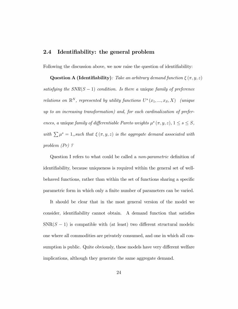
2.4 Identifiability: the general problem
Following the discussion above, we now raise the question of identifiability:
Question A (Identifiability): Take an arbitrary demand function ξ (π, y, z)
satisfying the SNR(S − 1) condition. Is there a unique family of preference
relations on RN , represented by utility functions U s (x1, ..., xS,X) (unique
up to an increasing transformation) and, for each cardinalization of prefer-
ences, a unique family of differentiable Pareto weights µs (π, y, z), 1 ≤ s ≤ S,
withPµs = 1,,such that ξ (π, y, z) is the aggregate demand associated with
problem (Pr) ?
Question I refers to what could be called a non-parametric definition of
identifiability, because uniqueness is required within the general set of well-
behaved functions, rather than within the set of functions sharing a specific
parametric form in which only a finite number of parameters can be varied.
It should be clear that in the most general version of the model we
consider, identifiability cannot obtain. A demand function that satisfies
SNR(S − 1) is compatible with (at least) two different structural models:
one where all commodities are privately consumed, and one in which all con-
sumption is public. Quite obviously, these models have very different welfare
implications, although they generate the same aggregate demand.
24

This suggests that more specific assumptions are needed. In what follows,
we assume that each commodity is either known to be privately consumed or
known to be publicly consumed. Also, preferences are egoistic in the sense
defined above. While these assumptions are natural, we shall actually see
that they are not sufficient. The nature of the indeterminacy is deeper than
suggested by the previous remark. Even with egoistic preferences - and, as a
matter of fact, even when consumptions are assumed to be either all public
or alternatively all private - it is still the case that a continuum of different
structural models generate the same group demand function. In other words,
identifying restrictions are needed, that go beyond egoistic preferences.
In the remainder of the paper, we analyze the exact nature of such restric-
tions. We first investigate the mathematical structure underlying the model.
We then prove a general result regarding uniqueness in this mathematical
framework. Finally, we derive the specific results of interest.
25
3 The mathematical structure of the identi-
fiability problem
3.1 The duality between private and public consump-
tion
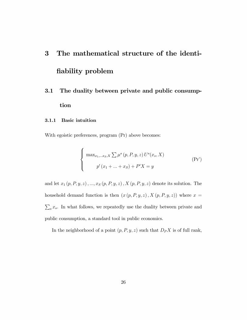
3.1.1 Basic intuition
With egoistic preferences, program (Pr) above becomes:
maxx1,...xS ,X
Pµs (p, P, y, z)Us(xs, X)
p0 (x1 + ...+ xS) + P 0X = y
(Pr’)
and let x1 (p, P, y, z) , ..., xS (p, P, y, z) ,X (p, P, y, z) denote its solution. The
household demand function is then (x (p, P, y, z) ,X (p, P, y, z)) where x =Ps xs. In what follows, we repeatedly use the duality between private and
public consumption, a standard tool in public economics.
In the neighborhood of a point (p, P, y, z) such that DPX is of full rank,
26
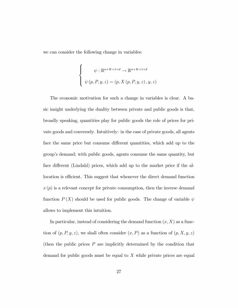
we can consider the following change in variables:
ψ : Rn+K+1+d → Rn+K+1+d
ψ (p, P, y, z) = (p,X (p, P, y, z) , y, z)
The economic motivation for such a change in variables is clear. A ba-
sic insight underlying the duality between private and public goods is that,
broadly speaking, quantities play for public goods the role of prices for pri-
vate goods and conversely. Intuitively: in the case of private goods, all agents
face the same price but consume different quantities, which add up to the
group’s demand; with public goods, agents consume the same quantity, but
face different (Lindahl) prices, which add up to the market price if the al-
location is efficient. This suggest that whenever the direct demand function
x (p) is a relevant concept for private consumption, then the inverse demand
function P (X) should be used for public goods. The change of variable ψ
allows to implement this intuition.
In particular, instead of considering the demand function (x,X) as a func-
tion of (p, P, y, z), we shall often consider (x, P ) as a function of (p,X, y, z)
(then the public prices P are implicitly determined by the condition that
demand for public goods must be equal to X while private prices are equal
27
to p,income is y and distribution factors are z). While these two viewpoints
are clearly equivalent (one can switch form the first to the second and back
using the change ψ), the computations are much easier (and more natural) in
the second case. Finally, for the sake of clarity, we omit distribution factors
for the moment, and consider functions of (p,X, y) only.
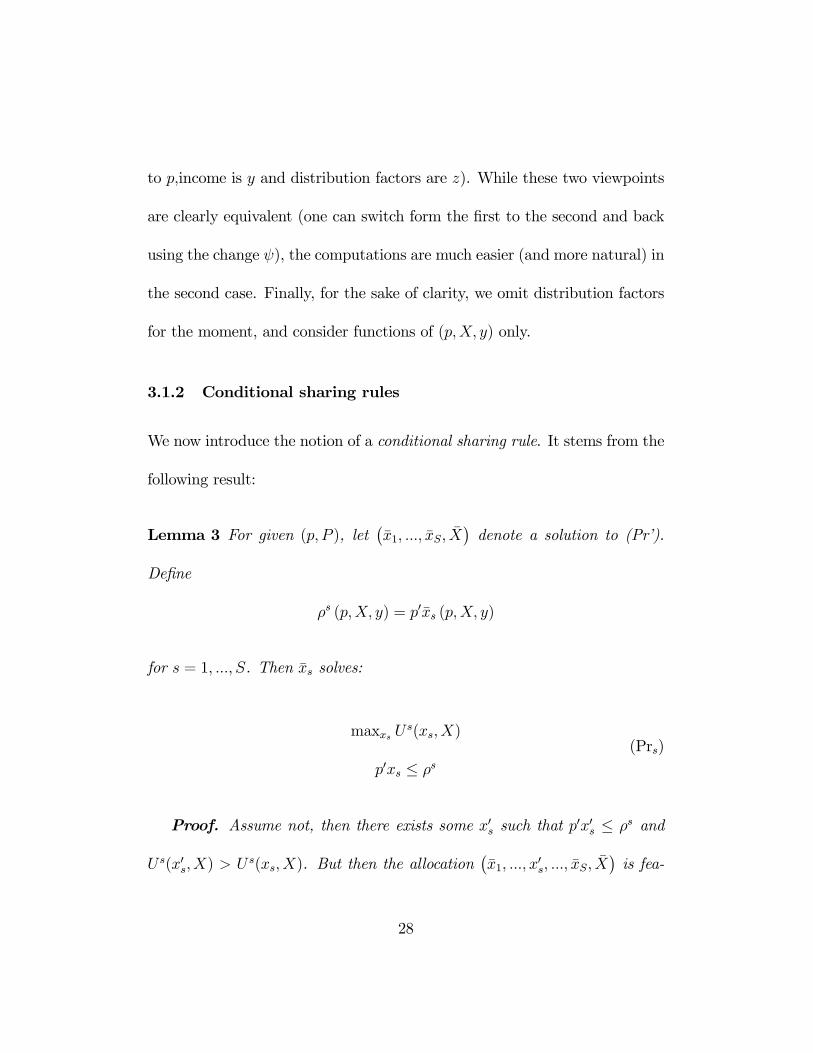
3.1.2 Conditional sharing rules
We now introduce the notion of a conditional sharing rule. It stems from the
following result:
Lemma 3 For given (p, P ), let¡x1, ..., xS, X
¢denote a solution to (Pr’).
Define
ρs (p,X, y) = p0xs (p,X, y)
for s = 1, ..., S. Then xs solves:
maxxs Us(xs,X)
p0xs ≤ ρs(Prs)
Proof. Assume not, then there exists some x0s such that p0x0s ≤ ρs and
Us(x0s,X) > Us(xs, X). But then the allocation
¡x1, ..., x
0s, ..., xS, X
¢is fea-
28

sible and Pareto dominates¡x1, ..., xS, X
¢, a contradiction.
In words, an efficient allocation can always be seen as stemming from a
two stage decision process9. At stage 1, members decide on the public pur-
chasesX, and on the allocation of the remaining income y−P 0X between the
members; member s receives ρs. At stage 2, agents each chose their vector
of private consumption, subject to their own budget constraint and taking
the level of public consumption as given. The conditional sharing rule is
the vector (ρ1, ..., ρS); it generalizes the notion of sharing rule developed in
collective models with private goods only (see for instance Chiappori (1992))
because it is defined conditionally on the level of public consumption pre-
viously chosen. Of course, if all commodities are private (K = 0) then the
conditional sharing rule boils down to the standard notion. In all cases, it
satisfies the budget constraint
Xs
ρs = y − P 0X. (2)
9Needless to say, we are not assuming that the actual decision process is in two stages.The result simply states that any efficient group behaves as if it was following a processof this type.
29
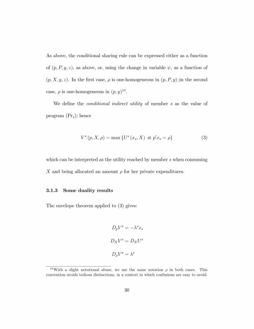
As above, the conditional sharing rule can be expressed either as a function
of (p, P, y, z), as above, or, using the change in variable ψ, as a function of
(p,X, y, z). In the first case, ρ is one-homogeneous in (p, P, y) ;in the second
case, ρ is one-homogeneous in (p, y)10.
We define the conditional indirect utility of member s as the value of
program (Prs); hence
V s (p,X, ρ) = max Us (xs, X) st p0xs = ρ (3)
which can be interpreted as the utility reached by member s when consuming
X and being allocated an amount ρ for her private expenditures.
3.1.3 Some duality results
The envelope theorem applied to (3) gives:
DpVs = −λsxs
DXVs = DXU
s
DρVs = λs
10With a slight notational abuse, we use the same notation ρ in both cases. Thisconvention avoids tedious distinctions, in a context in which confusions are easy to avoid.
30

where λs denotes the Lagrange multiplier of the budget constraint (or equiv-
alently the marginal utility of private income for member s) in (3), and where
DpV =
∂V∂p1
...
∂V∂pn
, DXV =
∂V∂X1
...
∂V∂XK
, DρV =∂V
∂ρ
Hence we have a direct extension of Roy’s identity:
DpVs
DρV s= −xs
The first stage decision process can then be modelled as:
maxX,ρ1,...,ρSP
s µs (p, P, y)V s (p,X, ρs)P
s ρs + P 0X = y
First order conditions give:
µsDρVs (p,X, ρs) = γ (p, P, y) , s = 1, ..., SX
s
µsDXVs (p,X, ρs) = γ (p, P, y)P
31
where γ denotes the Lagrange multiplier of the constraint. Setting γs = µs/γ,
we have that
DρVs (p,X, ρs) =
1
γs (p, P, y), s = 1, ..., S
which expresses the fact that individual marginal utilities of private incomes,
DρVs (p,X, ρs), are inversely proportional to Pareto weights. Finally, we
have the following conditions:
Xs
γs (p, P, y)DpVs = −
Xs
xs = −x (4)
Xs
γs (p, P, y)DXVs = P
which determine x (p, P, y) and X (p, P, y). Using the change in variable ψ,
we see that (x, P ), as a function of (p,X), can be decomposed as a linear
combination of the partial derivatives of the V s. The nice symmetry of these
equations illustrates the duality between private and public consumptions.
3.2 Collective indirect utility
Following Chiappori (2006), we introduce the following, key definition:
32

Definition 4 Given a conditional sharing rule ρs (p,X, y), the collective in-
direct utility of agent s is defined by:
W s (p,X, y) = V s (p,X, ρs (p,X, y))
In words, W s denotes the utility level reached by agent s, at prices p
and with total income y, in an efficient allocation such that the household
demand for public goods is X, taking into account the conditional sharing
rule ρs (p,X, y). Note thatW s depends not only on the preferences of agent s
(through the conditional indirect utility V s) but also on the decision process
(through the conditional sharing rule ρs). Hence W s summarizes the impact
on s of the interactions taking place within the group. As such, it is the main
concept required for welfare analysis: knowing the W s allows to assess the
impact of any reform (i.e. any change in prices and incomes) on the welfare
of each group member.
Most of what follows is devoted to the identification of the collective
indirect utility of each member.
33

3.3 Identifying collective indirect utilities : the math-
ematical structure
Condition (4) can readily be translated in terms of collective indirect utilities.
Since:
DpWs
DρV s= γsDpW
s = γsDpVs +Dpρ
s = −xs +Dpρs
DXWs
DρV s= γsDXW
s = γsDXVs +DXρ
s
DyWs
DρV s= γsDyW
s = Dyρs
and using the budget constraint (2), we conclude that:
Xs
γsDpWs = −x− (DpP )X
Xs
γsDXWs = − (DXP )X
Xs
γsDyWs = 1− (DyP )0X
Let A (p,X, y) = P (p,X, y)0X denote household total expenditures on
34
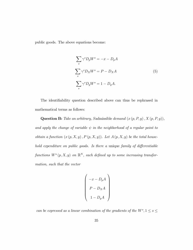
public goods. The above equations become:
Xs
γsDpWs = −x−DpA
Xs
γsDXWs = P −DXA (5)
Xs
γsDyWs = 1−DyA.
The identifiability question described above can thus be rephrased in
mathematical terms as follows:
Question B: Take an arbitrary, Sadmissible demand (x (p, P, y) , X (p, P, y)),
and apply the change of variable ψ in the neighborhood of a regular point to
obtain a function (x (p,X, y) , P (p,X, y)). Let A (p,X, y) be the total house-
hold expenditure on public goods. Is there a unique family of differentiable
functions W s (p,X, y) on RN , each defined up to some increasing transfor-
mation, such that the vector
−x−DpA
P −DXA
1−DyA
can be expressed as a linear combination of the gradients of the W s, 1 ≤ s ≤
35
S?
Decomposing a given function as a linear combination of gradients is an
old problem in mathematics, to which much work has been devoted in the
first half of the XXth century, particularly by Elie Cartan, who developed
exterior differential calculus for that purpose (among others). We shall use
these tools in what follows.
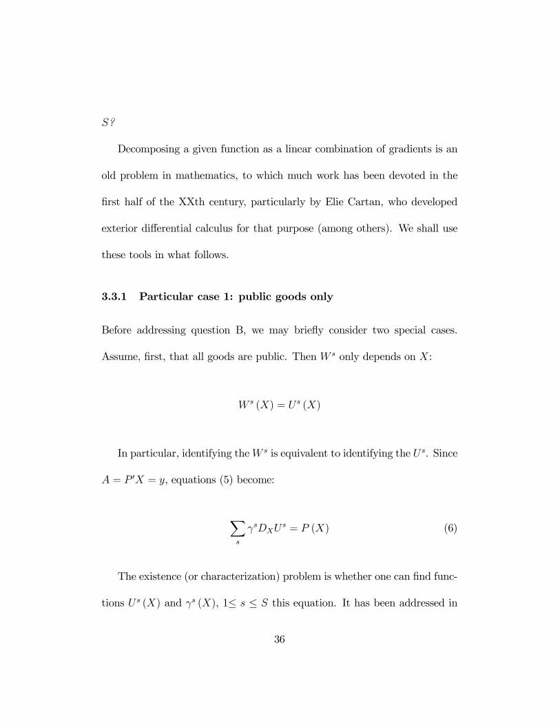
3.3.1 Particular case 1: public goods only
Before addressing question B, we may briefly consider two special cases.
Assume, first, that all goods are public. Then W s only depends on X:
W s (X) = Us (X)
In particular, identifying theW s is equivalent to identifying the Us. Since
A = P 0X = y, equations (5) become:
Xs
γsDXUs = P (X) (6)
The existence (or characterization) problem is whether one can find func-
tions U s (X) and γs (X), 1≤ s ≤ S this equation. It has been addressed in
36
Chiappori and Ekeland (2006). Here we are interested in the uniqueness (or
identification) question: are the Us (X) unique, up to an increasing transfor-
mation ?
3.3.2 Particular case 2: private goods only
The opposite polar case obtains when all commodities are private. This
is a case that has been repeatedly studied in the literature, starting with
Chiappori (1988, 1992). Then A = 0, and W s is a function of (p, y) only.
Moreover, W s, as V s, is zero-homogeneous, so we can normalize y to be one.
Equations (5) become:
Xs
γs (p)DpWs = −x (p) (7)
Remember that W s is not identical to the standard indirect utility func-
tion V s; the difference, indeed, is that W s captures both the preferences
of agent s (through V s) and the decision process (which, in that case, is
fully summarized by the sharing rule ρ). In particular, identifying W s is not
equivalent to identifying V s (hence Us).
For any given functionsW s, there exist a continuum of choices for the V s
37
and ρs, since the latter must only satisfy (using homogeneity of V s):
W s (p) = V s (p, ρs (p)) = V sµ
p
ρs (p)
¶(8)
It is easy to prove that, taking W s as given, for any ρ that is not one
homogeneous, one can locally construct a V s such that (8) is satisfied. We
conclude that, in contrast with the public good case, the knowledge of the
collective indirect utilities is not sufficient under private consumption to iden-
tify preferences and the decision process (as summarized by the sharing rule).
This indeterminacy is a direct generalization of a previous result derived by
Chiappori (1992) in a three commodity, labor supply setting.
The crucial remark, however, is that this indeterminacy is welfare irrele-
vant. If¡V 1, ..., V S; ρ1, ..., ρS
¢is a particular solution, the various, alternative
solutions¡V 1, ..., V S; ρ1, ..., ρS
¢have a very simple interpretation in welfare
terms. Namely, the V s are such that the (ordinal) utility of each member
s, when facing the sharing rule ρ, is always the same as under the V and¡ρ1, ..., ρS
¢. It follows, in particular, that any reform that is found to increase
the welfare of member s for V s and ρs will also increase her welfare for V s
and ρs. Again, identifying the collective indirect utilities W s is sufficient for
38

welfare analysis. This remark is general, and applies to any context, whatever
the number of private and public goods.
Finally, in the pure private good case, not only is the indeterminacy wel-
fare irrelevant, but it is also behavior irrelevant; i.e., two households with the
same collective indirect utilities W s and the same weights γs will exhibit the
same market behavior, irrespective of the particular sharing rule (although
intrahousehold allocation will obviously differ). Hence estimation of collec-
tive indirect utilities and weights allows to predict household behavior and
derive comparative statics conclusions.
Both equations (6) and (7) have the same mathematical structure: a given
function has to be equal to a linear combination of gradients. Necessary con-
ditions for this to happen have been recalled in Section 2. In what follows,
we first consider the identifiability problem from a mathematical perspec-
tive, then derive the corresponding economic conclusions. For expositional
convenience, Sections 4, 5 and 6 exclusively consider the case of two-person
groups (S = 2). The general case is discussed in Section 7.
39
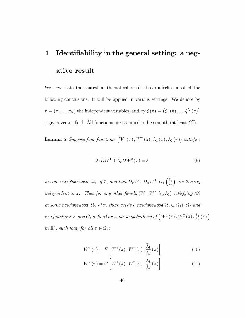
4 Identifiability in the general setting: a neg-
ative result
We now state the central mathematical result that underlies most of the
following conclusions. It will be applied in various settings. We denote by
π = (π1, ...,πN) the independent variables, and by ξ (π) =¡ξ1 (π) , ..., ξN (π)
¢a given vector field. All functions are assumed to be smooth (at least C2).
Lemma 5 Suppose four functions¡W 1 (π) , W 2 (π) , λ1 (π) , λ2 (π)
¢satisfy :
λ1DW 1 + λ2DW2 (π) = ξ (9)
in some neighborhood Ω1 of π, and that DπW1,DπW
2, Dπ
³λ1λ2
´are linearly
independent at π. Then for any other family (W 1,W 2,λ1,λ2) satisfying (9)
in some neighborhood Ω2 of π, there exists a neighborhood Ω3 ⊂ Ω1∩Ω2 and
two functions F and G, defined on some neighborhood of³W 1 (π) , W 2 (π) , λ1
λ2(π)´
in R3, such that, for all π ∈ Ω3:
W 1 (π) = F
·W 1 (π) , W 2 (π) ,
λ1λ2(π)
¸(10)
W 2 (π) = G
·W 1 (π) , W 2 (π) ,
λ1λ2(π)
¸(11)
40
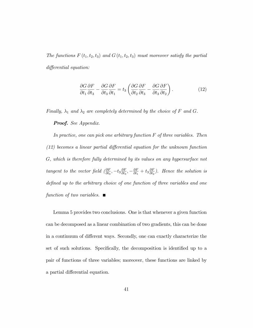
The functions F (t1, t2, t3) and G (t1, t2, t3) must moreover satisfy the partial
differential equation:
∂G
∂t1
∂F
∂t3− ∂G
∂t3
∂F
∂t1= t3
µ∂G
∂t2
∂F
∂t3− ∂G
∂t3
∂F
∂t2
¶. (12)
Finally, λ1 and λ2 are completely determined by the choice of F and G.
Proof. See Appendix.
In practice, one can pick one arbitrary function F of three variables. Then
(12) becomes a linear partial differential equation for the unknown function
G, which is therefore fully determined by its values on any hypersurface not
tangent to the vector field ( ∂F∂t3,−t3 ∂F∂t3 ,− ∂F
∂t1+ t3
∂F∂t2). Hence the solution is
defined up to the arbitrary choice of one function of three variables and one
function of two variables.
Lemma 5 provides two conclusions. One is that whenever a given function
can be decomposed as a linear combination of two gradients, this can be done
in a continuum of different ways. Secondly, one can exactly characterize the
set of such solutions. Specifically, the decomposition is identified up to a
pair of functions of three variables; moreover, these functions are linked by
a partial differential equation.
41
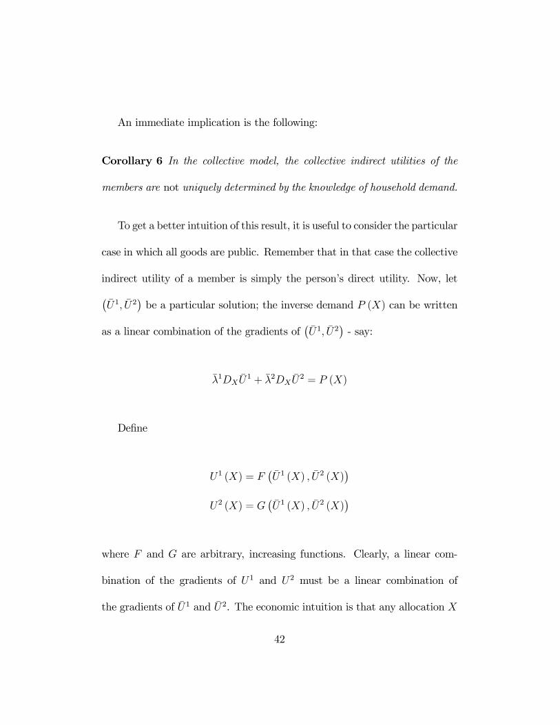
An immediate implication is the following:
Corollary 6 In the collective model, the collective indirect utilities of the
members are not uniquely determined by the knowledge of household demand.
To get a better intuition of this result, it is useful to consider the particular
case in which all goods are public. Remember that in that case the collective
indirect utility of a member is simply the person’s direct utility. Now, let¡U1, U2
¢be a particular solution; the inverse demand P (X) can be written
as a linear combination of the gradients of¡U1, U2
¢- say:
λ1DXU1 + λ2DXU
2 = P (X)
Define
U1 (X) = F¡U1 (X) , U2 (X)
¢U2 (X) = G
¡U1 (X) , U2 (X)
¢
where F and G are arbitrary, increasing functions. Clearly, a linear com-
bination of the gradients of U1 and U2 must be a linear combination of
the gradients of U1 and U2. The economic intuition is that any allocation X
42
which is Pareto efficient for (U1, U2)must also be Pareto efficient for¡U1, U2
¢(otherwise it would be possible to increase both U1 and U2, but this would
increase U1 and U2 as well, a contradiction). This gives a first intuition why
the Pareto efficiency assumption is not sufficient to distinguish between the
two solutions: if a demand function can be collectively rationalized by a cou-
ple with utilities¡U1, U2
¢then it can also be collectively rationalized by a
couple with utilities¡F¡U1, U2
¢, G¡U1, U2
¢¢.
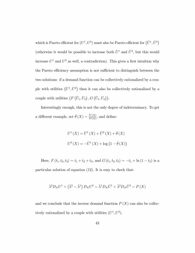
Interestingly enough, this is not the only degree of indeterminacy. To get
a different example, set θ (X) = λ1(X)
λ2(X), and define:
U1 (X) = U1 (X) + U2 (X) + θ (X)
U2 (X) = −U1 (X) + log ¡1− θ (X)¢
Here, F (t1, t2, t3) = t1 + t2 + t3, and G (t1, t2, t3) = −t1 + ln (1− t3) is a
particular solution of equation (12). It is easy to check that:
λ2DXU1 +
¡λ2 − λ1
¢DXU
2 = λ1DXU1 + λ2DXU
2 = P (X)
and we conclude that the inverse demand function P (X) can also be collec-
tively rationalized by a couple with utilities (U1, U2).
43
5 Identifiability under exclusivity
The previous section concludes that identifiability does not obtain in the
general version of the collective model. The next step is to find specific,
additional assumptions that guarantee identifiability. We now show that a
simple exclusivity condition is sufficient in general.
5.1 The main result
Again, suppose four functions¡W 1 (π) , W 2 (π) , λ1 (π) , λ2 (π)
¢satisfy equa-
tion (9) in some neighborhood Ω1 of π. We shall say that this solution is
generic if DπW1, DπW
2 and Dπθ are linearly independent at π, and
∂W 2
∂π1(π) 6= 0 and Da,b,c,d (π) 6= 0 for some a, b, c, d ∈ 1, ..., N (13)
44
where:
θ (π) =λ1 (π)
λ2 (π), Φ (π) =
∂θ
∂π1(π)
·∂W 2
∂π1(π)
¸−1(14)
Da,b,c,d =
¯¯¯¯
∂Φ∂πa
∂W 1
∂πa∂W 2
∂πa∂θ∂πa
∂Φ∂πb
∂W 1
∂πb
∂W 2
∂πb
∂θ∂πb
∂Φ∂πc
∂W 1
∂πc∂W 2
∂πc∂θ∂πc
∂Φ∂πd
∂W 1
∂πd
∂W 2
∂πd
∂θ∂πd
¯¯¯¯
(15)
Note that if equations (13) hold at π, they will hold in a neihgborhood of
π as well. Note also that in a practical situation, there is no reason to expect
that the functions W 1, W 2 and θ = λ1/λ2 would satisfy these equations, and
if they do, a slight perturbation of the model would ensure that they do not.
We shall say that W 1is exclusive in Ω if:
∂W 1
∂π1(π) = 0 ∀π ∈ Ω (16)
We now show that exclusivity is sufficient to guarantee identifiability
for generic models. Note, first, that the result is obvious if the number
of commodities is exactly 2 - since individual consumptions are perfectly
observed in that case. Also, the case N = 3 has been already solved by
45
Chiappori (1992) for private goods and Blundell et al. (2006) for public
goods. We are thus left with the general case N ≥ 4. The main result is the
following:
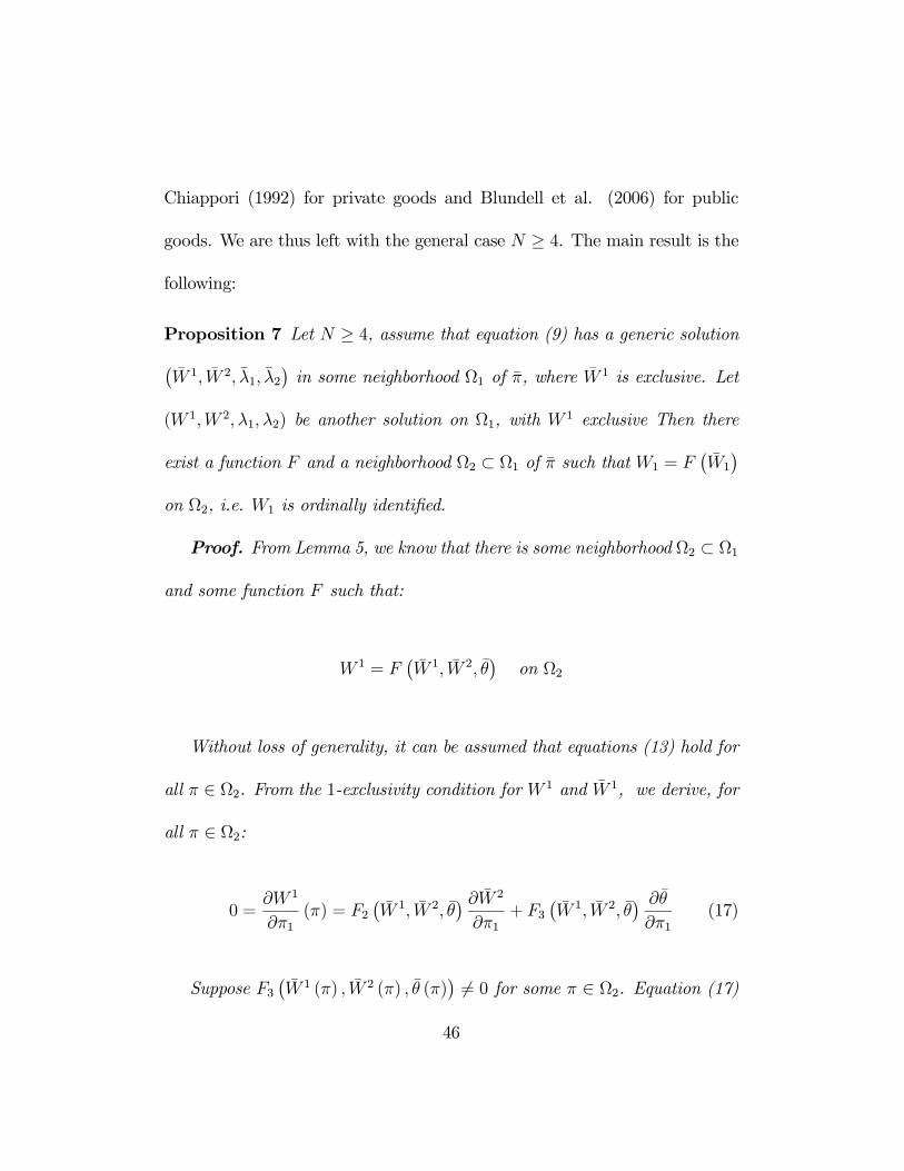
Proposition 7 Let N ≥ 4, assume that equation (9) has a generic solution¡W 1, W 2, λ1, λ2
¢in some neighborhood Ω1 of π, where W 1 is exclusive. Let
(W 1,W 2,λ1,λ2) be another solution on Ω1, with W 1 exclusive Then there
exist a function F and a neighborhood Ω2 ⊂ Ω1 of π such that W1 = F¡W1
¢on Ω2, i.e. W1 is ordinally identified.
Proof. From Lemma 5, we know that there is some neighborhood Ω2 ⊂ Ω1
and some function F such that:
W 1 = F¡W 1, W 2, θ
¢on Ω2
Without loss of generality, it can be assumed that equations (13) hold for
all π ∈ Ω2. From the 1-exclusivity condition for W 1 and W 1, we derive, for
all π ∈ Ω2:
0 =∂W 1
∂π1(π) = F2
¡W 1, W 2, θ
¢ ∂W 2
∂π1+ F3
¡W 1, W 2, θ
¢ ∂θ
∂π1(17)
Suppose F3¡W 1 (π) , W 2 (π) , θ (π)
¢ 6= 0 for some π ∈ Ω2. Equation (17)
46
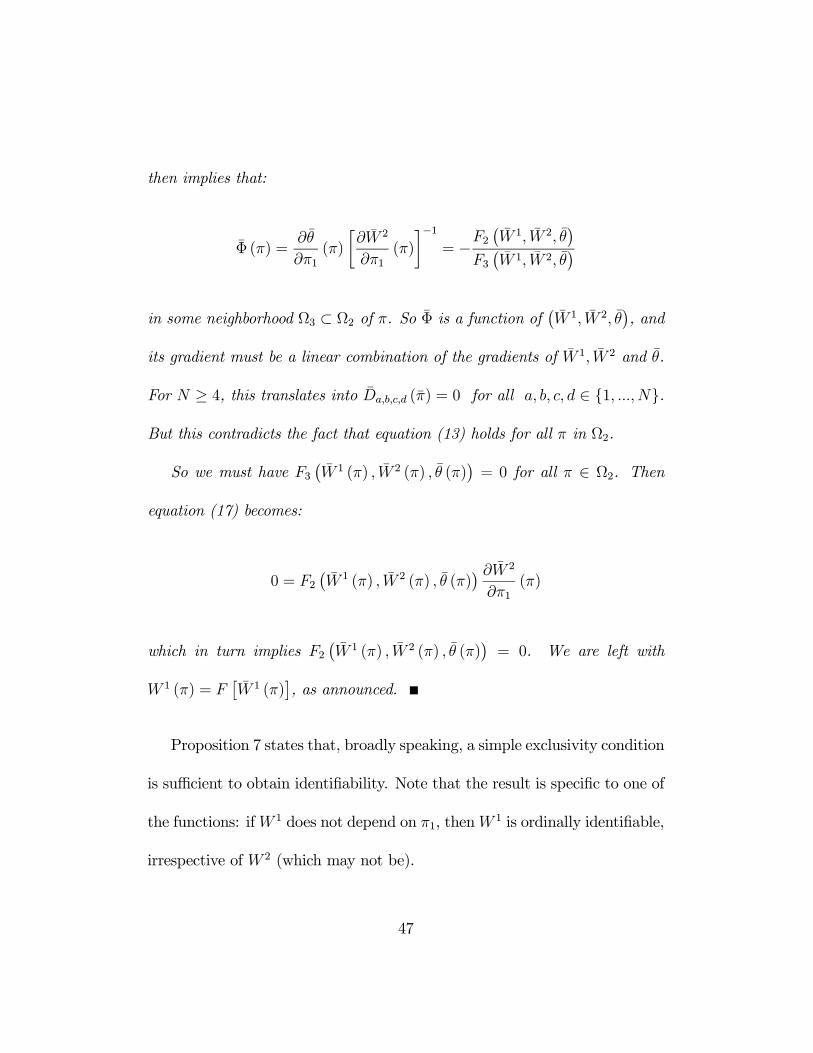
then implies that:
Φ (π) =∂θ
∂π1(π)
·∂W 2
∂π1(π)
¸−1= −F2
¡W 1, W 2, θ
¢F3¡W 1, W 2, θ
¢in some neighborhood Ω3 ⊂ Ω2 of π. So Φ is a function of
¡W 1, W 2, θ
¢, and
its gradient must be a linear combination of the gradients of W 1, W 2 and θ.
For N ≥ 4, this translates into Da,b,c,d (π) = 0 for all a, b, c, d ∈ 1, ..., N.
But this contradicts the fact that equation (13) holds for all π in Ω2.
So we must have F3¡W 1 (π) , W 2 (π) , θ (π)
¢= 0 for all π ∈ Ω2. Then
equation (17) becomes:
0 = F2¡W 1 (π) , W 2 (π) , θ (π)
¢ ∂W 2
∂π1(π)
which in turn implies F2¡W 1 (π) , W 2 (π) , θ (π)
¢= 0. We are left with
W 1 (π) = F£W 1 (π)
¤, as announced.
Proposition 7 states that, broadly speaking, a simple exclusivity condition
is sufficient to obtain identifiability. Note that the result is specific to one of
the functions: ifW 1 does not depend on π1, thenW 1 is ordinally identifiable,
irrespective of W 2 (which may not be).
47
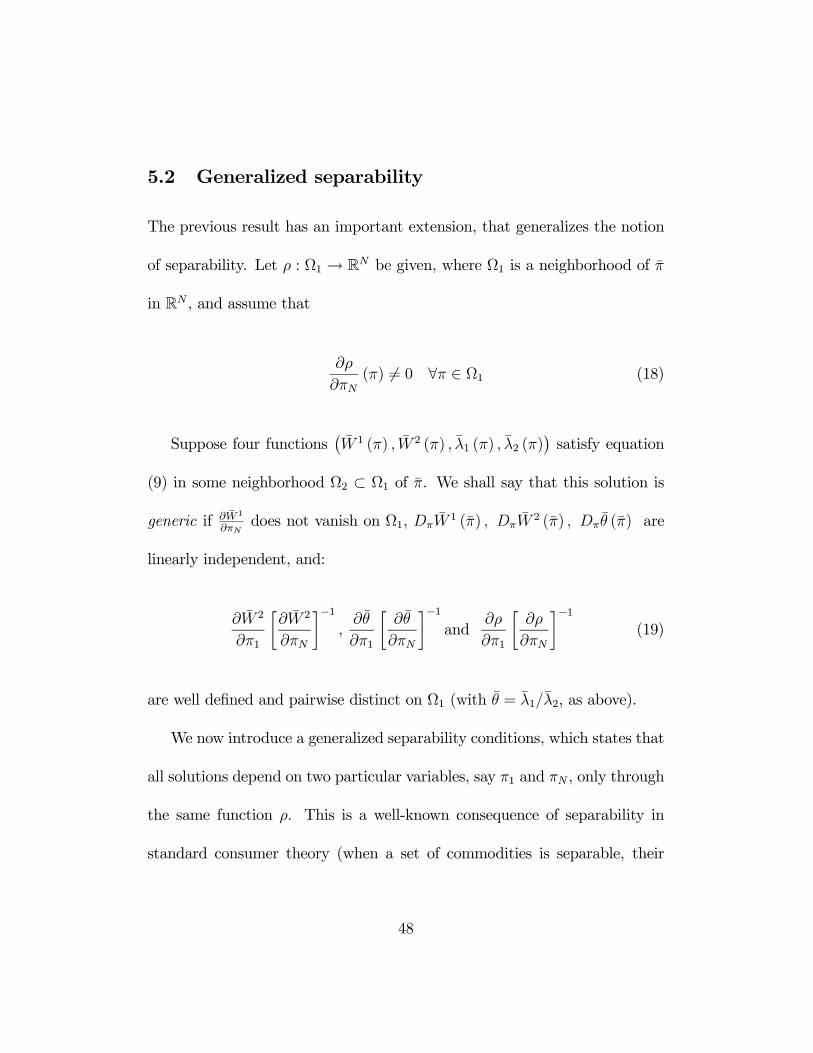
5.2 Generalized separability
The previous result has an important extension, that generalizes the notion
of separability. Let ρ : Ω1 → RN be given, where Ω1 is a neighborhood of π
in RN , and assume that
∂ρ
∂πN(π) 6= 0 ∀π ∈ Ω1 (18)
Suppose four functions¡W 1 (π) , W 2 (π) , λ1 (π) , λ2 (π)
¢satisfy equation
(9) in some neighborhood Ω2 ⊂ Ω1 of π. We shall say that this solution is
generic if ∂W 1
∂πNdoes not vanish on Ω1, DπW
1 (π) , DπW2 (π) , Dπθ (π) are
linearly independent, and:
∂W 2
∂π1
·∂W 2
∂πN
¸−1,∂θ
∂π1
·∂θ
∂πN
¸−1and
∂ρ
∂π1
·∂ρ
∂πN
¸−1(19)
are well defined and pairwise distinct on Ω1 (with θ = λ1/λ2, as above).
We now introduce a generalized separability conditions, which states that
all solutions depend on two particular variables, say π1 and πN , only through
the same function ρ. This is a well-known consequence of separability in
standard consumer theory (when a set of commodities is separable, their
48
demand depends on the other prices only through an income effect), which
explains the expression ‘generalized separability’.
Technically, let ρ be a given, smooth function. We shall say that W 1 is
separable for ρ if:
∂ρ
∂πN(π)
∂W 1
∂π1(π) =
∂W 1
∂πN(π)
∂ρ
∂π1(π) (20)
Corollary 8 Let N ≥ 4. Assume that ¡W 1, W 2, λ1, λ2¢is a generic solution
of equation (9)on Ω2 and that W 1 is separable for ρ. Let (W 1,W 2,λ1,λ2) be
another solution on Ω2, with W 1 separable for the same ρ. Then there exist
a function F and a neighborhood Ω3 ⊂ Ω2 of π such that W1 = F¡W1
¢on
Ω3, i.e. W1 is ordinally identified.
Proof. We claim that W 1 can be written under the form:
W 1 (π) = K1 [π2, ...,πN−1, ρ (π)] (21)
Indeed, the map:
(π1,π2, ...,πN)→ (π1,π2, ...,πN−1, ρ (π)) (22)
49
is invertible in a neighborhood Ω3 of π by condition (18). So W 1 can be
written as:
W 1 (π) = K1 [π1,π2, ...,πN−1, ρ (π)]
Differentiating, we get:
∂W 1
∂π1=
∂K1
∂π1+
∂K1
∂ρ
∂ρ
∂π1
∂W 1
∂πN=
∂K1
∂ρ
∂ρ
∂πN
∂W 1
∂π1
·∂W 1
∂πN
¸−1=
∂K1
∂π1
·∂K1
∂ρ
∂ρ
∂πN
¸−1+
∂ρ
∂π1
·∂ρ
∂πN
¸−1
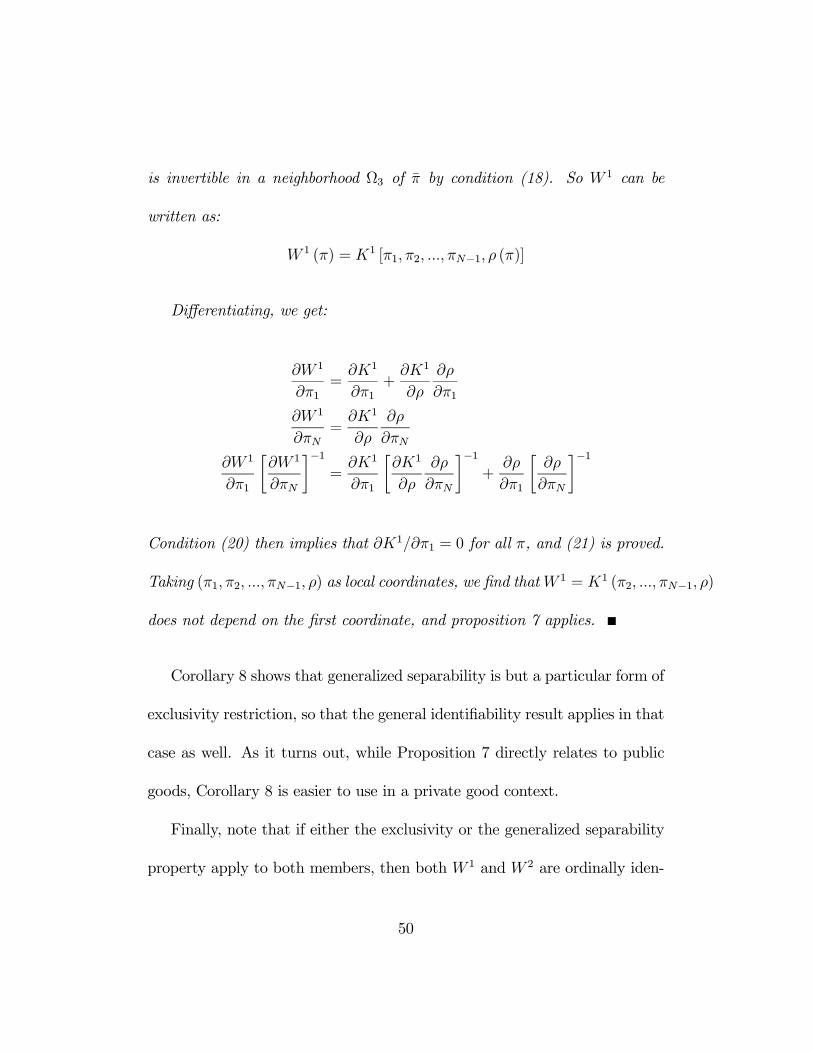
Condition (20) then implies that ∂K1/∂π1 = 0 for all π, and (21) is proved.
Taking (π1,π2, ...,πN−1, ρ) as local coordinates, we find thatW 1 = K1 (π2, ...,πN−1, ρ)
does not depend on the first coordinate, and proposition 7 applies.
Corollary 8 shows that generalized separability is but a particular form of
exclusivity restriction, so that the general identifiability result applies in that
case as well. As it turns out, while Proposition 7 directly relates to public
goods, Corollary 8 is easier to use in a private good context.
Finally, note that if either the exclusivity or the generalized separability
property apply to both members, then both W 1 and W 2 are ordinally iden-
50
tifiable. Then for any cardinalization of W 1 and W 2, the coefficients λi are
identifiable as well.
5.3 The meaning of genericity.
Before discussing the economic interpretation of the previous results, a re-
mark is in order. In Proposition 7 and Corollary 8, identifiability is only
‘generic’. Technically, what Proposition 7 shows is that identifiability obtains
unless the structural functions W 1, W 2, θ satisfy a set of partial differential
equations that can be explicitly derived. It is thus important to understand
the exact scope of these partial differential equations, and particularly to
discuss examples in which they are satisfied everywhere.
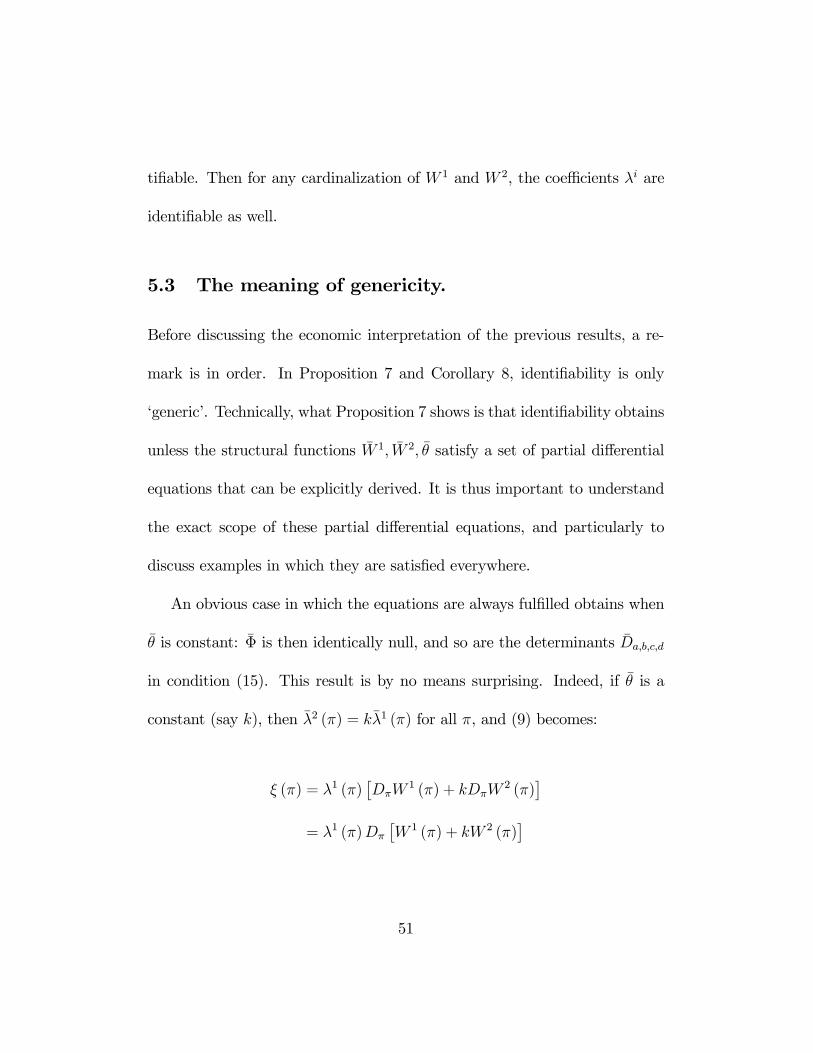
An obvious case in which the equations are always fulfilled obtains when
θ is constant: Φ is then identically null, and so are the determinants Da,b,c,d
in condition (15). This result is by no means surprising. Indeed, if θ is a
constant (say k), then λ2 (π) = kλ1 (π) for all π, and (9) becomes:
ξ (π) = λ1 (π)£DπW
1 (π) + kDπW2 (π)
¤= λ1 (π)Dπ
£W 1 (π) + kW 2 (π)
¤
51
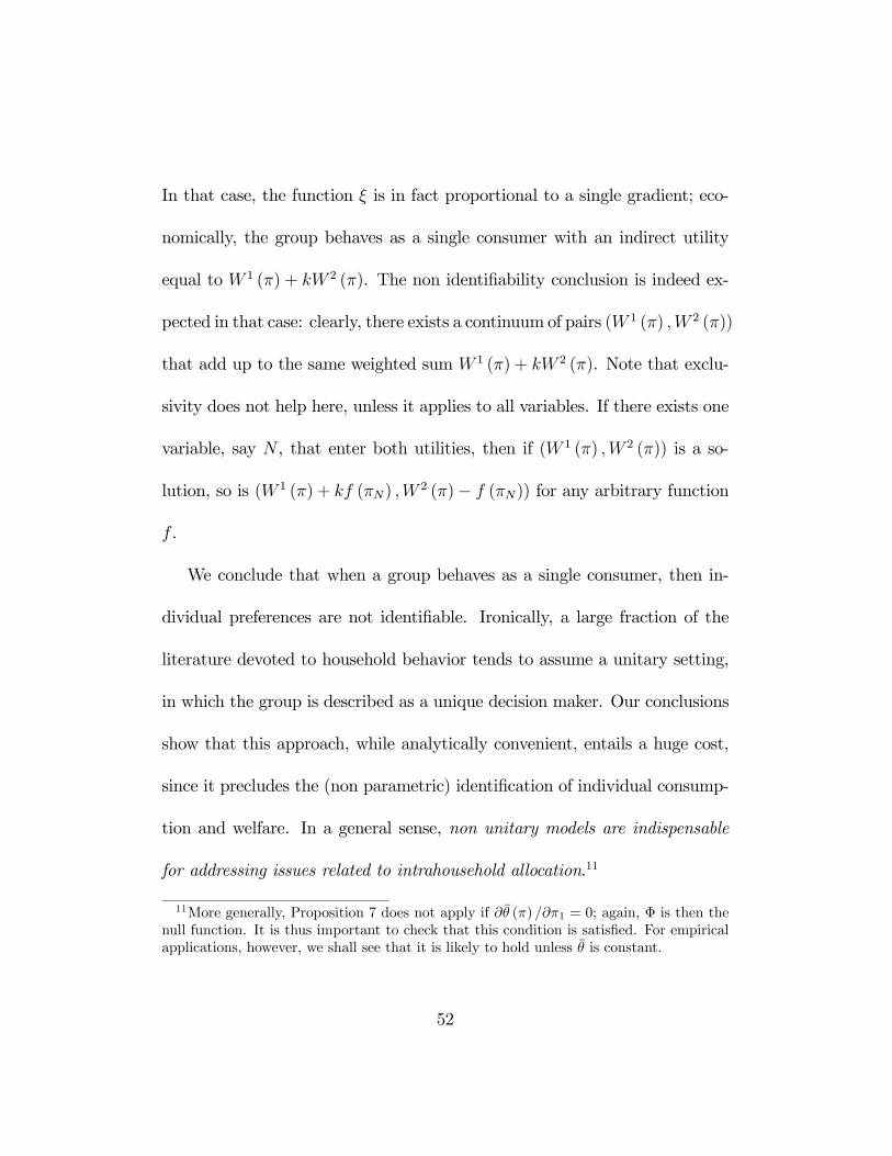
In that case, the function ξ is in fact proportional to a single gradient; eco-
nomically, the group behaves as a single consumer with an indirect utility
equal to W 1 (π) + kW 2 (π). The non identifiability conclusion is indeed ex-
pected in that case: clearly, there exists a continuum of pairs (W 1 (π) ,W 2 (π))
that add up to the same weighted sum W 1 (π) + kW 2 (π). Note that exclu-
sivity does not help here, unless it applies to all variables. If there exists one
variable, say N , that enter both utilities, then if (W 1 (π) ,W 2 (π)) is a so-
lution, so is (W 1 (π) + kf (πN) ,W2 (π)− f (πN)) for any arbitrary function
f .
We conclude that when a group behaves as a single consumer, then in-
dividual preferences are not identifiable. Ironically, a large fraction of the
literature devoted to household behavior tends to assume a unitary setting,
in which the group is described as a unique decision maker. Our conclusions
show that this approach, while analytically convenient, entails a huge cost,
since it precludes the (non parametric) identification of individual consump-
tion and welfare. In a general sense, non unitary models are indispensable
for addressing issues related to intrahousehold allocation.11
11More generally, Proposition 7 does not apply if ∂θ (π) /∂π1 = 0; again, Φ is then thenull function. It is thus important to check that this condition is satisfied. For empiricalapplications, however, we shall see that it is likely to hold unless θ is constant.
52
Finally, except for these particular cases, the identifiability result is quite
robust. It is easy to check, for instance, that whenever a particular solution¡W 1, W 2, θ
¢is non-generic, so so that the equations (??) and (13) are satis-
fied, the property is not robust to slight perturbations of either preferences
or weights. Consider, for instance, linear versions of all functions:
λ1 (π) =Xi
λ1iπi, λ2 (π) =
Xi
λ2iπi
so that:
θ (π) =
Pi λ
1iπiP
i λ2iπi, W 1 (π) =
Xi
w1i πi, W2 (π) =
Xi
w2i πi
Assume that the conditions (16) are satisfied:
w11 = 0, w21 6= 0,
Xi
¡λ11λ
2i − λ21λ
1i
¢πi 6= 0
(note that the last inequality is satisfied whenever one at least of the (λ11λ2i − λ21λ
1i )
is non zero - i.e., whenever λ1 and λ2 are not proportional).
Then
Φ (π) =∂θ/∂π1∂W 2/∂π1
=
Pi (λ
11λ2i − λ21λ
1i )πi
w21 (P
i λ2iπi)
2
53
therefore
Da,b,c,d =
¯¯¯¯¯
(λ11λ2a−λ21λ1a)(Pi λ
2i πi)−2λ2a(
Pi(λ11λ2i−λ21λ1i )πi)
w21(Pi λ
2i πi)
3 w1a w2a
Pi(λ1aλ2i−λ2aλ1i )πi(Pi λ
2i πi)
2
(λ11λ2b−λ21λ1b)(Pi λ
2i πi)−2λ2b(
Pi(λ11λ2i−λ21λ1i )πi)
w21(Pi λ
2i πi)
3 w1b w2b
Pi(λ1bλ2i−λ2bλ1i )πi(Pi λ
2i πi)
2
(λ11λ2c−λ21λ1c)(Pi λ
2i πi)−2λ2c(
Pi(λ11λ2i−λ21λ1i )πi)
w21(Pi λ
2i πi)
3 w1c w2c
Pi(λ1cλ2i−λ2cλ1i )πi(Pi λ
2i πi)
2
(λ11λ2d−λ21λ1d)(Pi λ
2i πi)−2λ2d(
Pi(λ11λ2i−λ21λ1i )πi)
w21(Pi λ
2i πi)
3 w1d w2d
Pi(λ1dλ2i−λ2dλ1i )πi(Pi λ
2i πi)
2
¯¯¯¯¯
(23)
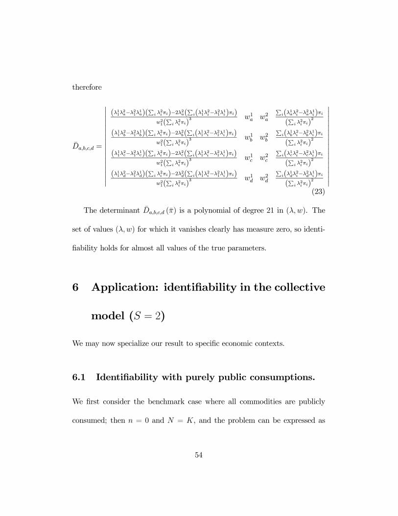
The determinant Da,b,c,d (π) is a polynomial of degree 21 in (λ, w). The
set of values (λ, w) for which it vanishes clearly has measure zero, so identi-
fiability holds for almost all values of the true parameters.
6 Application: identifiability in the collective
model (S = 2)
We may now specialize our result to specific economic contexts.
6.1 Identifiability with purely public consumptions.
We first consider the benchmark case where all commodities are publicly
consumed; then n = 0 and N = K, and the problem can be expressed as
54
(see section 3.3.1): Xs=1,2
γsDXUs = P (X, y)
where γs = µs/γ. In that case, the exclusivity assumption has a natural
translation, namely that commodity 1 (resp. 2) is exclusively consumed by
member 1 (resp. 2). We conclude from Proposition 7 that U1 and U2 are
ordinally identifiable. Moreover, for any cardinalization of these utilities,
the coefficients γs are exactly identifiable. Since they are proportional to
the Pareto weights and that the latter add up to one, we conclude that the
Pareto weights are identifiable as well. In summary:
Corollary 9 In the collective model with two agents and public consumption
only, if member 1 does not consume at least one good, then generically the
utility of member 1 is exactly (ordinally) identifiable from household demand.
If each member is the exclusive consumer of at least one good, then generi-
cally individual preferences are exactly (ordinally) identifiable from household
demand; and for any cardinalization of individual utilities, the Pareto weights
are exactly identifiable.
We may briefly discuss the conditions needed for identifiability. One is
that ∂W 2(π)∂π1
6= 0, i.e. in this case ∂U2(π)∂X1 6= 0. Clearly, if commodity one is
55
valued neither by member 1 nor by member 2, household demand for this
good is zero and cannot be used for identification.
More demanding is the requirement that ∂θ∂X1 6= 0. In our context, θ is the
ratio of individual Pareto weights. In general, Pareto weights are functions of
prices P and income y. In Proposition 7, however, θ is expressed as a function
of (X, y) to exploit the private/public goods duality. The link between the
two is straightforward: if µ denotes the ratio of Pareto weights, we have
θ (X, y) = µ [P (X, y) , y], and hence:
∂θ
∂X1=
KXk=1
∂µ
∂Pk
∂Pk∂X1
This partial ∂θ∂X1 cannot be zero unless the vector
¡∂P1∂X1 , ...,
∂PK∂X1
¢is orthog-
onal to the gradient of µ in P . This will surely occur if µ is constant, since
the gradient is null. This is the case, discussed above, in which the house-
hold behaves as a single decision maker and maximizes the unitary utility
U1+µU2. If µ is not constant, however, then ∂θ∂X1 = 0 leads to the equation:
KXk=1
∂µ
∂Pk[P (X, y) , y]
∂Pk∂X1
(X, y) = 0
56
Taking (P, y) as independent variables instead of (X, y), we get an equa-
tion of the form:KXk=1
∂µ
∂Pk(P, y)ϕk (P, y) = 0 (24)
where the ϕk, 1 ≤ k ≤ K depend on µ, U1 and U2. It can be shown that,
generically12 in (µ,U1, U2), equation (24) defines a submanifold Σ of codi-
mension 1 (and hence a set of measure 0) in RK × R. In other words, if the
actual µ,U1 and U2 are generic (in particular, if µ is not constant), there
is a set Σ of measure 0 such that, whenever (P, y) /∈ Σ, Pareto weights and
preferences can be uniquely recovered from observing the collective demand
function X (P, y) near¡P , y
¢.
6.2 Application: collective models of labor supply with
public consumptions
An immediate application is to the collective model of household labor sup-
ply, initially introduced by Chiappori (1988, 1992). The idea is to consider
12Here, genericity is taken in the sense of Thom; it means that the set N of¡µ,U1, U2
¢where the property does not hold is small in an appropriate sense. To be precise, it is, inan appropriate function space, a countable union of closed sets with empty interiors. Asa consequence, it has itself an empty interior, so that if
¡µ, U1, U2
¢happens to belong to
N , there are neighbours ¡µ,U1, U2¢, which are as close as one wishes to ¡µ, U1, U2¢ andwhich do not belong to N .
57
the household as a two-person group making Pareto efficient decisions on
consumption and labor supply; let Ls denote the leisure of member s, and ws
the corresponding wage. Various versions of the model can be considered. In
each of them Corollary 9 applies, leading to full identifiability of the model.
1. Leisure as an exclusive good
In the first model, each member’s leisure is exclusive and there is no
household production. Labor and non labor incomes are used to pur-
chase commodities X1, ..., XK that are publicly consumed within the
household; utilities are thus of the form Us¡Ls,X1, ...,XK
¢.
2. Leisures are public, one exclusive good per member
In the second model, leisure of one member is also consumed by the
other member; again, there is no household production. The identifying
assumption is that there exists two commodities (say, 1 and 2) such that
commodity i is exclusively consumed by member s.13 One can think,
for instance, of clothing as the exclusive commodity (as in Browning
et al 1994), but many other examples can be considered. Utilities
are then of the form Us¡L1, L2, Xs,X3, ...,XK
¢. Again, Proposition
13This framework is close to (but less general than) that of Fong and Zhang (2000)
58
9 applies: from the observation of the two labor supplies and the K
consumptions as functions of prices, wages and non labor income, it
is possible to uniquely recover preferences and Pareto weights. This
is a strong result indeed, since it states that one can, from the sole
observation of household labor supply and consumption, identify the
partials ∂U i/∂Lj, i 6= j, that is, deduce to what extent individual
leisures are publicly consumed.
3. Leisure as exclusive goods with household production
As a third example, assume that individual time can be devoted to
three different uses: leisure, market work and household production.
The domestic good Y is produced from domestic labor under some
constant return to scale technology, say Y = f (t1, t2),14 and pub-
licly consumed within the household. Preferences are of the form
U s¡Ls, Y,X1, ..., XK
¢and one can define
U s¡Ls, t1, t2,X1, ..., XK
¢= Us
¡Ls, f
¡t1, t2
¢,X1, ..., XK
¢(25)
Here, Y is not observable in general, but t1 and t2 are observed, which
14Other inputs can be introduced at no cost, provided they are observable.
59

typically requires data over time use (obviously, there is little chance to
identify household production if neither the output nor the input are
observable).
From Proposition 9, the Us are identified. Then the production tech-
nology can be recovered up to a scaling factor, using the assumption
of constant return to scale, from the relation:
∂U1/∂t1
∂U1/∂t2=
∂U2/∂t1
∂U2/∂t2=
∂f/∂t1
∂f/∂t2
which in addition generates an overidentifying restriction. Finally, (25)
allows to recover the Us; again, the separability property in (25) gen-
erates additional, testable restrictions.
4. Leisures are public, one exclusive good per member and house-
hold production
Finally, one can combine models 2 and 3 by assuming that leisure is
a public good, but the demand for two other exclusive goods can be
observed. Again, identifiability generically obtains in this context.
60
6.3 Identifiability in the general case
We may now address the general case with private and public consumptions,
that is, we want to solve the system of equations (5) for a given A (p,X, y).
A first remark is that a commodity exclusively consumed by a member can
arbitrarily be considered as private or public. In what follows, we adopt the
convention that such a good is always considered as private.
In the presence of private consumption, the problem is more complex,
because the exclusivity assumption of the type introduced in Proposition 7
does not have a direct economic translation. Indeed, remember that:
W s (p,X, y) = V s (p,X, ρs (p,X, y))
hence:
∂W 1
∂p1=
∂V 1
∂p1+
∂V 1
∂ρ1∂ρ1
∂p1
We see, in particular, that even when consumer 1 does not consume com-
modity 2, so that ∂V 1
∂p1= ∂U1
∂X1 = 0, we still have that ∂W 1
∂p1= ∂V 1
∂ρ∂ρ1
∂p16= 0
in general. Intuitively, even when a public good is not consumed by an
agent, the corresponding expenditures may still impact the agent’s share of
resources, therefore the agent’s welfare, through an income effect.
61
However, Corollary 8 is now the relevant tool. Take a point¡p, X, y
¢and
assume that:
∂ρ1
∂y
¡p, X, y
¢ 6= 0. (26)
From now on, all results are understood to be local, that is, to hold in
some neighborhood of¡p, X, y
¢.
Assume, now, that commodity 1 is not consumed by member 1, and
commodity 2 is not consumed by member 2:
∂V i
∂pi=
∂U i
∂X i= 0, i = 1, 2
It follows, first, that for any solution W :
∂W 1 (p,X, y) /∂p1∂W 1 (p,X, y) /∂y
=∂ρ1 (p,X, y) /∂p1∂ρ1 (p,X, y) /∂y
Let (U1, U2, ρ1, ρ2 = y −A− ρ1) and¡U1, U2, ρ1, ρ2 = y −A− ρ1
¢be the
utilities and conditional sharing rules corresponding to two different solutions
of equations (5). We have:
∂W 1/∂p1∂W 1/∂y
=∂ρ1/∂p1∂ρ1/∂y
and∂W 1/∂p1∂W 1/∂y
=∂ρ1/∂p1∂ρ1/∂y
(27)
62
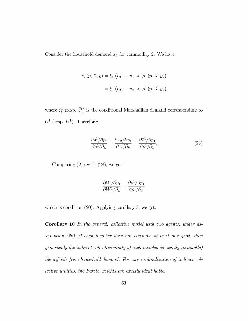
Consider the household demand x1 for commodity 2. We have:
x2 (p,X, y) = ξ12¡p2, ..., pn, X, ρ
1 (p,X, y)¢
= ξ12¡p2, ..., pn, X, ρ
1 (p,X, y)¢
where ξ1i (resp. ξ1i ) is the conditional Marshallian demand corresponding to
U1 (resp. U1). Therefore:
∂ρ1/∂p1∂ρ1/∂y
=∂x2/∂p1∂xi/∂y
=∂ρ1/∂p1∂ρ1/∂y
. (28)
Comparing (27) with (28), we get:
∂W/∂p1∂W 1/∂y
=∂ρ1/∂p1∂ρ1/∂y
which is condition (20). Applying corollary 8, we get:
Corollary 10 In the general, collective model with two agents, under as-
sumption (26), if each member does not consume at least one good, then
generically the indirect collective utility of each member is exactly (ordinally)
identifiable from household demand. For any cardinalization of indirect col-
lective utilities, the Pareto weights are exactly identifiable.
63

Note, however, that the conditions (19) have to be satisfied. Although
they hold true in a ’generic’ sense, checking that they are fulfilled in a spe-
cific context may be tedious. In such cases, using distribution factors may
facilitate identifiability (see below).
Links with the existing literature The statements derived above gen-
eralize several results existing in the literature.
1. In an earlier work, Chiappori (1992) analyzed a collective model of labor
supply in three goods framework (two labor supplies and an Hicksian
composite good). In this model, all commodities are privately con-
sumed, and each member’s labor supply is exclusive. Chiappori shows
that:
• efficiency is equivalent to the existence of a sharing rule
• the sharing rule is identifiable from labor supply up to an additive
constant; for any choice of the constant, individual preferences are
exactly identified.
• finally, the additive constant is welfare-irrelevant.
Our paper generalizes these conclusions to a general framework, in-
64
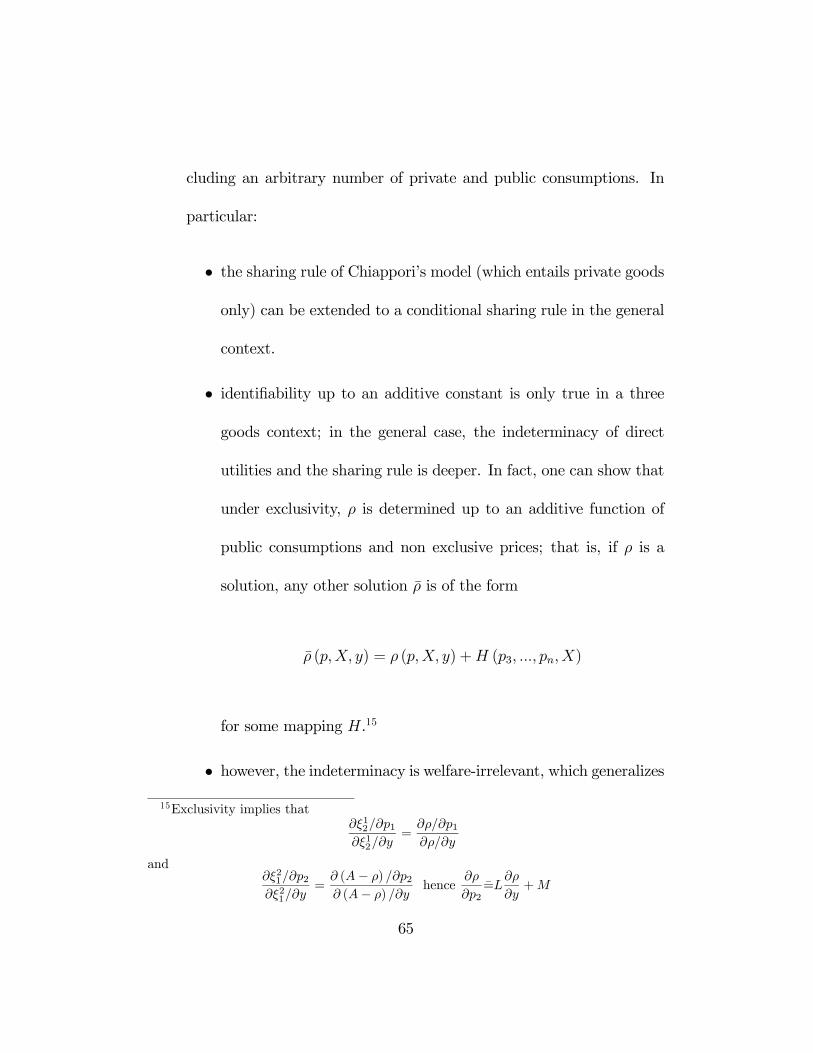
cluding an arbitrary number of private and public consumptions. In
particular:
• the sharing rule of Chiappori’s model (which entails private goods
only) can be extended to a conditional sharing rule in the general
context.
• identifiability up to an additive constant is only true in a three
goods context; in the general case, the indeterminacy of direct
utilities and the sharing rule is deeper. In fact, one can show that
under exclusivity, ρ is determined up to an additive function of
public consumptions and non exclusive prices; that is, if ρ is a
solution, any other solution ρ is of the form
ρ (p,X, y) = ρ (p,X, y) +H (p3, ..., pn, X)
for some mapping H.15
• however, the indeterminacy is welfare-irrelevant, which generalizes15Exclusivity implies that
∂ξ12/∂p1∂ξ12/∂y
=∂ρ/∂p1∂ρ/∂y
and∂ξ21/∂p2∂ξ21/∂y
=∂ (A− ρ) /∂p2∂ (A− ρ) /∂y
hence∂ρ
∂p2=L
∂ρ
∂y+M
65

Chiappori’s conclusion.
2. In a recent paper, Blundell, Chiappori and Meghir (from now on BCM)
analyze a similar model, with the difference that the non exclusive good
is public (and can be interpreted as children expenditures or welfare).
They prove that their model is generically identifiable.16 The identi-
fiability result in BCM stems directly from Corollary 9 (the model is
where
L =∂ξ21/∂p2∂ξ21/∂y
,M =∂A
∂p2− ∂ξ21/∂p2
∂ξ21/∂y
∂A
∂y
The first condition implies that for any ρ,
ρ (p,X, y) = H (ρ (p,X, y) , p2, p3, ..., pn,X)
hence∂ρ
∂p2=
∂H
∂ρ
∂ρ
∂p2+
∂H
∂p2and L
∂ρ
∂y+M = L
∂H
∂ρ
∂ρ
∂y+M
and the second becomes
∂H
∂ρ
µL∂ρ
∂y+M
¶+
∂H
∂p2= L
∂H
∂ρ
∂ρ
∂y+M
or∂H
∂p2=
µ1− ∂H
∂ρ
¶M
If ∂H∂ρ 6= 1 then
M =∂H/∂p21− ∂H/∂ρ
and the function M can be written as a function of (ρ, p2, p3, ..., pn,X). Generically, thiscannot be the case; therefore ∂H
∂ρ = 1,∂H∂p2
= 0, hence the conclusion.16BCM provide a detailed analysis of the comparative statics of such a model and of
its welfare implications. They show, in particular, that increasing the Pareto weight of aparticular member increases the household demand for a public good if and only if theperson’s marginal willingness to pay for the public good is more income sensitive thanthat of her spouse.
66
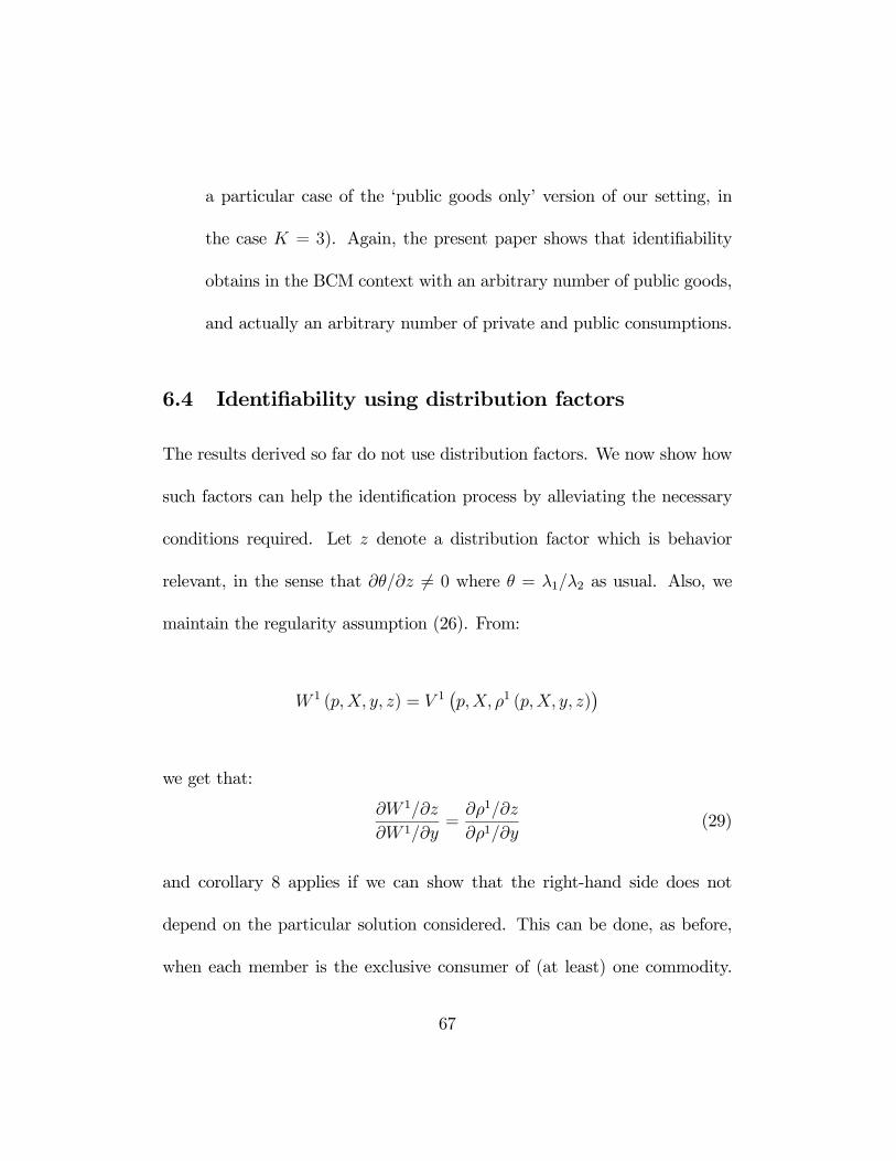
a particular case of the ‘public goods only’ version of our setting, in
the case K = 3). Again, the present paper shows that identifiability
obtains in the BCM context with an arbitrary number of public goods,
and actually an arbitrary number of private and public consumptions.
6.4 Identifiability using distribution factors
The results derived so far do not use distribution factors. We now show how
such factors can help the identification process by alleviating the necessary
conditions required. Let z denote a distribution factor which is behavior
relevant, in the sense that ∂θ/∂z 6= 0 where θ = λ1/λ2 as usual. Also, we
maintain the regularity assumption (26). From:
W 1 (p,X, y, z) = V 1¡p,X, ρ1 (p,X, y, z)
¢
we get that:
∂W 1/∂z
∂W 1/∂y=
∂ρ1/∂z
∂ρ1/∂y(29)
and corollary 8 applies if we can show that the right-hand side does not
depend on the particular solution considered. This can be done, as before,
when each member is the exclusive consumer of (at least) one commodity.
67
But this requirement can be relaxed. We only need either one exclusive good
(instead of two) or an assignable commodity. A good is assignable when
it is consumed by both members, and the consumption of each member is
independently observed.
Assume that good 1 is either assignable or exclusively consumed by mem-
ber 1, so that x11 (p,X, y, z) is observed. Now, for any two solutions, we have
that
x11 (p,X, y, z) = ξ11¡p,X, ρ1 (p,X, y, z)
¢= ξ11
¡p,X, ρ1 (p,X, y, z)
¢
where ξ11 and ξ11 denote the conditional demand of member 1 in each solution.
Therefore:
∂ρ1/∂z
∂ρ1/∂y=
∂x11/∂z
∂x11/∂y=
∂ρ1/∂z
∂ρ1/∂y
and the right-hand side of (29) does not depend on the particular solution
considered, so that identifiability obtains by corollary 8.
The genericity condition (19) may also be easier to check in that case.
Consider, in particular, the case of private goods only. Then
W 2 (p, y, z) = V 2¡p, ρ2 (p, y, z)
¢= V 2
¡p, y − ρ1 (p, y, z)
¢68
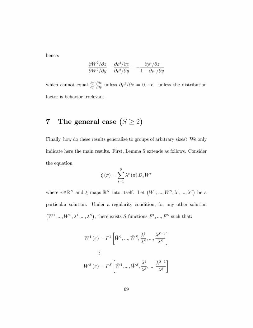
hence:
∂W 2/∂z
∂W 2/∂y=
∂ρ2/∂z
∂ρ2/∂y= − ∂ρ1/∂z
1− ∂ρ1/∂y
which cannot equal ∂ρ1/∂z∂ρ1/∂y
unless ∂ρ1/∂z = 0, i.e. unless the distribution
factor is behavior irrelevant.
7 The general case (S ≥ 2)
Finally, how do these results generalize to groups of arbitrary sizes? We only
indicate here the main results. First, Lemma 5 extends as follows. Consider
the equation
ξ (π) =SXs=1
λs (π)DπWs
where π∈RN and ξ maps RN into itself. Let¡W 1, ..., WS, λ1, ..., λS
¢be a
particular solution. Under a regularity condition, for any other solution¡W 1, ...,W S,λ1, ...,λS
¢, there exists S functions F 1, ..., FS such that:
W 1 (π) = F 1·W 1, ..., W S,
λ1
λS, ...,
λS−1
λS
¸...
WS (π) = F S·W 1, ..., WS,
λ1
λS, ...,
λS−1
λS
¸
69
where the F s satisfy moreover a set of partial differential equations. Secondly,
identifiability under exclusivity still holds in the following sense. Assume that
there exists some variable, say π1, such that ∂W 1
∂π1= 0. Then generically W 1
is identifiable. The generalized separability property extends in a similar
manner. However, both results require at least 2S commodities to apply.
Regarding economic implications, we conclude that while the general
model (without exclusivity) is clearly not identifiable, one exclusive good
per agent is sufficient to obtain generic identification in the general case,
with the same caveats as above. The techniques are similar to (although
more tedious than) those used above.
Perhaps more important is the conclusion in the presence of one distri-
bution factor (at least). Indeed, the argument previously described for two
agents directly extends to S ≥ 2. For any two solutionsW s and W s, we have
that
∂W s/∂z
∂W s/∂y=
∂x1s/∂z
∂x1s/∂y=
∂W s/∂z
∂W s/∂y
Provided that the genericity conditions are satisfied (in particular, the ∂ρs/∂z∂ρs/∂y
must be pairwise different), we then conclude that the W s are (ordinally)
exactly identified, without restriction on the number of distribution factors.
70

8 Conclusion
The main goal of the paper is to assess under which conditions the aggregate
behavior of a group provides enough information to recover the underlying
structure (i.e., preferences and the decision process) even when nothing is
known (or observed) about the intra household decision making mechanism
beyond efficiency. We reach two main conclusions. First, the general version
of the model is not identifiable: a continuum of different models generate the
same household demand function. Secondly, the existence of an exclusive
good for each member is sufficient to generically guarantee full identifiability
of the collective indirect utility of each member, i.e. of the welfare-relevant
concept that summarize preferences and the decision processes.
We adopt throughout the paper a ’non parametric’ standpoint, in the
sense that our results do not rely on specific functional form assumptions.
Obviously, the introduction of a particular functional form is likely to con-
siderably facilitate identifiability; that is, it may well be the case that, for
models that are not identifiable in the non parametric sense, all parameters
of a given functional form can be exactly identifiable, even when the form is
quite flexible. In the end, the results above show that not much is needed
to formulate normative judgements that take into account the complex na-
71

ture of collective decision processes; one exclusive commodity per agent is
’generically’ sufficient.
Constant Pareto weights Our identification is only ‘generic’, in the sense
that one can always construct examples in which it does not hold. A polar
case in which identifiability does not obtain is when Pareto weights are con-
stant; then we are in a ‘unitary’ context, since the group behaves as a single
consumer. We conclude that non-unitary models are necessary for identifia-
bility.
It is fair to argue, however, that in basically any ‘reasonable’, non unitary
model that generates Pareto efficient allocations, Pareto weights will not be
constant. Take, for instance, a simple bargaining framework, as used (among
many others) by Mc Elroy (1990) or Chiappori and Donni (2005). A key role
in determining the outcome on the Pareto frontier is played by agents’ ‘threat
points’. Various versions have been proposed for these: utilities in case of
divorce, non cooperative outcomes, ’separate sphere’ allocations, etc. In all
cases, however, the threat point is an indirect utility, representing what the
welfare an agent would achieve in some particular context; as such, they are
price dependent.
72

The exclusivity assumption These ideas have actually been empirically
implemented in a number of existing contributions. Most of the time, the
exclusive good is taken to be leisure, as in Fortin and Lacroix (1997), Blun-
dell et al. (2000), Dauphin and Fortin (2001), Vermeulen (2001), Chiappori,
Fortin and Lacroix (2002), Dauphin (2003), Mazzocco (2003a,b) and Donni
(2004). Exclusivity of leisure is certainly a strong assumption, for two rea-
sons. First, household members may spend time on household production;
note, however, that household production can readily be taken into account
in this context, as discussed in Subsection 7.2 and in Apps and Rees (1996,
1997), Chiappori (1988b) and Rapoport et al. (2003). Secondly, leisure may
be partly public, in the sense that the husband may derive direct utility from
his wife’s leisure and conversely. Therefore, if leisure is ‘mainly’ private (in
the sense that the externalities just mentioned are of second order), the ap-
proach adopted in the literature is valid. If, on the contrary, public effects
are paramount and drive most couples’ behavior, the strategy under consid-
eration may be problematic. In the end, whether leisure may be considered
as exclusive is an empirical issue. It is therefore interesting to note that
(i) almost none of the empirical tests of the collective model with exclusive
labor supply reject the specific predictions generated by the exclusivity as-
73

sumption, and (ii) in particular, papers aimed at comparing the respective
empirical performances of the unitary and the collective approach with ex-
clusive household labor supply invariably favor the latter (Fortin and Lacroix
1997, Vermeulen 2001).
Anyhow, the results derived in the present paper show that the exclu-
sivity assumption can be relaxed in two directions. First, in the presence
of distribution factors, one leisure only needs to be exclusive. This finding
should lead to new empirical approaches. Secondly, even if both individual
labor supplies are public, the model remains identifiable provided that two
alternative, exclusive commodities (one only with a distribution factor) can
be found. See Fong and Zhang (2001) for a careful analysis along these lines.
An alternative strategy considers specific consumption goods as exclusive.
For instance, several papers, following an early contribution by Browning et
al. (1984), use clothing expenditures. While assignability of clothing is not
too problematic (except maybe for same sex couples), exclusivity may be
trickier in our context, since it requires different prices for the various exclu-
sive goods. In practice, while different prices for male and female clothing
may be available, they tend to be highly correlated. Here, the result, demon-
strated in the present paper, that assignability is sufficient for identifiability
74

in the presence of a distribution factor provides a strong justification to these
approaches.
Identification Finally, what about actual identification of an identifiable
model? Specifically, what type of stochastic structure should be used, and
to what data can it be applied?
Data set are readily available (and have been used) for models of house-
hold labor supply (see the abundant literature referred to above). The case
of consumption goods is somewhat different. A standard problem of de-
mand analysis is that while income effects are usually easy to estimate, the
measurement of price effects require price variations, which may be hard
to obtain. Two strategies have been used in the literature. One relies on
variations through time and regions (see for instance Browning and Chiap-
pori 1998 and Browning, Chiappori and Lewbel 2005). Alternatively, one
may use natural experiments to generate exogenous price variations. For
instance, Kapan (2006) uses Turkish data collected in a period of high infla-
tion; similar households then face widely different relative prices depending
on the month during which they are surveyed. Both works reject the unitary
model when applied to couples, but not for singles; moreover, none rejects
75

the collective model for couples.
Regarding the stochastic structure, on the other hand, existing works use
mostly the standard approach of consumer theory, in which stochastic er-
ror terms (reflecting measurement errors, but also unobserved heterogeneity,
etc.) enter demand equations additively. Identification is in general easy to
achieve in this context. Some models, however consider more sophisticated
stochastic structure, and discuss the related identification issues; see Blundell
et al (2000) in the case of labor supply.
All in all, it is fair to conclude that much still has to be done in terms of
empirical applications of the collective model. The main goal of the present
paper is to provide a theoretical background for such works. One thing
seems however clear: whenever issues related to intrahousehold allocation
of commodities, welfare or decision power are at stake, non unitary models
are needed. The collective approach provides a consistent and promising
theoretical framework for that purpose.
76
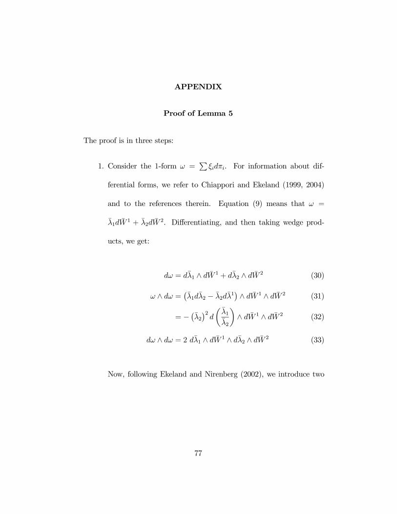
APPENDIX
Proof of Lemma 5
The proof is in three steps:
1. Consider the 1-form ω =P
ξidπi. For information about dif-
ferential forms, we refer to Chiappori and Ekeland (1999, 2004)
and to the references therein. Equation (9) means that ω =
λ1dW1 + λ2dW
2. Differentiating, and then taking wedge prod-
ucts, we get:
dω = dλ1 ∧ dW 1 + dλ2 ∧ dW 2 (30)
ω ∧ dω = ¡λ1dλ2 − λ2dλ1¢ ∧ dW 1 ∧ dW 2 (31)
= − ¡λ2¢2 dµ λ1λ2
¶∧ dW 1 ∧ dW 2 (32)
dω ∧ dω = 2 dλ1 ∧ dW 1 ∧ dλ2 ∧ dW 2 (33)
Now, following Ekeland and Nirenberg (2002), we introduce two
77
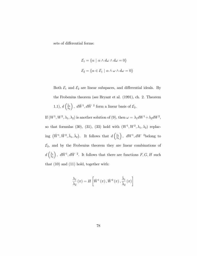
sets of differential forms:
E1 = α | α ∧ dω ∧ dω = 0
E2 = α ∈ E1 | α ∧ ω ∧ dω = 0
Both E1 and E2 are linear subspaces, and differential ideals. By
the Frobenius theorem (see Bryant et al. (1991), ch. 2. Theorem
1.1), d³λ1λ2
´, dW 1, dW 2 form a linear basis of E2.
If (W 1,W 2,λ1,λ2) is another solution of (9), then ω = λ1dW1+λ2dW
2,
so that formulas (30), (31), (33) hold with (W 1,W 2,λ1,λ2) replac-
ing¡W 1, W 2, λ1, λ2
¢. It follows that d
³λ1λ2
´, dW 1, dW 2belong to
E2, and by the Frobenius theorem they are linear combinations of
d³λ1λ2
´, dW 1, dW 2. It follows that there are functions F,G,H such
that (10) and (11) hold, together with:
λ1λ2(π) = H
·W 1 (π) , W 2 (π) ,
λ1λ2(π)
¸
78
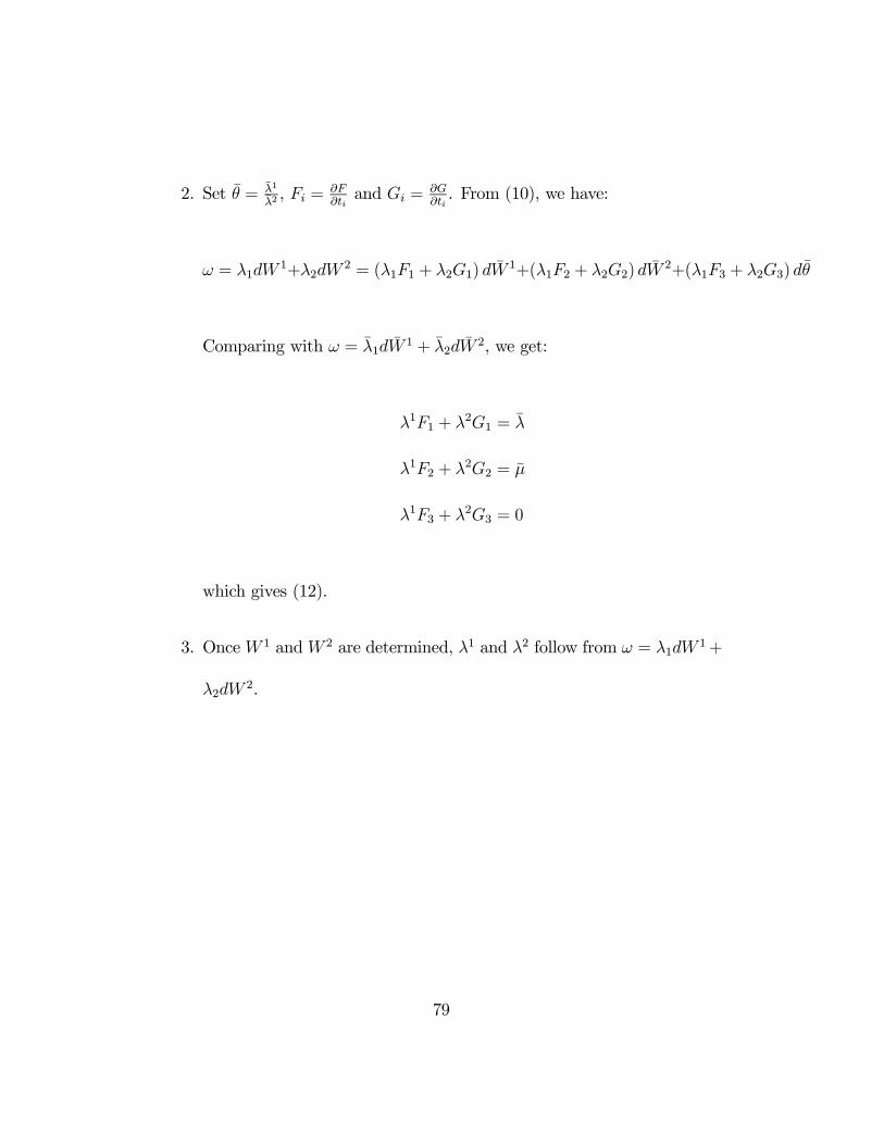
2. Set θ = λ1
λ2, Fi = ∂F
∂tiand Gi = ∂G
∂ti. From (10), we have:
ω = λ1dW1+λ2dW
2 = (λ1F1 + λ2G1) dW1+(λ1F2 + λ2G2) dW
2+(λ1F3 + λ2G3) dθ
Comparing with ω = λ1dW1 + λ2dW
2, we get:
λ1F1 + λ2G1 = λ
λ1F2 + λ2G2 = µ
λ1F3 + λ2G3 = 0
which gives (12).
3. OnceW 1 andW 2 are determined, λ1 and λ2 follow from ω = λ1dW1+
λ2dW2.
79
References
References
[1] Apps P.F. et R. Rees, 1996, ‘Labour supply, household production andintra-family welfare distribution’. Journal of Public Economics, vol. 60,pp. 199—219.
[2] Apps P.F. et R. Rees,1997, ‘Collective labour supply and household pro-duction’. Journal of Political Economy, vol. 105, pp. 178—190.
[3] Arnold, V.I. : ”Mathematical Methods of Classical Mechanics”, Springer-Verlag, 1978
[4] Bertrand, M. S. Mullainathan and D. Miller (2001), ”Public Policy andExtended Families: Evidence from South Africa”, mimeo, MIT.
[5] Blundell, R., P.A. Chiappori and C. Meghir (2005), ”Collective LaborSupply With Children”, Journal of Political Economy, forthcoming.
[6] Blundell, R., P.A. Chiappori, T. Magnac and C. Meghir (2000), ”Collec-tive Labor Supply: Heterogeneity and Nonparticipation”, Mimeo, UCL.
[7] Bourguignon, F., M. Browning and P.-A. Chiappori (1995), “The Col-lective Approach to Household Behaviour”,Working Paper 95-04, Paris:DELTA.
[8] Browning, M., F. Bourguignon, P.-A. Chiappori and V. Lechene (1994),“Incomes and Outcomes: A Structural Model of Intra—Household Allo-cation”, Journal of Political Economy, 102, 1067—1096.
[9] Browning, M. and P.-A. Chiappori (1998), ”Efficient intra-household al-locations: A general characterization and empirical tests”, Econometrica66, 1241-1278.
[10] Browning, M., P.-A. Chiappori and A. Lewbel (2005), ”Estimating Con-sumption Economies of Scale, Adult Equivalence Scales, and HouseholdBargaining Power”, Mimeo, Boston College.
80
[11] Bryant, R.L., S.S. Chern, R.B. Gardner, H.L. Goldschmidt and P.A.Griffiths : ”Exterior Differential Systems”, Springer-Verlag, New York,1991
[12] Cartan, E. : ”Les systèmes différentiels extérieurs et leurs applicationsgéométriques”, Hermann, Paris, 1945
[13] Chiappori, P.-A. (1988a), ‘Rational Household Labor Supply’, Econo-metrica, 56, 63-89.
[14] Chiappori P.A., 1988b, ‘Nash-bargained household decisions: a com-ment’. International Economic Review, vol. 29, pp. 791—796.
[15] Chiappori, P.-A. (1992), ‘Collective Labor Supply and Welfare’, Journalof Political Economy, 100, 437-67.
[16] Chiappori, P.-A. (1997), ”Introducing Household Production in Collec-tive Models of Labor Supply”, Journal of Political Economy, 105, 191-209
[17] Chiappori, P.A., R., Blundell and C., Meghir (2001), ”Collective LaborSupply with Children”, mimeo.
[18] Chiappori, P.A., and I. Ekeland (1997): ”A Convex Darboux Theorem”,Annali della Scuola Normale Superiore di Pisa, 4.25, 287-97
[19] Chiappori, P.A., and I. Ekeland (1999): ”Aggregation and Market De-mand : an Exterior Differential Calculus Viewpoint”, Econometrica, 676, 1435-58
[20] Chiappori, P.-A. and I. Ekeland (2006), ”The Microeconomics of GroupBehavior: General Characterization”, Journal of Economic Theory, 130(1) 1-26
[21] Chiappori, P.-A., Fortin, B. and G. Lacroix (2002), “Marriage Market,Divorce Legislation and Household Labor Supply”, Journal of PoliticalEconomy, 110 1, 37-72
[22] Chiappori, P. A. and B. Salanié (2000), ’Empirical Applications of Con-tract Theory: a survey of some recent work’, invited lecture, WorldCongress of the Econometric Society; forthcoming in Advances in Eco-nomics, M. Dewatripont and L. Hansen, ed.
81
[23] Dauphin A., 2003, ‘Rationalité collective des ménages comportantplusieurs membres: résultats théoriques et applications au Burkina Faso’.Thèse de doctorat, Université Laval.
[24] Dauphin A. et B. Fortin, 2001, ‘A test of collective rationality for multi-person households’. Economic Letters, vol. 71, pp. 211—216.
[25] Donni O., 2003, ‘Collective household labor supply: non-participationand income taxation’. Journal of Public Economics, vol. 87, pp. 1179—1198.
[26] Donni O., 2004, ‘A collective model of household behavior with privateand public goods: theory and some evidence from U.S. data’. WorkingPaper, CIRPEE.
[27] Duflo (2000),“Grandmothers and Granddaughters: Old Age Pensionand Intra-household Allocation in South Africa”, World Bank EconomicReview, vol. 17, no. 1, 2003, pp. 1-25
[28] Ekeland, I., and L. Nirenberg (2002): ”The Convex Darboux Theorem”,to appear, Methods and Applications of Analysis, 9, 329-344
[29] Fong, Y and J. Zhang (2001), ‘The Identifiability of Unobservable In-dependent and Spousal Leisure’, Journal of Political Economy, 109(1),191-202.
[30] Fortin, Bernard and Lacroix, Guy (1997), A Test of Neoclassical andCollective Models of Household Labor Supply, Economic Journal, 107,933-955.
[31] Galasso, E. (1999): ”Intrahousehold Allocation and Child Labor in In-donesia”, Mimeo, BC.
[32] Koopmans, T. (1949): ”Identifiability Problems in Economic ModelConstruction”, Econometrica, 17 2, 125-44.
[33] Laisney F. (éditeur), 2004, ‘Welfare analysis of fiscal and social securityreforms in Europe: does the representation of family decision processmatter?’, Review of Economics of the Household (à paraître).
82
[34] Mazzocco, M., (2003a), ”Household Intertemporal Behavior: a Collec-tive Characterization and a Test of Commitment,” Manuscript, Depart-ment of Economics, University of Wisconsin.
[35] Mazzocco M., 2003b, ‘Individual Euler equations rather than householdEuler equations’. Manuscrit, University of Wisconsin-Madison.
[36] McElroy, Marjorie B. (1990), ”The Empirical Content of Nash BargainedHousehold Behavior”, Journal of Human Resources, 25(4), 559-83.
[37] Oreffice, S. (2005), ”Did The Legalization of Abortion Increase Women’sHousehold Bargaining Power? Evidence from Labor Supply”, Mimeo,Clemso University.
[38] Rapoport, B., Sofer, C. et Solaz, A. (2003) “ Household Production in aCollective Model: Some New Results” Cahiers de la MSE, série blanche,n 03039,
[39] Rubalcava, L., and D. Thomas (2000), “Family Bargaining and Wel-fare”, Mimeo RAND, UCLA.
[40] Thomas, D. (1990), “Intra—Household Resource Allocation: An Inferen-tial Approach”, Journal of Human Resources, 25, 635—664.
[41] Thomas, D., Contreras, D. and E. Frankenberg (1997). ”Child Healthand the Distribution of Household Resources at Marriage.” MimeoRAND, UCLA.
[42] Townsend, R. (1994), “Risk and Insurance in Village India”, Economet-rica, 62, 539-591.
[43] Vermeulen F., 2005, "And the winner is... An empirical evaluation oftwo competing approaches to household labour supply", Empirical Eco-nomics, 30 (3), 711-34
83
Recommended