1

The Implications of Capital Investments for Future Profitability and Stock Returns—an Overinvestment Perspective

Donglin Li*

Haas School of Business, University of California, Berkeley, CA94720

Phone: (510) 549 2318 Email: dli@haas.berkeley.edu

January 2004

Abstract

This paper examines whether overinvestment can partially explain the negative association between capital investments (long term asset accruals), future profitability and stock returns. Capital investment has a robust negative implication for future profitability. The negative association is stronger when firms have greater investment discretion, i.e., for those firms with higher free cash flow and lower leverage. Moreover, the negative association between investment, future profitability and stock returns is almost exclusively driven by positive discretionary investment, i.e., where overinvestment is more likely to occur, rather than by negative discretionary investment, where overinvestment is much less likely. Evidence in this study provides an underlying explanation for Titman, Wei and Xie (2003)’s notion that managers’ empire building behavior is responsible for the negative association between capital investment and future stock returns. In addition, to the extent that long term asset accruals capture investment intensity, the results here may also provide an alternative interpretation of the long term asset accrual anomaly.

Keywords: Overinvestment, Free Cash Flow, Market Efficiency, Financial Statement Analysis. _______________ * I am most indebted to Terry Marsh, for his invaluable guidance and advice. I would also like to thank Bok Baik, Sunil Dutta, Qingtao Fan, Tatiana Fedyak, George Li, Maria Nondorf, Mark Seasholes, Wenbin Wei, Xiao-Jun Zhang and other participants of Berkeley accounting workshop. All remaining errors are mine. Special thanks to Scott Richardson for the codes on Mishkin tests.

2

1. Introduction

Capital investments represent a fundamental signal claimed by analysts to be useful in predicting

future profitability and stock returns (Lev and Thiagrajan (1993)). It is also of central importance in

corporate finance research whether firms make sub-optimal investments, and whether market

participants fully understand the implications of managers’ incentives to deviate from optimal

investment levels when they have the latitude to do so. This paper examines whether the overinvestment

can partially explain the negative associations between capital investments, future profitability and

stock returns.

Given the huge amount of capital expenditure by Corporate America each year (e.g, in 2001 the

total capital expenditure reaches 1.3 trillion dollars), it is surprising that so few studies have addressed

the implications of capital investments for future profitability. In the financial statement analysis

literature, Fairfield, Whisenant and Yohn (2003a) document a negative association between growth in

net long term operating assets and one year ahead future return on assets. Richardson, Sloan, Soliman

and Tuna (2003) find a similar association and attribute it to the lower reliability of long term asset

accruals. It is reasonable, though, to believe that growth in long term asset accruals also capture

investment intensity1. Abarbanell and Bushee (1997) show that capital expenditure conveys a negative

signal for future earnings. Thus, there seems to be a negative relation between capital investment and

future profitability. However, there is little evidence as to what factors could explain this negative

association. I study this association from an overinvestment perspective, along with the degree to which

the negative association between investment and future profitability is consistent with the negative

association between investment and future stock returns.

Titman, Wei and Xie (2003a) report that the negative association between capital investments and

future stock returns is stronger in firms with higher free cash flow and lower leverage. They interpret

their evidence as investor under-reaction to the overinvestment behavior by managers with empire

building incentives. However, it is not clear whether it is omitted risk factors or value destroying

discretionary investments that drive their results2. To further unravel the underlying causes, I

investigate how free cash flow and leverage can affect the association between capital investment and

future operating performance. A significant finding would provide an underlying link to support Titman

1 In appendix B, I show these variables are highly correlated with investment opportunities and future realized firm growth. Richardson, Sloan, Soliman and Tuna (2003) also call change in non-current operating assets as “investing” accruals. 2 Some researchers suggest that investment growth may be a factor in asset pricing (Berk, Green and Naik (1999), and Li, Vassalou, and Xing (2001)).

3

et al’s results and strengthen the overinvestment explanation3.

There are a lot of anecdotes suggesting that managers prefer to expand their companies faster than

they should. For example, prior to its leveraged buyout (LBO) in 1988, RJR Nabisco’s baking unit

devised a plan to revamp and modernize its baking facility at a cost of $2.8 billion. The annual savings

from the modernization would have been only $148 million, providing a pretax return of only 5 percent.

After the LBO, the modernization plan was scaled back4. More generally, the idea that overinvestment

might potentially explain the negative association between investments and future profitability is not

totally new, e.g., Abarbanell and Bushee (1997) conjectured that capital expenditures could be a bad

signal for future earnings if poor performing firms take on excessive projects, though they did not

specifically investigate this issue.

If overinvestment can partially explain the negative association between investment and future

profitability, we would also expect to observe a stronger result in the sample where overinvestment is

more likely to occur. I argue that overinvestment is more likely to occur in the sample where firms make

positive investment than firms that divest, where there may be even under investment. This assumes that

all firms have neutral investment opportunities. To better control investment opportunities, I also

constructs a parsimonious model of discretionary investment—defined as investment not warranted by

investment opportunities—and examines whether the negative associations are stronger in the positive

discretionary investment sample than in the negative discretionary investment sample. Since

overinvestment is more likely present in the former group, I expect to see a stronger association in that

group. Note that other explanations such as a growth effect by Fairfield et al (2003a) or accrual

reliability effect by Richardson et al (2003) make no such predictions. Thus, results would provide

further evidence differentiating the overinvestment explanation from others.

Consistent with my hypotheses, the negative association between investment and future

profitability is stronger in firms with high free cash flow and lower leverages. Applying a parsimonious

model to decompose investment into a non-discretionary portion and a discretionary portion, I find that

the negative association is mostly explained by the positive (discretionary) investment sample.

Next, I examine whether the market can fully incorporate the implications of capital investments for

future profitability. There is a significant negative association between firm investment and future stock

returns and the association is mostly driven by the positive “discretionary” investment sample. An

3 Studying the implication of capital investment for future profitability is also consistent with the view expressed by Penman (1992) that predicting operating performance, as opposed to explaining security returns, should be the central task of financial statement analysis. 4 The Wall Street Journal, Mar. 14, 1989.

4

investment strategy which goes long in the lowest decile of investment and short in the highest decile of

investment appears to generate persistent hedge returns. The abnormal return remains significant after

controlling firm characteristics and risk factors commonly known to be associated with stock returns.

This study contributes to the extant literatures of agency theory in corporate finance, financial

statement analysis, market efficiency, and investment measurement. First and foremost, it provides

evidence about how agency costs (proxied by free cash flow and leverage) affect the association

between investments and future operating performance: the negative implications of high capital

investments are stronger for firms with high free cash flow and lower leverages. This reinforces

Jensen’s and Titman et al’s notion that empire building incentives drive the negative association

between capital investment and future stock returns. My results are also consistent with recent findings

in Hennessy and Levy (2002) that empire building incentives appear to be the dominant agency issue

distorting firm investment. Second, I empirically validate several commonly used measures of

investment and find that long term asset accruals are good proxies of investment intensity. To the extent

that long term asset accruals capture capital investment intensity, if agency costs can explain the

negative association between investments and future profitability, they could potentially explain the

negative association between long term asset accruals and future profitability. This paper thus provides

a new perspective on the long term asset accruals anomaly that is distinct and perhaps not mutually

exclusive from the reliability conjecture by Richardson et al and growth explanation by Fairfield et al.

Third, I document a strong stock market return anomaly associated with firm investments. The finding

casts doubt on the efficient market hypothesis. The negative association between investments and

future returns is robust to various risk factors and other potentially associated anomalies. The results

may be of interest to financial statement users, such as managers, analysts and creditors who are

interested in understanding the implications of capital investment for firm performance. Last, I validate

several commonly used measures of investment which should benefit future studies.

The remainder of the paper is organized as follows. In section 2, I briefly describe prior research on

investment and stock returns and develop hypotheses. Section 3 discusses the sample and variable

measurements while section 4 presents empirical tests. Section 5 provides concluding remarks.

Appendix A describes variable definitions while Appendix B validates investments proxies.

5

2. Literature and Hypotheses Development

2.1 Literature

The corporate finance literature is not settled as to whether firms in general tend to over invest or

under invest5. Empirically there is mixed evidence as to how the market responds to capital

investments6. Beneish, Lee and Tarpley (2001) find that the magnitude of capital expenditures is

negatively related to future stock performance. Abarbanell and Bushee (1998) report that

industry-adjusted capital expenditure growth is negatively associated with future returns, a result

contradictory to their hypothesis. Titman et al (2003a) find a similar negative relation and provide

evidence that firm over-investment is responsible for this negative association. Titman et al (2003 b)

compare Japanese keiretsu firms and independent firms and find that in the former groups there is a

negative association between investment and future returns while in the latter the association is positive.

The result is consistent with the idea that keiretsu firms, which have low-cost access to capital, tend to

over invest. Hennessy and Levy (2002) find that empire building is the dominant factor leading firms to

over invest. None of these studies examines the implication of investments for future profitability.

The fundamental analysis literature has documented that various accounting items are predictive of

future earnings (e.g., Penman and Zhang (2002)). Abarbanell and Bushee (1997) examine the

implication of several fundamental signals, including a measure of industry-adjusted growth in capital

expenditures, for future profitability. However, their sample size is much smaller than mine (because of

the requirement of earnings forecast data) and their use of earnings per share as the dependant variable

is subject to critic issue that scale effects influence the results (Easton (1998)).

It is important that research contributes not only to identifying variables that can predict future

profitability, but also to providing economic interpretation of the variables. Current explanations are

mostly conjectures with no supporting evidence. Fairfield, Whisenant and Yohn (2003a) find that two

components of the annual changes in net operating assets--- accruals and long term operating

accruals---are equally strong negative predictors of one-year accounting return on total assets and of

5 In fact, a finding that investment is more sensitive to cash flows is subject to different interpretations: capital rationing and hence under investment (Fazzari et al 1988), over investment (Kaplan and Zingales (1997), Jensen (1986)). Without examining the implication of such investment for future profitability, it is difficult to distinguish the two contradicting theories. 6 In event studies, McConnell and Muscarella (1985) indicate that announcements of increase in planned capital investments are generally associated with significantly positive excess stock returns. Blose and Shieh (1997) and Vogot (1997) find that market reacts to the level of capital investment announcement. Another set of studies examines the valuation effects of actual capital investment using annual returns and the results are mixed. Even studies may be subject to two problems, though. First, firms may self select to announce investment plans. Second, market may misprice the investment in a short window, which is a valid concern. In fact, in the longer window I studies, market seems cannot fully understand the implication of investment on future earnings. Lev and Thiagarajan (1993) find out that industry adjusted capital expenditure growth is positively associated with contemporary returns, while Abarbanell and Bushee (1997) find no such association. Park and Pincus (2003) find incremental information content of capital expenditures beyond unexpected earnings.

6

stock returns. They conjecture that the accrual anomaly documented by Sloan (1996) is actually a

growth effect caused by diminished returns from investment or conservative accounting. However,

Fairfield et al only examined the implication of growth in net operating assets for one-year-ahead

profitability. While discussing Fairfield, Whisenant and Yohn (2003b), Dichev (2003) argues that the

relation between growth and future profitability has more of a time-series flavor that has not been

documented: this study could be interpreted as filling the impact of capital investment on one to twenty

years ahead performance.

Richardson, Sloan, Soliman and Tuna (2003) find that investors misinterpret the information

contained in various operating and financing accrual items. They argue that different reliabilities

associated with various operating accruals, either current or non-current, should result in different

implications for future earnings and stock returns. While highly convincing, their study furnishes little

evidence on why some accruals are more or less reliable than others. Richardson and Sloan (2003)

construct three measures of net external financing and find that there is a systematic strong and negative

relation between external financing and future stock returns. Based on the finding that future stock

returns are negatively related to changes in operating assets, they suggest that a potential explanation is

firm over-investment in operating assets. However, in the same paper, they also try to add an accrual

manipulation explanation.

There is much empirical evidence that suggests that free cash flow can exacerbate firm

overinvestment (e.g., Kaplan (1989), Blanchard et al (1994)) while debt can mitigate overinvestment

(e.g., Harvey, Lins and Roper (2001)). Results in this study are consistent with above findings.

2.2 Hypotheses Development

I first confirm that high investment intensity leads to decreased future profitability. Although this is

not the focus of this paper, establishing such a relation is necessary for hypotheses to follow. Despite

previous findings that document such an association, Dichev (2003) argues that capital investments

could be positively related to future profitability, e.g., if “capital follows profitability”. Given the result

that investment and future profitability are negatively related, it may be that the relation is explained by

conservative accounting. Penman (2001, 561) argues that conservative accounting could make the

profitability of new investment appear relatively less profitable in earlier years and more profitable in

later years. If conservative accounting is the only underlying force then temporarily dampened return on

assets will reverse sometime in the future years. Penman and Zhang (2002) argue that the profitability

reversal should be more likely to be observed when firm investment growth slows down in the future. If

this is true then capital investment may be a positive portent for long term future profitability. This leads

7

to my first hypothesis, stated as an alternative to reverse:

H1: The negative association between investment and future profitability will not reverse in longer

periods.

If the results are consistent with hypothesis H1, we can infer that there is an economic explanation

for the investment-future profitability association.

While even optimal investment may lead to lower profitability ratios caused by diminished

marginal rate of return, suboptimal investment can further impact profitability. The separation of

management and ownership creates the potential for management to engage in suboptimal activities

including empire building behavior. Managers of firms with high free cash flow can act

opportunistically and indulge in ‘value destroying activities’ and to ‘over invest and misuse the funds’

(Jensen (1986)). Excessive free cash flow enables managers to invest in negative NPV projects after

exhausting positive NPV projects (Blanchard et al (1994), Richardson (2002)). On the other hand, when

firms have a cash short fall, the possibility of over investment is mitigated because the firm is forced to

raise funds through external markets, which provide a monitoring role. If wanton overinvestment results

in lower future profitability, ceteris paribus, we would expect to observe a more negative relation

between capital investment and future profitability for high free cash flow firms. On the other hand,

capital rationing theory7 (Myers and Majluf (1984), Fazzari et al (1988)) predict that high free cash flow

and high cash holdings can benefit a firm by reducing the cost of information asymmetry that places a

wedge between the costs of internal and external capital. Thus high free cash flow enable firms to make

optimal investment with less cost and obtain better future operating performance. I expect the

overinvestment effect dominate the cash rationing effect.

Leverage could potentially mitigate the overinvestment problem. Leverage restricts the use of

internal funds generated by the firm by forcing managers to use cash flow to meet contractual financial

obligations (Jensen (1986), Stulz (1990)). Managers’ empire building incentives may be constrained by

creditors’ legal rights to reorganize or even liquidate the firm in case of default. The debt market also

provides management discipline (Rubin (1990)). Thus, the negative association between investment

and future profitability could reasonably be expected to be weaker in firms with high leverage.

However, debt cannot perfectly solve the problem (Grinblatt and Titman (1998)). Lyandres and

Zhdanov (2003) also emphasized that capital structure cannot by itself induce managers to invest

optimally. High leverage also brings agency cost, e.g., bankruptcy cost. Thus, I expect the effect from

7 Recently there is increasing evidence questioning capital rationing theory (Kaplan and Zingales (1997), Cleary (1999) and Alti (2003)).

8

leverage is of second order and weaker than that from free cash flow. This leads to my main hypothesis,

stated in alternative form:

H2a: The negative association between investment and future profitability will be stronger in firms

with higher free cash flow, ceteris paribus.

H2b: The negative association between investment and future profitability will be weaker in firms

with higher leverage, ceteris paribus.

If overinvestment can partially explain the negative association between investment and future

profitability, we would also expect to observe a stronger result in a sample where overinvestment is

more likely to occur. The negative association probably would disappear in a sample of firm

underinvestment, where the association may be even positive. I argue that overinvestment is more likely

to occur in the sample where firms make positive investment than firms that divest8. This holds if all

firms have equally neutral investment opportunities. To better control investment opportunities, I also

construct a parsimonious model of discretionary investment (defined as investment not warranted by

investment opportunities, for estimation see section 3.2 and appendix B) and examine whether the

negative associations are stronger in the positive discretionary investment sample than in the negative

discretionary investment sample. Since overinvestment is more likely present in the former group,

where the detriment in firm value will manifest in lower future profitability, I expect to see a stronger

negative association in that group.

If negative discretionary investment correctly captures underinvestment, there should be weaker or

even positive association in the negative discretionary investment group. However, if firms generally

over invest, as documented in Hennessy and Levy (2002) and Richardson (2002), then my model that

tries to statistically parse out discretionary and non-discretionary investment may result in some

estimation error, i.e., positive discretionary investment is more likely over investment, but negative

discretionary investment could be either underinvestment, over investment or simply estimation error.

Thus, there is no clear prediction on the sign of the association between investment and future

profitability in the negative discretionary investment group. Thus, I expect:

H3: The negative association between investment and future profitability is stronger in the sample of

positive (discretionary ) investment firms than in the sample of negative(discretionary) investment

firms.

8 Beyond free cash flow and leverages, there may be other agency costs or asymmetric information that affect firms to make suboptimal investment (e.g., Myers and Majluf (1984), Dechow and Sloan (1991)). Although some researchers argue that overinvestment is the dominant effect (Hennessy and Levy (2002) and Richardson (2002)), others provide evidence of underinvestment (Aggarwal et al (1999)).

9

Note that other theories such as accrual manipulation make no such prediction. Thus tests of H3

may to some extent distinguish the overinvestment explanation from the accrual reliability explanation

which claims that long term operating accruals are measured with error, and the growth explanation

which recognizes that when firms make investments, firms would grow in sizes.

The next hypothesis is based on the growing evidence that the market often does not fully

understand the implications of financial statements items (e.g., Sloan (1996), Holthausen and Larker

(1992)). If investors do not understand the negative implications of investment for future earnings, then

a strategy that exploits this information can earn abnormal returns. Titman et al (2003) argue that empire

building managers may have an incentive to put the best spin on their investment opportunities as well

as on their over all business when they make high capital investments, perhaps to justify their action. If

investors fail to recognize the over investment behavior or are fooled by the rosy picture of firm

performance, then the subsequent-period stock returns of firms that made excessive investment may

deteriorate as overinvestment results in lower than expected performance. Moreover, the price

correction might be expected to concentrate around earnings announcements. Based on hypotheses 2

and 3, I also predict the following:

H4a: The negative association between investments and future stock returns will be stronger in

firms with higher free cash flow and lower leverage.

H4b: The negative association between investments and future stock returns will be stronger in

firms of positive (discretionary) investment than in firms of negative (discretionary) investment.

3. Sample, Variable Measurement and Descriptive Statistics

3.1 Sample

Firms’ financial statement data are obtained from the Compustat annual active and research

databases and stock returns data are from the CRSP daily returns files. I use annual Compustat data

instead of quarterly data because firms’ investing activities are not uniform during a year (Callen et al

(1996)). I start my sample from 1962 because from that year the data is available for a substantial

number of firms and also because Compustat data prior to 1962 suffers from serious survivorship bias

(Sloan (1996)). Financial firms (SIC codes 6000-6999) are excluded because their investing, operating

and financing activities may be not clearly demarcated. The full sample consists of 133, 277 firm-year

observations representing 14, 446 firms from 1962 to 2002 to be included in my least restrictive test.

The number of observations in any particular test will vary depending on requirements of the test.

10

3.2 Investment Measures and Model of Discretionary Investment

In this section I show that long term asset accruals (e.g., change in net PPE or long term asset) and

capital expenditures are both strong proxies of investment intensity. My results in later tests are robust

with respect to the use of each variable. In addition, the question of what is a good measure of

investment intensity is itself of great practical value and surprisingly, no previous studies of the relative

properties of various measures seem to exist.

I begin by choosing a benchmark that relates investment with investment opportunities9. An

investment proxy that best matches investment opportunities may be considered more accurate.

Hayashi (1982) shows that under some conditions, the following equation hold10:

λα

+−+= ]1[1 QaKI (1)

where I is firm investment, K is the beginning-of-period capital stock, α is a parameter linearly

increasing in the cost of adjustment function, Q is the present value of profits from new capital

investment, and λ is some technology shock.

Based on the Hayashi model, it seems that a good measure of investment intensity should be

deflated by either PPE (property, plant and equipment) or total assets. In fact, most researchers proxy

investment with capital expenditure scaled by PPE or total assets (e.g., Kaplan and Zingales (1997),

Hennessy and Levy (2002), Minton and Chrand (1999)).

I apply the following variables to proxy investment opportunities: Tobin’s Q, profitability (ROA)

(Blanchard, Rhee and Summers (1993)), past sales growth (Shin and Stulz (1996)) and value of growth

opportunity (Vgo, Richardson (2002)).

Second, I choose a benchmark for ex post realization of investment. Investment intensity should be

reflected in future growth in sales, earnings and book value. Following an approach similar to Kallpur

and Trombley (1999) and Richardson(2002), I focus on ex post realized sales growth11 , and examine

9 Although I am only trying to evaluate whether one measure is a good proxy for investment, not necessarily optimal investment, it can be shown that under some conditions, a measure that best matches for investment opportunities is more accurate. Assume there are two measures of investment, both measuring the underlying investment intensity with errors:

1I and 2I , where

1*

1 ε++= DII and 2

*2 ε++= DII , where I* is optimal investment and D is the distorted investment resulting from information

cost or agency problem. Assuming 1ε has a smaller variance than that of 2ε and both measurement errors are independent of I, D

and Q, then it is obvious that 1I should be more closely correlated with either Q or (Q and profitability) than 2I does. Further 1I

should fit the model better than 2I in multiple variables regression.

10 Specifically, adjustment costs in investment are linearly homogeneous in investment and capital, so that marginal and average q will equal. 11 I choose not to use growth in book value or earnings as the benchmark. Growth in book value firms may bias in favor of some measures I later choose, e.g., growth in PPE.

11

how different measures of investment are correlated with it. Specifically, I estimate the correlation year

by year and significance for the mean correlation over the entire sample period is assessed by a

Newey-West (1987) t-statistics.

Now I introduce candidates of investment measures. I select several measures that are

representative of what early studies have applied:

Capital expenditure/PPE (e.g., Hennessy and Levy (2002))

(Capital expenditure-Depreciation)/total assets (e.g., Shin and Stulz (1996))

Capital expenditure/Total assets (e.g., Gompers, Ishi and Metrick (2003))

Capital expenditure/Sales (e.g., Anderson and Garcia-Feijoo (2003), Titman et al (2001))

Capital expenditure/Value (e.g., Smith and Watts (1992))

R&D/total assets (e.g. Gaver and Gaver (1993), Hall (1992))

Growth in inventory (e.g., Kashyap, Lamont and Stein (1994))

Growth in capital expenditure (e.g., Lev and Thiagarajan (1993))

Growth in number of employees (Lang, Ofek, and Stulz (1996))

I also add several measures that I contend make sense as well:

Growth in PPE12

Long term asset accruals (Change in long term asset deflated by average total assets)13

Growth in long term asset

Finally, I adopt a measure of a firm’s investment applied by Baber, Janakiraman and Kang (1996),

as the sum of capital expenditure on PPE, acquisitions, and research and development, then deflated by

depreciation expense.

Another measure INV_CS is constructed to measure the cash flows in investing activities:

-(-increase in investment + sale of investment-capital expenditure + Sale of PPE-acquisition), divided

by average total assets14.

Ex ante, we may predict the relative performance among some of these measures of investment

12 The growth measure also takes good care of possible fixed effect that may be present in other measurements. Thomas and Zhang (2002) applied a similar measure to proxy for investment: change in net PPE scaled by total assets. 13 Harrison and Horngren (2003) define investing activities as “Activities that increase or decrease the long term assets available to the business.” “(Investments) increase and decrease long-term assets, such as computers and software, land, buildings, equipment, and investments in other companies. The purchases and sales of these assets are investing activities.” (2003, P548 ). 14 The advantage of this measure is that it is most accurate in reflecting the cash spent in investing activities. A weakness of this measure is that it omits non-cash investing activities. Companies make investments that do not require cash. Non-cash investing activities can be reported in a separate schedule that accompanies the statement of cash flows. Hence, I anticipate this measure is least powerful compared to the growth in long term assets or PPE. A possibly more accurate measure can be derived from statement of cash flows (data311) and reflect how much cash is spent in investing. The disadvantage of this measure is that this measure is only available after 1987.

12

intensity. For example, capital expenditure/sales(SI ) probably would be a noisier measure than capital

expenditure/PPE (KI ) because

KS

KI

SI /= where the denominator

KS is something like a PPE

turnover ratio which varies across industries and thus introduces some noise into the ratio. Another issue

concerns capital expenditure. Note that it is almost always positive and omits retirement of any PPE.

Focusing on only capital expenditure ignores de-investment from sale of PPE and investment through

acquisition, e.g., where firms liquidate one investment item to finance another investment project. Such

transactions represent potential omitted variables and create potentially an errors-in-variables problem

in prior research. Also, using growth of capital expenditure may be problematic if there is little

expenditure in a prior year. A better measure might be simply the change in PPE divided by lagged PPE.

After all, this is what the model is supposed to relate.

To estimate discretionary and non-discretionary investment, I apply the following rank regression:

ttttt syeardummiemmiesindustrydugrowthSalesROAQINV εβββα ++++++= −−− 131211 _ (2)

These three explanatory variables, Tobin’s Q, profitability and past sales growth, have been shown

to proxy for investment opportunities. Q alone is widely known to be notoriously noisy. Alti (2003)

argues that a substantial part of Q represents the option value of long term growth potential. Since the

option value is not very informative about near term investment plans, Q does not proxy well for short

term investment opportunities. In addition, if the market is unaware of investment opportunities within a

firm, the Q measure cannot sufficiently reflect investment opportunities. Managers may also manipulate

stock prices to justify the expenditure. These issues suggest that other variables be considered as prxies

for investment opportunities. Based on the validation results in appendix A, I choose growth in PPE

(d_PPE) and long term asset accruals (INV_bs) as my measures of investments15 because of their

superior performance and because they are also measures of accruals16.

The fitted value is called to be the non-discretionary component of investment while the residual is

defined to be the discretionary investment. The explanatory power is comparable to various accrual

models with an R square of about 24%. Replacing Q with the value-of-growth-option (vgo) measure

introduced by Richardson (2002) yields almost identical results. In robustness check, I also add past

stock returns as an explanatory variable (Fama (1981)) in the model and obtain very similar results.

15 These measures in spirit are similar to the “new” investment in Richardson (2002) as they are clean of depreciation and amortization, the portion of investment seen as to maintain assets in place. 16 I choose not to combine these measures with R&D or inventory because the former has higher and the latter has lower adjustment costs than investment in PPE, while according to (1) a measure of homogeneous adjustment cost is preferred. In addition, there is little evidence that managers over invest in R&D activities, perhaps because these expenditures are expensed rather than capitalized. Moon (2001) find that the subject of overinvestment may be capital expenditure and not R&D expenditure.

13

3.3 Return Variables

This section I introduce measures of abnormal stock returns, omitting the t subscript.

Abr = Size adjusted 12month stock return, measured as the realized buy-and-hold stock returns17

from CRSP over the 12 months starting from the end of month four after the end of fiscal year t, minus

the buy-and-hold return on a value weighted portfolio of stocks having similar market capitalization.

The size portfolios are formed by CRSP and are based on size deciles of NYSE and AMEX firms. The

assignment of each stock into size portfolios is based on firm’s market capitalization at the beginning of

the fiscal year in which the return cumulating period starts.

Character = Twelve month stock returns adjusted for firm characteristics. This is another approach

I control for risk. I follow Daniel, Grinblatt, Titman and Wermers (1997) to construct excess returns

relative to benchmarks that are constructed based on firm characteristics (i.e., size, book to market ratio,

and momentum). I form 125 benchmark portfolios based on firm characteristics of size, book to market

ratio and momentum. The portfolios are formed in the following way: Starting with May of fiscal year t,

stocks are sorted into five portfolios based on each firm’s size at the end of fiscal year t-1. The

breakpoints are obtained by sorting NYSE firms into quintiles based on their size measures. The size of

stocks in my sample is then compared against the breakpoints to assign each stock into a size group.

Firms in each size portfolio are further sorted into quintiles based on the t-1 fiscal year end book to

market ratios. Last, firms in each size-bm portfolios are sorted into quintiles based on prior year’s stock

returns ending March of fiscal year t. I choose March in stead of April as the year-end to reduce the

impact of bid-ask bounce and monthly reversals. In each of the 125 portfolios, value weighted returns

are calculated monthly from May of fiscal year t to April of fiscal year t+1. Benchmark portfolios are

rebalanced each year. Each stock’s excess return, called the character-adjusted return, is then calculated

by subtracting the stock’s corresponding portfolio’s return from the stock’s return.

3.4 Free cash flow (FCF) and Leverage (L)

Jensen (1986) defines free cash flow as the portion of cash flow that remains after all positive NPV

projects are taken. However, as Lang, Stulz and Walking (1991) and Gul and Tsui (1998) pointed out,

the literature provides little guidance on the measures of FCF as defined by Jensen (1986). Researchers

often use earnings before interest, taxes and depreciation (EBITDA) or operating cash flow less interest

expense as proxies for free cash flow (e.g., Fenn and Liang 2001).Several proxies are used in the finance

17 Delisting return is applied where available. Where unavailable, I follow Shumway (1997) for NYSE/AMEX stocks and Shumway and Warther (1999) for NASDAQ stocks to correct for delisting bias. I use –0.3 as the last return for NYSE/AMEX stocks and –0.55 as the last return for NASDAQ stocks delisted for performance reasons. If the delisting code is still missing, I use –1. After the delisting and before the end of the 12th month, I assume the proceeds from delisting are reinvested in the value-weighted market

14

literature and I follow these studies to define FCF as operating income before depreciation less interest,

taxes and preferred and common dividends. Such definitions are normalized by either total assets or

total book value of equity in the previous year. I choose to scale by total assets, consistent with Lang et

al (1991), and Gul and Tsui (1998).

As robustness checks, I also apply growth in cash holdings (GrCash) as a second proxy (Harford

(1999)) and Richardson (2002)’s surplus cash measure as a third proxy.

I measure leverage as total liability divided by the sum of total liability and equity capitalization,

similar to Titman et al. I also apply debt ratio as a second proxy for leverage (Lang, Ofek, and Stulz

(1996)).

3.5 Descriptive Statistics

Table 1 provides descriptive statistics for the key variables. The median book to market ratio is

0.593 over my sample period. The median sales growth is 1.598 but the mean is 3.040, thus some firms

have undergone extreme growth. The median and mean accrual is negative, consistent with other

studies and implying cash flow from operations exceeds GAAP operating income on average. From

panel B, investment intensity (d_PPE) is positively correlated with size (log_cap) and profitability

(contemporaneous ROA); thus it seems that firms with low investment intensity are generally less

profitable and smaller in size, consistent with the notion that profitable firms tend to invest more. The

Spearman rank correlations also show that investment measures such as d_PPE , INV_bs and growth in

number of employees (d_employee) are negatively related to one year ahead size adjusted returns (Abr).

Accrual is also significantly related to future abnormal returns, confirming that the accrual anomaly is

present in my sample. Investment measures (d_PPE and INV_bs) are positively correlated with

investment opportunities (lag_q). They are also positively correlated with one year ahead ROA.

However, this correlation does not control for current ROA. Also as expected, these measures of

investment are positively correlated with past stock returns (dt), profitability (ROA) and negatively

correlated with book to market ratio, suggesting the need to control these factors in return analysis.

Except for the correlations between profitability measures in adjacent years, no correlation exceeds

50%, suggesting that multicollinearlity is unlikely to be a serious issue in subsequent regression tests.

4. Empirical Analysis

I present the empirical tests in several steps. In section 4.1 I confirm that a robust negative

association between investment and future profitability, both short term and long term. The evidence

index. Return results are not sensitive to the adjustment of delisting returns.

15

supports the notion that the association is likely to have an economic explanation. In 4.2, I examine how

free cash flow and leverage affect the relation between capital investment and future profitability. In 4.3

I break the sample into positive discretionary investment firms and negative discretionary investment

firms, and examine whether the negative association is mostly driven by the former sample where

overinvestment is more likely to occur. In 4.4 I examine whether investors fully understand the above

relations by looking at stock returns. I also examine whether the mispricing is mostly driven by positive

discretionary investment firms. Since hypothesis 4a is mostly a corroboration of Titman et al, I leave

that test in the end.

4.1 Time series relation between investment and profitability.

Test of Hypothesis 1

When firms increase investment, conservative accounting leads to reported earnings that are lower

than they would have been under liberal accounting. To test whether higher investment will depress

short term profitability but improve long term profitability, I apply the following regressions18:

ntttnt INVROAROA ++ +++= εγβα (3)

where n runs from 1 to 10 years ahead, INV stands for capital investment, ROA is operating income

scaled by average of total assets at the beginning and end of fiscal year19.

Investment will likely inflate future total assets--the denominator of ROA (Fairfield, Whisenant and

Yohn (2003b)). Thus the finding of such a negative correlation could be no more than a mechanical

relation rather than an economic one. However, this denominator effect can not last long in distant years

when capital investments are fully depreciated.

To further mitigate the possibility that the negative association is mechanical, I also examine

earnings deflated by sales (PM):

ntttnt INVPMPM ++ +++= εββα 21 (4)

Panel A of table 2 report regression results applying d_PPE as the investment measure. The

coefficient on current ROA is significant ranging from 0.707 for one year ahead ROA to 0.151 for 10

year ahead. The magnitudes of ROA persistence are similar to those reported in previous studies. The

coefficient on investment is -0.018 for one year ROA. This means that 1% growth in PPE will decrease

one year ROA by about 1.8 basis points. As n increases, the coefficients on current ROA and profit

margin (PM) get smaller, indicating stronger mean reversion of profitability over longer periods. In

addition, the negative coefficients on investment also get weaker. This suggests that the dampening

18 Industry dummies (two digit sic code) are also included in the regressions but not reported for exposition purpose.

16

effect from investment on future earnings becomes less severe in distant years. However, the

coefficients remain significantly negative out to 12 years ahead, then become insignificantly negative

thereafter. This result is inconsistent with conservative accounting which predicts that at some point the

coefficient should turn positive. Thus, conservative accounting is unlikely the only underlying cause for

the negative association20.

On the right hand side of the panel, I examine future earnings deflated by sales and obtain similar

results. In unreported results, I replace all variables by their percentile ranks and get results that are

consistent with panel A.

In panel B of table 2, I use long term asset accruals deflated by total assets (INV_bs) as a measure of

investment and obtain a similarly negative coefficient on investment for the following 10 years’

performance (ROA). The negative coefficients are bigger in magnitude than those in panel A; this might

be caused by the fact that d_PPE is positively skewed while INV_bs is more symmetrically distributed

and hence less affected by extreme values.

The relation documented above is not due to a few extreme years. For example, when regressing

one-year-ahead ROA on d_PPE, the coefficients are negative in 39 of the 40 years.21 I do not examine

tests beyond 20 years because it is not clear whether results will be reliable given the survival bias.

To further highlight the implications of capital investments for future profitability, I present

graphical evidence. I use a two-stage ranking procedure. First, I sort the sample into ten portfolios based

on ranks of current tRNOA 22. Within each decile level of tRNOA , I further sort the observations into

five portfolios based on investment intensity (d_PPE). I then pool all 10 sub-portfolios of each tRNOA

level together into one portfolio. Now I have five portfolios that have substantial variation in investment

intensity but nearly the same level of current profitability ( tRNOA ).The two way sorting ensures that

the observed relation between changes in RNOA over time and investment does not reflect the widely

19 Using operating income before depreciation does not change the results qualitatively. 20 To more directly examine whether there is profit reversal from the conservative accounting effect, I also run the following regressions:

11 +−+ +++= tnttt INVROAROA εγβα where n=2, 5, 10… If there is substantial reversal effect, we would expect to see a positive coefficient on investment. Unreported results show that most coefficients are insignificant. However, I do not assert there is no effect from conservative accounting. 21Unreported results show that other measures of investments, such as growth in number of employees, also implies decreased one year ahead ROA. Fairfield et al (2003b) raise a concern that investment is positively correlated with future total assets, the denominator of ROA. Interestingly I find out that one year ahead earnings by current year’s average total assets is also negatively affected by investments. 22 Applying RNOA rather than ROA provides a robustness check. I repeat the graphical procedure based on ROA and obtain similar patterns.

17

known profitability mean reversion. This control is important as high investment is correlated with

higher current RNOA. In figure 1, I plot the top and bottom quintiles, applying median values of

portfolio RNOA.

Figure 1 shows that, on average, RNOA is higher for high investment firms prior to year 0,

consistent with firm growth and high investment opportunities. However, after year 0, RNOA starts

deteriorating. The low investment firms report lower RNOA than the high investment firms, but by year

0 they report similar levels of RNOA as the high investment group (by construction). After year 0, high

investment firms report persistently lower profitability. In fact low investment firms continue to have

higher ROA than do high investment firms for up to 15 subsequent years. We might predict that ROA

would eventually catch up for high investment firms in later years, e.g., if the low ROA occurred

because not all the high investment expenses (benefits) are properly capitalized (recognized). However,

as shown in figure 1, the ROAs never exceed the ROAs for the low investment firms. This is

inconsistent with conservative accounting explanation which predicts that the two lines should cross

when the hidden reserve from past investment brings higher future profitability. Thus, it seems unlikely

that conservative accounting can solely explain the results23.

The above tests results are consistent with related research in Richardson et al (2003c) that assert

that Fairfield et al (2003a)’s results are not consistent with conservative accounting or diminished

returns to sale. In a related study, Abarbanell and Bushee (1997) also find evidence that the association

between capital expenditure and future earnings does not eventually reverse. Thus, a plethora of

evidence calls for an economic explanation for the association. I investigate whether overinvestment

can provide a partial explanation.

4.2 The Impact of Free cash flow and Leverage

Test of Hypothesis 2a

In panel A of table 3, I examine how the negative coefficients on investment vary with lagged free

cash flow levels, using d_PPE as the measure for investment. I sort the whole sample into five portfolios

based on levels of free cash flow levels in the year prior to investment. Then within each portfolio, I

repeat regression (3) in model 1.

In the left half of panel A, I condition the regression on FCF while on the right side I condition on

growth in cash holdings (GrCash) prior to year of investment.

To examine the effect of free cash flow beyond one year, I also conduct the following regression in

23 In fact, because of the dampening effect of increased investment, the true economic profitability of the high investment group as of year of investment may be higher than that of the lower investment group. That would further bias against not finding the

18

model 2:

522152 tttttt INVROAFROA −− +++= εββα (5)

where FROA is the average ROA from year t+2 to year t+5.

Across both the regressions for one-year-ahead ROA (model 1) and subsequent four year average

ROA (model 2), the coefficient on investment is significantly negative, except in the model 1 result for

the lowest FCF group, where it becomes marginally significant. More important, across both models the

coefficients increase monotonically (becoming more negative) as the levels of FCF rise. For example, in

model 1, the coefficient increases from -0.006 with an insignificant t statistic in the lowest FCF level

group to -0.024 with a significant t statistic in the highest FCF group. In addition, the number of years

when the coefficient is negative ranges from 29 out of 39 years in the lowest FCF group to 37 out of 39

years in the highest FCF group. Results based on GrCash are similar. Unreported rank regressions also

report similar patterns. Thus preliminary tests show that free cash flow is associated with a stronger

relationship between ment and future profitability.

Panel B of table 3 is for long term accruals (INV_bs) as a measure of investment. Again, as the free

cash flow level increases, the negative coefficient on investment increases in absolute magnitude from

-0.002 (t=-0.13) to -0.061 (t=-8.26) in model 1, and from -0.028 (t=-2.60) to -0.060 (t=-6.47) in model

2.

Test of Hypothesis 2b

Panel C of table 3 investigates the effect of leverage in the year prior to investment, using d_PPE as

the measure of investment. On the left side, I report regression results for the five portfolios ranked by

market leverage while the results on the right hand side are for rankings by debt ratio.

Clearly, leverage has an opposite effect to that of free cash flow. In model 1, the negative coefficient

decreases from -0.021to -0.007 as leverage increases. The model 2 regression for future ROA beyond

one-year-ahead exhibits a similar pattern. Using debt ratio as a robustness check yields similar

conclusions.

Panel D of table 3 uses INV_bs to proxy investment. On the left side in the table, we can see that the

coefficient decreases with leverage, although not monotonically; in the highest leverage portfolio, the

coefficient even becomes insignificant. This is consistent with the notion that leverage can mitigate the

negative association between long term asset accruals and future profitability.

Overall, results in table 3 are consistent with H2b. However, one possible concern is that the

conservative effect.

19

negative association between investment and future profitability is nonlinear. Thus the above

documented results are simply a reflection of the positive correlation between free cash flow and

investment levels and negative correlation between leverage and investment level. To address this

concern, I first sort the whole sample into 20 portfolios based on investment intensity. Then with in each

portfolio I further sort by current ROA into 20 portfolios. Within each of the 400 portfolios I rank lag

free cash flow (leverage) level into quintiles. This procedure makes sure that each free cash flow

(leverage) quintiles has similar investment and current ROA distributions. I then repeat the above tests

and obtain similar findings. Figure 2 plots regression slopes of next year ROA on investment (d_PPE) in

the lowest, median and highest quintiles of free cash flow portfolios, while figure 4 plots regressions

slope in each quintiles sorted by leverage. Higher free cash flow level leads to a steeper slope in figure 2,

consistent with H2a. In figure 3, it is interesting to note that the mitigating effect from leverage comes

mostly from highest leverage quintiles. This pattern is also consistent with result in panel C and D of

table 3.

The above tests, how ever, do not provide statistical significance. Thus, I resort to the following

regression to identify the effects from both free cash flow and leverage.

1119181716151413211 ****** +−−−−−−−−+ ++++++++++= ttttttttttttttttt LFCFINVLINVFCFINVLROAFCFROALFCFINVROAROA εβββββββββα

521191817161514132152 ****** ttttttttttttttttttt LFCFINVLINVFCFINVLROAFCFROALFCFINVROAFROA −−−−−−−−−−+ ++++++++++= εβββββββββα

(6) and (7).

What we are interested in are coefficients on the three interactive terms INV*FCF, INV*L and

INV*FCF*L. The first term represent how free cash flow levels affect the negative association between

investment and future profitability. The second term captures effect from leverage. The third term

examines whether leverage can mitigate the overinvestment issue rooted from free cash flow. Based on

H2a and H2b, I expect the first term has a negative coefficient while the other two bear positive

coefficients.

In the regression I also include control variables. I expect the coefficient on FCF to be positive

because free cash flow may itself present a signal of profitability. The implication of leverage is not

clear so I do not make predictions. The effects from interaction term of ROA*FCF and ROA*L are not

clear, either.

Table 4 reports results from regressions (6) and (7) where FCF and L are replaced by their quintile

indexes (e.g., lowest FCF takes value of 0 while highest level of FCF takes value of 4)24. In panel A,

investment is proxied by d_PPE. As expected, coefficient of ROA is positive while that of investment

24 Using dummies or original values yield qualitatively similar results.

20

(INV) is negative across both models. Coefficients on FCF are all significantly positive; suggesting the

need to control this variable as firms with high FCF generally performs better.

Interestingly, the coefficient on leverage (L) is significantly positive in all models. ROA*FCF has

positive coefficient in model 1 but negative coefficient in model 2. In panel B this term has negative

coefficient across both models. One possible explanation is that firms that perform extremely well in the

past (as reflected by this interaction term) cannot keep the momentum and reverse to lower profitability.

The interaction term ROA*L has a significantly negative coefficient (t=-23.93) in model 1 and

(t=-27.82) in model 2. One possible explanation is that these firms have excess cash both from free cash

flow and from external fund, thus providing more resource for managers to engage in negative NPV

projects.

Turning to variables of interest, all coefficients on INV*FCF are significantly negative, consistent

with my prediction. Interestingly, in model 2, the t-statistic (t=9.89) is even more significant than that of

INV (t=-6.09). This suggests that a significant part of the implication of investment for future

profitability can be explained by the free cash flow problem.

The coefficient on INV*L is significantly positive (t=8.11 and t=3.24) in model 1, (t=8.06 and

t=2.69 ) in model 2. The t statistics are relatively smaller compared to INV*FCF. This is expected

because the mitigating effect from leverage is likely secondary. The last interaction term INV*FCF*L

has a significantly positive effect (t=2.82) in model 1 and model 2 (t=2.58). This is evidence that

leverage can mitigate the overinvestment problem that is caused by high free cash flow.

Panel B repeat the regression using long term asset accrual as investment. Results are very similar to

those in panel A. Unreported regressions that apply growth in cash holdings (GrCash) and debt ratios

yields similar results. Thus, results are consistent with H2a and H2b that while free cash flow can

exacerbate the negative association between investment and future profitability, leverage can mitigate

this effect.

4.3 The Stronger Implications in the sample of Positive (Discretionary) Investments versus in

the sample of Negative (Discretionary) Investments.

Test of Hypothesis 3

To test H3, I compare the regression (3) results in the positive (discretionary) investment sample

versus the negative (discretionary) investment sample. H3 predicts that negative association is present

in the former group but not in the latter. Ideally I wish to get a sample of overinvestment; empirically

this is not easy. One parsimonious approach is to classify positive investment firms as overinvestment

sample and other firms as underinvestment. This approach implicitly assumes that all firms have zero

21

investment opportunities. A better control is to classify positive discretionary investment firms as

overinvestment and classify negative discretionary investment firms in the underinvestment sample.

Table 6 reports test of H3. In panel A, I proxy investment by growth in PPE (d_PPE ) while panel B

I apply change in long term asset accruals (INV_bs).

In panel A, the left side reports regression results for the positive (discretionary) investment sample.

All coefficients on investment are significantly negative in predicting up to 5-year-ahead profitability.

For one year ahead regression, the positive investment sample generates a coefficient of -0.019

(t=-10.10) on investment, which is comparable to that obtained in the whole sample. In the positive

discretionary sample the coefficient is -0.016 with a t-statistic of -7.21. In the negative (discretionary)

investment sample, none coefficients are significantly negative. In fact, in the negative discretionary

investment sample some coefficients are even positive (0.022, t=3.02 and 0.018, t=2.64) when

predicting 3 and 4 year ahead performance. This may suggest that there is some underinvestment in this

sample where investment and future profitability is positively correlated. The results provide strong

evidence that the negative association between investment and future profitability is driven exclusively

by the overinvestment sample.

In panel B, we observe similar pattern. The coefficients on investment are significantly negative in

positive (discretionary) investment sample. In contrast, in the negative discretionary investment sample,

no coefficient is significantly negative. In the negative investment sample, the coefficients are

significantly negative only for one and two year ahead ROA regressions. One explanation for these

significant coefficients is that discretion in depreciation recognition drives the result. Another

explanation is that there may be still some overinvestment in the negative investment sample. This latter

explanation is somewhat supported by the fact that there is no significant coefficient on investment in

the negative discretionary investment sample where investment opportunities are better controlled.

The results in both panels strongly support H3 that the negative association between investment and

future profitability is driven by the overinvestment sample. The evidence is inconsistent with the

accrual reliability explanation or a simple growth-in-size explanation.

Sensitivity Tests and Further Analysis

Control for Mean Reversion in ROA

In addition to control for the current profitability, I also try to control previous one and two year’s

profitability as well. The graphical results are similar.

Survivorship

In figure 1, I have presented the different time series of return on net operating assets for high and

22

low investment intensity groups for Year +1 to +15. However, this is based on ex post outcomes and

only firms that survived to the respective year are included in the analysis. Because we do not observe

realizations of RNOA for the non survivors that could not be predicted ex ante, there may be a

survivorship issue. This poses a problem only if the survivorship differs over high and low investment

firms.

The number of firms included in the analysis for each of the years is analyzed. The “survivor” rates

(unreported) for high investment firms in next 10 years were 32.5%, comparable to that of low

discretionary invest firms, 30.0%. Overall there seems to be little survival difference between these two

groups.

Endogenous Investments

Firms may make investment decisions in anticipation of future profitability. However, it is likely

this will biased against my finding that increased (discretionary) investment is negatively correlated

with future profitability. It is hard to imagine a firm would increase (discretionary) investment

anticipating the prospect of the project is poor.

Test in Sub-periods

I repeat tests of H2 and H3 in the following sub-periods: 1962-1971, 1972 to 1981, 1982 to 1991

and 1992 to 2001. Results are all consistent with H2 and H3.

4.4 Stock Returns Analysis In this section I test whether the market is efficient in understanding

the implication of investment information for future profitability25. To do this, I examine the stock

returns performance of buy and sell zero investment portfolios. The portfolio is based on the

cross-sectional distribution of investment intensity. The portfolio is formed as follows: first, each year

from 1962 to 2001, firms are assigned to deciles based on measures of investment intensity. The

hedging portfolio consists of a long position in the lowest investment intensity portfolio and an

offsetting short position in the highest portfolio. Equally weighted size adjusted hedge returns are

calculated over 12 month starting from the end of fourth month after fiscal year end.

Figure 4 shows that the hedge returns can be obtained year after year. The strategy can generate

positive size-adjusted returns in 36 out of 39 years with an average of 12.6%. Results are very strong

even if we apply the character adjusted returns in getting the hedge profits (not shown). One can get

positive hedge returns in 38 out of 39 years26.

25 Unreported Mishkin tests demonstrate that while investment usually leads to lower one-year-ahead profitability, investors actually put positive weight on investment in forming earnings expectation. In addition, the market also fails to understand the implication of discretionary and non-discretionary investments on future profitability. 26 The trading strategy may suffer from a peek-ahead bias because I rank observations in fiscal years which do not necessary end in

23

If investors’ misinterpretation of capital investment is corrected by the subsequent earnings

announcements, either because of the disappointing earnings news of high investment firms or the

improved earnings of firms that cut unnecessary investment, then the abnormal returns will be around

such dates. Figure 5 shows that the hedge returns over the 20 earnings announcement dates generate

persistent profit for 29 of 30 years. The magnitude (5.5%) accounts for nearly half of the annual

abnormal hedge returns. This strengths the mispricing explanation and weakens the risk explanation for

the negative association between investment and future stock returns.

Test of Hypothesis 4b

I repeat the above procedure for the positive discretionary investment (d_PPE) sample. The results

are plotted in figure 6. One can obtain positive hedge size-adjusted returns in 28 out of 33 years. In

contrast, in the negative discretionary investment sample, the same strategy generates positive hedge

returns in only 20 out of 33 years. When applying character-adjusted returns, the contrast is even

starker. The strategy can generate positive character-adjusted returns for 31 out of 33 years in the

positive discretionary investment sample, but only 10 out of 33 years in the negative discretionary

investment sample. This is consistent with the idea that higher investment destroys firm value in the

positive discretionary investment sample where overinvestment is likely, while lower investment

destroys value in the negative discretionary investment sample where underinvestment may be present.

Figure 8 and 9 depicts the above results.

To provide more results in support of H4b, I report in table 7 size-adjusted abnormal returns in each

of the 10 deciles sorted by investment in the positive (discretionary) investment sample versus the

negative (discretionary) investment sample. Again, in panel A I proxy investment by growth in PPE

while in panel B I proxy investment by change in long term asset accruals. The hedge returns in the

sample where INV>0 is 12.8% (t=5.46), similar to the hedge returns based on the whole sample. The

hedge returns is also significantly positive for two-year-ahead (7.9%, t=3.76) but not for the third year

ahead. The hedge returns in the positive discretionary sample is 12% (t=6.20) for one year ahead and

3.9% (t=1.67) for two year ahead. In contrast, in neither of the negative investment sample or the

negative discretionary investment sample can the strategy obtain any significant hedge returns.

Results in panel B are qualitatively similar. One exception is that in the negative discretionary

sample, the hedge return turns significant at 4.3% with a moderate t of 2.20. This is a little bit surprising

December. This is actually is not a problem as I find that an even simpler strategy that does not even require sorting all observations in each year can generate persistent abnormal hedge profits. For example, a simple strategy that long stocks with long term assets growth <-0.2 and short stocks with long term assets growth >0.8 can generate on average a size adjusted hedge return of 15.6% and positive in 36 of 39 years

24

because in this sample there is no negative association between investment and future profitability.

Thus, besides accrual manipulation as one possible explanation27, statistical fluke cannot be ruled out.

Regression Analysis

To further control risk, I apply OLS regression to examine the negative relation between firm

investment and future returns. To control other know anomalies, I need to control firms characters such

as size, beta, book-to-market ratio, Basu (1977)’s E/P anomaly, momentum anomaly (Jegadeesh and

Titman (1993), value/glamour effects(C/P (Desai (2004)) anomaly and the accrual anomaly. Size is

included because several studies find out that size adjusted returns cannot fully control for the size

effect.

Since firms that experience high past returns tend to invest more, it is possible that the documented

effect is related to the long term reversal effect (DeBondt and Thaler (1985). Firms likely would

accelerate investment after experiencing good stock performances. To explore this possibility I, I

construct a variable called dt based on past five year cumulative abnormal (market adjusted).

Regression is conducted as follows: first, each year since 1962 to 2000, I calculate the scaled deciles

rank for investment intensity, size (Cap), beta, E/P ratio, C/P ratio, accruals (Acc), past 5 year abnormal

returns (dt) , and past 1 year returns (Mom, momentum effect). In particular, I rank each observation of

the variable into deciles (0 to 9) each year and divide the deciles number by nine so that each

observation related to the interested variable takes the value ranging from zero to 1. I then estimate the

following separate cross sectional OLS regression for each of the 37 years:

1876

5432101 //_

+

+

++++

++++++=

tdecdecdec

decdecdecdecdecdect

INVMomdt

ACCPEPCMarketBookCapAbr

ϕγγγγγγγγβγα (8)

where the dependant variables is size-adjusted abnormal returns. T-statistics are based on

Fama-MacBeth (1973) approach that overcomes bias due to cross-sectional correlation in error terms.

Although the regression approach imposes a linear relationship between returns and the interested

variable deciles, the argument in favor of the regression is its simplicity and ability to list all known

anomaly variables side by side. In additions, some researches argue that the coefficients on the

investment deciles can be interpreted as the abnormal return to a zero-investment strategy in the

respective variable.

Panel A of table 8 reports the results comparing positive discretionary investment sample versus the

27 Francis and Krishnan (1999) show that firm with large negative accruals are more likely to have qualified audit opinions than for high accrual firms. This suggests that earnings management may be more of a problem in lower accrual/investment samples.

25

negative discretionary investment sample. Turning to panel A where I proxy investment by growth in

PPE (d_PPE), in the positive discretionary investment sample, the coefficients of d_PPE are

significantly negative in all regressions. Most anomaly variables have predicted signs on their

coefficients. However, beta is never significant. Size (Cap) is significantly negatively related to one

year ahead abnormal returns in 4 out of 9 models, suggesting the existence of size anomaly.

Book_market has significant positive coefficient, revealing the existence of value-glamour effect. Cash

flow to price (C/P ratio) has a significantly positive coefficient. E/P ratio has a significantly positive

coefficient, but becomes insignificant (t=-0.39) when all other variables are thrown in. Accrual has a

negative coefficient (t=-4.11) but also becomes significant in the presence of other anomaly variables.

This is consistent with Desail et al (2004)’s that find that the coefficient of accrual variable seems to

lose significance in the presence of C/P ratio. However, the accrual anomaly reclaims its significance in

the negative discretionary investment sample. Again, this suggests that earnings management may be

more of an issue in the negative discretionary investment firms that do not perform well. Returning to

positive discretionary investment sample, long term reversal effect (dt) loses significance in the

presence of investment. This finding is consistent with Titman et al, suggesting that long term reversal

effect may be a result of overinvestment in past winners. Last, the momentum effect is significant with

predicted sign. The regression suggests that in the presence of all other anomaly variables, an

investment based strategy could generate an incremental hedge return of 3.5% (t=-2.21).

In contrast, none coefficient of investment in the negative discretionary investment sample is

significantly negative, suggesting the non-existence of investment effect in this sample where

overinvestment is unlikely.

In panel B, the results are very similar to those in panel A. One distinction is that in the negative

discretionary investment sample, there is one significantly negative coefficient on investment when E/P

ratio is included (t=-2.52). This is perhaps not surprising. After controlling for earnings information in

E/P, the investment proxy of change in long term accruals may capture accrual discretion in

depreciation recognition. This conjecture is somewhat confirmed when we include the accrual (ACC)

variable in the regression. In that case, the coefficient on investment actually turns positive.

Overall, results in both panels of table 8 provide additional evidence consistent with that in table 7

and figure 6 to figure 9, strongly supporting H4b28.

28 In unreported results, I control for factor risk and follow Fama and French (1996), I regress character adjusted hedge portfolio returns on the Carhart’s (1997) adaptation of Fama and French (1993) factor models to calculate excess returns. The hedge portfolio that longs the lowest investment deciles and shorts the highest investment deciles has insignificant loadings on all the market, SMB, HML and UMD factors but a significantly positive coefficient. This suggests that the abnormal returns from the zero cost hedge

26

Test of Hypothesis 4a

To corroborate Titman et al’s result, I also regress one-year-ahead character-adjusted returns on

these interaction terms.

1119181716151413211 ****** +−−−−−−−−+ ++++++++++= ttttttttttttttttt LFCFINVLINVFCFINVLROAFCFROALFCFINVROACharacter εβββββββββα(9)

The explanatory variables are defined as before, however, I transform variables of ROA and INV

into deciles rank deflated by 9. Some researches argue that the coefficients on the investment deciles

can be interpreted as the abnormal return to a zero-investment strategy in the respective variable. The

usage of character adjusted returns controls for firm characters that have been shown to be related to

stock returns. Following Titman et al, I eliminate top and bottom 1.5% extreme values of character

adjusted returns to reduce the impact of outliers. Table 5 reports results based on Fama-McBeth

approach. Coefficient on ROA is significantly positive, suggesting the well know post earnings

announcement drift anomaly (PEAD). INV is negatively correlated with future stock returns. The

significance on FCF is surprising, this could be a reflection that FCF is correlated with earnings, and

PEAD lasts for more than one year. Turning to variable of interest, INV*FCF bears a significantly

negative coefficient (t=-2.02) applying d_PPE as investment and (t=-1.73) applying long term asset

accruals. This is consistent with Titman et al’s findings. I also only find marginally positive coefficient

for INV*L applying INV_bs as investment and no significant coefficient applying d_PPE. This is not

surprising as the effect from leverage is considerably weaker than that from free cash flows. The

interaction term INV*FCF*L is not significant. Overall, results are consistent with the notion that

overinvestment may partially explain the negative association between capital investments and future

stock returns.

5. Conclusion

This paper represents the first attempt to examine whether the overinvestment incentives identified

by Jensen (1986) can partially explain the negative association between capital investment (long term

asset accruals) and future profitability. My results show that this association is indeed exacerbated when

firms have high free cash flow and low leverage, consistent with management empire building

incentives. Further analysis reveals that it is the positive discretionary investment sample that drives the

negative association. The negative association between investment and future profitability is robust to

scaling of investment and conservative accounting effects. The negative association between

portfolio are not explainable by these risk factors.

27

investment and future stock returns is moreover robust to character-based and/or factor based risk

adjustments.

Besides providing an underlying link supporting Titman et al (2003a), the findings in this paper

open a window for reexamination of the long term accrual effect and perhaps the accrual anomaly as

well. While discretionary accruals are often interpreted as a proxy for earnings manipulation, it is

interesting to note that explanatory variables that are applied in various versions of Jone’s models, such

as growth in sales and PPE/total assets, might also proxy for investment opportunities29. Thus it is

possible that discretionary accruals actually capture discretionary investment. In addition, growth in

inventory, which is mainly responsible for the accrual anomaly, is in fact a measure of investment

intensity (Kashyap et al (1994)). Future study in this area seems warranted.

There are certainly other potential explanations for the negative associations between investment,

future profitability and stock returns beside those emphasized here. In fact, accrual manipulation and

overinvestment are more likely complementary rather than mutually exclusive explanations. Managers

may portray a rosy picture of firm performance to justify empire building investment30. Expenditures

that should be expensed may be capitalized, creating unreliable accruals. On the other hand, some

researchers argue that long-term assets and PPE are subject to less earnings management (e.g., Beneish

(1998) argues that manage earnings via depreciation is either transparent or economically impossible;

Sloan (1996) argues that long term accruals associated with investment cannot be easily manipulated.).

Further research in this field is necessary to clarify these issues.

One way to do this would be to examine how corporate governance and compensation structures

affect the negative association between investment and future profitability. For example, if the

existence of independent financial experts on the audit committee significantly mitigates the

association, the association is more likely due to earnings management.

29 Shin and Stulz (1996) uses growth in sales to proxy investment opportunity. Skinner (1993) applies PPE/firm value to proxy investment opportunity. 30 Christie and Zimmerman (1994) suggest that non-value-maximizing managers are more likely to mask non-optimal expenditures by accounting manipulation.

28

REFERENCES

Abarbanell, J. and B. Bushee, 1997. Fundamental analysis, future earnings, and stock prices. Journal of Accounting Research 35, 1-24.

Abarbanell, J. and B. Bushee, 1998. Abnormal returns to a fundamental analysis strategy. Accounting

Review 73, 19-45. Aggarwal, R., and Andrew Samwick, 1999. Empire-builders and shirkers: investment, firm

performance, and managerial performance. NBER working paper. Alti, A., 2003. How sensitivity is investment to cash flow when financing is frictionless? Journal of

Finance (April): 707-722. Anderson, C., and L. Garcia-Feijoo, 2003. Empirical evidence on capital investment, growth options,

and security returns. Working Paper. Baber, W., S. Janakiraman and S. Kang, 1996. Investment opportunities and the structure of executive

compensation. Journal of Accounting and Economics 21, 297-318. Beneish, M., 1998. Discussion of Are accruals during initial public offerings opportunistic? Review

of Accounting Studies 3, 209-221. Beneish, M., C. Lee and R. Tarpley, 2001. Contextual fundamental analysis in the prediction of extreme

returns. Review of Accounting Studies (2/3), 165-191. Bernard, V., J. Thomas and J. Wahlen. 1997. Accounting-based stock price anomalies: Separating

market inefficiencies from risk. Contemporary Accounting Research 14, 89-136. Berk, J., R. Green, and V. Naik, 1999. Optimal investment, growth options and security returns. Journal

of Finance 54, 1153-1607. Blanchard, O., C. Rhee, and L. Summers, 1993. The stock market, profit, and investment. Quarterly

Journal of Economics 108, 77-114. Blanchard, O., F. Lopez-de-Silanes and A. Shleifer, 1994. What do firms do with cash windfalls?

Journal of Financial Economics 36, 337-360. Blose, L. and J. Shieh, 1997. Tobin’s q-ratio and the market reaction to capital investment

announcements. The Financial Review 32, 449-476. Callen, J., J. Livnat , and S. Ryan. 1996. Capital expenditures: value relevance and fourth-quarter

effects. Journal of Financial Statement Analysis (Spring), 13-24. Christie, A., and J. Zimmerman, 1994. Efficient and opportunistic choices of accounting procedures:

corporate control contests. Accounting Review 69, 539-566.

29

Chung, K., P. Wright and C. Charoenwong, 1998. Investment opportunities and the market reaction to capital expenditure decisions. Journal of Banking and Finance 22, 41-60.

Cleary, S., 1999. The relationship between firm investment and financial status. Journal of Finance 54,

673-692. Daniel, K., M. Grinblatt, S. Titman and R. Wermers, 1997. Measuring mutual fund performance with

characteristic-based benchmarks. Journal of Finance 52, 1035-1058. DeBondt, W., and R. Thaler, 1985. Does the stock market overreact? Journal of Finance 40, 793-808. Dechow, P., and R. Sloan, 1991. Executive incentives and the horizon problem. Journal of Accounting

and Economics 14, 51-89. Desai, H., Rajgopal, S., and M. Venkatachalam, 2004. Value-glamour and accruals mispricing: one

anomaly or two? Accounting Review (April). Dichev, I., 2003. Discussion of “The differential persistence of accruals and cash flows for future

operating income versus future profitability”. Review of Accounting Studies 8, 245-250. Easton, P. 1997. Use of comparisons of patterns of stock return and accounting data in understanding

apparently anomalous returns to accounting-based trading strategies. Contemporary Accounting Research 14, 137-151.

Easton, P. 1998. Discussion of revalued financial, tangible, and intangible assets: association with share

prices and non-market-based value estimates. Journal of Accounting Research 36, 235-247. Fairfield, P., J. Whisenant and T. Yohn. 2003a. Accrued earnings and growth: implications for future

profitability and market mispricing. The Accounting Review 78, 353-371. Fairfield, P., J. Whisenant and T. Yohn. 2003b. The differential persistence of accruals and cash flows

for future operating income versus future profitability. Review of Accounting Studies 8, 221-243. Fama, E., 1981. Stock returns, real activity, inflation, and money. American Economic Review 71,

545-65. Fama, E. and K. French, 1992. The cross-section of expected stock returns. Journal of Finance 47,

427-465. Fama, E. and K. French, 1993. Common risk factors in the returns on stocks and bonds, Journal of

Financial Economics 33, 3-56. Fama, E. and K. French, 1996. Multifactor explanations of asset pricing anomalies. Journal of Finance

51, 55-84. Fama, E., and J. MacBeth, 1973. Risk, return and equilibrium: empirical tests. Journal of Political

Economy 81, 607-636.

30

Fazzari, S., G. Hubbard, and B. Petersen, 1988. Finance constraints and corporate investment. Brookings papers on Economic Activity 141-195.

Fenn, G.W. and N. Liang, 2001. Corporate payout policy and managerial stock incentives. Journal of

Financial Economics 60, 45-72. Freund, S., A. Prezas and Vasudevan, 2003. Operating Performance and free cash flow of asset buyers.

Financial Management, Vol. 32, No. 4. Gompers, P., J. Ishii and A. Metrick, 2003. Corporate governance and equity prices. Quarterly Journal

of Economics (February), 107-155. Grinblatt, M. and S. Titman. 1998. Financial markets and corporate strategy. Irwin/McGraw-Hill. Gul, F.A., and J. Tsui, 1998. A test of the free cash flow and debt monitoring hypotheses: evidence from

audit pricing. Journal of Accounting and Economics 24 (2), 219-237. Holthausen, R., and D. Larcker, 1992. The predictions of stock returns using financial statement

information. Journal of Accounting & Economics, 373-411. Harford, J., 1999. Corporate cash reserves and acquisitions. Journal of Finance 54, 1967-1997. Harvey, C., K. Lins and A. Roper, 2001. The effect of capital structure when expected agency costs are

extreme. NBER Working Paper. Harrison, W., and C. Horngren, 2003. Financial Accounting (5th Ed.), Prentice Hall Publishing Hayashi, F., 1982. Tobin's Marginal q and Average q: A Neoclassical Interpretation. Econometrica 50

(1), 213-224. Hennessy, C. A., and A. Levy, 2002. A unified model of distorted investment: Theory and evidence.

Working Paper, University of California at Berkeley. Jensen, M., 1986. Agency costs of free cash flow, corporate finance, and takeover. American Economic

Review 76, 323-329. Jensen, M. C. and W.H. Meckling, 1976. Theory of the firm: managing behavior, agency costs and

ownership structure. Journal of Financial Economic, 3, 305-360. Jegadeesh, N. and S. Titman, 1993. Returns to buying winniers and selling losers: Implications for stock

market efficiency. Journal of Finance 48, 65-91. Kaplan, S., 1989. The effect of management buyout on operating performance and value. Journal of

Financial Economics 24, 217-254. Kaplan, S., and L. Zingales, 1997. Do investment-cashflow sensitivities provide useful measures of

financial constraints? Quarterly Journal of Economics 112, 169-215.

31

Kallapur, S. and M. Trombley, 1999. The association between investment opportunity set proxies and realized growth. Journal of Business, Finance & Accounting 26, 505-19.

Kashyap, A., O. Lamont, and J. Stein, 1994. Credit conditions and the cyclical behavior of

inventories. Quarterly Journal of Economics 109, 565-592. Francis, J., and J.Krishnan. 1999. Accounting accruals and auditor reporting conservatism.

Contemporary Accounting Research 16, 135-165. Lang, L., E. Ofek, and R. Stulz., 1996. Leverage, investment, and firm growth. Journal of Financial

Economics 40, 3-29. Lang, L., R. Stulz and R. Walkling. 1991. A test of the free cash flow hypothesis, the case of bidder

returns. Journal of Financial Economics 29, 315-335. Lev, B., and R. Thiagarajan. 1993. Fundamental information analysis. Journal of Accounting Research

31, 191-215. Lyandres, E., and A. Zhdanov. 2003. Underinvestment or overinvestment? The effect of debt maturity

on investment. Working paper, University of Rochewster. Li, Q., M. Vassalou, and Y. Xing, 2001. An investment growth asset pricing model. Working paper,

Columbia University McConnell, J., and C. Muscarella, 1985. Corporate capital investment decisions and the market value of

the firms. Journal of Financial Economics 14, 399-422. Minton, B., and C. Schrand, 1999. The Impact of cash flow volatility on discretionary investment and

the costs of debt and equity financing. Journal of Financial Economics (December), 423-460. Moon, D. 2001. Essays on ownership structure and corporate policies. Dissertation. Myers, S. and N. Majluf 1984, Corporate financing and investing decisions when firms have

information that investors do not have. Journal of Financial Economics 13, 187-221. Park, C. and M. Pincus. 2003. A reexamination of the incremental information content of capital

expenditures. Journal of Accounting, Auditing and Finance, 281-302. Penman, S., 1992. Return to fundamentals. Journal of Accounting, Auditing and Finance (1992),

465-82. Penman, S., 2001. Financial statement analysis and security valuation. First Edition, New York:

Irwin/McGraw-Hill. Penman, S. and X. Zhang, 2002. Accounting conservatism, the quality of earnings and stock returns.

Accounting Review 77, 237-264.

32

Richardson, S., 2002, Corporate governance and the over-investment of surplus cash. Working paper, University of Pennsylvania.

Richardson, S. and R. Sloan, 2003. External financing and future stock returns. Working Paper. Richardson, S., R, Sloan, M. Soliman and A. Tuna, 2001. Information in accruals about the quality of

earnings. Working paper, University of Michigan. Richardson, S., R, Sloan, M. Soliman and A. Tuna, 2003. Accrual reliability, earnings persistence and

stock prices. Working paper, University of Pennsylvania. Rubin, P., 1990. Managing business transactions. The Free Press, New York. Shin, H., and R. Stulz, 1996. An analysis of divisional investment policies. NBER Working Paper. Shumway, T., 1997. The delisting bias in CRSP data. Journal of Finance 52, 327-340. Shumway, T., and V. Warther, 1999. The delisting bias in CRSP's Nasdaq data and its implications

for the size effect. Journal of Finance, 2361-2379. Skinner, D., 1993. The investment opportunity set and accounting procedure choice: preliminary

evidence. Journal of Accounting and Economics 16, 407-445. Sloan, R., 1996. Do stock prices fully reflect information in accruals and cash flows about future

earnings? The Accounting Review 71, 289-315. Smith, C. and R. Watts, 1992. The investment opportunity set and corporate financing, dividend, and

compensation policies. Journal of Financial Economics 32, 263-292. Stulz, R., 1990. Management discretion and optimal financing policies. Journal of Financial

Economics 26, 3-27. Thomas, J. and H. Zhang, 2002, Inventory changes and future returns. Review of Accounting Studies 7,

163-187. Titman, S., K. Wei and F. Xie, 2003a. Capital investments and stock returns. NBER Working paper. Titman, S., K. Wei and F. Xie, 2003b. Corporate groups, capital investments and stock returns in Japan.

NBER working Paper. Vargus, M. and M. Beneish, 2001, Insider trading, earnings quality, and accrual mispricing. working

Paper. Vogt, S., 1997, Cash flow and capital spending: Evidence from capital expenditure announcement.

Financial management 26, 44-57. Zhang, X., 2000. Conservative accounting and equity valuation. Journal of Accounting & Economic,

125-149.

33

Appendix A: Variable Definitions (All variables are not case sensitive)

Abr Size adjusted returns. See section 3.3 on page 12 for details. Accrual Defined as in Sloan (1996). Measured as (∆data 4 - ∆data 1)- (∆data5 – ∆data34 –

∆data71) – data14, scaled by average total assets (data6). baber As defined in baber et al 1994, defined as the sum of capital expenditure on PPE

(data30), acquisition (data129), research and development (data46) , deflated by depreciation expense (data14)

Beta Beta for firm i for fiscal year t is estimated by a market model regression. The regression

(at least 24 observations are required) is run using monthly returns for a period of 60 months ending at the end of fiscal year t.

Book_Market Book-to-Market ratio. Book value of equity (data60) / market value of equity

(data25*data199). Character Character adjusted returns. See section 3.3 on page 12 for details.

Cap Size of the firm. Market value of equity, i.e., data25*data199. CFO Operating cash flows, defined as operating income (data178) divided by average total

assets - Accrual C_P Operating cash flows divided by size, CFO*average total assets / Cap Capex_sale Capital expenditure (data128) / sales (data12). Capex_ta Capital expenditure (data128) / average total assets (average of data6). Capex_PPE Capital expenditure (data128) / net PPE (data8) at the beginning of the year. d_Capex Growth in capital expenditure, defined as data128 in year t / data128 in year t-1 -1. d_Employee Growth in number of employees, defined as data29 at the end of fiscal year t over its

beginning balance -1. d_inv Growth in inventory, defined as data3 at the end of fiscal year t over its beginning

balance -1. d_LA Growth in long term asset, defined as (data6-data4) at the end of fiscal year t over its

beginning balance -1. d_PPE Growth in net PPE, defined as data8 at the end of fiscal year t over its beginning balance

-1. Debt The sum of short term and long term debt over total asset. (Data34+data9)/data6

34

DINV The residual value from a rank regression of investment measures on Q at the year beginning, growth in sales, and last year ROA, and industry and year dummies.

DT Reversal returns. 5 year size adjusted returns ending one month preceding the date of

portfolio formation. E_P Earnings-to-Price ratio. Operating income (data178) /Cap FCF Operating income before depreciation (data13) – interest (data15) – tax (data16) –

preferred dividends (data19) – common dividends (data21), scaled by average total assets. GrCash Growth in cash holdings. Data1 at the end of year t-1/data 1 at the end of year t-2. Growth_sale Sale (data12) in year t / sale in year t-5 -1. INV Capital investments. Proxied by either d_PPE or INV_bs in reported results. INV_bs Change in long term asset (data6-data4) deflated by average total assets (data6). INV_cs Cash flow used in investing activities, defined as -(-data113

+data109-data128+data107-data129) or –(-increase in investment + sale of investment-capital expenditure + Sale of PPE-acquisition), divided by average total assets.

L Leverage. Total liability (data181) scaled by the sum of total liability and equity

capitalization (Cap). MOM Momentum returns. 12-month size adjusted returns ending one month preceding the date

of portfolio formation. NOA Operating Assets-Operating Liabilities. Operating assets is calculated as total assets

(data6)-cash and short term investments (data1). Operating liabilities is calculated as total assets (data6) less total debt (data9+data34), less book value of equity (data60+data130), less minority interest (data38).

Q Tobin’s Q, measured as market value of the firm (data6-data60+data25*data199)/ total

assets (data6) at the beginning of fiscal year t. rd_ta R&D expenditure (data46) over average total assets. RNOA Return on net operating assets. Operating income (data178) divided by average NOA at

the beginning and end of the fiscal year. ROA Return on total assets. Operating income (data178)/average of total assets (data6) at the

beginning and end of fiscal year. SG5 Sale (data12) in year t+5 / sale in year t -1. Vgo Value of growth measure as defined in Richardson (2002).

(data25*data199-((1-1.24*0.12)*data60+1.24*1.12*data178-1.24*0.12*data21))/average of total asset (data6)

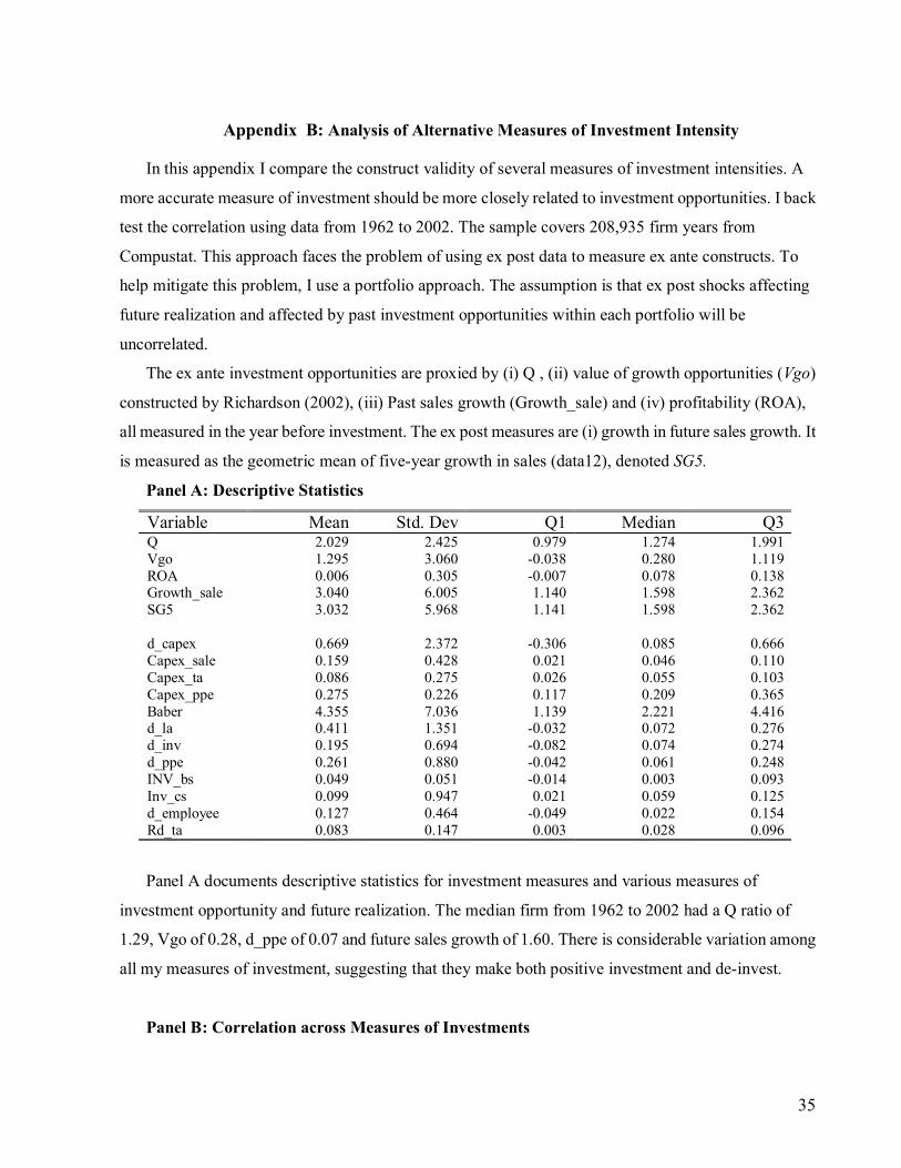
35

Appendix B: Analysis of Alternative Measures of Investment Intensity

In this appendix I compare the construct validity of several measures of investment intensities. A

more accurate measure of investment should be more closely related to investment opportunities. I back

test the correlation using data from 1962 to 2002. The sample covers 208,935 firm years from

Compustat. This approach faces the problem of using ex post data to measure ex ante constructs. To

help mitigate this problem, I use a portfolio approach. The assumption is that ex post shocks affecting

future realization and affected by past investment opportunities within each portfolio will be

uncorrelated.

The ex ante investment opportunities are proxied by (i) Q , (ii) value of growth opportunities (Vgo)

constructed by Richardson (2002), (iii) Past sales growth (Growth_sale) and (iv) profitability (ROA),

all measured in the year before investment. The ex post measures are (i) growth in future sales growth. It

is measured as the geometric mean of five-year growth in sales (data12), denoted SG5.

Panel A: Descriptive Statistics

Variable Mean Std. Dev Q1 Median Q3Q 2.029 2.425 0.979 1.274 1.991 Vgo 1.295 3.060 -0.038 0.280 1.119 ROA 0.006 0.305 -0.007 0.078 0.138 Growth_sale 3.040 6.005 1.140 1.598 2.362 SG5 3.032 5.968 1.141 1.598 2.362 d_capex 0.669 2.372 -0.306 0.085 0.666 Capex_sale 0.159 0.428 0.021 0.046 0.110 Capex_ta 0.086 0.275 0.026 0.055 0.103 Capex_ppe 0.275 0.226 0.117 0.209 0.365 Baber 4.355 7.036 1.139 2.221 4.416 d_la 0.411 1.351 -0.032 0.072 0.276 d_inv 0.195 0.694 -0.082 0.074 0.274 d_ppe 0.261 0.880 -0.042 0.061 0.248 INV_bs 0.049 0.051 -0.014 0.003 0.093 Inv_cs 0.099 0.947 0.021 0.059 0.125 d_employee 0.127 0.464 -0.049 0.022 0.154 Rd_ta 0.083 0.147 0.003 0.028 0.096 Panel A documents descriptive statistics for investment measures and various measures of

investment opportunity and future realization. The median firm from 1962 to 2002 had a Q ratio of

1.29, Vgo of 0.28, d_ppe of 0.07 and future sales growth of 1.60. There is considerable variation among

all my measures of investment, suggesting that they make both positive investment and de-invest.

Panel B: Correlation across Measures of Investments

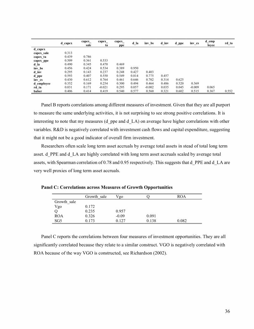
36

Panel B reports correlations among different measures of investment. Given that they are all purport

to measure the same underlying activities, it is not surprising to see strong positive correlations. It is

interesting to note that my measures (d_ppe and d_LA) on average have higher correlations with other

variables. R&D is negatively correlated with investment cash flows and capital expenditure, suggesting

that it might not be a good indicator of overall firm investment.

Researchers often scale long term asset accruals by average total assets in stead of total long term

asset. d_PPE and d_LA are highly correlated with long term asset accruals scaled by average total

assets, with Spearman correlation of 0.78 and 0.95 respectively. This suggests that d_PPE and d_LA are

very well proxies of long term asset accruals.

Panel C: Correlations across Measures of Growth Opportunities

Panel C reports the correlations between four measures of investment opportunities. They are all

significantly correlated because they relate to a similar construct. VGO is negatively correlated with

ROA because of the way VGO is constructed, see Richardson (2002).

d_capex capex_ sale

capex_ ta

capex_ ppe d_la inv_bs d_inv d_ppe inv_cs d_emp

loyee rd_ta

d_capex capex_sale 0.313 capex_ta 0.439 0.786 capex_ppe 0.509 0.361 0.533 d_la 0.490 0.345 0.470 0.469 inv_bs 0.456 0.424 0.534 0.389 0.950 d_inv 0.295 0.143 0.237 0.248 0.427 0.403 d_ppe 0.593 0.407 0.550 0.549 0.814 0.775 0.457 inv_cs 0.430 0.612 0.764 0.461 0.646 0.702 0.314 0.625 d_employee 0.352 0.169 0.254 0.300 0.494 0.464 0.486 0.520 0.369 rd_ta 0.031 0.171 -0.021 0.295 0.057 -0.002 0.035 0.045 -0.009 0.065 baber 0.406 0.414 0.419 0.540 0.577 0.560 0.321 0.602 0.515 0.367 0.552

Growth_sale Vgo Q ROA Growth_sale Vgo 0.172 Q 0.235 0.957 ROA 0.326 -0.09 0.091 SG5 0.173 0.127 0.138 0.082

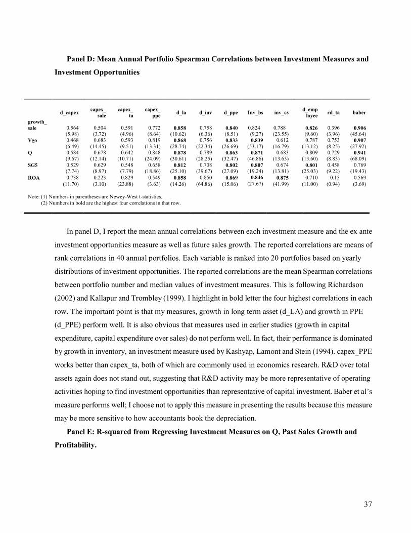
37

Panel D: Mean Annual Portfolio Spearman Correlations between Investment Measures and

Investment Opportunities

In panel D, I report the mean annual correlations between each investment measure and the ex ante

investment opportunities measure as well as future sales growth. The reported correlations are means of

rank correlations in 40 annual portfolios. Each variable is ranked into 20 portfolios based on yearly

distributions of investment opportunities. The reported correlations are the mean Spearman correlations

between portfolio number and median values of investment measures. This is following Richardson

(2002) and Kallapur and Trombley (1999). I highlight in bold letter the four highest correlations in each

row. The important point is that my measures, growth in long term asset (d_LA) and growth in PPE

(d_PPE) perform well. It is also obvious that measures used in earlier studies (growth in capital

expenditure, capital expenditure over sales) do not perform well. In fact, their performance is dominated

by growth in inventory, an investment measure used by Kashyap, Lamont and Stein (1994). capex_PPE

works better than capex_ta, both of which are commonly used in economics research. R&D over total

assets again does not stand out, suggesting that R&D activity may be more representative of operating

activities hoping to find investment opportunities than representative of capital investment. Baber et al’s

measure performs well; I choose not to apply this measure in presenting the results because this measure

may be more sensitive to how accountants book the depreciation.

Panel E: R-squared from Regressing Investment Measures on Q, Past Sales Growth and

Profitability.

d_capex capex_ sale

capex_ ta

capex_ ppe d_la d_inv d_ppe Inv_bs inv_cs d_emp

loyee rd_ta baber

growth_sale 0.564 0.504 0.591 0.772 0.858 0.758 0.840 0.824 0.788 0.826 0.396 0.906 (5.98) (3.72) (4.96) (8.64) (10.62) (6.36) (8.51) (9.27) (23.55) (9.60) (3.96) (45.64) Vgo 0.468 0.683 0.593 0.819 0.868 0.756 0.833 0.839 0.612 0.787 0.753 0.907 (6.49) (14.45) (9.51) (13.31) (28.74) (22.34) (26.69) (53.17) (16.79) (13.12) (8.25) (27.92) Q 0.584 0.678 0.642 0.848 0.878 0.789 0.863 0.871 0.683 0.809 0.729 0.941 (9.67) (12.14) (10.71) (24.09) (30.61) (28.25) (32.47) (46.86) (13.63) (13.60) (8.83) (68.09) SG5 0.529 0.629 0.548 0.658 0.812 0.708 0.802 0.807 0.674 0.801 0.458 0.769 (7.74) (8.97) (7.79) (18.86) (25.10) (39.67) (27.09) (19.24) (13.81) (25.03) (9.22) (19.43) ROA 0.738 0.223 0.829 0.549 0.858 0.850 0.869 0.846 0.875 0.710 0.15 0.569 (11.70) (3.10) (23.88) (3.63) (14.26) (64.86) (15.06) (27.67) (41.99) (11.00) (0.94) (3.69) Note: (1) Numbers in parentheses are Newey-West t-statistics. (2) Numbers in bold are the highest four correlations in that row.

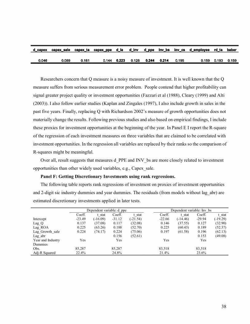
38

Researchers concern that Q measure is a noisy measure of investment. It is well known that the Q

measure suffers from serious measurement error problem. People contend that higher profitability can

signal greater project quality or investment opportunities (Fazzari et al (1988), Cleary (1999) and Alti

(2003)). I also follow earlier studies (Kaplan and Zingales (1997), I also include growth in sales in the

past five years. Finally, replacing Q with Richardson 2002’s measure of growth opportunities does not

materially change the results. Following previous studies and also based on empirical findings, I include

these proxies for investment opportunities at the beginning of the year. In Panel E I report the R-square

of the regression of each investment measures on three variables that are claimed to be correlated with

investment opportunities. In the regression all variables are replaced by their ranks so the comparison of

R-squares might be meaningful.

Over all, result suggests that measures d_PPE and INV_bs are more closely related to investment

opportunities than other widely used variables, e.g., Capex_sale.

Panel F: Getting Discretionary Investments using rank regressions.

The following table reports rank regressions of investment on proxies of investment opportunities

and 2-digit sic industry dummies and year dummies. The residuals (from models without lag_abr) are

estimated discretionary investments applied in later tests.

d_capex capex_sale capex_ta capex_ppe d_la d_inv d_ppe Inv_bs inv_cs d_employee rd_ta baber

0.046 0.089 0.161 0.144 0.223 0.128 0.244 0.214 0.195 0.159 0.193 0.159

d_capex capex_sale capex_ta capex_ppe d_la d_inv d_ppe Inv_bs inv_cs d_employee rd_ta baber

0.046 0.089 0.161 0.144 0.223 0.128 0.244 0.214 0.195 0.159 0.193 0.159

Dependent variable: d_ppe Dependent variable: Inv_bs Coeff. t_stat Coeff. t_stat Coeff. t_stat Coeff. t_stat Intercept -23.49 (-16.09) -31.12 (-21.54) -22.66 (-14.46) -29.94 (-19.29) Lag_Q 0.137 (37.08) 0.117 (32.08) 0.146 (37.55) 0.127 (32.90) Lag_ROA 0.225 (63.26) 0.188 (52.70) 0.225 (60.43) 0.189 (52.37) Lag_Growth_sale 0.224 (74.17) 0.224 (75.06) 0.197 (61.58) 0.196 (62.13) Lag_abr 0.156 (52.61) 0.153 (49.08) Year and Industry Dummies

Yes Yes Yes Yes

Obs. 85,287 85,287 83,518 83,518 Adj-R Squared 22.4% 24.8% 21.4% 23.6%

d_capex capex_sale capex_ta capex_ppe d_la d_inv d_ppe Inv_bs inv_cs d_employee rd_ta baber

0.046 0.089 0.161 0.144 0.223 0.128 0.244 0.214 0.195 0.159 0.193 0.159

d_capex capex_sale capex_ta capex_ppe d_la d_inv d_ppe Inv_bs inv_cs d_employee rd_ta baber

0.046 0.089 0.161 0.144 0.223 0.128 0.244 0.214 0.195 0.159 0.193 0.159

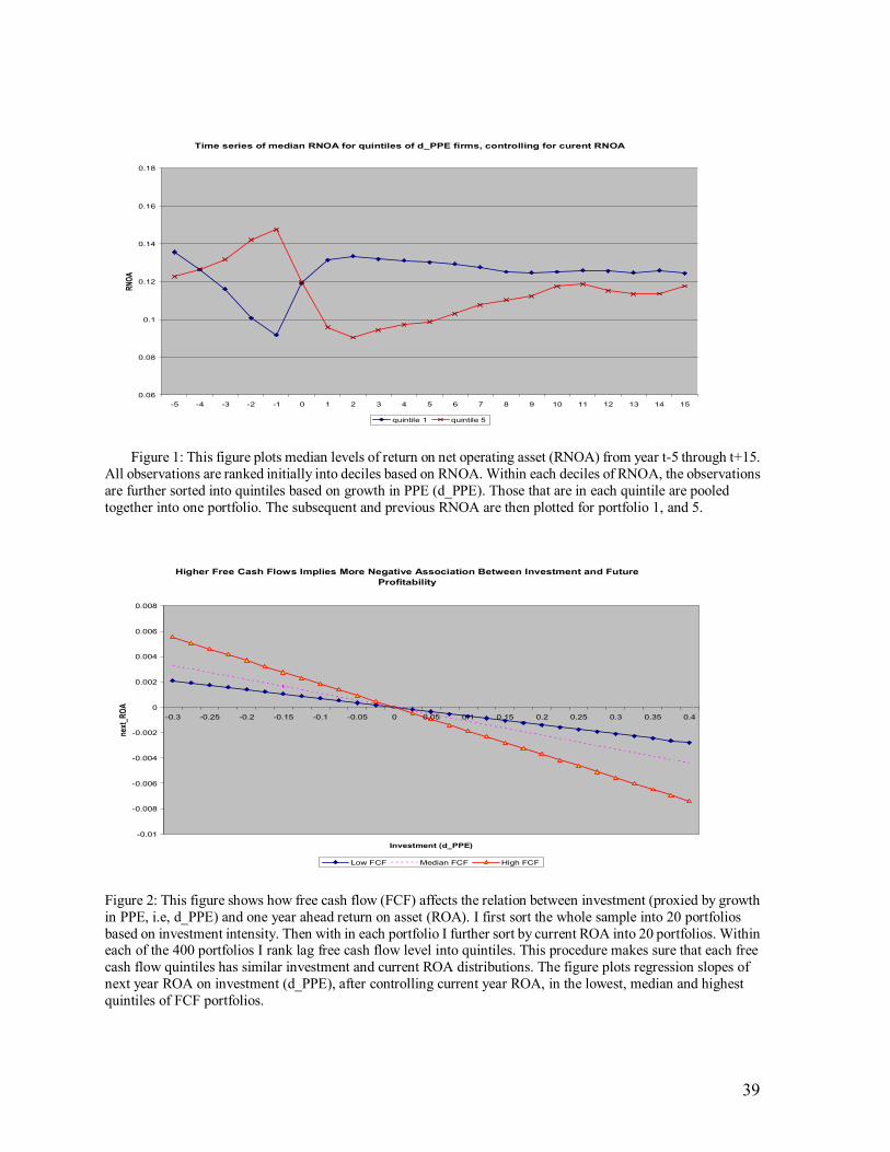
39

Time series of median RNOA for quintiles of d_PPE firms, controlling for curent RNOA

0.06

0.08

0.1

0.12

0.14

0.16

0.18

-5 -4 -3 -2 -1 0 1 2 3 4 5 6 7 8 9 10 11 12 13 14 15

RNOA

quintile 1 quintile 5 Figure 1: This figure plots median levels of return on net operating asset (RNOA) from year t-5 through t+15.

All observations are ranked initially into deciles based on RNOA. Within each deciles of RNOA, the observations are further sorted into quintiles based on growth in PPE (d_PPE). Those that are in each quintile are pooled together into one portfolio. The subsequent and previous RNOA are then plotted for portfolio 1, and 5.

Higher Free Cash Flows Implies More Negative Association Between Investment and Future Profitability

-0.01

-0.008

-0.006

-0.004

-0.002

0

0.002

0.004

0.006

0.008

-0.3 -0.25 -0.2 -0.15 -0.1 -0.05 0 0.05 0.1 0.15 0.2 0.25 0.3 0.35 0.4

Investment (d_PPE)

next_

ROA

Low FCF Median FCF High FCF

Figure 2: This figure shows how free cash flow (FCF) affects the relation between investment (proxied by growth in PPE, i.e, d_PPE) and one year ahead return on asset (ROA). I first sort the whole sample into 20 portfolios based on investment intensity. Then with in each portfolio I further sort by current ROA into 20 portfolios. Within each of the 400 portfolios I rank lag free cash flow level into quintiles. This procedure makes sure that each free cash flow quintiles has similar investment and current ROA distributions. The figure plots regression slopes of next year ROA on investment (d_PPE), after controlling current year ROA, in the lowest, median and highest quintiles of FCF portfolios.

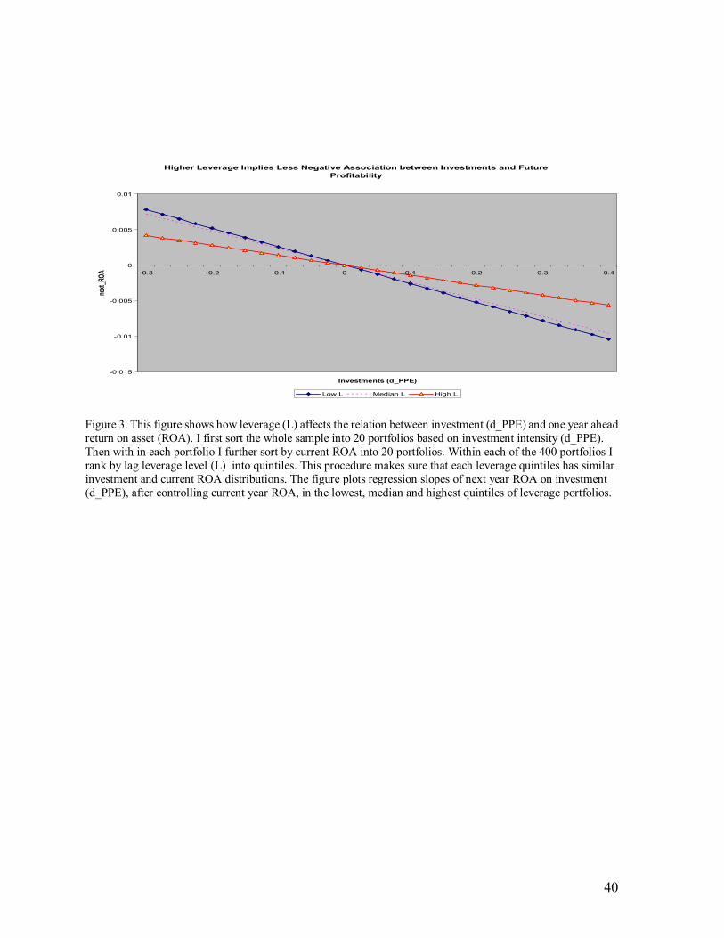
40

Higher Leverage Implies Less Negative Association between Investments and Future Profitability

-0.015

-0.01

-0.005

0

0.005

0.01

-0.3 -0.2 -0.1 0 0.1 0.2 0.3 0.4

Investments (d_PPE)

next_

ROA

Low L Median L High L Figure 3. This figure shows how leverage (L) affects the relation between investment (d_PPE) and one year ahead return on asset (ROA). I first sort the whole sample into 20 portfolios based on investment intensity (d_PPE). Then with in each portfolio I further sort by current ROA into 20 portfolios. Within each of the 400 portfolios I rank by lag leverage level (L) into quintiles. This procedure makes sure that each leverage quintiles has similar investment and current ROA distributions. The figure plots regression slopes of next year ROA on investment (d_PPE), after controlling current year ROA, in the lowest, median and highest quintiles of leverage portfolios.

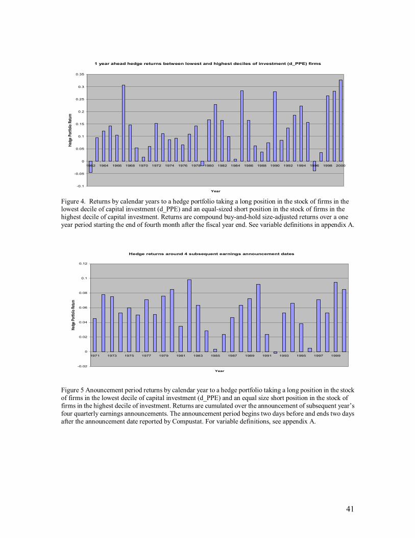
41

1 year ahead hedge returns between lowest and highest deciles of investment (d_PPE) firms

-0.1

-0.05

0

0.05

0.1

0.15

0.2

0.25

0.3

0.35

1962 1964 1966 1968 1970 1972 1974 1976 1978 1980 1982 1984 1986 1988 1990 1992 1994 1996 1998 2000

Year

Hedg

e Port

folio

Retur

n

Figure 4. Returns by calendar years to a hedge portfolio taking a long position in the stock of firms in the lowest decile of capital investment (d_PPE) and an equal-sized short position in the stock of firms in the highest decile of capital investment. Returns are compound buy-and-hold size-adjusted returns over a one year period starting the end of fourth month after the fiscal year end. See variable definitions in appendix A.

Hedge returns around 4 subsequent earnings announcement dates

-0.02

0

0.02

0.04

0.06

0.08

0.1

0.12

1971 1973 1975 1977 1979 1981 1983 1985 1987 1989 1991 1993 1995 1997 1999

Year

Hedg

e Port

folio

Retur

n

Figure 5 Anouncement period returns by calendar year to a hedge portfolio taking a long position in the stock of firms in the lowest decile of capital investment (d_PPE) and an equal size short position in the stock of firms in the highest decile of investment. Returns are cumulated over the announcement of subsequent year’s four quarterly earnings announcements. The announcement period begins two days before and ends two days after the announcement date reported by Compustat. For variable definitions, see appendix A.

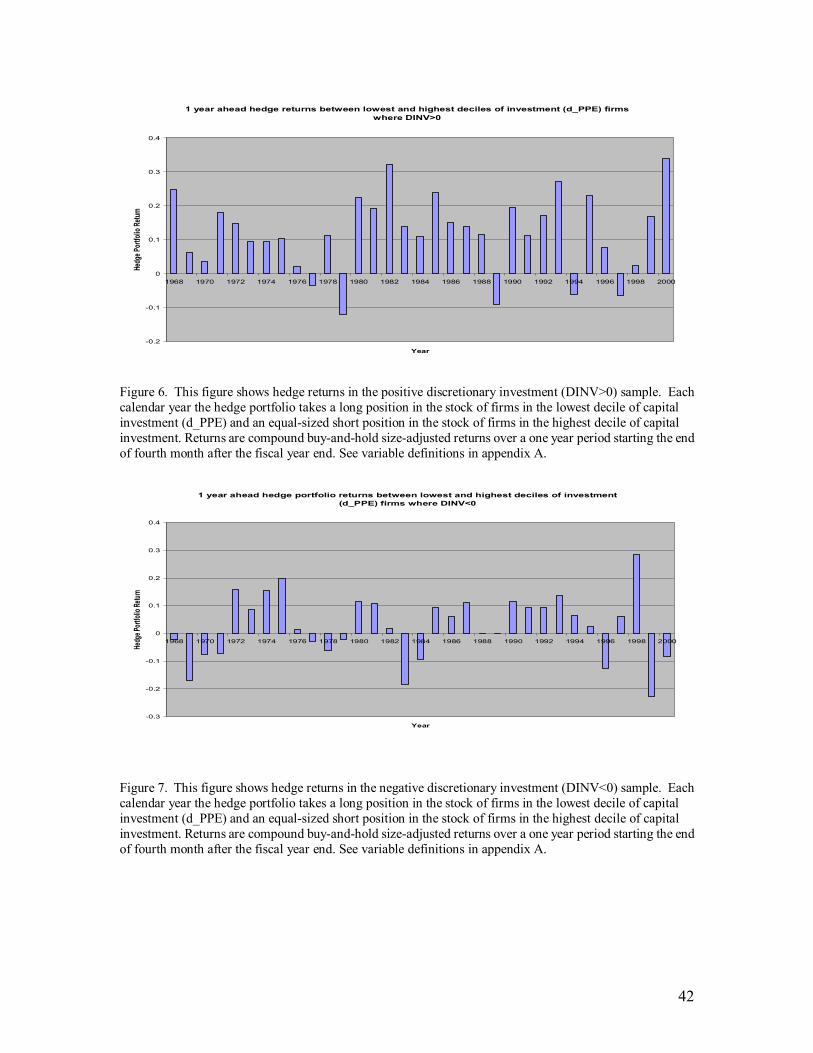
42

1 year ahead hedge returns between lowest and highest deciles of investment (d_PPE) firms where DINV>0

-0.2

-0.1

0

0.1

0.2

0.3

0.4

1968 1970 1972 1974 1976 1978 1980 1982 1984 1986 1988 1990 1992 1994 1996 1998 2000

Year

Hedg

e Port

folio

Retur

n

Figure 6. This figure shows hedge returns in the positive discretionary investment (DINV>0) sample. Each calendar year the hedge portfolio takes a long position in the stock of firms in the lowest decile of capital investment (d_PPE) and an equal-sized short position in the stock of firms in the highest decile of capital investment. Returns are compound buy-and-hold size-adjusted returns over a one year period starting the end of fourth month after the fiscal year end. See variable definitions in appendix A.

1 year ahead hedge portfolio returns between lowest and highest deciles of investment

(d_PPE) firms where DINV<0

-0.3

-0.2

-0.1

0

0.1

0.2

0.3

0.4

1968 1970 1972 1974 1976 1978 1980 1982 1984 1986 1988 1990 1992 1994 1996 1998 2000

Year

Hedg

e Port

folio

Retur

n

Figure 7. This figure shows hedge returns in the negative discretionary investment (DINV<0) sample. Each calendar year the hedge portfolio takes a long position in the stock of firms in the lowest decile of capital investment (d_PPE) and an equal-sized short position in the stock of firms in the highest decile of capital investment. Returns are compound buy-and-hold size-adjusted returns over a one year period starting the end of fourth month after the fiscal year end. See variable definitions in appendix A.

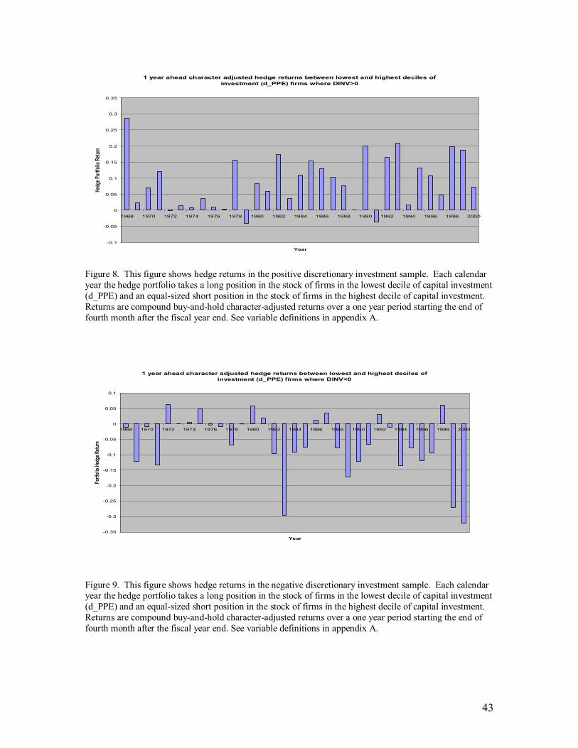
43

1 year ahead character adjusted hedge returns between lowest and highest deciles of investment (d_PPE) firms where DINV>0

-0.1

-0.05

0

0.05

0.1

0.15

0.2

0.25

0.3

0.35

1968 1970 1972 1974 1976 1978 1980 1982 1984 1986 1988 1990 1992 1994 1996 1998 2000

Year

Hedg

e Port

folio

Retur

n

Figure 8. This figure shows hedge returns in the positive discretionary investment sample. Each calendar year the hedge portfolio takes a long position in the stock of firms in the lowest decile of capital investment (d_PPE) and an equal-sized short position in the stock of firms in the highest decile of capital investment. Returns are compound buy-and-hold character-adjusted returns over a one year period starting the end of fourth month after the fiscal year end. See variable definitions in appendix A.

1 year ahead character adjusted hedge returns between lowest and highest deciles of investment (d_PPE) firms where DINV<0

-0.35

-0.3

-0.25

-0.2

-0.15

-0.1

-0.05

0

0.05

0.1

1968 1970 1972 1974 1976 1978 1980 1982 1984 1986 1988 1990 1992 1994 1996 1998 2000

Year

Portfo

lio He

dge R

eturn

Figure 9. This figure shows hedge returns in the negative discretionary investment sample. Each calendar year the hedge portfolio takes a long position in the stock of firms in the lowest decile of capital investment (d_PPE) and an equal-sized short position in the stock of firms in the highest decile of capital investment. Returns are compound buy-and-hold character-adjusted returns over a one year period starting the end of fourth month after the fiscal year end. See variable definitions in appendix A.

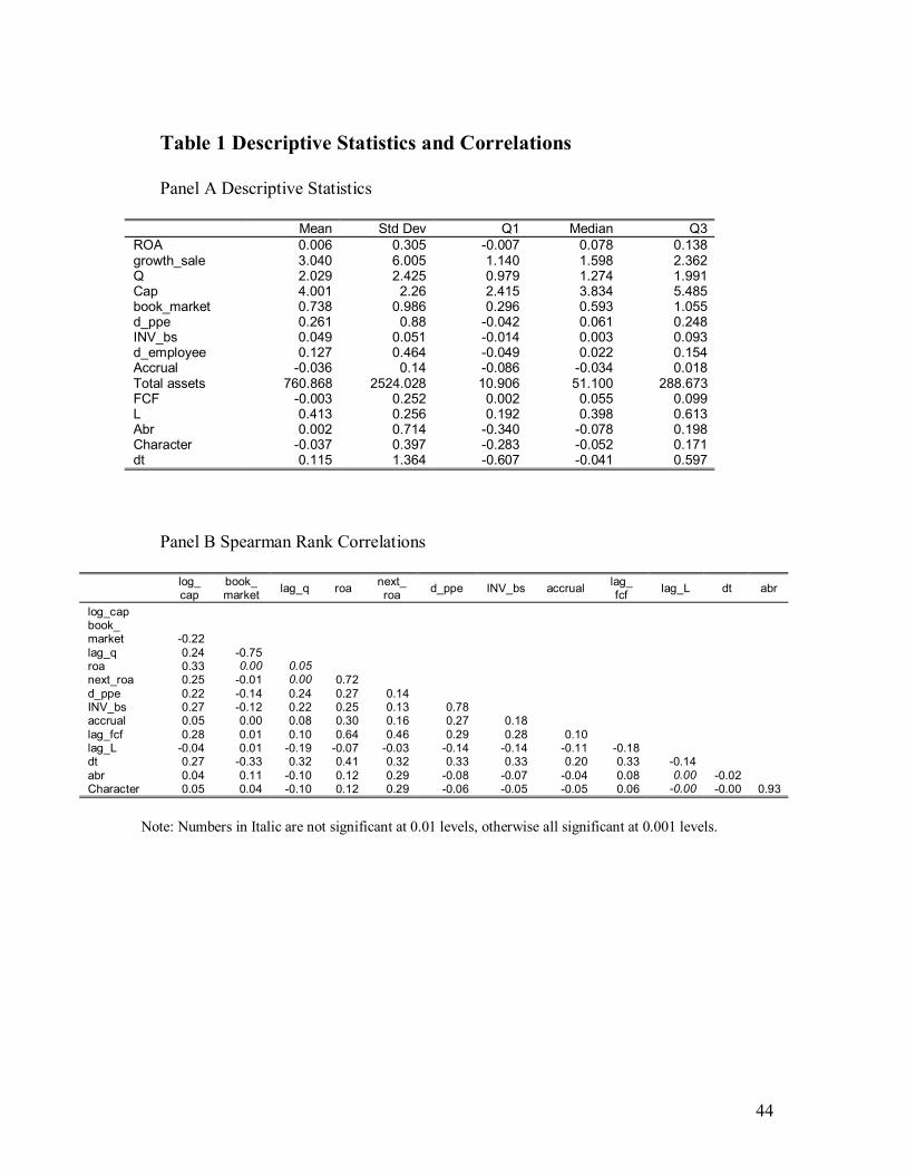
44

Table 1 Descriptive Statistics and Correlations Panel A Descriptive Statistics

Mean Std Dev Q1 Median Q3 ROA 0.006 0.305 -0.007 0.078 0.138 growth_sale 3.040 6.005 1.140 1.598 2.362 Q 2.029 2.425 0.979 1.274 1.991 Cap 4.001 2.26 2.415 3.834 5.485 book_market 0.738 0.986 0.296 0.593 1.055 d_ppe 0.261 0.88 -0.042 0.061 0.248 INV_bs 0.049 0.051 -0.014 0.003 0.093 d_employee 0.127 0.464 -0.049 0.022 0.154 Accrual -0.036 0.14 -0.086 -0.034 0.018 Total assets 760.868 2524.028 10.906 51.100 288.673 FCF -0.003 0.252 0.002 0.055 0.099 L 0.413 0.256 0.192 0.398 0.613 Abr 0.002 0.714 -0.340 -0.078 0.198 Character -0.037 0.397 -0.283 -0.052 0.171 dt 0.115 1.364 -0.607 -0.041 0.597

Panel B Spearman Rank Correlations

log_ cap

book_market lag_q roa next_

roa d_ppe INV_bs accrual lag_ fcf lag_L dt abr

log_cap book_ market -0.22

lag_q 0.24 -0.75 roa 0.33 0.00 0.05 next_roa 0.25 -0.01 0.00 0.72 d_ppe 0.22 -0.14 0.24 0.27 0.14 INV_bs 0.27 -0.12 0.22 0.25 0.13 0.78 accrual 0.05 0.00 0.08 0.30 0.16 0.27 0.18 lag_fcf 0.28 0.01 0.10 0.64 0.46 0.29 0.28 0.10 lag_L -0.04 0.01 -0.19 -0.07 -0.03 -0.14 -0.14 -0.11 -0.18 dt 0.27 -0.33 0.32 0.41 0.32 0.33 0.33 0.20 0.33 -0.14 abr 0.04 0.11 -0.10 0.12 0.29 -0.08 -0.07 -0.04 0.08 0.00 -0.02 Character 0.05 0.04 -0.10 0.12 0.29 -0.06 -0.05 -0.05 0.06 -0.00 -0.00 0.93

Note: Numbers in Italic are not significant at 0.01 levels, otherwise all significant at 0.001 levels.

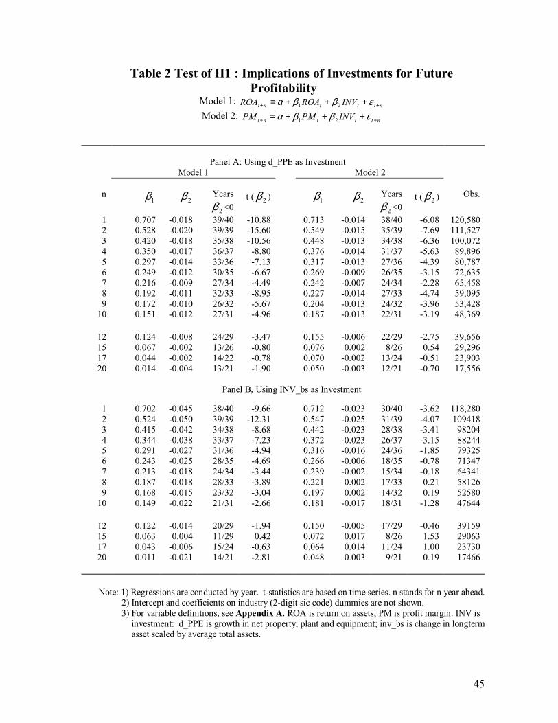
45

Table 2 Test of H1 : Implications of Investments for Future Profitability

Model 1: ntttnt INVROAROA ++ +++= εββα 21 Model 2: ntttnt INVPMPM ++ +++= εββα 21

Panel B, Using INV_bs as Investment

Note: 1) Regressions are conducted by year. t-statistics are based on time series. n stands for n year ahead. 2) Intercept and coefficients on industry (2-digit sic code) dummies are not shown. 3) For variable definitions, see Appendix A. ROA is return on assets; PM is profit margin. INV is

investment: d_PPE is growth in net property, plant and equipment; inv_bs is change in longterm asset scaled by average total assets.

Panel A: Using d_PPE as Investment Model 1 Model 2

n 1β 2β Years

2β <0 t ( 2β ) 1β 2β Years

2β <0 t ( 2β ) Obs.

1 0.707 -0.018 39/40 -10.88 0.713 -0.014 38/40 -6.08 120,580 2 0.528 -0.020 39/39 -15.60 0.549 -0.015 35/39 -7.69 111,527 3 0.420 -0.018 35/38 -10.56 0.448 -0.013 34/38 -6.36 100,072 4 0.350 -0.017 36/37 -8.80 0.376 -0.014 31/37 -5.63 89,896 5 0.297 -0.014 33/36 -7.13 0.317 -0.013 27/36 -4.39 80,787 6 0.249 -0.012 30/35 -6.67 0.269 -0.009 26/35 -3.15 72,635 7 0.216 -0.009 27/34 -4.49 0.242 -0.007 24/34 -2.28 65,458 8 0.192 -0.011 32/33 -8.95 0.227 -0.014 27/33 -4.74 59,095 9 0.172 -0.010 26/32 -5.67 0.204 -0.013 24/32 -3.96 53,428

10 0.151 -0.012 27/31 -4.96 0.187 -0.013 22/31 -3.19 48,369

12 0.124 -0.008 24/29 -3.47 0.155 -0.006 22/29 -2.75 39,656 15 0.067 -0.002 13/26 -0.80 0.076 0.002 8/26 0.54 29,296 17 0.044 -0.002 14/22 -0.78 0.070 -0.002 13/24 -0.51 23,903 20 0.014 -0.004 13/21 -1.90 0.050 -0.003 12/21 -0.70 17,556

1 0.702 -0.045 38/40 -9.66 0.712 -0.023 30/40 -3.62 118,2802 0.524 -0.050 39/39 -12.31 0.547 -0.025 31/39 -4.07 109418 3 0.415 -0.042 34/38 -8.68 0.442 -0.023 28/38 -3.41 98204 4 0.344 -0.038 33/37 -7.23 0.372 -0.023 26/37 -3.15 88244 5 0.291 -0.027 31/36 -4.94 0.316 -0.016 24/36 -1.85 79325 6 0.243 -0.025 28/35 -4.69 0.266 -0.006 18/35 -0.78 71347 7 0.213 -0.018 24/34 -3.44 0.239 -0.002 15/34 -0.18 64341 8 0.187 -0.018 28/33 -3.89 0.221 0.002 17/33 0.21 58126 9 0.168 -0.015 23/32 -3.04 0.197 0.002 14/32 0.19 52580

10 0.149 -0.022 21/31 -2.66 0.181 -0.017 18/31 -1.28 47644

12 0.122 -0.014 20/29 -1.94 0.150 -0.005 17/29 -0.46 39159 15 0.063 0.004 11/29 0.42 0.072 0.017 8/26 1.53 29063 17 0.043 -0.006 15/24 -0.63 0.064 0.014 11/24 1.00 23730 20 0.011 -0.021 14/21 -2.81 0.048 0.003 9/21 0.19 17466

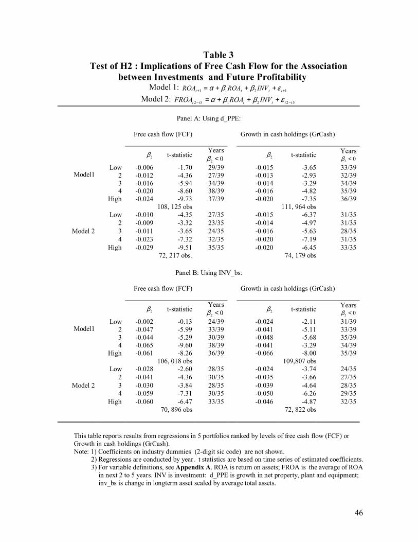
46

Table 3 Test of H2 : Implications of Free Cash Flow for the Association

between Investments and Future Profitability Model 1: 1211 ++ +++= tttt INVROAROA εββα

Model 2: 522152 tttttt INVROAFROA −− +++= εββα

Panel A: Using d_PPE:

Free cash flow (FCF)

Growth in cash holdings (GrCash)

2β t-statistic

Years 02 <β 2β t-statistic Years

02 <βLow -0.006 -1.70 29/39 -0.015 -3.65 33/39

2 -0.012 -4.36 27/39 -0.013 -2.93 32/39 3 -0.016 -5.94 34/39 -0.014 -3.29 34/39 4 -0.020 -8.60 38/39 -0.016 -4.82 35/39

Model1

High -0.024 -9.73 37/39 -0.020 -7.35 36/39 108, 125 obs 111, 964 obs

Low -0.010 -4.35 27/35 -0.015 -6.37 31/35 2 -0.009 -3.32 23/35 -0.014 -4.97 31/35 3 -0.011 -3.65 24/35 -0.016 -5.63 28/35 4 -0.023 -7.32 32/35 -0.020 -7.19 31/35

Model 2

High -0.029 -9.51 35/35 -0.020 -6.45 33/35 72, 217 obs. 74, 179 obs

Panel B: Using INV_bs:

Free cash flow (FCF)

Growth in cash holdings (GrCash)

2β t-statistic Years

02 <β 2β t-statistic Years 02 <β

Low -0.002 -0.13 24/39 -0.024 -2.11 31/39 2 -0.047 -5.99 33/39 -0.041 -5.11 33/39 3 -0.044 -5.29 30/39 -0.048 -5.68 35/39 4 -0.065 -9.60 38/39 -0.041 -3.29 34/39

Model1

High -0.061 -8.26 36/39 -0.066 -8.00 35/39 106, 018 obs 109,807 obs

Low -0.028 -2.60 28/35 -0.024 -3.74 24/35 2 -0.041 -4.36 30/35 -0.035 -3.66 27/35 3 -0.030 -3.84 28/35 -0.039 -4.64 28/35 4 -0.059 -7.31 30/35 -0.050 -6.26 29/35

Model 2

High -0.060 -6.47 33/35 -0.046 -4.87 32/35 70, 896 obs 72, 822 obs

This table reports results from regressions in 5 portfolios ranked by levels of free cash flow (FCF) or Growth in cash holdings (GrCash). Note: 1) Coefficients on industry dummies (2-digit sic code) are not shown. 2) Regressions are conducted by year. t statistics are based on time series of estimated coefficients. 3) For variable definitions, see Appendix A. ROA is return on assets; FROA is the average of ROA

in next 2 to 5 years. INV is investment: d_PPE is growth in net property, plant and equipment; inv_bs is change in longterm asset scaled by average total assets.

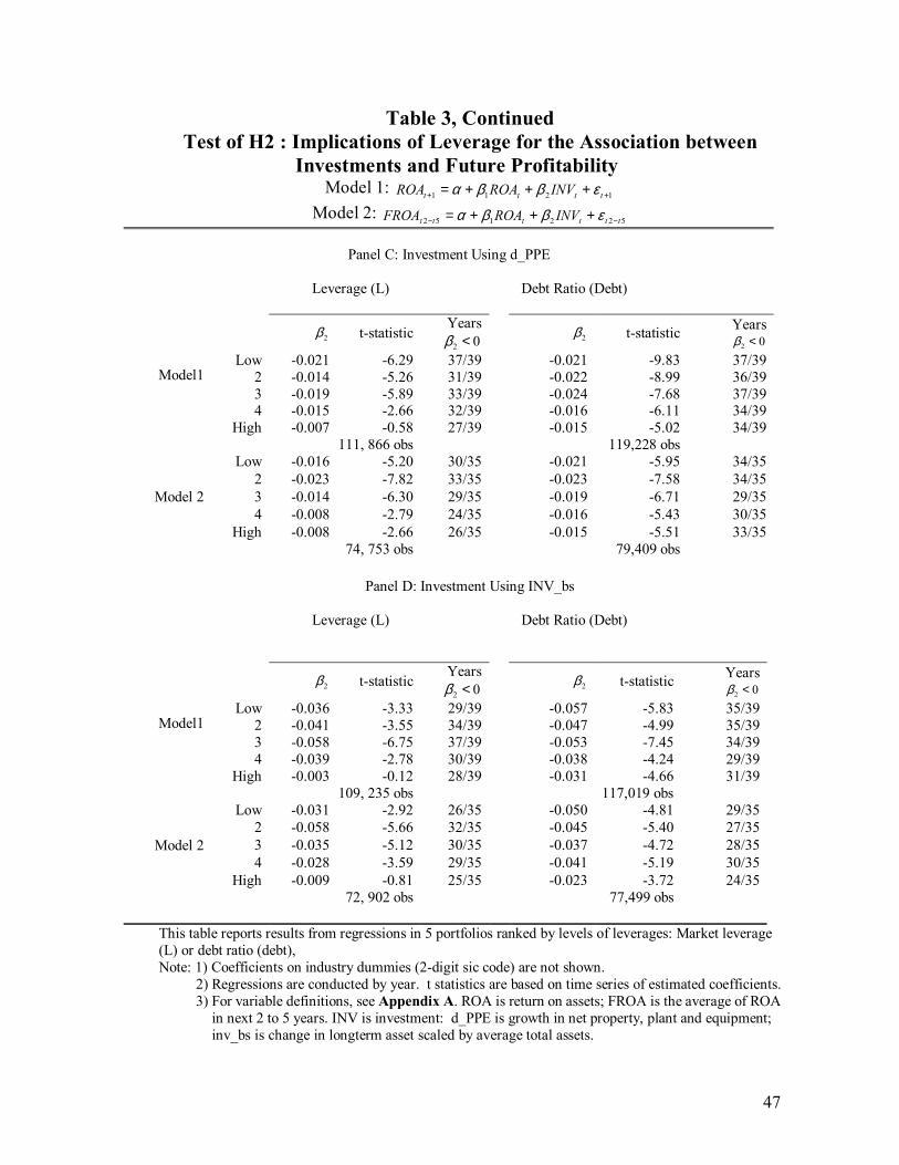
47

Table 3, Continued Test of H2 : Implications of Leverage for the Association between

Investments and Future Profitability Model 1: 1211 ++ +++= tttt INVROAROA εββα

Model 2: 522152 tttttt INVROAFROA −− +++= εββα

Panel C: Investment Using d_PPE

Leverage (L)

Debt Ratio (Debt)

2β t-statistic

Years 02 <β 2β t-statistic Years

02 <βLow -0.021 -6.29 37/39 -0.021 -9.83 37/39

2 -0.014 -5.26 31/39 -0.022 -8.99 36/39 3 -0.019 -5.89 33/39 -0.024 -7.68 37/39 4 -0.015 -2.66 32/39 -0.016 -6.11 34/39

Model1

High -0.007 -0.58 27/39 -0.015 -5.02 34/39 111, 866 obs 119,228 obs

Low -0.016 -5.20 30/35 -0.021 -5.95 34/35 2 -0.023 -7.82 33/35 -0.023 -7.58 34/35 3 -0.014 -6.30 29/35 -0.019 -6.71 29/35 4 -0.008 -2.79 24/35 -0.016 -5.43 30/35

Model 2

High -0.008 -2.66 26/35 -0.015 -5.51 33/35 74, 753 obs 79,409 obs

Panel D: Investment Using INV_bs

Leverage (L)

Debt Ratio (Debt)

2β t-statistic

Years 02 <β 2β t-statistic Years

02 <βLow -0.036 -3.33 29/39 -0.057 -5.83 35/39

2 -0.041 -3.55 34/39 -0.047 -4.99 35/39 3 -0.058 -6.75 37/39 -0.053 -7.45 34/39 4 -0.039 -2.78 30/39 -0.038 -4.24 29/39

Model1

High -0.003 -0.12 28/39 -0.031 -4.66 31/39 109, 235 obs 117,019 obs

Low -0.031 -2.92 26/35 -0.050 -4.81 29/35 2 -0.058 -5.66 32/35 -0.045 -5.40 27/35 3 -0.035 -5.12 30/35 -0.037 -4.72 28/35 4 -0.028 -3.59 29/35 -0.041 -5.19 30/35

Model 2

High -0.009 -0.81 25/35 -0.023 -3.72 24/35 72, 902 obs 77,499 obs

This table reports results from regressions in 5 portfolios ranked by levels of leverages: Market leverage (L) or debt ratio (debt), Note: 1) Coefficients on industry dummies (2-digit sic code) are not shown. 2) Regressions are conducted by year. t statistics are based on time series of estimated coefficients. 3) For variable definitions, see Appendix A. ROA is return on assets; FROA is the average of ROA

in next 2 to 5 years. INV is investment: d_PPE is growth in net property, plant and equipment; inv_bs is change in longterm asset scaled by average total assets.

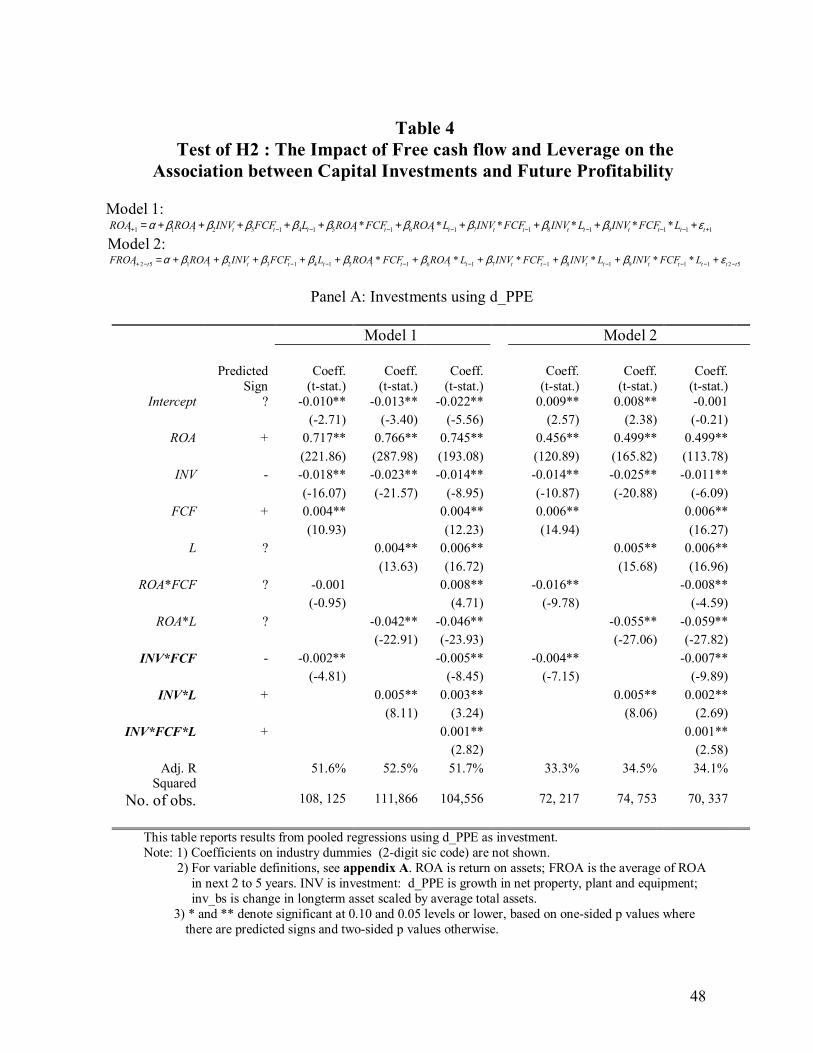
48

Table 4

Test of H2 : The Impact of Free cash flow and Leverage on the Association between Capital Investments and Future Profitability

Model 1:

1119181716151413211 ****** +−−−−−−−−+ ++++++++++= ttttttttttttttttt LFCFINVLINVFCFINVLROAFCFROALFCFINVROAROA εβββββββββα

Model 2: 521191817161514132152 ****** ttttttttttttttttttt LFCFINVLINVFCFINVLROAFCFROALFCFINVROAFROA −−−−−−−−−−+ ++++++++++= εβββββββββα

Panel A: Investments using d_PPE

Model 1 Model 2 Predicted

Sign Coeff.

(t-stat.) Coeff.

(t-stat.) Coeff.

(t-stat.) Coeff.

(t-stat.) Coeff.

(t-stat.) Coeff.

(t-stat.) Intercept ? -0.010** -0.013** -0.022** 0.009** 0.008** -0.001

(-2.71) (-3.40) (-5.56) (2.57) (2.38) (-0.21) ROA + 0.717** 0.766** 0.745** 0.456** 0.499** 0.499**

(221.86) (287.98) (193.08) (120.89) (165.82) (113.78) INV - -0.018** -0.023** -0.014** -0.014** -0.025** -0.011**

(-16.07) (-21.57) (-8.95) (-10.87) (-20.88) (-6.09) FCF + 0.004** 0.004** 0.006** 0.006**

(10.93) (12.23) (14.94) (16.27) L ? 0.004** 0.006** 0.005** 0.006**

(13.63) (16.72) (15.68) (16.96) ROA*FCF ? -0.001 0.008** -0.016** -0.008**

(-0.95) (4.71) (-9.78) (-4.59) ROA*L ? -0.042** -0.046** -0.055** -0.059**

(-22.91) (-23.93) (-27.06) (-27.82) INV*FCF - -0.002** -0.005** -0.004** -0.007**

(-4.81) (-8.45) (-7.15) (-9.89) INV*L + 0.005** 0.003** 0.005** 0.002**

(8.11) (3.24) (8.06) (2.69) INV*FCF*L + 0.001** 0.001**

(2.82) (2.58) Adj. R

Squared 51.6% 52.5% 51.7% 33.3% 34.5% 34.1%

No. of obs. 108, 125 111,866 104,556 72, 217 74, 753 70, 337

This table reports results from pooled regressions using d_PPE as investment. Note: 1) Coefficients on industry dummies (2-digit sic code) are not shown. 2) For variable definitions, see appendix A. ROA is return on assets; FROA is the average of ROA

in next 2 to 5 years. INV is investment: d_PPE is growth in net property, plant and equipment; inv_bs is change in longterm asset scaled by average total assets.

3) * and ** denote significant at 0.10 and 0.05 levels or lower, based on one-sided p values where there are predicted signs and two-sided p values otherwise.

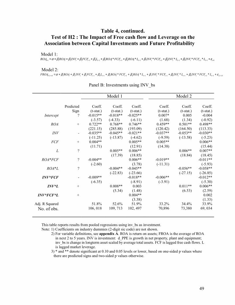
49

Table 4, continued. Test of H2 : The Impact of Free cash flow and Leverage on the

Association between Capital Investments and Future Profitability

Model 1: 1119181716151413211 ****** +−−−−−−−−+ ++++++++++= ttttttttttttttttt LFCFINVLINVFCFINVLROAFCFROALFCFINVROAROA εβββββββββα

Model 2:

521191817161514132152 ****** ttttttttttttttttttt LFCFINVLINVFCFINVLROAFCFROALFCFINVROAFROA −−−−−−−−−−+ ++++++++++= εβββββββββα

Panel B: Investments using INV_bs

Model 1 Model 2 Predicted

Sign Coeff.

(t-stat.) Coeff.

(t-stat.) Coeff.

(t-stat.) Coeff.

(t-stat.) Coeff.

(t-stat.) Coeff.

(t-stat.) Intercept ? -0.015** -0.018** -0.025** 0.007* 0.005 -0.004

(-3.57) (-4.33) (-6.11) (1.68) (1.34) (-0.92) ROA + 0.722** 0.768** 0.746** 0.459** 0.501** 0.498**

(221.15) (285.88) (193.09) (120.42) (164.50) (113.33) INV - -0.035** -0.045** -0.021** -0.037** -0.053** -0.030**

(-11.25) (-13.87) (-4.62) (-9.59) (-13.58) (-5.23) FCF + 0.004** 0.005** 0.005** 0.006**

(11.71) (12.91) (14.38) (15.44) L ? 0.005** 0.006** 0.006** 0.007**

(17.39) (18.85) (18.84) (18.45) ROA*FCF ? -0.004** 0.006** -0.019** -0.011**

(-2.60) (3.78) (-11.31) (-5.93) ROA*L ? -0.004** -0.045** -0.056** -0.058**

(-22.83) (-23.66) (-27.15) (-26.85) INV*FCF - -0.009** -0.018** -0.006** -0.012**

(-6.35) (-8.91) (-3.91) (-5.30) INV*L + 0.008** 0.003 0.011** 0.006**

(5.34) (1.48) (6.53) (2.59) INV*FCF*L + 0.004** 0.002

(3.38) (1.33) Adj. R Squared 51.8% 52.6% 51.9% 33.2% 34.4% 33.9%

No. of obs. 106, 018 109, 713 102, 497 70,896 73,380 69, 034

This table reports results from pooled regressions using inv_bs as investment. Note: 1) Coefficients on industry dummies (2-digit sic code) are not shown. 2) For variable definitions, see appendix A. ROA is return on assets; FROA is the average of ROA

in next 2 to 5 years. INV is investment: d_PPE is growth in net property, plant and equipment; inv_bs is change in longterm asset scaled by average total assets. FCF is lagged free cash flows. L is lagged market leverage.

3) * and ** denote significant at 0.10 and 0.05 levels or lower, based on one-sided p values where there are predicted signs and two-sided p values otherwise.

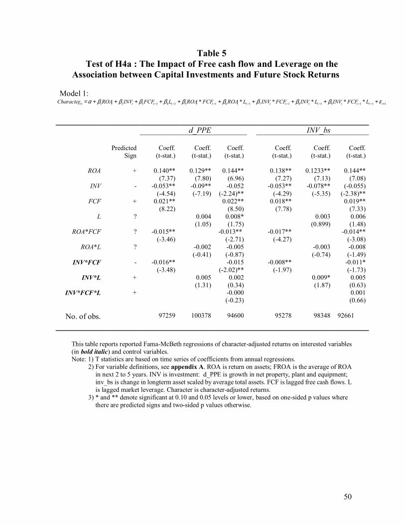
50

Table 5 Test of H4a : The Impact of Free cash flow and Leverage on the

Association between Capital Investments and Future Stock Returns Model 1:

1119181716151413211 ****** +−−−−−−−−+ ++++++++++= ttttttttttttttttt LFCFINVLINVFCFINVLROAFCFROALFCFINVROACharacter εβββββββββα

d_PPE INV_bs Predicted

Sign Coeff.

(t-stat.) Coeff.

(t-stat.) Coeff.

(t-stat.) Coeff.

(t-stat.) Coeff.

(t-stat.) Coeff.

(t-stat.)

ROA + 0.140** 0.129** 0.144** 0.138** 0.1233** 0.144** (7.37) (7.80) (6.96) (7.27) (7.13) (7.08)

INV - -0.053** -0.09** -0.052 -0.053** -0.078** (-0.055) (-4.54) (-7.19) (-2.24)** (-4.29) (-5.35) (-2.38)**

FCF + 0.021** 0.022** 0.018** 0.019** (8.22) (8.50) (7.78) (7.33)

L ? 0.004 0.008* 0.003 0.006 (1.05) (1.75) (0.899) (1.48)

ROA*FCF ? -0.015** -0.013** -0.017** -0.014** (-3.46) (-2.71) (-4.27) (-3.08)

ROA*L ? -0.002 -0.005 -0.003 -0.008 (-0.41) (-0.87) (-0.74) (-1.49)

INV*FCF - -0.016** -0.015 -0.008** -0.011* (-3.48) (-2.02)** (-1.97) (-1.73)

INV*L + 0.005 0.002 0.009* 0.005 (1.31) (0.34) (1.87) (0.63)

INV*FCF*L + -0.000 0.001 (-0.23) (0.66)

No. of obs. 97259 100378 94600 95278 98348 92661

This table reports reported Fama-McBeth regressions of character-adjusted returns on interested variables (in bold italic) and control variables. Note: 1) T statistics are based on time series of coefficients from annual regressions. 2) For variable definitions, see appendix A. ROA is return on assets; FROA is the average of ROA

in next 2 to 5 years. INV is investment: d_PPE is growth in net property, plant and equipment; inv_bs is change in longterm asset scaled by average total assets. FCF is lagged free cash flows. L is lagged market leverage. Character is character-adjusted returns.

3) * and ** denote significant at 0.10 and 0.05 levels or lower, based on one-sided p values where there are predicted signs and two-sided p values otherwise.

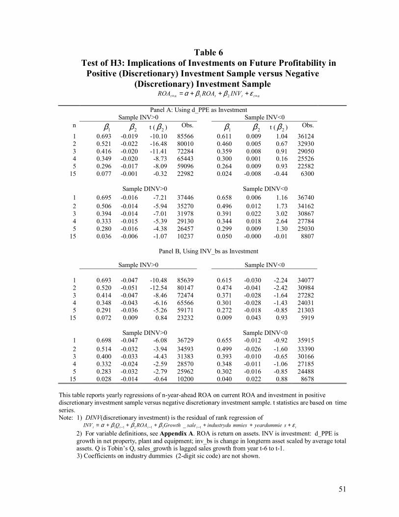
51

Table 6 Test of H3: Implications of Investments on Future Profitability in

Positive (Discretionary) Investment Sample versus Negative (Discretionary) Investment Sample

ntttnt INVROAROA ++ +++= εββα 21

Panel B, Using INV_bs as Investment

This table reports yearly regressions of n-year-ahead ROA on current ROA and investment in positive discretionary investment sample versus negative discretionary investment sample. t statistics are based on time series. Note: 1) DINV(discretionary investment) is the residual of rank regression of

ttttt syeardummiemmiesindustrydusaleGrowthROAQINV εβββα ++++++= −−− 131211 _ 2) For variable definitions, see Appendix A. ROA is return on assets. INV is investment: d_PPE is growth in net property, plant and equipment; inv_bs is change in longterm asset scaled by average total assets. Q is Tobin’s Q, sales_growth is lagged sales growth from year t-6 to t-1.

3) Coefficients on industry dummies (2-digit sic code) are not shown.

Panel A: Using d_PPE as Investment Sample INV>0 Sample INV<0

n 1β 2β t ( 2β ) Obs.

1β 2β t ( 2β ) Obs.

1 0.693 -0.019 -10.10 85566 0.611 0.009 1.04 36124 2 0.521 -0.022 -16.48 80010 0.460 0.005 0.67 32930 3 0.416 -0.020 -11.41 72284 0.359 0.008 0.91 29050 4 0.349 -0.020 -8.73 65443 0.300 0.001 0.16 25526 5 0.296 -0.017 -8.09 59096 0.264 0.009 0.93 22582

15 0.077 -0.001 -0.32 22982 0.024 -0.008 -0.44 6300 Sample DINV>0 Sample DINV<0

1 0.695 -0.016 -7.21 37446 0.658 0.006 1.16 36740 2 0.506 -0.014 -5.94 35270 0.496 0.012 1.73 34162 3 0.394 -0.014 -7.01 31978 0.391 0.022 3.02 30867 4 0.333 -0.015 -5.39 29130 0.344 0.018 2.64 27784 5 0.280 -0.016 -4.38 26457 0.299 0.009 1.30 25030

15 0.036 -0.006 -1.07 10237 0.050 -0.000 -0.01 8807

Sample INV>0 Sample INV<0

1 0.693 -0.047 -10.48 85639 0.615 -0.030 -2.24 34077 2 0.520 -0.051 -12.54 80147 0.474 -0.041 -2.42 30984 3 0.414 -0.047 -8.46 72474 0.371 -0.028 -1.64 27282 4 0.348 -0.043 -6.16 65566 0.301 -0.028 -1.43 24031 5 0.291 -0.036 -5.26 59171 0.272 -0.018 -0.85 21303

15 0.072 0.009 0.84 23232 0.009 0.043 0.93 5919 Sample DINV>0 Sample DINV<0

1 0.698 -0.047 -6.08 36729 0.655 -0.012 -0.92 35915 2 0.514 -0.032 -3.94 34593 0.499 -0.026 -1.60 33390 3 0.400 -0.033 -4.43 31383 0.393 -0.010 -0.65 30166 4 0.332 -0.024 -2.59 28570 0.348 -0.011 -1.06 27185 5 0.283 -0.032 -2.79 25962 0.302 -0.016 -0.85 24488

15 0.028 -0.014 -0.64 10200 0.040 0.022 0.88 8678

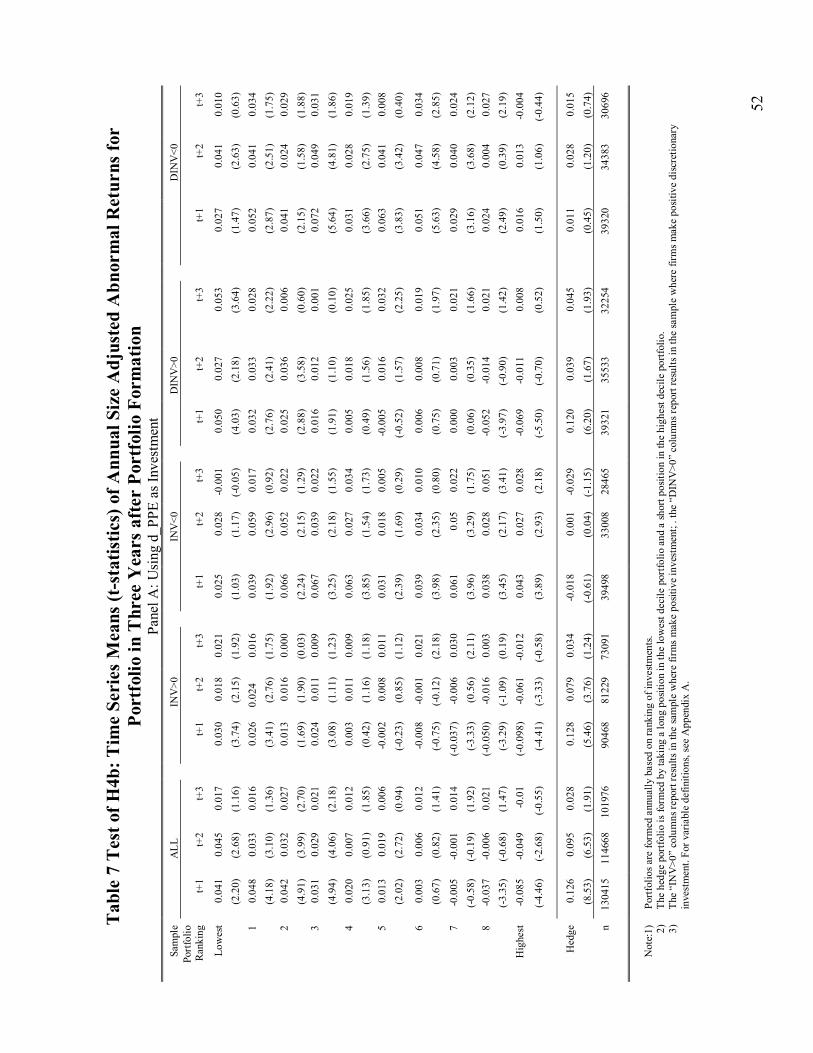
52

Tab

le 7

Tes

t of H

4b: T

ime

Seri

es M

eans

(t-s

tatis

tics)

of A

nnua

l Siz

e A

djus

ted

Abn

orm

al R

etur

ns fo

r Po

rtfo

lio in

Thr

ee Y

ears

aft

er P

ortf

olio

For

mat

ion

Pane

l A: U

sing

d_P

PE a

s Inv

estm

ent

Sam

ple

ALL

IN

V>0

INV

<0

D

INV

>0

D

INV

<0

Po

rtfo

lio

Ran

king

t+

1 t+

2 t+

3

t+1

t+2

t+3

t+

1 t+

2 t+

3

t+1

t+2

t+3

t+

1 t+

2 t+

3

Low

est

0.04

1 0.

045

0.01

7

0.03

0 0.

018

0.02

1

0.02

5 0.

028

-0.0

01

0.

050

0.02

7 0.

053

0.

027

0.04

1 0.

010

(2

.20)

(2

.68)

(1

.16)

(3.7

4)

(2.1

5)

(1.9

2)

(1

.03)

(1

.17)

(-0

.05)

(4.0

3)

(2.1

8)

(3.6

4)

(1

.47)

(2

.63)

(0

.63)

1

0.04

8 0.

033

0.01

6

0.02

6 0.

024

0.01

6

0.03

9 0.

059

0.01

7

0.03

2 0.

033

0.02

8

0.05

2 0.

041

0.03

4

(4.1

8)

(3.1

0)

(1.3

6)

(3

.41)

(2

.76)

(1

.75)

(1.9

2)

(2.9

6)

(0.9

2)

(2

.76)

(2

.41)

(2

.22)

(2.8

7)

(2.5

1)

(1.7

5)

2 0.

042

0.03

2 0.

027

0.

013

0.01

6 0.

000

0.

066

0.05

2 0.

022

0.

025

0.03

6 0.

006

0.

041

0.02

4 0.

029

(4

.91)

(3

.99)

(2

.70)

(1.6

9)

(1.9

0)

(0.0

3)

(2

.24)

(2

.15)

(1

.29)

(2.8

8)

(3.5

8)

(0.6

0)

(2

.15)

(1

.58)

(1

.88)

3

0.03

1 0.

029

0.02

1

0.02

4 0.

011

0.00

9

0.06

7 0.

039

0.02

2

0.01

6 0.

012

0.00

1

0.07

2 0.

049

0.03

1

(4.9

4)

(4.0

6)

(2.1

8)

(3

.08)

(1

.11)

(1

.23)

(3.2

5)

(2.1

8)

(1.5

5)

(1

.91)

(1

.10)

(0

.10)

(5.6

4)

(4.8

1)

(1.8

6)

4 0.

020

0.00

7 0.

012

0.

003

0.01

1 0.

009

0.

063

0.02

7 0.

034

0.

005

0.01

8 0.

025

0.

031

0.02

8 0.

019

(3

.13)

(0

.91)

(1

.85)

(0.4

2)

(1.1

6)

(1.1

8)

(3

.85)

(1

.54)

(1

.73)

(0.4

9)

(1.5

6)

(1.8

5)

(3

.66)

(2

.75)

(1

.39)

5

0.01

3 0.

019

0.00

6

-0.0

02

0.00

8 0.

011

0.

031

0.01

8 0.

005

-0

.005

0.

016

0.03

2

0.06

3 0.

041

0.00

8

(2.0

2)

(2.7

2)

(0.9

4)

(-0

.23)

(0

.85)

(1

.12)

(2.3

9)

(1.6

9)

(0.2

9)

(-0

.52)

(1

.57)

(2

.25)

(3.8

3)

(3.4

2)

(0.4

0)

6 0.

003

0.00

6 0.

012

-0

.008

-0

.001

0.

021

0.

039

0.03

4 0.

010

0.

006

0.00

8 0.

019

0.

051

0.04

7 0.

034

(0

.67)

(0

.82)

(1

.41)

(-0.7

5)

(-0.1

2)

(2.1

8)

(3

.98)

(2

.35)

(0

.80)

(0.7

5)

(0.7

1)

(1.9

7)

(5

.63)

(4

.58)

(2

.85)

7 -0

.005

-0

.001

0.

014

(-0

.037

) -0

.006

0.

030

0.

061

0.05

0.

022

0.

000

0.00

3 0.

021

0.

029

0.04

0 0.

024

(-0

.58)

(-0

.19)

(1

.92)

(-3.3

3)

(0.5

6)

(2.1

1)

(3

.96)

(3

.29)

(1

.75)

(0.0

6)

(0.3

5)

(1.6

6)

(3

.16)

(3

.68)

(2

.12)

8

-0.0

37

-0.0

06

0.02

1

(-0.0

50)

-0.0

16

0.00

3

0.03

8 0.

028

0.05

1

-0.0

52

-0.0

14

0.02

1

0.02

4 0.

004

0.02

7

(-3.3

5)

(-0.6

8)

(1.4

7)

(-3

.29)

(-1

.09)

(0

.19)

(3.4

5)

(2.1

7)

(3.4

1)

(-3

.97)

(-0

.90)

(1

.42)

(2.4

9)

(0.3

9)

(2.1

9)

Hig

hest

-0

.085

-0

.049

-0

.01

(-0

.098

) -0

.061

-0

.012

0.04

3 0.

027

0.02

8

-0.0

69

-0.0

11

0.00

8

0.01

6 0.

013

-0.0

04

(-4

.46)

(-2

.68)

(-0

.55)

(-4.4

1)

(-3.3

3)

(-0.5

8)

(3

.89)

(2

.93)

(2

.18)

(-5.5

0)

(-0.7

0)

(0.5

2)

(1

.50)

(1

.06)

(-0

.44)

Hed

ge

0.12

6 0.

095

0.02

8

0.12

8 0.

079

0.03

4

-0.0

18

0.00

1 -0

.029

0.12

0 0.

039

0.04

5

0.01

1 0.

028

0.01

5

(8.5

3)

(6.5

3)

(1.9

1)

(5

.46)

(3

.76)

(1

.24)

(-0.6

1)

(0.0

4)

(-1.1

5)

(6

.20)

(1

.67)

(1

.93)

(0.4

5)

(1.2

0)

(0.7

4)

n 13

0415

11

4668

10

1976

9046

8 81

229

7309

1

3949

8 33

008

2846

5

3932

1 35

533

3225

4

3932

0 34

383

3069

6

N

ote:

1)

Po

rtfol

ios a

re fo

rmed

ann

ually

bas

ed o

n ra

nkin

g of

inve

stm

ents

.

2)

The

hedg

e po

rtfo

lio is

form

ed b

y ta

king

a lo

ng p

ositi

on in

the

low

est d

ecile

por

tfolio

and

a sh

ort p

ositi

on in

the

high

est d

ecile

por

tfolio

. 3)

Th

e “I

NV

>0”

colu

mns

repo

rt re

sults

in th

e sa

mpl

e w

here

firm

s m

ake

posit

ive

inve

stm

ent;

. the

“D

INV

>0”

colu

mns

repo

rt re

sults

in th

e sa

mpl

e w

here

firm

s mak

e po

sitiv

e di

scre

tiona

ry

inve

stm

ent.

For v

aria

ble

defin

ition

s, se

e A

ppen

dix

A.

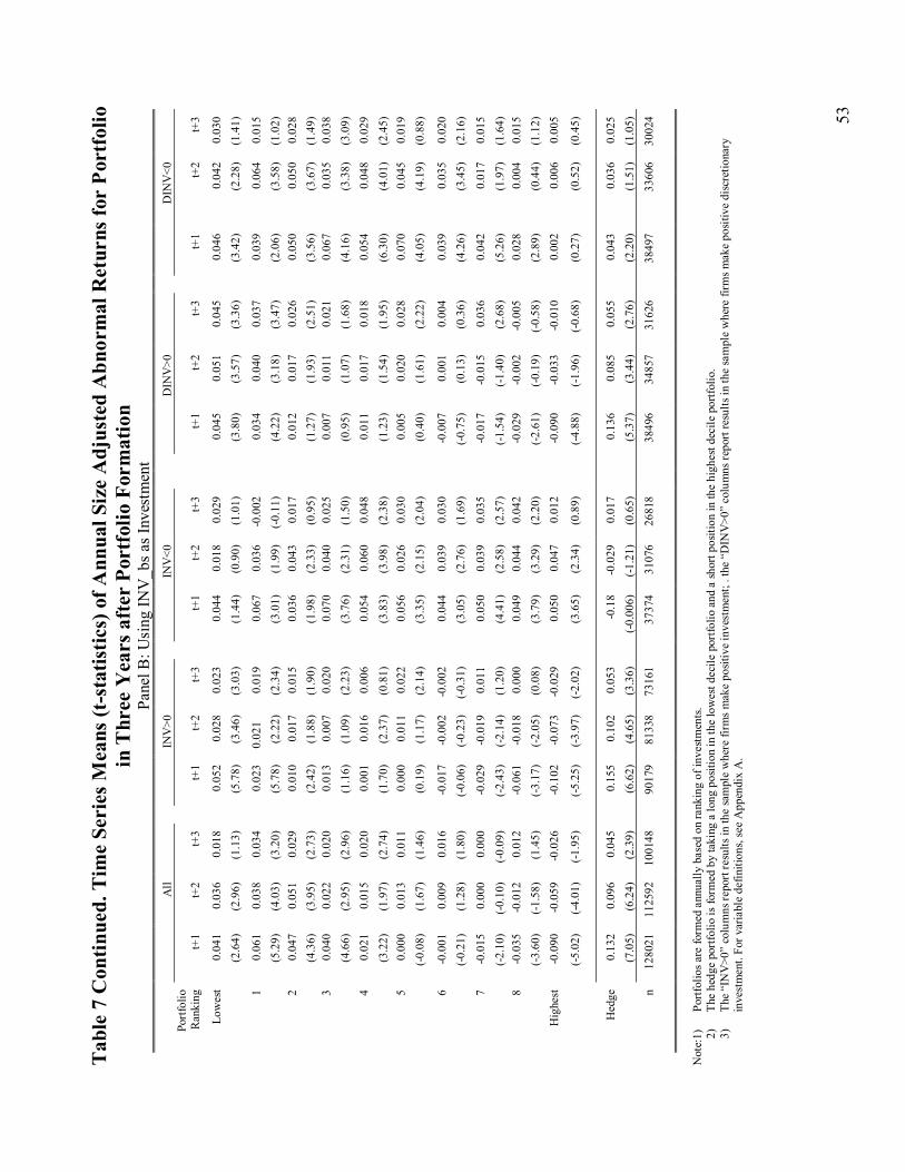
53

Tab

le 7

Con

tinue

d. T

ime

Seri

es M

eans

(t-s

tatis

tics)

of A

nnua

l Siz

e A

djus

ted

Abn

orm

al R

etur

ns fo

r Po

rtfo

lio

in T

hree

Yea

rs a

fter

Por

tfol

io F

orm

atio

n Pa

nel B

: Usi

ng IN

V_b

s as I

nves

tmen

t

A

ll

INV

>0

IN

V<0

D

INV

>0

D

INV

<0

Po

rtfo

lio

Ran

king

t+

1 t+

2 t+

3

t+1

t+2

t+3

t+

1 t+

2 t+

3

t+

1 t+

2 t+

3

t+1

t+2

t+3

Low

est

0.04

1 0.

036

0.01

8

0.05

2 0.

028

0.02

3

0.04

4 0.

018

0.02

9

0.

045

0.05

1 0.

045

0.

046

0.04

2 0.

030

(2

.64)

(2

.96)

(1

.13)

(5.7

8)

(3.4

6)

(3.0

3)

(1

.44)

(0

.90)

(1

.01)

(3

.80)

(3

.57)

(3

.36)

(3.4

2)

(2.2

8)

(1.4

1)

1 0.

061

0.03

8 0.

034

0.

023

0.02

1 0.

019

0.

067

0.03

6 -0

.002

0.

034

0.04

0 0.

037

0.

039

0.06

4 0.

015

(5

.29)

(4

.03)

(3

.20)

(5.7

8)

(2.2

2)

(2.3

4)

(3

.01)

(1

.99)

(-0

.11)

(4

.22)

(3

.18)

(3

.47)

(2.0

6)

(3.5

8)

(1.0

2)

2 0.

047

0.05

1 0.

029

0.

010

0.01

7 0.

015

0.

036

0.04

3 0.

017

0.01

2 0.

017

0.02

6

0.05

0 0.

050

0.02

8

(4.3

6)

(3.9

5)

(2.7

3)

(2

.42)

(1

.88)

(1

.90)

(1.9

8)

(2.3

3)

(0.9

5)

(1.2

7)

(1.9

3)

(2.5

1)

(3

.56)

(3

.67)

(1

.49)

3

0.04

0 0.

022

0.02

0

0.01

3 0.

007

0.02

0

0.07

0 0.

040

0.02

5

0.

007

0.01

1 0.

021

0.

067

0.03

5 0.

038

(4

.66)

(2

.95)

(2

.96)

(1.1

6)

(1.0

9)

(2.2

3)

(3

.76)

(2

.31)

(1

.50)

(0

.95)

(1

.07)

(1

.68)

(4.1

6)

(3.3

8)

(3.0

9)

4 0.

021

0.01

5 0.

020

0.

001

0.01

6 0.

006

0.

054

0.06

0 0.

048

0.01

1 0.

017

0.01

8

0.05

4 0.

048

0.02

9

(3.2

2)

(1.9

7)

(2.7

4)

(1

.70)

(2

.37)

(0

.81)

(3.8

3)

(3.9

8)

(2.3

8)

(1.2

3)

(1.5

4)

(1.9

5)

(6

.30)

(4

.01)

(2

.45)

5

0.00

0 0.

013

0.01

1

0.00

0 0.

011

0.02

2

0.05

6 0.

026

0.03

0

0.

005

0.02

0 0.

028

0.

070

0.04

5 0.

019

(-0

.08)

(1

.67)

(1

.46)

(0.1

9)

(1.1

7)

(2.1

4)

(3

.35)

(2

.15)

(2

.04)

(0

.40)

(1

.61)

(2

.22)

(4.0

5)

(4.1

9)

(0.8

8)

6 -0

.001

0.

009

0.01

6

-0.0

17

-0.0

02

-0.0

02

0.

044

0.03

9 0.

030

-0.0

07

0.00

1 0.

004

0.

039

0.03

5 0.

020

(-0

.21)

(1

.28)

(1

.80)

(-0.0

6)

(-0.2

3)

(-0.3

1)

(3

.05)

(2

.76)

(1

.69)

(-0

.75)

(0

.13)

(0

.36)

(4.2

6)

(3.4

5)

(2.1

6)

7 -0

.015

0.

000

0.00

0

-0.0

29

-0.0

19

0.01

1

0.05

0 0.

039

0.03

5

-0

.017

-0

.015

0.

036

0.

042

0.01

7 0.

015

(-2

.10)

(-0

.10)

(-0

.09)

(-2.4

3)

(-2.1

4)

(1.2

0)

(4

.41)

(2

.58)

(2

.57)

(-1

.54)

(-1

.40)

(2

.68)

(5.2

6)

(1.9

7)

(1.6

4)

8 -0

.035

-0

.012

0.

012

-0

.061

-0

.018

0.

000

0.

049

0.04

4 0.

042

-0.0

29

-0.0

02

-0.0

05

0.

028

0.00

4 0.

015

(-3

.60)

(-1

.58)

(1

.45)

(-3.1

7)

(-2.0

5)

(0.0

8)

(3

.79)

(3

.29)

(2

.20)

(-2

.61)

(-0

.19)

(-0

.58)

(2.8

9)

(0.4

4)

(1.1

2)

Hig

hest

-0

.090

-0

.059

-0

.026

-0.1

02

-0.0

73

-0.0

29

0.

050

0.04

7 0.

012

-0.0

90

-0.0

33

-0.0

10

0.

002

0.00

6 0.

005

(-5

.02)

(-4

.01)

(-1

.95)

(-5.2

5)

(-3.9

7)

(-2.0

2)

(3

.65)

(2

.34)

(0

.89)

(-4

.88)

(-1

.96)

(-0

.68)

(0.2

7)

(0.5

2)

(0.4

5)

Hed

ge

0.13

2 0.

096

0.04

5

0.15

5 0.

102

0.05

3

-0.1

8 -0

.029

0.

017

0.13

6 0.

085

0.05

5

0.04

3 0.

036

0.02

5

(7.0

5)

(6.2

4)

(2.3

9)

(6

.62)

(4

.65)

(3

.36)

(-0.0

06)

(-1.2

1)

(0.6

5)

(5.3

7)

(3.4

4)

(2.7

6)

(2

.20)

(1

.51)

(1

.05)

n 12

8021

11

2592

10

0148

9017

9 81

338

7316

1

3737

4 31

076

2681

8

38

496

3485

7 31

626

38

497

3360

6 30

024

N

ote:

1)

Po

rtfol

ios a

re fo

rmed

ann

ually

bas

ed o

n ra

nkin

g of

inve

stm

ents

.

2)

The

hedg

e po

rtfo

lio is

form

ed b

y ta

king

a lo

ng p

ositi

on in

the

low

est d

ecile

por

tfolio

and

a sh

ort p

ositi

on in

the

high

est d

ecile

por

tfolio

. 3)

Th

e “I

NV

>0”

colu

mns

repo

rt re

sults

in th

e sa

mpl

e w

here

firm

s m

ake

posit

ive

inve

stm

ent;

. the

“D

INV

>0”

colu

mns

repo

rt re

sults

in th

e sa

mpl

e w

here

firm

s mak

e po

sitiv

e di

scre

tiona

ry

inve

stm

ent.

For v

aria

ble

defin

ition

s, se

e A

ppen

dix

A.

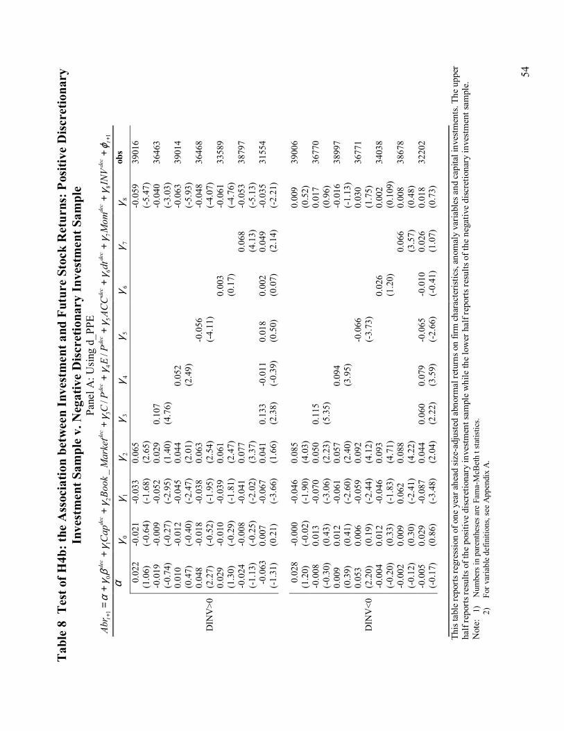
54

Tab

le 8

Tes

t of H

4b: t

he A

ssoc

iatio

n be

twee

n In

vest

men

t and

Fut

ure

Stoc

k R

etur

ns: P

ositi

ve D

iscr

etio

nary

In

vest

men

t Sam

ple

v. N

egat

ive

Dis

cret

iona

ry In

vest

men

t Sam

ple

Pane

l A: U

sing

d_P

PE

18

76

54

32

10

1/

/_

++

++

++

++

++

++

=t

dec

dec

dec

dec

dec

dec

dec

dec

dec

tIN

VM

omdt

ACC

PE

PC

Mar

ket

Book

Cap

Abr

ϕγ

γγ

γγ

γγ

γβ

γα

α

0γ

1γ

2γ

3γ

4γ

5γ

6γ

7γ

8γ

obs

0.

022

-0.0

21

-0.0

33

0.06

5

-0.0

59

3901

6

(1.0

6)

(-0.

64)

(-1.

68)

(2.6

5)

(-

5.47

)

-0

.019

-0

.009

-0

.052

0.

029

0.10

7

-0

.040

36

463

(-

0.74

) (-

0.27

) (-

2.95

) (1

.40)

(4

.76)

(-

3.03

)

0.

010

-0.0

12

-0.0

45

0.04

4

0.05

2

-0.0

63

3901

4

(0.4

7)

(-0.

40)

(-2.

47)

(2.0

1)

(2

.49)

(-5.

93)

0.04

8 -0

.018

-0

.038

0.

063

-0.0

56

-0.0

48

3646

8 D

INV

>0

(2.2

7)

(-0.

52)

(-1.

95)

(2.5

4)

(-4.

11)

(-4.

07)

0.02

9 -0

.010

-0

.039

0.

061

0.

003

-0

.061

33

589

(1

.30)

(-

0.29

) (-

1.81

) (2

.47)

(0.1

7)

(-

4.76

)

-0

.024

-0

.008

-0

.041

0.

077

0.06

8 -0

.053

38

797

(-

1.13

) (-

0.25

) (-

2.02

) (3

.37)

(4

.13)

(-

5.13

)

-0

.063

0.

007

-0.0

67

0.04

1 0.

133

-0.0

11

0.01

8 0.

002

0.04

9 -0

.035

31

554

(-

1.31

) (0

.21)

(-

3.66

) (1

.66)

(2

.38)

(-

0.39

) (0

.50)

(0

.07)

(2

.14)

(-

2.21

)

0.

028

-0.0

00

-0.0

46

0.08

5

0.00

9 39

006

(1

.20)

(-

0.02

) (-

1.90

) (4

.03)

(0.5

2)

-0.0

08

0.01

3 -0

.070

0.

050

0.11

5

0.

017

3677

0

(-0.

30)

(0.4

3)

(-3.

06)

(2.2

3)

(5.3

5)

(0.9

6)

0.00

9 0.

012

-0.0

61

0.05

7

0.09

4

-0.0

16

3899

7

(0.3

9)

(0.4

1)

(-2.

60)

(2.4

0)

(3

.95)

(-1.

13)

0.05

3 0.

006

-0.0

59

0.09

2

-0

.066

0.

030

3677

1 D

INV

<0

(2.2

0)

(0.1

9)

(-2.

44)

(4.1

2)

(-3.

73)

(1.7

5)

-0.0

04

0.01

2 -0

.046

0.

093

0.

026

0.

002

3403

8

(-0.

20)

(0.3

3)

(-1.

83)

(4.7

1)

(1

.20)

(0.1

09)

-0.0

02

0.00

9 0.

062

0.08

8

0.

066

0.00

8 38

678

(-

0.12

) (0

.30)

(-

2.41

) (4

.22)

(3

.57)

(0

.48)

-0

.005

0.

029

-0.0

87

0.04

4 0.

060

0.07

9 -0

.065

-0

.010

0.

026

0.01

8 32

202

(-

0.17

) (0

.86)

(-

3.48

) (2

.04)

(2

.22)

(3

.59)

(-

2.66

) (-

0.41

) (1

.07)

(0

.73)

Th

is ta

ble

repo

rts re

gres

sion

of o

ne y

ear a

head

size

-adj

uste

d ab

norm

al re

turn

s on

firm

char

acte

ristic

s, an

omal

y va

riabl

es a

nd c

apita

l inv

estm

ents

. The

upp

er

half

repo

rts re

sults

of t

he p

ositi

ve d

iscr

etio

nary

inve

stm

ent s

ampl

e w

hile

the

low

er h

alf r

epor

ts re

sults

of t

he n

egat

ive

disc

retio

nary

inve

stm

ent s

ampl

e.

N

ote:

1)

N

umbe

rs in

par

enth

eses

are

Fam

a-M

cBet

h t s

tatis

tics.

2)

Fo

r var

iabl

e de

finiti

ons,

see

App

endi

x A

.

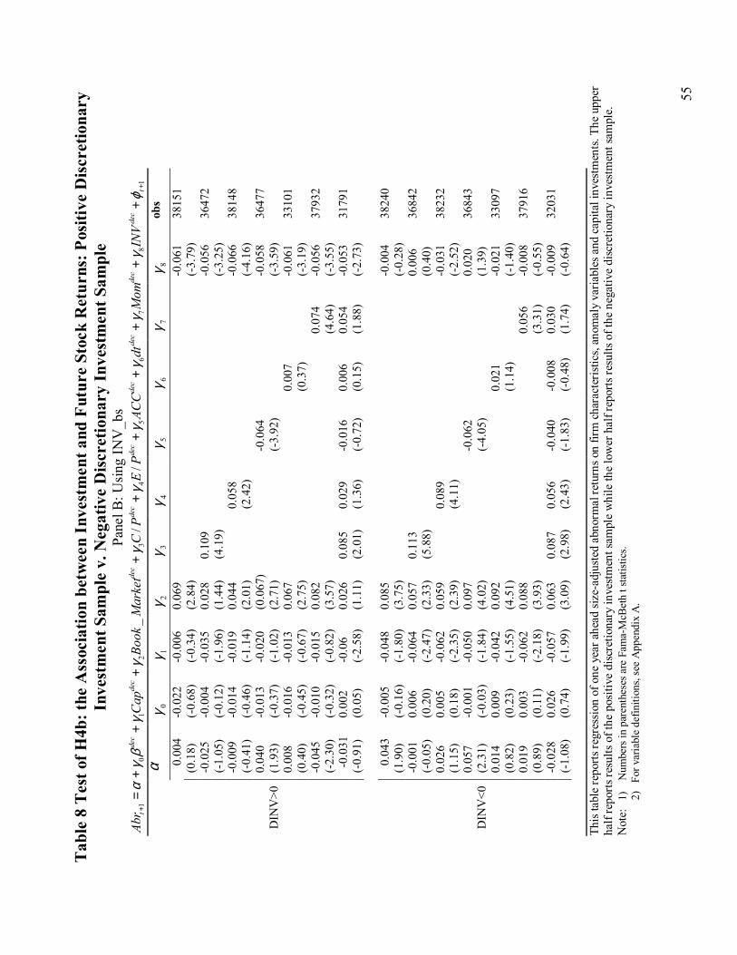
55

Tab

le 8

Tes

t of H

4b: t

he A

ssoc

iatio

n be

twee

n In

vest

men

t and

Fut

ure

Stoc

k R

etur

ns: P

ositi

ve D

iscr

etio

nary

In

vest

men

t Sam

ple

v. N

egat

ive

Dis

cret

iona

ry In

vest

men

t Sam

ple

Pane

l B: U

sing

INV

_bs

18

76

54

32

10

1/

/_

++

++

++

++

++

++

=t

dec

dec

dec

dec

dec

dec

dec

dec

dec

tIN

VM

omdt

ACC

PE

PC

Mar

ket

Book

Cap

Abr

ϕγ

γγ

γγ

γγ

γβ

γα

α

0γ

1γ

2γ

3γ

4γ

5γ

6γ

7γ

8γ

obs

0.

004

-0.0

22

-0.0

06

0.06

9

-0.0

61

3815

1

(0.1

8)

(-0.

68)

(-0.

34)

(2.8

4)

(-

3.79

)

-0

.025

-0

.004

-0

.035

0.

028

0.10

9

-0

.056

36

472

(-

1.05

) (-

0.12

) (-

1.96

) (1

.44)

(4

.19)

(-

3.25

)

-0

.009

-0

.014

-0

.019

0.

044

0.

058

-0

.066

38

148

(-

0.41

) (-

0.46

) (-

1.14

) (2

.01)

(2.4

2)

(-

4.16

)

0.

040

-0.0

13

-0.0

20

(0.0

67)

-0.0

64

-0.0

58

3647

7 D

INV

>0

(1.9

3)

(-0.

37)

(-1.

02)

(2.7

1)

(-3.

92)

(-3.

59)

0.00

8 -0

.016

-0

.013

0.

067

0.

007

-0

.061

33

101

(0

.40)

(-

0.45

) (-

0.67

) (2

.75)

(0.3

7)

(-

3.19

)

-0

.045

-0

.010

-0

.015

0.

082

0.07

4 -0

.056

37

932

(-

2.30

) (-

0.32

) (-

0.82

) (3

.57)

(4

.64)

(-

3.55

)

-0

.031

0.

002

-0.0

6 0.

026

0.08

5 0.

029

-0.0

16

0.00

6 0.

054

-0.0

53

3179

1

(-0.

91)

(0.0

5)

(-2.

58)

(1.1

1)

(2.0

1)

(1.3

6)

(-0.

72)

(0.1

5)

(1.8

8)

(-2.

73)

0.04

3 -0

.005

-0

.048

0.

085

-0

.004

38

240

(1

.90)

(-

0.16

) (-

1.80

) (3

.75)

(-0.

28)

-0.0

01

0.00

6 -0

.064

0.

057

0.11

3

0.

006

3684

2

(-0.

05)

(0.2

0)

(-2.

47)

(2.3

3)

(5.8

8)

(0.4

0)

0.02

6 0.

005

-0.0

62

0.05

9

0.08

9

-0.0

31

3823

2

(1.1

5)

(0.1

8)

(-2.

35)

(2.3

9)

(4

.11)

(-2.

52)

0.05

7 -0

.001

-0

.050

0.

097

-0.0

62

0.02

0 36

843

DIN

V<0

(2

.31)

(-

0.03

) (-

1.84

) (4

.02)

(-

4.05

)

(1

.39)

0.

014

0.00

9 -0

.042

0.

092

0.

021

-0

.021

33

097

(0

.82)

(0

.23)

(-

1.55

) (4

.51)

(1.1

4)

(-

1.40

)

0.

019

0.00

3 -0

.062

0.

088

0.05

6 -0

.008

37

916

(0

.89)

(0

.11)

(-

2.18

) (3

.93)

(3

.31)

(-

0.55

)

-0

.028

0.

026

-0.0

57

0.06

3 0.

087

0.05

6 -0

.040

-0

.008

0.

030

-0.0

09

3203

1

(-1.

08)

(0.7

4)

(-1.

99)

(3.0

9)

(2.9

8)

(2.4

3)

(-1.

83)

(-0.

48)

(1.7

4)

(-0.

64)

This

tabl

e re

ports

regr

essi

on o

f one

yea

r ahe

ad si

ze-a

djus

ted

abno

rmal

retu

rns o

n fir

m ch

arac

teris

tics,

anom

aly

varia

bles

and

cap

ital i

nves

tmen

ts. T

he u

pper

ha

lf re

ports

resu

lts o

f the

pos

itive

dis

cret

iona

ry in

vest

men

t sam

ple

whi

le th

e lo

wer

hal

f rep

orts

resu

lts o

f the

neg

ativ

e di

scre

tiona

ry in

vest

men

t sam

ple.

Not

e:

1)

Num

bers

in p

aren

thes

es a

re F

ama-

McB

eth

t sta

tistic

s.

2)

For

var

iabl

e de

finiti

ons,

see

App

endi

x A

.