University of Alberta
The Impact of Multiphase Behaviour on Coke Deposition in Heavy Oil Hydroprocessing Catalysts
by
Xiaohui Zhang
A thesis submitted to the Faculty of Graduate Studies and Research in partial fulfillment of the requirements for the degree of Doctor of Philosophy
in
Chemical Engineering
Department of Chemical and Materials Engineering
Edmonton, Alberta
Fall 2006
Abstract Coke deposition in heavy oil catalytic hydroprocessing remains a serious problem. The
influence of multiphase behaviour on coke deposition is an important but unresolved
question. A model heavy oil system (Athabasca vacuum bottoms (ABVB) + decane) and
a commercial heavy oil hydrotreating catalyst (NiMo/γ-Al2O3) were employed to study
the impact of multiphase behaviour on coke deposition.
The model heavy oil mixture exhibits low-density liquid + vapour (L1V), high-density
liquid + vapour (L2V), as well as low-density liquid + high-density liquid + vapour
(L1L2V) phase behaviour at a typical hydroprocessing temperature (380°C). The L2
phase only arises for the ABVB composition range from 10 to 50 wt %. The phase
behaviour undergoes transitions from V to L2V, to L1L2V, to L1V with increasing
ABVB compositions at the pressure examined. The addition of hydrogen into the model
heavy oil mixtures at a fixed mass ratio (0.0057:1) does not change the phase behaviour
significantly, but shifts the phase regions and boundaries vertically from low pressure to
high pressure.
In the absence of hydrogen, the carbon content, surface area and pore volume losses for
catalyst exposed to the L1 phase are greater than for the corresponding L2 phase despite a
higher coke precursor concentration in L2 than in L1. By contrast, in the presence of
hydrogen, the carbon content, surface area and pore volume losses for the catalyst
exposed to the L2 phase are greater than for the corresponding L1 phase. The higher
hydrogen concentration in L1 appears to reverse the observed results. In the presence of
hydrogen, L2 was most closely associated with coke deposition, L1 less associated with
coke deposition, and V least associated with coke deposition. Coke deposition is
maximized in the phase regions where the L2 phase arises. This key result is inconsistent
with expectation and coke deposition models where the extent of coke deposition, at
otherwise fixed reaction conditions, is asserted to be proportional to the nominal
concentration of coke precursor present in the feed.
These new findings are very significant both with respect to providing guidance
concerning possible operation improvement for existing processes and for the
development of new upgrading processes.

Acknowledgements This project would not have been a success without the unselfish contribution and help of
many people. Professor John M. Shaw gave me insightful supervision and endless
encouragement and support throughout the entire project. Not only is he a fantastic
supervisor, but also a good friend in my whole life. Professors Murray R. Gray and Alan
E. Nelson gave me most constructive criticism and valuable suggestions, which made this
project successful and shining. “Thank you” is far from what I want to say to them.
I would like to thank Drs. Yadollah Maham and Richard McFarlane for their willingness
to spend time on polishing and revising my presentations and thesis. Thanks also go to
Bei Zhao, Jessie Smith, Martin Chodakowski and Xiangyang Zou for their contribution to
this project.
I would like to thank all colleagues in the Petroleum Thermodynamics and Bitumen
Upgrading group and all support staff in the Department of Chemical and Materials
Engineering. Without your help and cooperation, this undertaking would not have been
possible.
I gratefully acknowledge the Scholarship programs at the University of Alberta and
research funds from the sponsors of the NSERC Industrial Research Chair in Petroleum
Thermodynamics (Alberta Energy Research Institute, Albian Sands Energy Inc.,
Computer Modelling Group Ltd., ConocoPhillips Inc., Imperial Oil Resources, NEXEN
Inc., Natural Resources Canada, Petroleum Society of the CIMM, Oilphase-DBR,
Oilphase – a Schlumberger Company, Schlumberger, Syncrude Canada Ltd., NSERC).
No words could describe my debt to my parents and my siblings for their sacrifices and
for giving me the opportunity to pursue higher education. My success is attributed to their
incessant encouragement and support.
Special thanks to my life’s partner, Chongguo, for her love, her sacrifice, her
encouragement, ……, to make one of the most important steps in my life successful.
Table of Contents 1. INTRODUCTION........................................................................................... 1
1.1 Background..............................................................................................................................................1
1.2 Coke Deposition Phenomena..................................................................................................................2
1.2.1 Coke Deposition Models on Catalyst ................................................................................................2
1.2.2 Coke Deposition along Catalyst Beds in Trickle-Bed Reactors ........................................................3
1.2.3 Coke Suppression by Addition of Solvents .......................................................................................4
1.3 What Can Be Learned from Carbon Rejection Processes? .................................................................4
1.4 Preceding Work.......................................................................................................................................5
1.5 Hypothesis ................................................................................................................................................6
1.6 Objectives.................................................................................................................................................8
1.7 Thesis Outline ..........................................................................................................................................9
2. LITERATURE REVIEW............................................................................... 10
2.1 Heavy Oils ..............................................................................................................................................10
2.1.1 Heavy Oils/Bitumen-Our Future Energy Resource .........................................................................10
2.1.2 Characteristics of Heavy Oils/bitumen ............................................................................................11
2.1.3 Asphaltenes......................................................................................................................................12
2.2 Heavy Oil Catalytic Hydroprocessing .................................................................................................15
2.2.1 Introduction .....................................................................................................................................15
2.2.2 Fixed-Bed Processes........................................................................................................................17
2.2.3 Moving-Bed Processes ....................................................................................................................19
2.2.4 Ebullated-Bed Processes..................................................................................................................21
2.2.5 Slurry Phase Process........................................................................................................................24
2.2.6 Catalyst Characteristics ...................................................................................................................25
2.3 Catalyst Coking .....................................................................................................................................27
2.3.1 Catalyst Fouling Mechanisms..........................................................................................................27
2.3.2 Fouling by Coke ..............................................................................................................................27
2.3.3 Coke Formation Chemistry..............................................................................................................29
2.3.4 Coke Deposition Modes ..................................................................................................................31
2.3.5 Coke Formation Kinetics.................................................................................................................32
2.3.6 Minimisation of Catalyst Fouling....................................................................................................35
2.4 The Role of Phase Behaviour in Coke Formation ..............................................................................37
2.4.1 Introduction .....................................................................................................................................37
2.4.2 Some Basic Theories of Phase Behaviour .......................................................................................37
2.4.3 The Role of Phase Behaviour in Thermal Cracking ........................................................................48
2.4.4 The Role of Phase Behaviour in Hydroprocessing ..........................................................................51
2.4.5 Coke Formation Mechanism Involving Colloidal Phenomena........................................................54
2.5 Summary................................................................................................................................................55
3. EXPERIMENTAL ........................................................................................ 56
3.1 Materials ................................................................................................................................................56
3.2 X-ray View Cell .....................................................................................................................................58
3.2.1 Experimental Set-up ........................................................................................................................58
3.2.2 Working Principles ..........................................................................................................................59
3.2.3 Illustration of a Single X-ray Transmission Image..........................................................................62
3.2.4 Flow Diagram..................................................................................................................................63
3.3 The Selection of Model Fluid System...................................................................................................65
3.4 Phase Behaviour Experiments..............................................................................................................65
3.5 Catalyst Presulfidation..........................................................................................................................66
3.6 Catalyst Coking Experiments...............................................................................................................67
3.7 Catalyst Characterization.....................................................................................................................70
4. PHASE BEHAVIOUR OF ABVB + DECANE MIXTURES.......................... 72
4.1 Introduction ...........................................................................................................................................72
4.2 Pressure-Temperature and Pressure-Composition Phase Diagrams................................................72
4.2.1 P-T Phase Diagram..........................................................................................................................72
4.2.2 P-x Phase Diagram ..........................................................................................................................80
4.3 Evolution of P-x Phase Diagrams with Temperature.........................................................................81
5. PHASE BEHAVIOUR OF ABVB + DECANE + HYDROGEN MIXTURES . 85
5.1 Introduction ...........................................................................................................................................85
5.2 The Impact of Hydrogen on the Phase Behaviour of ABVB + Decane mixtures.............................85
6. THE IMPACT OF MULTIPHASE BEHAVIOUR ON COKE DEPOSITION IN CATALYSTS EXPOSED TO ABVB + DECANE MIXTURES ............................ 89
6.1 Introduction ...........................................................................................................................................89
6.2 Catalyst Coking Experimental Design.................................................................................................89
6.3 Bulk Properties of the Coked Catalyst Pellets. ...................................................................................90
6.4 Characteristics of Cross Sections of Coked Catalyst Pellets..............................................................94
6.5 Possible Explanations for Greater Deposition in Catalysts Exposed to L1 vs L2............................98
6.6 Origin of the Bimodal Pore Size Distribution. ..................................................................................100
6.7 Summary..............................................................................................................................................100
7. THE IMPACT OF MULTIPHASE BEHAVIOUR ON COKE DEPOSITION IN CATALYST EXPOSED TO ABVB + DECANE + HYDROGEN MIXTURES.... 102
7.1 Introduction .........................................................................................................................................102
7.2 Catalyst Coking Experimental Design...............................................................................................102
7.3 The Impact of Hydrogen Addition on Coke Deposition...................................................................103
7.4 The Impact of Pressure on Coke Deposition.....................................................................................106
7.5 The Effect of Composition on Coke Deposition ................................................................................107
7.6 Summary..............................................................................................................................................108
8. COKE DEPOSITION MODELS................................................................. 113
8.1 Coke Deposition Variation with Comparison ...................................................................................113
8.2 Thoughts on Coke Deposition Models ...............................................................................................114
8.3 Summary..............................................................................................................................................115
9. PROCESS IMPLICATIONS ...................................................................... 116
9.1 Introduction .........................................................................................................................................116
9.2 Trickle-Bed Reactor ............................................................................................................................116
9.3 Solvent Addition Processes and Supercritical Hydrogenation Processes .......................................117
9.4 Summary..............................................................................................................................................118
10. CONCLUSIONS .................................................................................... 119
REFERENCES................................................................................................. 122
APPENDIX I. GENERAL EXPERIMENTAL PROCEDURE USING X-RAY VIEW CELL ................................................................................................................ 133
APPENDIX II. X-RAY TRANSMISSION IMAGES 137
APPENDIX III. PHASE EQUILIBRIUM RAW DATA.................................... 15050
APPENDIX IV. SKETCH OF A VARIABLE CATALYST HOLDER ................. 160
APPENDIX V. SUMMARY OF CATALYST COKING EXPERIMENTS AND THEIR REPEATABILITY ................................................................................. 161
List of Tables Table 3.1 Physical and chemical properties of ABVB (Zou, 2003) ................... 56
Table 3.2 Chemicals used and their purity, suppliers. ...................................... 57
Table 6.1 Elemental analysis of coked catalysts .............................................. 91
Table 6.2 BET analysis of coked catalysts ....................................................... 92
Table 7.1 The impact of hydrogen addition on coke deposition...................... 104
Table 7.2 Experimental conditions for experiments associated with Table 7.1
.................................................................................................................. 105
Table 7.3 Experimental conditions for the experiments associated with Figure
7.5. ............................................................................................................ 109
List of Figures Figure 1.1 Schematic representation of coke deposition models........................ 3
Figure 1.2 Coke profiles along catalyst bed depth. a) Amemiya et al., 2000; b)
Niu, 2001 ....................................................................................................... 4
Figure 1.3 Hypothesized ternary phase diagram during hydroprocessing.......... 7
Figure 2.1 Petroleum fractionation.................................................................... 12
Figure 2.2 Average structure of Athabasca asphaltene molecules. a)
pericondensed model (Zhao et al. 2001); b) archipelago model (Sheremata
et al. 2004). ................................................................................................. 13
Figure 2.3 Proposed mechanism for asphaltene conversion: a) destruction of
asphaltene micelle; b) depolymerization due to heteroatom removal (Asaoka
et al. 1983; Takeuchi et al. 1983) ................................................................ 14
Figure 2.4 Share of the various residue hydroprocessing technologies in
upgrading of atmospheric and vacuum residues, respectively. ................... 16
Figure 2.5 Schematic of fixed-bed reactor........................................................ 17
Figure 2.6 The Gulf resid hydrodesulfurization process. .................................. 18
Figure 2.7 Schematic of bunker reactor............................................................ 20
Figure 2.8 Process flow scheme of the HYCON unit. ....................................... 21
Figure 2.9 Schematic of LC-Fining reactor ....................................................... 22
Figure 2.10 The H-Oil process.......................................................................... 23
Figure 2.11 The CANMET process................................................................... 25
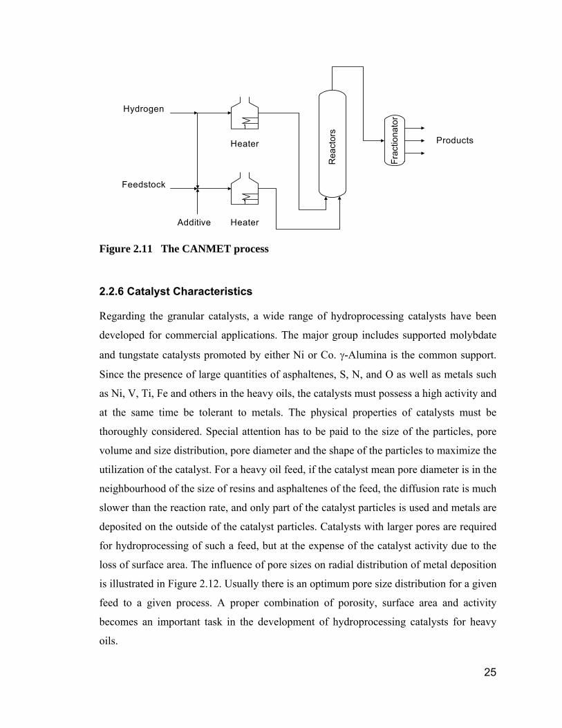
Figure 2.12 Radial distribution of metals on catalyst pellets ............................. 26
Figure 2.13 Schematic representation of position-dependent foulant deposition
profiles. a) coke and b) metals. ................................................................... 26
Figure 2.14 Catalyst fouling profiles ................................................................. 28
Figure 2.15 Coke formation pathway................................................................ 32
Figure 2.16 A) Schematic representation of position–dependent coke deposition
profiles in catalyst beds batch or continuous; B) radial distribution of coke
within a single pellet; a) parallel and b) series. ............................................ 35
Figure 2.17 Phase behaviours exhibited by hydrocarbon mixtures. Dashed
phase boundaries indicate critically identical phases. ................................. 38
Figure 2.18 Phase behaviour classification for binary mixtures ........................ 41
Figure 2.19 Schematic Type V phase behaviour for a binary system. a: PTx
three-dimensions; b: PT and Tx projections of the PTx three-dimensions .. 42
Figure 2.20 Expansion of P-T diagrams of Type V phase behaviour from binary
mixtures to ternary mixtures ........................................................................ 44
Figure 2.21 P-x phase diagram of a solvent (CO2) + crude oil system (Pollack
and Enick, 1988) ......................................................................................... 46
Figure 2.22 Ternary phase behaviour of the asphalt-oil-propane mixture at a
temperature close to the critical temperature of propane (Wilson, Keith and
Haylett, 1936 ). ............................................................................................ 47
Figure 2.23 Generalized phase diagram at constant temperature and pressure
for reservoir fluids, and heavy oil and bitumen + diluent mixtures. .............. 48
Figure 2.24 Schematic representation of coke formation ................................. 49
Figure 2.25 Partial phase diagram for the model heavy oil ABVB 25 wt % +
dodecane 73 wt % + hydrogen 2 wt %. ....................................................... 52
Figure 2.26 Residuum Hydrocracking Reaction Mechanism ............................ 53
Figure 3.1 Pore size distribution of catalyst ...................................................... 57
Figure 3.2 Isotherms of catalyst........................................................................ 58
Figure 3.3 Schematics of X-ray view cell .......................................................... 59
Figure 3.4 Schematic of X-ray absorption ........................................................ 61
Figure 3.5 Illustration using a single X-ray transmission image........................ 63
Figure 3.6 Intensity and density profile corresponding to the single X-ray image
in Figure 3.5 ................................................................................................ 64
Figure 3.7 View cell flow diagram..................................................................... 64
Figure 3.8 X-ray transmission images and schematic representations for: a)
showing catalyst held in the L1 and L2 phases of a mixture; and b) showing
catalyst held in the L1 phase with the L2 phase dispersed. ........................ 68
Figure 3.9 Temperature profile for catalyst coking experiments. ...................... 69
Figure 4.1 X-ray images of ABVB (10 wt %) + decane mixture. ....................... 74
Figure 4.2 P-T phase diagram of 10% ABVB + decane mixture....................... 75
Figure 4.3 P-T phase diagram of 20% ABVB + decane mixture....................... 75
Figure 4.4 P-T phase diagram of 25% ABVB + decane mixture....................... 76
Figure 4.5 P-T phase diagram of 30% ABVB + decane mixture....................... 76
Figure 4.6 P-T phase diagram of 35% ABVB + decane mixture....................... 77
Figure 4.7 P-T phase diagram of 40% ABVB + decane mixture....................... 77
Figure 4.8 P-T phase diagram of 50% ABVB + decane mixture....................... 78
Figure 4.9 P-T phase diagram of 70% ABVB + decane mixture....................... 78
Figure 4.10 P-T phase diagram of 90% ABVB + decane mixture..................... 79
Figure 4.11 P-T phase diagram of 100% ABVB + decane mixture................... 79
Figure 4.12 X-ray images of 10% to 100% ABVB + decane mixtures at 380 °C
.................................................................................................................... 82
Figure 4.13 P-x phase diagram at 380 °C ........................................................ 82
Figure 4.14 P-x phase diagram at 320 °C ........................................................ 83
Figure 4.15 Sketches of P-x phase diagrams evolution for ABVB+decane
mixtures at three characteristic temperatures. a) T < decane critical
temperature; b) T just greater than decane critical temperature; c) T > the
temperature at which the left hand L1V zone collapses into the LLV zone. 84
Figure 5.1 P-T phase diagram of 10% ABVB + decane + hydrogen mixture.... 86
Figure 5.2 P-T phase diagram of 20% ABVB + decane + hydrogen mixture.... 86
Figure 5.3 P-T phase diagram of 30% ABVB + decane + hydrogen mixture.... 87
Figure 5.4 P-T phase diagram of 40% ABVB + decane + hydrogen mixture.... 87
Figure 5.5 P-x phase diagram at 380 °C .......................................................... 88
Figure 6.1 Phase behaviour for catalyst coking experiments with the mixture 30
wt% ABVB + decane. .................................................................................. 90
Figure 6.2 Pore size distributions of coked catalysts for 2 hrs of coking........... 93
Figure 6.3 Pore size distributions of coked catalysts for 5 hrs of coking........... 93
Figure 6.4 Adsorption/desorption isotherms of coked catalyst following 2 hrs of
coking. ......................................................................................................... 94
Figure 6.5 Adsorption/desorption isotherms of coked catalyst following 5 hrs of
coking.......................................................................................................... 94
Figure 6.6 Element distributions within catalyst pellets for a) carbon (including
carbon coating), b) vanadium, c) sulphur for 5 hours of coked catalyst and d)
for the carbon coating on fresh catalyst....................................................... 96
Figure 6.7 Photomicrographs of catalyst cross-sections for a) fresh catalyst; b)
2hr coked catalyst in L1; c) 2hr coked catalyst in L2; d) 5hr coked catalyst in
L1+ L2 dispersed; e) 5hr coked catalyst in L1; f) 5hr coked catalyst in L2. . 97
Figure 6.8 Modified bulk phase coke deposition model .................................... 97
Figure 6.9 Asphaltene aggregate size distribution for a) ABVB (32 wt %
asphaltenes); b) 5% ABVB in dodecane (1.6 % asphaltenes). (Zhang et al.
2005) ........................................................................................................... 99
Figure 6.10 A comparison of (a) the pore size distribution and (b) sorption
isotherm for powdered and pellet coked catalyst samples from the 5 hr, L1 +
L2 dispersed case. .................................................................................... 100
Figure 7.1 The conditions for the catalyst coking experiments with ABVB +
decane + hydrogen. The hydrogen to feed mass ratio was fixed at 0.0057.
.................................................................................................................. 103
Figure 7.2 Pore size distributions of fresh catalyst and coked catalyst for a
hydrogen/feed ratio of 0.0057.................................................................... 105
Figure 7.3 Adsorption/desorption isotherms of fresh catalyst and coked catalyst
for a hydrogen/feed ratio of 0.0057. .......................................................... 106
Figure 7.4 The effect of pressure on coke deposition on catalysts under the
hydrodynamic regime illustrated in Figure 3.8b. Except as noted, phase
volumes are measured ~ 15 minutes after coking reaction at 380 °C. ...... 107
Figure 7.5 The effect of phase behavior on coke deposition at 0.57 wt %
hydrogen. a) carbon content in coked catalyst; b) coked catalyst pore
volume; c) coked catalyst surface area; d) adsorption/desorption isotherms
and e) pore size distributions..................................................................... 112
Figure 8.1 Comparison of coke deposition profiles for ABVB + decane +
hydrogen mixtures which exhibit multiphase behaviour and ABVB + 1-methyl
naphthalene + hydrogen mixtures which exhibit two phase behaviour. (All
data from batch reactor) ............................................................................ 114
Figure 8.2 A sketch of comparison between the experimental coke deposition
profile involving multiphase behaviour and the predicted coke deposition
profile with simple conventional kinetics at a fixed reaction time. .............. 115
Figure 9.1 Schematics of flow pattern in trickle-bed hydroprocessing reactor. a)
a trickling flow pattern; and b) the flow pattern around a single pellet, in the
presence of two liquid phases. .................................................................. 117
List of Symbols A The light component in a binary mixture
ABVB Athabasca Bitumen Vacuum Bottoms
AR Atmospheric residue
As Surface area
A+ Reactant asphaltenes
A* Asphaltene cores
A*max Maximum asphaltene cores that can be held in solution
A*ex Excess asphaltene cores beyond what can be held in solution
B The heavy component in a binary mixture
C Concentration of coke precursor
CCR Conradson carbon reduction
CF Concentration of feed
CI Concentration of intermediate
CRS Surface reactant concentration
CSTR Continuous-stirred tank reactor
E Energy of X-ray photons, keV
F Feed
HDM Hydrodemetallization
HDN Hydrodenitrogenation
HDS Hydrodesulfurization
H+ Non-volatile heptane soluble reactant
H* Non-volatile heptane soluble product
I Intermediate
I Intensity of transmitted beam
I0 Intensity of the incidental beam
k Constant for mass adsorption coefficient
K point Point where L1 and V become critical in the presence of L2
kF Rate constant for parallel fouling
kI Rate constant for series fouling
ka Adsorption rate constant
Ka Equilibrium adsorption constant
kc Rate constant for catalytic coking
kt Rate constant for thermal coking
L point Point where L1 and L2 become critical in the presence of V
L Liquid phase
L1 Low-density liquid phase
L2 High-density liquid phase
LCEP Lower critical end point
P Pressure
PH2 Hydrogen partial pressure
q Coke amount
q0 Coke amount corresponding to complete fouling
qc Carbon amount
qc,max Maximum carbon amount
qmax Maximum estimated coke amount
R Total rate of coking
Rc Rate of catalytic coking
Rt Rate of thermal coking
SARA Saturates – Aromatics – Resins – Asphaltenes
SAXS Small Angle X-rays Scattering
T Temperature
TI Toluene-insoluble coke
UCEP Upper critical end point
V Vapour phase
V Volatiles
Vp Pore volume
VR Vacuum residue
w Cumulative feed to catalyst ratio, a pseudo time coordinate
wi Mass fraction of component i
x Composition
x Thickness
Greek Letters
εy Particle porosity
η Effectiveness factor
λ Wavelength of X-ray beam
λe Effective wavelength of polychromatic X-ray beam
μ Mass absorption coefficient
μi Mass absorption coefficient of component i for a monochromatic x-ray
beam at wavelength λ.
μij Mass absorption coefficient of component i for a polychromatic x-ray
beam at a wavelength of λj.
ρ Density
ρx Microparticle density
1
1. Introduction
1.1 Background
As the world’s supply of conventional light sweet crude oils becomes depleted, the
petroleum industry is forced to refine heavy crude oils to supply the increasing demand
for transport fuels. These heavy crudes often contain significant amounts of asphaltenes,
sulfur, nitrogen and metal-containing organic compounds that foul catalysts used in
conventional catalytic cracking and hydrocracking operations. As a consequence, an
upgrading process is required to remove most of the sulphur, nitrogen, and metals and to
convert part of the heavy ends to lighter distillates before these heavy crudes can be used
as feedstocks for existing conventional refinery processes. A number of such upgrading
processes have been developed and can be roughly classified into three types: (1) carbon
rejection, (2) hydrogen addition and (3) heteroatom removal, with or without catalysts.
Hydropocessing is one of the primary upgrading processes, which is characterized by
hydrogen addition, heteroatom removal, minimal carbon rejection, using catalysts. It is
widely used as a primary upgrading process in the petroleum industry because this
process can obtain a much higher yield and quality of liquid products compared to carbon
rejection processes. This feature may make this process more profitable especially in the
situation of continuously increasing crude and transport fuel prices and stringent
environmental requirements. But there exists a rapid loss of catalyst activity in
hydroprocessing of heavy oils due to the significant amounts of asphaltenes, sulphur,
nitrogen and metal-containing organic compounds, hence increasing production cost.
Therefore, hydroprocessing must achieve a compromise between high yields of light
hydrocarbon liquids and catalyst cost and longevity.
The fouling of catalysts still remains a major problem even though extensive studies have
been carried out to minimize coking over catalyst, including: catalyst preparation, reactor
design, operating condition optimization, processes development. Many methods have
been adopted, singly or in combination to deal with the processing problems associated
with heavy oils. All of these approaches represent compromises between product yield,
quality and catalyst cost, catalyst lifetime, and process equipment cost. And there is room
2
for considerable improvement in the technology for upgrading heavy oils and refinery
residues.
Coke formation mechanisms are a key theoretical base for guidance with respect to
minimizing coke formation and optimizing hydroprocessing. Although coke formation
mechanisms have been investigated intensively, there appear to be inconsistencies
between coking kinetics models and observed coke deposition phenomena. In addition,
some observed phenomena related to coke deposition occurring in hydroprocessing
cannot be explained satisfactorily, while others can be interpreted from several
perspectives.
1.2 Coke Deposition Phenomena
1.2.1 Coke Deposition Models on Catalyst
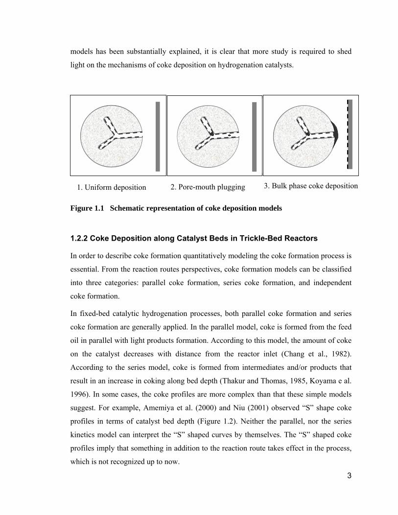
All coke deposition mechanisms on catalyst are classified into three simplified models:
uniform surface deposition (Richardson et al. 1996), pore-mouth plugging (Muegge and
Massoth, 1991), and bulk phase coke deposition (Richardson et al. 1996). The schematic
representation of coke deposition models is shown in Figure 1.1. The Uniform deposition
model assumes that coke deposits uniformly on catalyst inner surfaces. The pore-mouth
plugging model includes uniform coke deposition on inner surfaces of catalysts but also
allows for coke deposition at the small pore mouths within catalysts, leading to local pore
blockages. The bulk phase coke deposition model shows that coke will form in the liquid
phase and deposit on all surfaces within the reactors and includes both the uniform coke
deposition and pore mouth plugging. Detailed descriptions of these three coke deposition
models are presented in the literature review.
Uniform surface deposition and pore mouth plugging models are two hotly-debated
models because conflicting results were reported on the probable location of coke
deposits on hydroprocessing catalyst. Observation of bulk phase coke deposition makes
the understanding of coke deposition mechanisms more complex. All models are
supported by experimental findings; however, there are no satisfactory theories
explaining why coke deposits in three different modes. Since none of the conflicting
3
models has been substantially explained, it is clear that more study is required to shed
light on the mechanisms of coke deposition on hydrogenation catalysts.
Figure 1.1 Schematic representation of coke deposition models
1.2.2 Coke Deposition along Catalyst Beds in Trickle-Bed Reactors
In order to describe coke formation quantitatively modeling the coke formation process is
essential. From the reaction routes perspectives, coke formation models can be classified
into three categories: parallel coke formation, series coke formation, and independent
coke formation.
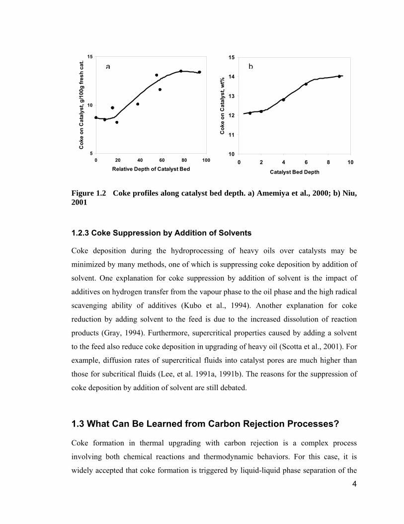
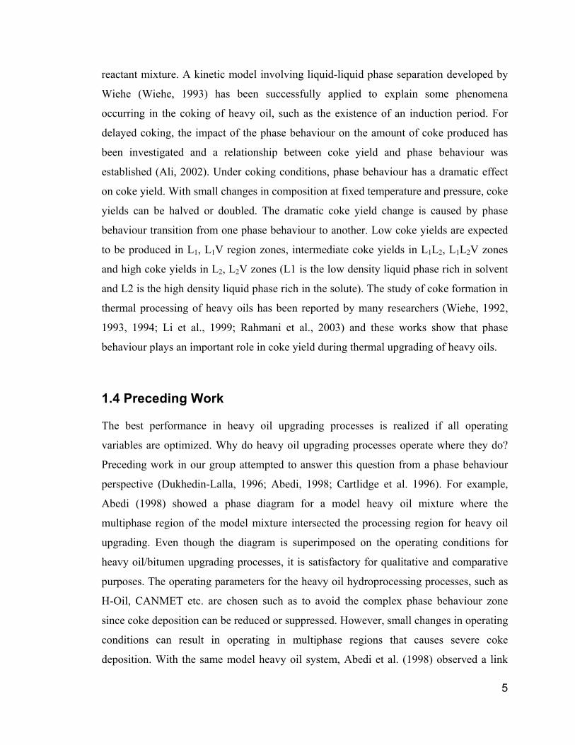
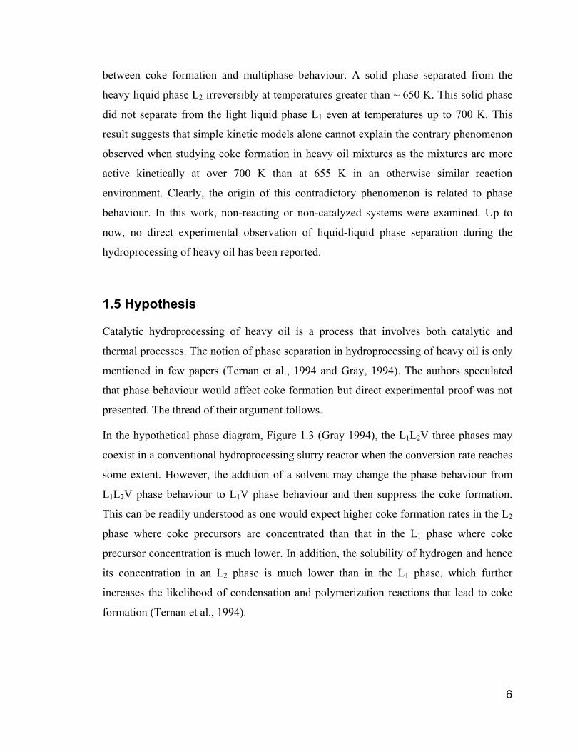
In fixed-bed catalytic hydrogenation processes, both parallel coke formation and series
coke formation are generally applied. In the parallel model, coke is formed from the feed
oil in parallel with light products formation. According to this model, the amount of coke
on the catalyst decreases with distance from the reactor inlet (Chang et al., 1982).
According to the series model, coke is formed from intermediates and/or products that
result in an increase in coking along bed depth (Thakur and Thomas, 1985, Koyama e al.
1996). In some cases, the coke profiles are more complex than that these simple models
suggest. For example, Amemiya et al. (2000) and Niu (2001) observed “S” shape coke
profiles in terms of catalyst bed depth (Figure 1.2). Neither the parallel, nor the series
kinetics model can interpret the “S” shaped curves by themselves. The “S” shaped coke
profiles imply that something in addition to the reaction route takes effect in the process,
which is not recognized up to now.
1. Uniform deposition 2. Pore-mouth plugging 3. Bulk phase coke deposition
4
Figure 1.2 Coke profiles along catalyst bed depth. a) Amemiya et al., 2000; b) Niu, 2001
1.2.3 Coke Suppression by Addition of Solvents
Coke deposition during the hydroprocessing of heavy oils over catalysts may be
minimized by many methods, one of which is suppressing coke deposition by addition of
solvent. One explanation for coke suppression by addition of solvent is the impact of
additives on hydrogen transfer from the vapour phase to the oil phase and the high radical
scavenging ability of additives (Kubo et al., 1994). Another explanation for coke
reduction by adding solvent to the feed is due to the increased dissolution of reaction
products (Gray, 1994). Furthermore, supercritical properties caused by adding a solvent
to the feed also reduce coke deposition in upgrading of heavy oil (Scotta et al., 2001). For
example, diffusion rates of supercritical fluids into catalyst pores are much higher than
those for subcritical fluids (Lee, et al. 1991a, 1991b). The reasons for the suppression of
coke deposition by addition of solvent are still debated.
1.3 What Can Be Learned from Carbon Rejection Processes?
Coke formation in thermal upgrading with carbon rejection is a complex process
involving both chemical reactions and thermodynamic behaviors. For this case, it is
widely accepted that coke formation is triggered by liquid-liquid phase separation of the
5
10
15
0 20 40 60 80 100
Relative Depth of Catalyst Bed
Cok
e on
Cat
alys
t, g/
100g
fres
h ca
t.
10
11
12
13
14
15
0 2 4 6 8 10
Catalyst Bed Depth
Cok
e on
Cat
alys
t, w
t%
a b
5
reactant mixture. A kinetic model involving liquid-liquid phase separation developed by
Wiehe (Wiehe, 1993) has been successfully applied to explain some phenomena
occurring in the coking of heavy oil, such as the existence of an induction period. For
delayed coking, the impact of the phase behaviour on the amount of coke produced has
been investigated and a relationship between coke yield and phase behaviour was
established (Ali, 2002). Under coking conditions, phase behaviour has a dramatic effect
on coke yield. With small changes in composition at fixed temperature and pressure, coke
yields can be halved or doubled. The dramatic coke yield change is caused by phase
behaviour transition from one phase behaviour to another. Low coke yields are expected
to be produced in L1, L1V region zones, intermediate coke yields in L1L2, L1L2V zones
and high coke yields in L2, L2V zones (L1 is the low density liquid phase rich in solvent
and L2 is the high density liquid phase rich in the solute). The study of coke formation in
thermal processing of heavy oils has been reported by many researchers (Wiehe, 1992,
1993, 1994; Li et al., 1999; Rahmani et al., 2003) and these works show that phase
behaviour plays an important role in coke yield during thermal upgrading of heavy oils.
1.4 Preceding Work
The best performance in heavy oil upgrading processes is realized if all operating
variables are optimized. Why do heavy oil upgrading processes operate where they do?
Preceding work in our group attempted to answer this question from a phase behaviour
perspective (Dukhedin-Lalla, 1996; Abedi, 1998; Cartlidge et al. 1996). For example,
Abedi (1998) showed a phase diagram for a model heavy oil mixture where the
multiphase region of the model mixture intersected the processing region for heavy oil
upgrading. Even though the diagram is superimposed on the operating conditions for
heavy oil/bitumen upgrading processes, it is satisfactory for qualitative and comparative
purposes. The operating parameters for the heavy oil hydroprocessing processes, such as
H-Oil, CANMET etc. are chosen such as to avoid the complex phase behaviour zone
since coke deposition can be reduced or suppressed. However, small changes in operating
conditions can result in operating in multiphase regions that causes severe coke
deposition. With the same model heavy oil system, Abedi et al. (1998) observed a link
6
between coke formation and multiphase behaviour. A solid phase separated from the
heavy liquid phase L2 irreversibly at temperatures greater than ~ 650 K. This solid phase
did not separate from the light liquid phase L1 even at temperatures up to 700 K. This
result suggests that simple kinetic models alone cannot explain the contrary phenomenon
observed when studying coke formation in heavy oil mixtures as the mixtures are more
active kinetically at over 700 K than at 655 K in an otherwise similar reaction
environment. Clearly, the origin of this contradictory phenomenon is related to phase
behaviour. In this work, non-reacting or non-catalyzed systems were examined. Up to
now, no direct experimental observation of liquid-liquid phase separation during the
hydroprocessing of heavy oil has been reported.
1.5 Hypothesis
Catalytic hydroprocessing of heavy oil is a process that involves both catalytic and
thermal processes. The notion of phase separation in hydroprocessing of heavy oil is only
mentioned in few papers (Ternan et al., 1994 and Gray, 1994). The authors speculated
that phase behaviour would affect coke formation but direct experimental proof was not
presented. The thread of their argument follows.
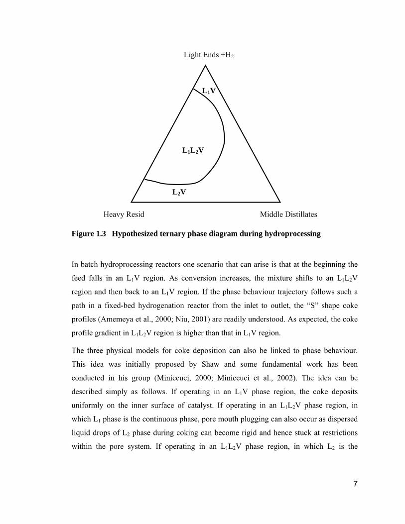
In the hypothetical phase diagram, Figure 1.3 (Gray 1994), the L1L2V three phases may
coexist in a conventional hydroprocessing slurry reactor when the conversion rate reaches
some extent. However, the addition of a solvent may change the phase behaviour from
L1L2V phase behaviour to L1V phase behaviour and then suppress the coke formation.
This can be readily understood as one would expect higher coke formation rates in the L2
phase where coke precursors are concentrated than that in the L1 phase where coke
precursor concentration is much lower. In addition, the solubility of hydrogen and hence
its concentration in an L2 phase is much lower than in the L1 phase, which further
increases the likelihood of condensation and polymerization reactions that lead to coke
formation (Ternan et al., 1994).
7
Figure 1.3 Hypothesized ternary phase diagram during hydroprocessing
In batch hydroprocessing reactors one scenario that can arise is that at the beginning the
feed falls in an L1V region. As conversion increases, the mixture shifts to an L1L2V
region and then back to an L1V region. If the phase behaviour trajectory follows such a
path in a fixed-bed hydrogenation reactor from the inlet to outlet, the “S” shape coke
profiles (Amemeya et al., 2000; Niu, 2001) are readily understood. As expected, the coke
profile gradient in L1L2V region is higher than that in L1V region.
The three physical models for coke deposition can also be linked to phase behaviour.
This idea was initially proposed by Shaw and some fundamental work has been
conducted in his group (Miniccuci, 2000; Miniccuci et al., 2002). The idea can be
described simply as follows. If operating in an L1V phase region, the coke deposits
uniformly on the inner surface of catalyst. If operating in an L1L2V phase region, in
which L1 phase is the continuous phase, pore mouth plugging can also occur as dispersed
liquid drops of L2 phase during coking can become rigid and hence stuck at restrictions
within the pore system. If operating in an L1L2V phase region, in which L2 is the
Light Ends +H2
L1L2V
L2V
L1V
Middle Distillates Heavy Resid
8
continuous phase, or in the L2V region coke can readily deposit on all surfaces present in
a reactor.
If one can prove the occurrence of phase separation in hydroprocessing of heavy oil and
that higher coke yields arise in L2V and L1L2V regions than in L1V regions, and establish
a link between the three types of phase behaviour and three coke deposition models, such
findings would provide a sound basis for upgrading process development and operation
improvement. At the same time, such findings would add an additional dimension to the
complexity of hydrogenation catalyst fouling models.
1.6 Objectives
Understanding the link between kinetics and phase behaviour is invaluable when
developing kinetic models for coke formation, developing mechanisms for coke
deposition, and designing or optimizing hydroprocessing processes. Phase behaviour can
change dramatically giving rise to very different phenomena with seemingly very little
difference in operating conditions. Knowledge of the location of “danger zones” and
operating away from them can dramatically increase the productivity and life of
expensive hydrogenation catalysts.
The principal objectives of this study are to establish a relationship between phase
behaviour and coke formation kinetics and coke deposition in hydroprocessing processes.
Applied issues include elucidation of catalyst fouling mechanisms in hydroprocessing
processes. If successful the investigation will become a touchstone for future research in
this area. The specific objectives are to:
1. Observe the phase behaviour of selected mixtures in which coke precursors exist and
identify a suitable operating condition for coke formation and deposition experiments;
2. Investigate the influence of phase behaviour on the coke deposition in different phase
regions;
3. Establish a relationship between the nature of coke deposition (coke deposition
model) and phase behaviour.
9
1.7 Thesis Outline
Following this brief introduction, a comprehensive literature review related to this thesis
is presented in Chapter 2 to help readers better understand topics addressed subsequently
e.g.: heavy oil characteristics, currently commercialized heavy oil catalytic
hydroprocessing technologies, coke deposition mechanisms and models. The
experimental equipment and procedures are described in Chapter 3. The X-ray
transmission view cell was used to explore the phase behaviour of the model heavy oil
system, which provided guidance for the catalyst coking experiments and the view cell
was also modified and used as a batch reactor for catalyst coking experiments. The coked
catalysts were characterized by traditional methods. For clarity, the experimental results
and discussions are divided into several chapters with each chapter focusing on a specific
topic. Chapter 4 and 5 focus on the phase behaviour study of the model heavy oil system
in the presence and absence of hydrogen, respectively. The direct observation of complex
phase behaviour in this model heavy oil system is provided and the phase diagrams are
constructed. Chapter 6 and 7 provide the results from the investigation of catalyst coking
in the presence and absence of hydrogen, respectively, where the impact of phase
behaviour and factors associated with phase behaviour on coke deposition are discussed.
Chapter 8 and Chapter 9 address the catalyst coking kinetics and industrial process
implication, separately. Finally, conclusions are presented in Chapter 10.
10
2. Literature Review
The origin and focus of the thesis are presented in chapter 1. In this chapter, background
materials needed to understand and appreciate the details presented in subsequent
chapters are presented. Topics addressed include:
(1) The chemical and physical characteristics of heavy oil/bitumen, especially the
troublemaking fraction, asphaltene fraction.
(2) A brief review of current catalytic hydroprocessing technologies for heavy
oil/bitumen.
(3) A general description of catalyst fouling, in particular the coke formation which is
one of the major causes of catalyst fouling.
(4) A basic introduction to phase diagram theory needed to construct phase diagrams for
the model heavy oil system used in this project.
(5) A summary of recent developments related to this project both in thermal upgrading
and catalytic hydroprocessing of heavy oil/bitumen.
2.1 Heavy Oils
2.1.1 Heavy Oils/Bitumen-Our Future Energy Resource
With the depletion of conventional crude oils, the heavy oil and bitumen resources are
increasingly becoming commercially producible, since the early 80's in the Athabasca,
Alberta, Canada and, more recently, in the Orinoco, Venezuela. For example, in Canada,
most liquid hydrocarbons are currently produced from bitumen: there is 1.7 to 2.5 trillion
barrels of bitumen (one-third of the world's known petroleum reserves) in Alberta, which
could meet Canada’s energy needs for the next two centuries (Morgan, 2001; Gray and
Masliyah, 2004).
As the world’s supply of conventional light sweet crude oils becomes depleted, the
petroleum industry is forced to refine heavy crude oils and bitumen to supply the
increasing demand for transport fuels and petrochemical feeds. Meanwhile the market for
11
heavier fuels is decreasing while that for middle distillates is increasing at a rapid rate, so
ideally heavy oils and bitumen recovered in the upstream oil fields, along with residues
produced in the downstream refineries, should be upgraded as much as possible into
middle distillates.
A key to the full realization of the upgrading potential of these heavy oil reserves and
heavy residues will be technology, and more precisely how to find methods allowing to
process theses residues at acceptable costs and without excessive energy consumption.
2.1.2 Characteristics of Heavy Oils/bitumen
Understanding of heavy oil/bitumen composition and properties is a prerequisite for
investigation of phase equilibrium and kinetics of heavy oil mixtures in upgrading
processes. Heavy oils/bitumens include atmosphere residues (AR) and vacuum residues
(VR), topped crude oils, coal oil extracts, crude oils extracted from tar sands, etc. (Gray,
1994; Speight, 2002), and in this context, are generally called as heavy oil. Heavy oil is
very viscous and does not flow easily. The characteristics of heavy oils are quite different
from those of conventional crude oils. They generally have a high specific gravity
(>0.95), a low hydrogen-to-carbon ratio (~1.5), and contain large amounts of asphaltenes
(>5 wt %), heavy metals (such as vanadium and nickel), heteroatoms (such as sulfur,
nitrogen and oxygen) and inorganic fine solids (Speight, 1991). The inorganic fine solids,
heavy metals and heteroatoms tend to concentrate in the heaviest fractions, such as resins
and asphaltenes (Reynolds, 1994 & 1999; Chung et al. 1997).
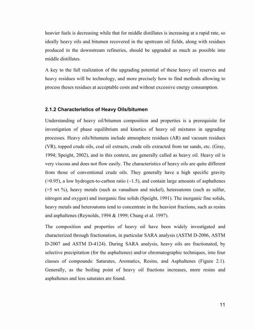
The composition and properties of heavy oil have been widely investigated and
characterized through fractionation, in particular SARA analysis (ASTM D-2006, ASTM
D-2007 and ASTM D-4124). During SARA analysis, heavy oils are fractionated, by
selective precipitation (for the asphaltenes) and/or chromatographic techniques, into four
classes of compounds: Saturates, Aromatics, Resins, and Asphaltenes (Figure 2.1).
Generally, as the boiling point of heavy oil fractions increases, more resins and
asphaltenes and less saturates are found.
12
Feed stock
Insolubles Deasphaltened Oil
Insolubles Asphaltenes Resins Aromatics Saturates
n-Heptane
Benzene or Toluene Chromatographic
Figure 2.1 Petroleum fractionation
2.1.3 Asphaltenes
Asphaltene represents the most refractory fraction of heavy oils. The importance of
asphaltene in the petroleum industry is through its negative impact on various petroleum
operations, such as exploration, production, transportation, and refining. One needs to
have a good understanding of the chemical properties and colloidal behaviour of
asphaltenes in order to avoid or resolve the problems caused by them.
Asphaltenes are identified by SARA analysis as a solubility class which may be
composed of molecules that differ significantly in their chemical characteristics (e.g.
molar mass, aromaticity, heteroatom and metal content etc.). The chemical composition
of asphaltene depends on many variables, including choice of alkane solvent, volume,
temperature, and time of mixing, as well as carbonaceous fuel source. Asphaltenes
generally have a high content of heavy metals and heteroatoms, which results in a high
coking tendency.
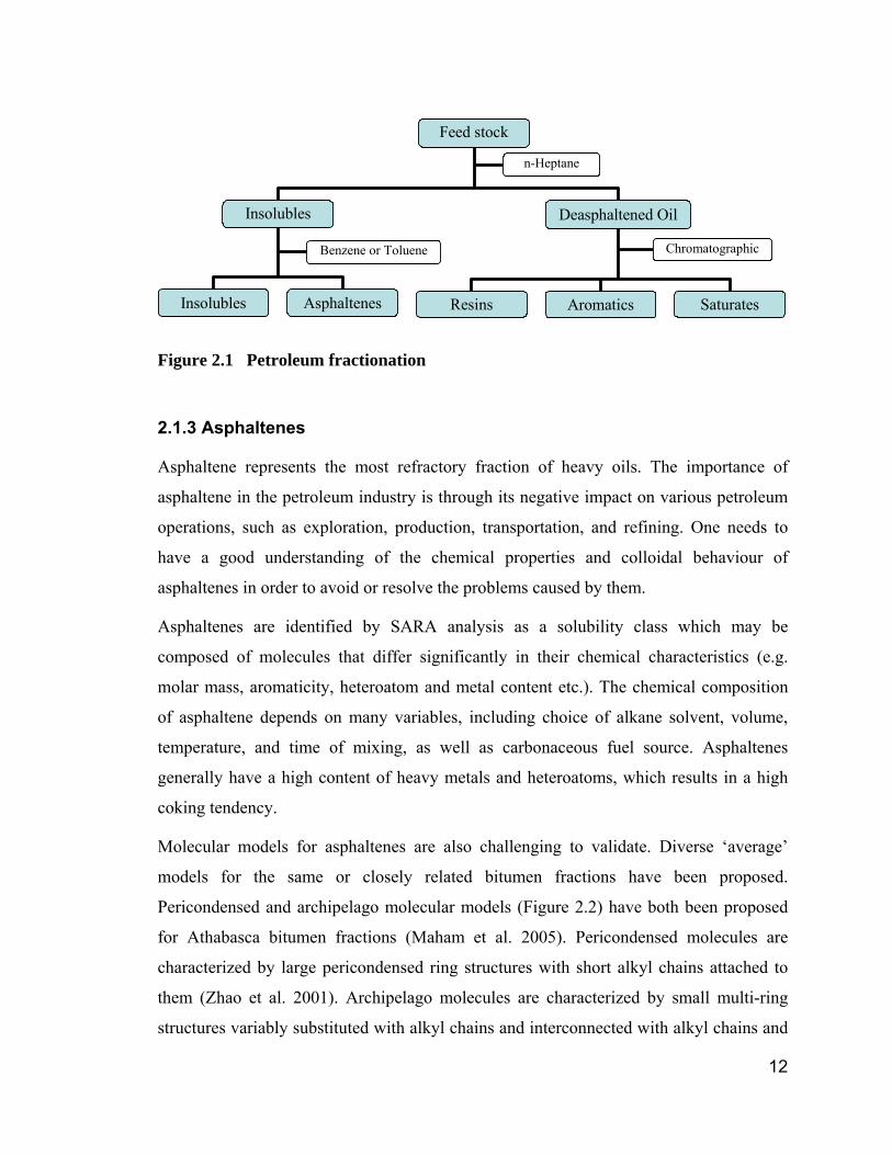
Molecular models for asphaltenes are also challenging to validate. Diverse ‘average’
models for the same or closely related bitumen fractions have been proposed.
Pericondensed and archipelago molecular models (Figure 2.2) have both been proposed
for Athabasca bitumen fractions (Maham et al. 2005). Pericondensed molecules are
characterized by large pericondensed ring structures with short alkyl chains attached to
them (Zhao et al. 2001). Archipelago molecules are characterized by small multi-ring
structures variably substituted with alkyl chains and interconnected with alkyl chains and
13
heteroatom bridges (Murgich et al. 1999; Strausz et al., 1992; Sheremata et al. 2004). The
average molecule structures proposed appear to relate to the relative importance that
researchers place on different analytical techniques.
SS
S
Figure 2.2 Average structure of Athabasca asphaltene molecules. a) pericondensed model (Zhao et al. 2001); b) archipelago model (Sheremata et al. 2004).
The physics and chemistry arising at the supramolecular level are equally unresolved,
even though great efforts have been devoted. It has been concluded that heavy oils such
as crude oils, residues, bitumen etc. exhibit colloidal behaviour in the presence of
asphaltenes, and resin fractions (Li et al. 1996; Bardon et al. 1996; Branco et al. 2001).
The asphaltenes are believed to exist in heavy oils partly dissolved and partly in steric-
colloidal and/or micellar forms depending on the polarity of their oil medium and
presence of other compounds (Priyanto et al. 2001). The asphaltene aggregates
dimensions are on the colloidal length scale. Early work showed that the size of
asphaltene particles varies between nanometer and micron length scales (Overfield et al.,
1989; Yen, 1998). The dimensions of aggregates also depend strongly on the nature of
14
the solvent, asphaltene concentration, and temperature (Espinat et al. 1998). The most
characteristic trait of asphaltenes is their strong aggregation propensity in hydrocarbon
solution (Overfield et al., 1989). Under unfavorable surrounding conditions, asphaltenes
are prone to aggregation by flocculation or micellization, and can precipitate from the oil
matrix if the colloid stability of the feed cannot be maintained (Mansoori, 1997).
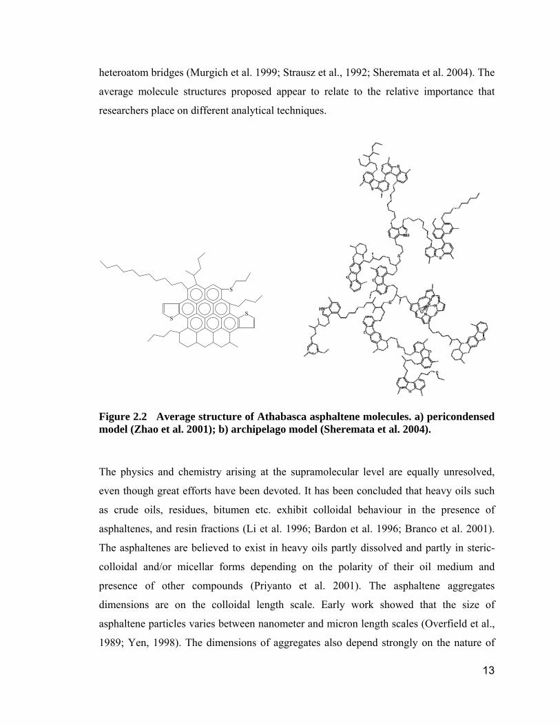
The conversion of asphaltene is a complex decomposition process (Quann et al. 1988;
Dautzenberg and De Deken, 1987). Based on the micelle macrostructures of asphaltene, a
generalized sequential asphaltene conversion mechanism was proposed by Takeuchi et al.
1983 and Asaoka et al. 1983 shown in Figure 2.3. Mechanistic studies of asphaltene
conversion indicate that metal removal (Vanadium and nickel) plays an important role at
the initial step of asphaltene conversion since the metals contained in asphaltene micelles
are the bonding constituents to form the asphaltene micelles and the removal of metals
destroys the association of asphaltene micelles. Subsequently, further dissociation occurs
from depolymerization and thermal cleavage of weak links by weakening of π bond
interactions between aromatic sheets and by removal of heteroatoms such as sulphur.
Figure 2.3 Proposed mechanism for asphaltene conversion: a) destruction of asphaltene micelle; b) depolymerization due to heteroatom removal (Asaoka et al. 1983; Takeuchi et al. 1983)
There are diverse views concerning the molecular structure and colloidal behaviour of
asphaltenes. Also since the chemistry and physics of asphaltenes are unresolved, the
conversion mechanisms of asphaltenes are uncertain. More efforts need to be devoted
Metal Aromatic sheet Aliphatic Week link
a b
15
into the study of both the microscopic and macroscopic structure and conversion
mechanisms of asphaltenes. However, there is a growing consensus one way or another
on each matter.
2.2 Heavy Oil Catalytic Hydroprocessing
2.2.1 Introduction
Process selection of upgrading technologies depends on the combination of cost, product
slate, and byproduct considerations. Since the petroleum is depleting, recently process
selection has tended to favour hydroprocessing technologies, which maximize distillate
yield and minimize byproducts (especially coke) and generally accomplish significant
demetallization and Conradson carbon reduction (CCR), in addition to desulfurization
and viscosity reduction. A spectrum of hydroprocessing technologies for heavy oils is
available, summarized in several review papers and books including comparison of
different technologies (Qabazard et al. 1990; Furimsky, 1998; Dautzenberg and De
Deken, 1984; Quann et al. 1988; Gosselink and van Veen, 1999) and a list of
technologies available (Absi-Halabi et al. 1997; Speight, 2000; Speight and Ozum, 2002;
Dukhedin-Lalla, 1996). This review here is limited to catalytic hydroprocessing
technologies used for the treatment of heavy oils and bitumen.
In summary, catalytic hydropocessing is characterized by hydrogen addition, heteroatom
removal, minimal carbon rejection, using catalysts (Le Page et al. 1992). In the presence
of a hydrogenation catalyst, the hydrogen is able to be added into feed and converts
heteroatoms to hydrogen sulphide, water, and ammonia etc. and the coke formation is
suppressed at the same time. Not only does the hydrogenation catalyst enhance
hydrogenation reactions, but it also serves as a surface for the deposition of metals.
Based on the type of reactor bed employed, commercial catalytic reactors using a
granular catalyst can be divided into the three main categories (Le Page et al. 1992;
Furimsky, 1998): (a) Fixed-bed processes; (b) Moving-bed processes; (c) Ebullated-bed
processes.
16
Traditionally, fixed-bed reactors were used for hydroprocessing of light feeds. Gradually
fixed-bed reactors were modified to accommodate heavier feeds. Many fixed-bed
reactors can operate reliably on atmospheric residues. However a good operability cannot
be achieved with difficult feeds such as vacuum residues. Major concern is the excessive
number of catalyst replacement. In contrast, the moving- and ebullated-bed units have
demonstrated reliable operations with vacuum residues.
The processes using granular catalyst involve a high cost of the hydroprocessing catalyst
caused by the catalyst replacement and disposal, so an alternative process ie. slurry-phase
process, is obtaining growing interest. This process employs disposable catalysts, which
is added to the feed as finely divided solids. The once-through catalyst will remain in the
slag.
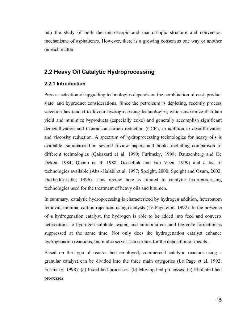
Therefore several criteria have to be considered to make choices among these options.
But the availability ensures that a wide range of feeds can be processed if an optimal
match between the reactor with the catalyst and the feed of interest is made. Figure 2.4
illustrates the relative positions of the various technologies in processing atmospheric and
vacuum residues (Scheffer et al. 1998). In the present review, each reactor system except
for the homogeneous system is discussed briefly and exemplified with typical processes
in commercial operation or near a commercial stage.
37%
47%
5%
10% 1%
88%
2%9%
fixed ebullated slurry moving homogeneous
Atmospheric residue Vacuum residue
Figure 2.4 Share of the various residue hydroprocessing technologies in upgrading of atmospheric and vacuum residues, respectively.
17
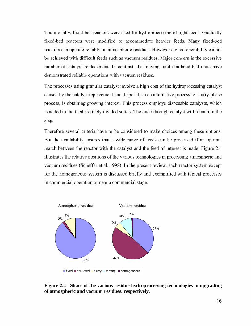
2.2.2 Fixed-Bed Processes
Fixed-bed processes are well developed and have been in commercial use for several
decades. The most typical fixed-bed reactor in hydroprocessing is the trickle-bed reactor.
The trickle-bed process is relatively easy and simple to operate and scale up. A schematic
of the fixed-bed or trickle-bed reactor is shown in Figure 2.5 (Beaton and Bertolacini,
1991). The reactor operates in a downflow mode, with liquid feed trickling downward
over the stationary solid catalyst cocurrent with the hydrogen gas. Since the
hydrogenation is an exothermal reaction, in some cases, hydrogen is introduced between
the beds as a quench to prevent excessive high temperatures within the reactor.
The main limitation of this type of reactor is the gradual accumulation of metals in the
pores of the catalyst and the final blockage of access for reactants to catalyst surface
when a typical residue is processed. After the catalyst deactivates, the reactor must be
shut down and the catalyst bed has to be replaced, which usually takes a longer time
around 10-20 days and is uneconomical.
Figure 2.5 Schematic of fixed-bed reactor
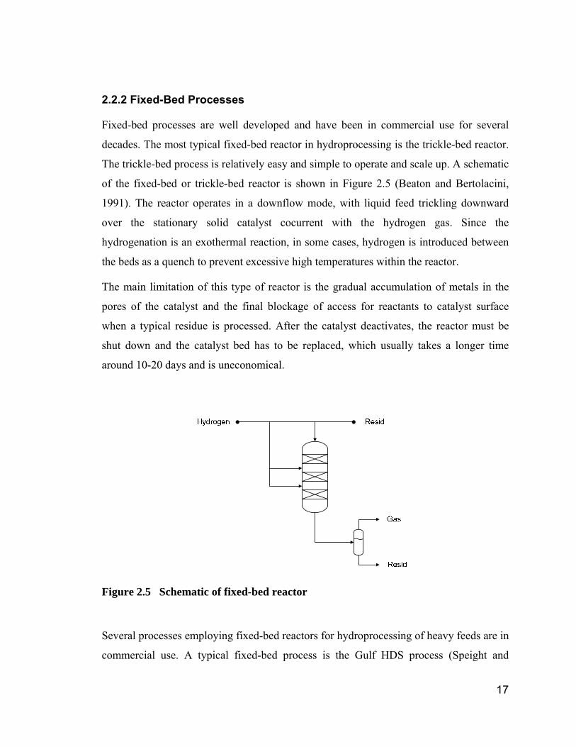
Several processes employing fixed-bed reactors for hydroprocessing of heavy feeds are in
commercial use. A typical fixed-bed process is the Gulf HDS process (Speight and
18
Ozum, 2002; Speight, 2000; Mckinney and Stipanov, 1971; Yanik et al., 1977), which
upgrades residua by catalytic hydrogenation to refined heavy fuel oils or to high quality
catalytic charge stocks. In addition, the process can be used, through alternative designs,
to upgrade high sulfur crude oils or bitumen that are unsuited for the more conventional
refining techniques. A simplified flowsheet of the Gulf resid hydrodesulfuriztion process
is shown in Figure 2.6. The feedstock is heated together with hydrogen and recycle gas
and charged to the downflow reactor. The liquid product goes to fractionation after
flashing to produce the various product streams. On-stream cycles of 4-5 months can be
obtained at desulfurization levels of 65-75%, and catalyst life may be as long as 2 years.
Make-up hydrogen Recycle hydrogen
Feedstock
Heater
Reactors
Abso
rber
Frac
tiona
tor
Vacu
um
High pressure separator
Low pressure separator
Bottoms
Bottoms
Heavy gas oil
Light gas oil
Heavy Naphtha
Gasoline
Gas revoery
Figure 2.6 The Gulf resid hydrodesulfurization process.
IFP has developed several kinds of fixed-bed processes under the name HYVAHL
(Kressmann et al. 1998; Furimsky, 1998; Speight, 2000). The HYVAHL-F process is a
classical fixed-bed process using several fixed-bed reactors in series. A recent
improvement on the HYVAHL-F process has been made, namely, a swing reactor system
is used in front of several fixed bed reactors in series, which is named as HYVAHL-S
process. This improvement enables on-stream catalyst replacement. Hydrodemetallation
is achieved in the swing reactor system and a relatively high level of conversion is
achieved at the same time. Hydrodesulfurization is achieved in the following fixed bed
19
reactors in series. With this arrangement, HDS and HDM levels of 92% and 95% for
Arabian light or Arabian heavy vacuum residues, respectively, can be achieved.
A number of other fixed-bed systems are also available in commercial use. The ABC
(asphaltenic bottom cracking), licensed by the Chiyoda Chemical Engineering &
Construction Co. Ltd., is a fixed-bed catalytic hydrotreating process coupled with a
solvent deasphalting unit (Dukhedin-Lalla, 1996; Speight, 2000). The ABC process is
suitable for hydrodemetallization, asphaltene cracking and moderate
hydrodesulfurization. The RCD (reduced crude to distillate) Unibon process (Dukhedin-
Lalla, 1996; Speight, 2000), licensed by UOP Inc., employs a series of fixed-bed reactors
to remove contaminants such as nitrogen, sulphur and heavy metals from atmospheric
residues at moderately high hydrogen pressures. The BOC (black oil conversion) process,
an extension of the RCD process, operates at higher hydrogen pressures for
hydroprocessing of vacuum residues (Dukhedin-Lalla, 1996; Speight, 2000).
2.2.3 Moving-Bed Processes
These processes are able to realize continuous catalyst renewal by utilizing moving-bed
reactors. The advantage of this moving-bed process is able to process heavy feeds,
especially rich in metals. This technology combines the advantage of fixed-bed operation
in a plug flow and the ebullated-bed operation in easy catalyst replacement. The well-
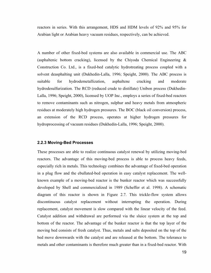
known example of a moving-bed reactor is the bunker reactor which was successfully
developed by Shell and commercialized in 1989 (Scheffer et al. 1998). A schematic
diagram of this reactor is shown in Figure 2.7. This trickle-flow system allows
discontinuous catalyst replacement without interrupting the operation. During
replacement, catalyst movement is slow compared with the linear velocity of the feed.
Catalyst addition and withdrawal are performed via the sluice system at the top and
bottom of the reactor. The advantage of the bunker reactor is that the top layer of the
moving bed consists of fresh catalyst. Thus, metals and salts deposited on the top of the
bed move downwards with the catalyst and are released at the bottom. The tolerance to
metals and other contaminants is therefore much greater than in a fixed-bed reactor. With
20
this capability, the bunker reactor system may be suitable for hydroprocessing of very
heavy feeds, especially when several reactors are combined in series.
Feed
Fresh/regenerated catalyst
Product
Spent catalyst
Figure 2.7 Schematic of bunker reactor.
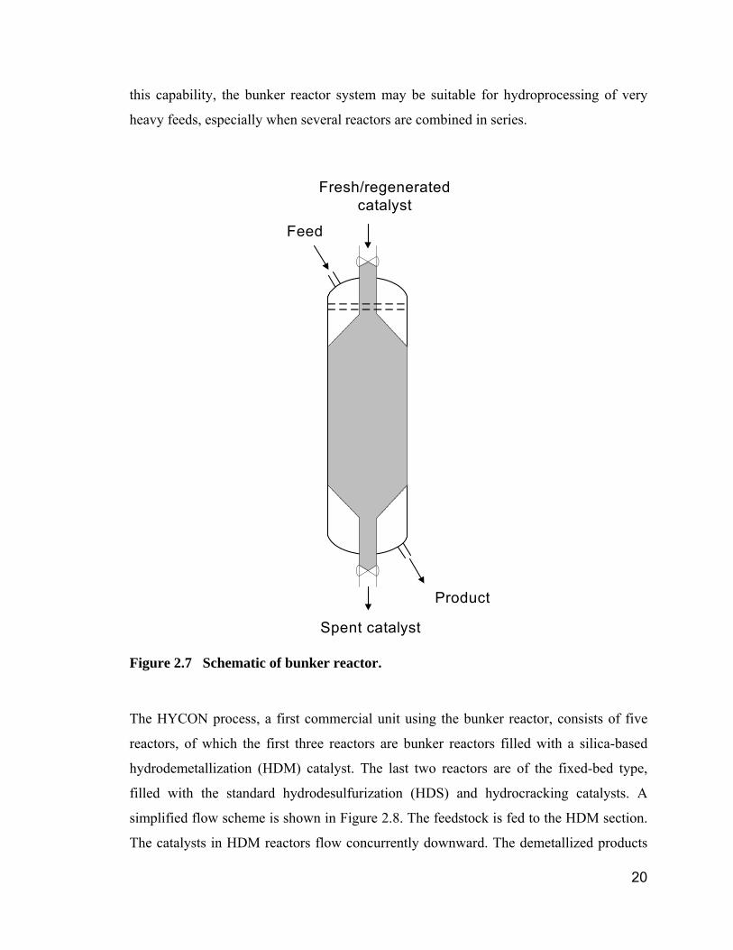
The HYCON process, a first commercial unit using the bunker reactor, consists of five
reactors, of which the first three reactors are bunker reactors filled with a silica-based
hydrodemetallization (HDM) catalyst. The last two reactors are of the fixed-bed type,
filled with the standard hydrodesulfurization (HDS) and hydrocracking catalysts. A
simplified flow scheme is shown in Figure 2.8. The feedstock is fed to the HDM section.
The catalysts in HDM reactors flow concurrently downward. The demetallized products
21
pass to the fixed bed HCON section where the product is further desulfurized and
converted.
catalyst catalyst
catalyst catalyst
Quench hydrogen
Effluent to fractionation
catalyst
catalyst
Feed
HDM section HCON section
Figure 2.8 Process flow scheme of the HYCON unit.
The other moving bed processes include OCR (On-stream Catalyst Replacement) process
licensed by Chevron and HYVAHL-M process licensed by IFP (Morel et al. 1997). Both
of these two processes adopt the counter-current moving bed reactor where the catalyst
circulates from top to bottom of the reactor while the reaction fluids circulate from
bottom to top in counter-current to the catalyst. The counter-current configuration is
better than the co-current configuration adopted in the bunker reactor since the spent
catalyst saturated by metals meet the fresh feed at the bottom of the reactor whereas the
fresh catalyst reacts with an already demetallized feed at the top of the reactor. This
configuration results in a lower catalyst consumption.
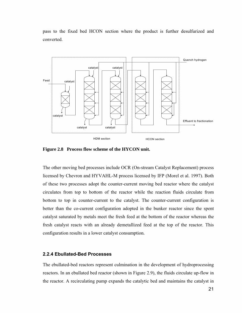
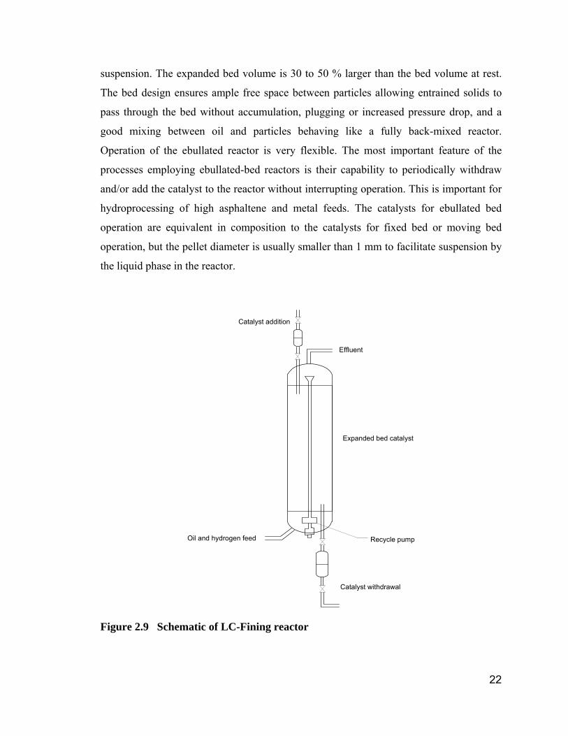
2.2.4 Ebullated-Bed Processes
The ebullated-bed reactors represent culmination in the development of hydroprocessing
reactors. In an ebullated bed reactor (shown in Figure 2.9), the fluids circulate up-flow in
the reactor. A recirculating pump expands the catalytic bed and maintains the catalyst in
22
suspension. The expanded bed volume is 30 to 50 % larger than the bed volume at rest.
The bed design ensures ample free space between particles allowing entrained solids to
pass through the bed without accumulation, plugging or increased pressure drop, and a
good mixing between oil and particles behaving like a fully back-mixed reactor.
Operation of the ebullated reactor is very flexible. The most important feature of the
processes employing ebullated-bed reactors is their capability to periodically withdraw
and/or add the catalyst to the reactor without interrupting operation. This is important for
hydroprocessing of high asphaltene and metal feeds. The catalysts for ebullated bed
operation are equivalent in composition to the catalysts for fixed bed or moving bed
operation, but the pellet diameter is usually smaller than 1 mm to facilitate suspension by
the liquid phase in the reactor.
Expanded bed catalyst
Effluent
Catalyst withdrawal
Oil and hydrogen feed
Catalyst addition
Recycle pump
Figure 2.9 Schematic of LC-Fining reactor
23
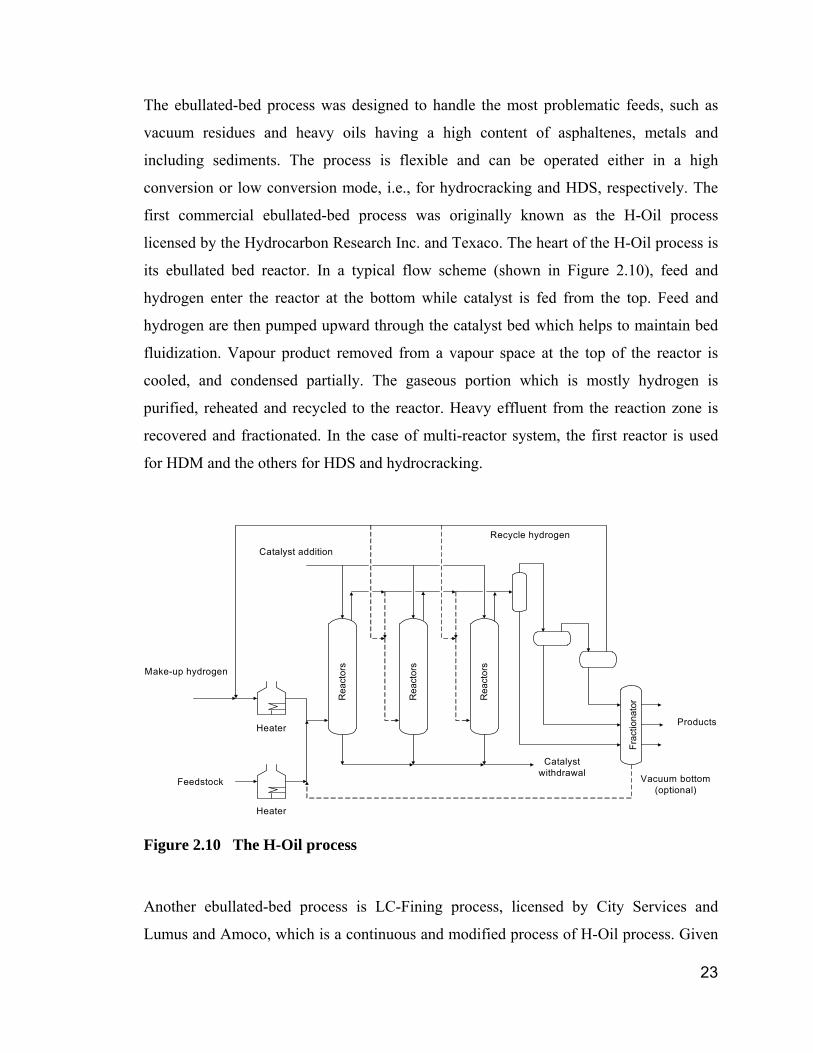
The ebullated-bed process was designed to handle the most problematic feeds, such as
vacuum residues and heavy oils having a high content of asphaltenes, metals and
including sediments. The process is flexible and can be operated either in a high
conversion or low conversion mode, i.e., for hydrocracking and HDS, respectively. The
first commercial ebullated-bed process was originally known as the H-Oil process
licensed by the Hydrocarbon Research Inc. and Texaco. The heart of the H-Oil process is
its ebullated bed reactor. In a typical flow scheme (shown in Figure 2.10), feed and
hydrogen enter the reactor at the bottom while catalyst is fed from the top. Feed and
hydrogen are then pumped upward through the catalyst bed which helps to maintain bed
fluidization. Vapour product removed from a vapour space at the top of the reactor is
cooled, and condensed partially. The gaseous portion which is mostly hydrogen is
purified, reheated and recycled to the reactor. Heavy effluent from the reaction zone is
recovered and fractionated. In the case of multi-reactor system, the first reactor is used
for HDM and the others for HDS and hydrocracking.
Make-up hydrogen
Feedstock
Heater
Rea
ctor
s
Heater
Frac
tiona
tor
Products
Rea
ctor
s
Rea
ctor
s
Catalyst addition
Catalyst withdrawal Vacuum bottom
(optional)
Recycle hydrogen
Figure 2.10 The H-Oil process
Another ebullated-bed process is LC-Fining process, licensed by City Services and
Lumus and Amoco, which is a continuous and modified process of H-Oil process. Given
24
the history of the development of the ebullated process, the features of both the LC-
Fining process and the H-Oil process are very similar. Nevertheless, the information
available in the literature is divided as to refer to these processes separately. Several
commercial H-Oil and LC-Fining units are in operation in different parts of the world.
2.2.5 Slurry Phase Process
The slurry phase processes, an alternative to fixed-, moving-, and ebullated-bed catalytic
processing, employs disposable catalysts such as finely divided solids. The once-through
catalyst is slurried with the feed prior to entering the reactor, a free-internal-equipment
tubular reactor, where the liquid or liquid suspension of additive flows upward with the
hydrogen gas. After reaction, the catalyst remains in the unconverted residue fraction.
The recovery of the highly dispersed catalyst is usually not practical and the catalyst is
inexpensive such that the catalyst is discarded. Among the most attractive features of
slurry-phase operation are the limited amount of catalyst required to achieve the desired
conversions, and the simplicity, high efficiency, and improved temperature control
possibilities of the reactor vessel. So this process is not attempting simultaneous
hydrodesulfurization (HDS), hydrodenitrogenation (HDN), hydrodemetallization (HDM),
and cracking conversion in a single reactor. The HDS, HDN is achieved in the
downstream reactors. This technology boasts being able to handle a wide feed stock
variability, and very high metals, high asphaltene and CCR content.
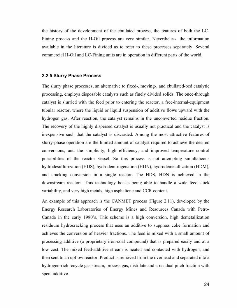
An example of this approach is the CANMET process (Figure 2.11), developed by the
Energy Research Laboratories of Energy Mines and Resources Canada with Petro-
Canada in the early 1980’s. This scheme is a high conversion, high demetallization
residuum hydrocracking process that uses an additive to suppress coke formation and
achieves the conversion of heavier fractions. The feed is mixed with a small amount of
processing additive (a proprietary iron-coal compound) that is prepared easily and at a
low cost. The mixed feed-additive stream is heated and contacted with hydrogen, and
then sent to an upflow reactor. Product is removed from the overhead and separated into a
hydrogen-rich recycle gas stream, process gas, distillate and a residual pitch fraction with
spent additive.
25
Hydrogen
Feedstock
Heater
Rea
ctor
s
HeaterAdditive
Frac
tiona
tor
Products
Figure 2.11 The CANMET process
2.2.6 Catalyst Characteristics
Regarding the granular catalysts, a wide range of hydroprocessing catalysts have been
developed for commercial applications. The major group includes supported molybdate
and tungstate catalysts promoted by either Ni or Co. γ-Alumina is the common support.
Since the presence of large quantities of asphaltenes, S, N, and O as well as metals such
as Ni, V, Ti, Fe and others in the heavy oils, the catalysts must possess a high activity and
at the same time be tolerant to metals. The physical properties of catalysts must be
thoroughly considered. Special attention has to be paid to the size of the particles, pore
volume and size distribution, pore diameter and the shape of the particles to maximize the
utilization of the catalyst. For a heavy oil feed, if the catalyst mean pore diameter is in the
neighbourhood of the size of resins and asphaltenes of the feed, the diffusion rate is much
slower than the reaction rate, and only part of the catalyst particles is used and metals are
deposited on the outside of the catalyst particles. Catalysts with larger pores are required
for hydroprocessing of such a feed, but at the expense of the catalyst activity due to the
loss of surface area. The influence of pore sizes on radial distribution of metal deposition
is illustrated in Figure 2.12. Usually there is an optimum pore size distribution for a given
feed to a given process. A proper combination of porosity, surface area and activity
becomes an important task in the development of hydroprocessing catalysts for heavy
oils.
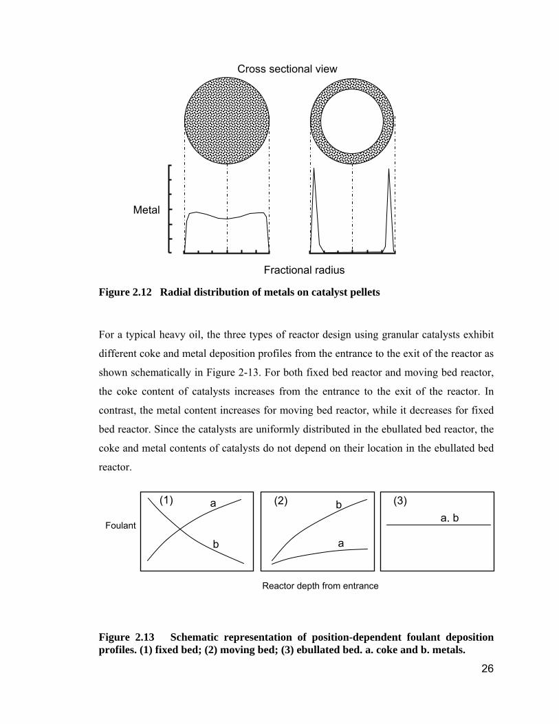
26
Figure 2.12 Radial distribution of metals on catalyst pellets
For a typical heavy oil, the three types of reactor design using granular catalysts exhibit
different coke and metal deposition profiles from the entrance to the exit of the reactor as
shown schematically in Figure 2-13. For both fixed bed reactor and moving bed reactor,
the coke content of catalysts increases from the entrance to the exit of the reactor. In
contrast, the metal content increases for moving bed reactor, while it decreases for fixed
bed reactor. Since the catalysts are uniformly distributed in the ebullated bed reactor, the
coke and metal contents of catalysts do not depend on their location in the ebullated bed
reactor.
Figure 2.13 Schematic representation of position-dependent foulant deposition profiles. (1) fixed bed; (2) moving bed; (3) ebullated bed. a. coke and b. metals.
Foulant
Reactor depth from entrance
a
b a
a, bb(2) (3) (1)
Metal
Fractional radius
Cross sectional view
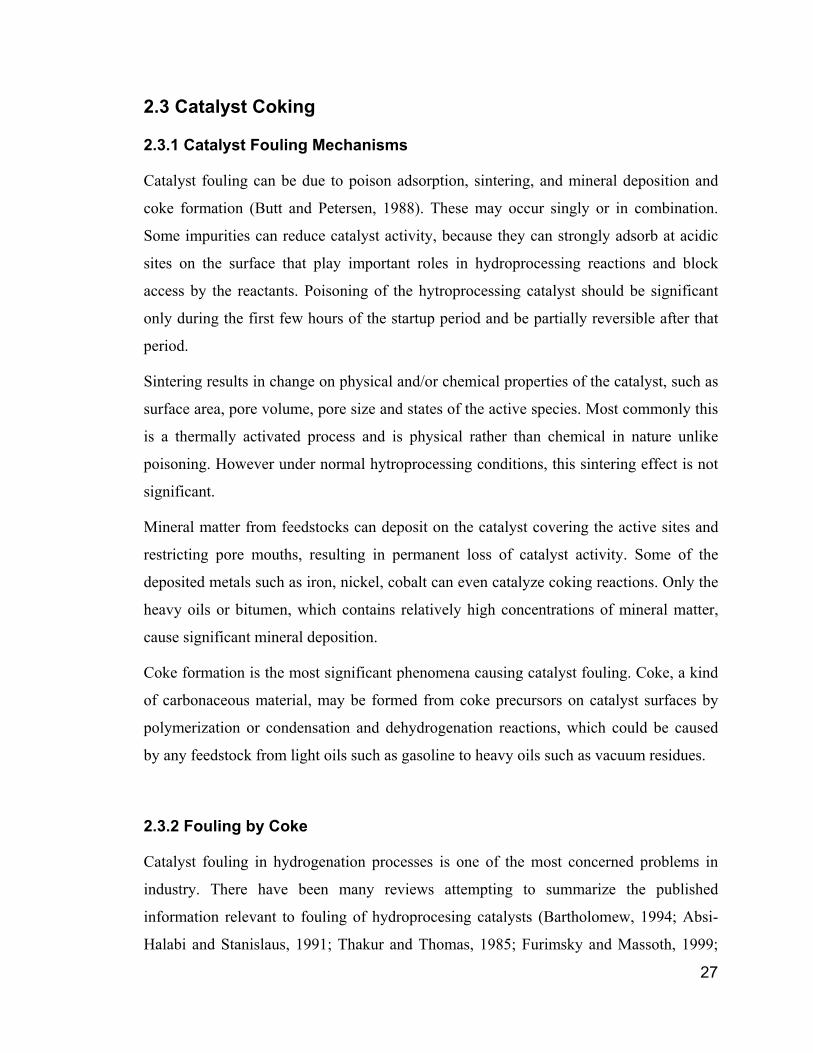
27
2.3 Catalyst Coking
2.3.1 Catalyst Fouling Mechanisms
Catalyst fouling can be due to poison adsorption, sintering, and mineral deposition and
coke formation (Butt and Petersen, 1988). These may occur singly or in combination.
Some impurities can reduce catalyst activity, because they can strongly adsorb at acidic
sites on the surface that play important roles in hydroprocessing reactions and block
access by the reactants. Poisoning of the hytroprocessing catalyst should be significant
only during the first few hours of the startup period and be partially reversible after that
period.
Sintering results in change on physical and/or chemical properties of the catalyst, such as
surface area, pore volume, pore size and states of the active species. Most commonly this
is a thermally activated process and is physical rather than chemical in nature unlike
poisoning. However under normal hytroprocessing conditions, this sintering effect is not
significant.
Mineral matter from feedstocks can deposit on the catalyst covering the active sites and
restricting pore mouths, resulting in permanent loss of catalyst activity. Some of the
deposited metals such as iron, nickel, cobalt can even catalyze coking reactions. Only the
heavy oils or bitumen, which contains relatively high concentrations of mineral matter,
cause significant mineral deposition.
Coke formation is the most significant phenomena causing catalyst fouling. Coke, a kind
of carbonaceous material, may be formed from coke precursors on catalyst surfaces by
polymerization or condensation and dehydrogenation reactions, which could be caused
by any feedstock from light oils such as gasoline to heavy oils such as vacuum residues.
2.3.2 Fouling by Coke
Catalyst fouling in hydrogenation processes is one of the most concerned problems in
industry. There have been many reviews attempting to summarize the published
information relevant to fouling of hydroprocesing catalysts (Bartholomew, 1994; Absi-
Halabi and Stanislaus, 1991; Thakur and Thomas, 1985; Furimsky and Massoth, 1999;
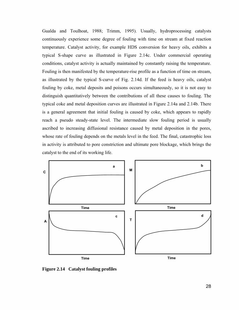
28
Gualda and Toulhoat, 1988; Trimm, 1995). Usually, hydroprocessing catalysts
continuously experience some degree of fouling with time on stream at fixed reaction
temperature. Catalyst activity, for example HDS conversion for heavy oils, exhibits a
typical S-shape curve as illustrated in Figure 2.14c. Under commercial operating
conditions, catalyst activity is actually maintained by constantly raising the temperature.
Fouling is then manifested by the temperature-rise profile as a function of time on stream,
as illustrated by the typical S-curve of Fig. 2.14d. If the feed is heavy oils, catalyst
fouling by coke, metal deposits and poisons occurs simultaneously, so it is not easy to
distinguish quantitatively between the contributions of all these causes to fouling. The
typical coke and metal deposition curves are illustrated in Figure 2.14a and 2.14b. There
is a general agreement that initial fouling is caused by coke, which appears to rapidly
reach a pseudo steady-state level. The intermediate slow fouling period is usually
ascribed to increasing diffusional resistance caused by metal deposition in the pores,
whose rate of fouling depends on the metals level in the feed. The final, catastrophic loss
in activity is attributed to pore constriction and ultimate pore blockage, which brings the
catalyst to the end of its working life.
Figure 2.14 Catalyst fouling profiles
Time
Ca
Time
Mb
Time
Td
Time
Ac
29
During the start-up phase in hydroprocessing, initial coke deposition is one of the most
significant factors influencing catalyst fouling. Several studies, focusing on the initial
catalyst coking, indicate that coke deposition is believed to be very fast in the initial
period of operation, particularly, in residual oil hydroprocessing (Marafi and Stanislaus,
2001; Matsushita et al. 2004; Hauser et al. 2005; Richardson et al. 1996; Idei et al. 2002;
Gualda and Kasztelan, 1996). Approximately 50 wt% of the total deposited carbon is laid
down on the catalyst within the first few days of operation (Hauser et al. 2005). Much of
coke formed during the early hours of the run is deposited in micropores of the catalyst
leading to a substantial loss in surface area and pore volume (Absi-Halabi et al., 1991;
Callejas et al. 2001; Marafi and Stanislaus, 2001). And at the early stage of operation,
much of coke on catalyst is reversible species not only in terms of composition but also in
terms of quantity (Callejas et al. 2001; Gualda and Kasztelan, 1996). The reversible coke
can be easily removed or reversed if a proper operation is applied. The irreversible coke,
strongly adsorbed at the support surface, is deposited on catalyst even at the very early
state, and the ratio of irreversible coke to reversible coke increases with time on stream.
As the time on stream increases, the coke becomes more aromatic, exhibiting in a
decrease of H/C ratio.(Matsushita et al. 2004; Hauser et al. 2005; Gualda and Kasztelan,
1996).
2.3.3 Coke Formation Chemistry
The structure of coke and the mechanisms of coke formation are complex and not fully
understood. Coke is not a well-defined substance; normally it has an empirical formula
approximating CH, but the chemical nature depends very much on how it is formed.
Coke is formed via two parallel routes, viz. (i) thermal polymerization or condensation
reactions and (ii) catalytic dehydrogenation reactions (de Jong, et al., 1994b). The
catalyst composition has a large impact on the amount of catalytic coke whilst physical
effects (phase equilibrium) predominate in determining the extent of thermal coke
formation. Coke formation on catalysts may take several forms and be caused by
different mechanisms. From the nature and shape, coke is normally classified into three
main types: amorphous, filamentous and graphite platelets (Hughes, 1984; Butt and
30
Petersen, 1988; Absi-Halabi et al., 1991). These types would not be distinguished during
a routine analysis of the spent catalysts, but merely referred to collectively as “coke”.
Condensation and polymerization reactions play a major role in amorphous coke
formation. Although some hydrogen is removed during condensation, a significant
amount still remains in the deposit. As the temperature is raised, dehydrogenation
reactions reduce the hydrogen content. Filamentous coke is produced by the catalytic
decomposition of carbon containing gases on small metal particles such as iron, cobalt
and nickel and their oxides. The graphitic deposit is formed indirectly, at the expense of
the other two deposit forms and also requires the participation of a catalyst. The graphite
carbon can form only at elevated temperature higher than 1000°C. Therefore, only
amorphous and filamentous types of coke deposits are significant in hydroprocessing
catalysts.
The species acting as precursors for coke have been the subject of much investigation and
speculation. Among hydrocarbons, the alkenes and aromatics (associated with or without
heteroatoms) are the generally agreed upon coke precursors. The interaction of aromatics
or alkene with the catalyst surface is much stronger than that of saturated hydrocarbons.
Therefore they are more likely to convert to higher molecular weight species by
polymerization or condensation if sufficient active hydrogen is not available to prevent it.
The majority of opinion is in favor of aromatic species as the major coke precursor for
heavy oils hydroprocessing (Hughes, 1984). Especially, polar heteroaromatic compounds
having strong adsorption tendency and having high cracking and condensation reactivity
tend to form more coke, which is evident that the heteroatoms content in coke is higher
than in the feed. The aromatics could be present in the feedstock or may form as
intermediates in the hydrogenation process.
In the case of heavy feeds where asphaltenes are present, significant coke deposition can
be formed on the catalyst and the deposited carbon on spent catalyst is proportional to the
concentration of asphaltenes in feed (Gray et al. 1999). Studies have shown that
asphaltenes are a major contributor to coke formation in the hydroprocessing of heavy
oils (Absi-Halabi et al., 1991; Marafi and Stanislaus, 2001; Gray et al. 1999). They have
a higher propensity to form coke by directly depositing on catalyst as coke precursor
themselves, or by generating condensed aromatics via cracking off side chains.
31
2.3.4 Coke Deposition Modes
In regard to catalyst fouling mechanisms and catalyst bed fouling, one could apply
another classification to interpret coke deposition in hydroprocessing. Uniform surface
deposition (Richardson et al. 1996), pore-mouth plugging (Muegge and Massoth, 1991),
and bulk phase coke deposition (Richardson et al. 1996) are three observed modes for
coke deposition (Figure 1.1). Uniform surface deposition and pore mouth plugging
models are two hotly-debated models because conflicting results were reported on the
probable location of coke deposits in hydroprocessing catalysts. Richardson et al. (1996)
suggest that coke deposits uniformly on catalyst surfaces with monolayer coverage.
Deposition beyond a molecular monolayer is not accounted for in this modelling
approach. Typical experimental findings that suggest uniform surface deposition show a
loss of pore volume for only the smallest pores, a gradual decrease in catalyst surface
area, and a gradual decrease in pore volume as overall coke content increases, thus
affecting the smallest pores (with highest surface area to volume ratios) before affecting
larger pores. The other experimental findings by Ternan et al. (1979), Diez et al. (1990)
also support this model.
Muegge and Massoth (1991) studied the effect of coke produced from a model-coke
precursor, anthracene, on the physical properties of a catalyst. Examination of pore
structures indicated that the loss of pore volume and surface area was due to pore
blockage, but the small pores, expected to be blocked, were not preferentially blocked.
And the inconsistency between the significant lowering in diffusivity and the small
change in average pore radius at higher coke deposition revealed that a wedge-like
growth of coke deposit at pore mouth must occur before the pore-mouth plugging. The
pore mouth plugging is also experimentally observed at initial rapid coke deposition stage
(Absi-Halabi et al. 1991). Lee et al. (1991a) also observed a drastic reduction in
diffusivity due to a small amount of coke deposition, indicating that in some cases, the
pore network in the catalyst can be blocked at the pore mouth. This model, based on
experiments, is consistent with localized multilayer deposition and is inconsistent with
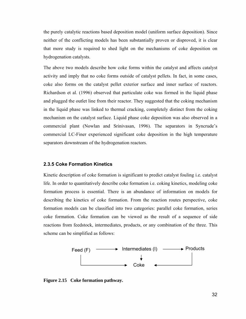
32
the purely catalytic reactions based deposition model (uniform surface deposition). Since
neither of the conflicting models has been substantially proven or disproved, it is clear
that more study is required to shed light on the mechanisms of coke deposition on
hydrogenation catalysts.
The above two models describe how coke forms within the catalyst and affects catalyst
activity and imply that no coke forms outside of catalyst pellets. In fact, in some cases,
coke also forms on the catalyst pellet exterior surface and inner surface of reactors.
Richardson et al. (1996) observed that particulate coke was formed in the liquid phase
and plugged the outlet line from their reactor. They suggested that the coking mechanism
in the liquid phase was linked to thermal cracking, completely distinct from the coking
mechanism on the catalyst surface. Liquid phase coke deposition was also observed in a
commercial plant (Nowlan and Srinivasan, 1996). The separators in Syncrude’s
commercial LC-Finer experienced significant coke deposition in the high temperature
separators downstream of the hydrogenation reactors.
2.3.5 Coke Formation Kinetics
Kinetic description of coke formation is significant to predict catalyst fouling i.e. catalyst
life. In order to quantitatively describe coke formation i.e. coking kinetics, modeling coke
formation process is essential. There is an abundance of information on models for
describing the kinetics of coke formation. From the reaction routes perspective, coke
formation models can be classified into two categories: parallel coke formation, series
coke formation. Coke formation can be viewed as the result of a sequence of side
reactions from feedstock, intermediates, products, or any combination of the three. This
scheme can be simplified as follows:
Figure 2.15 Coke formation pathway.
Feed (F) Intermediates (I) Products
Coke
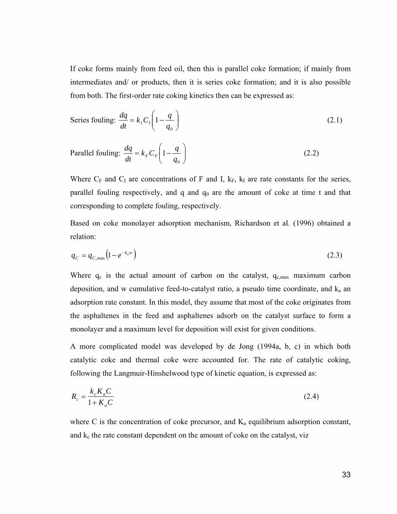
33
If coke forms mainly from feed oil, then this is parallel coke formation; if mainly from
intermediates and/ or products, then it is series coke formation; and it is also possible
from both. The first-order rate coking kinetics then can be expressed as:
Series fouling: ⎟⎟⎠
⎞⎜⎜⎝
⎛−=
0
1qqCk
dtdq
II (2.1)
Parallel fouling: ⎟⎟⎠
⎞⎜⎜⎝
⎛−=
0
1qqCk
dtdq
FF (2.2)
Where CF and CI are concentrations of F and I, kF, kI are rate constants for the series,
parallel fouling respectively, and q and q0 are the amount of coke at time t and that
corresponding to complete fouling, respectively.
Based on coke monolayer adsorption mechanism, Richardson et al. (1996) obtained a
relation:
( )wkCC
aeqq −−= 1max, (2.3)
Where qc is the actual amount of carbon on the catalyst, qc,max maximum carbon
deposition, and w cumulative feed-to-catalyst ratio, a pseudo time coordinate, and ka an
adsorption rate constant. In this model, they assume that most of the coke originates from
the asphaltenes in the feed and asphaltenes adsorb on the catalyst surface to form a
monolayer and a maximum level for deposition will exist for given conditions.
A more complicated model was developed by de Jong (1994a, b, c) in which both
catalytic coke and thermal coke were accounted for. The rate of catalytic coking,
following the Langmuir-Hinshelwood type of kinetic equation, is expressed as:
CKCKk
Ra
acc +=
1 (2.4)
where C is the concentration of coke precursor, and Ka equilibrium adsorption constant,
and kc the rate constant dependent on the amount of coke on the catalyst, viz
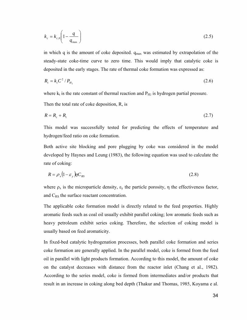
34
⎟⎟⎠
⎞⎜⎜⎝
⎛−=
max0, 1
qqkk cc (2.5)
in which q is the amount of coke deposited. qmax was estimated by extrapolation of the
steady-state coke-time curve to zero time. This would imply that catalytic coke is
deposited in the early stages. The rate of thermal coke formation was expressed as:
2/2
Htt PCkR = (2.6)
where kt is the rate constant of thermal reaction and PH2 is hydrogen partial pressure.
Then the total rate of coke deposition, R, is
tc RRR += (2.7)
This model was successfully tested for predicting the effects of temperature and
hydrogen/feed ratio on coke formation.
Both active site blocking and pore plugging by coke was considered in the model
developed by Haynes and Leung (1983), the following equation was used to calculate the
rate of coking:
( ) RSyx CR ηερ −= 1 (2.8)
where ρx is the microparticle density, εy the particle porosity, η the effectiveness factor,
and CRS the surface reactant concentration.
The applicable coke formation model is directly related to the feed properties. Highly
aromatic feeds such as coal oil usually exhibit parallel coking; low aromatic feeds such as
heavy petroleum exhibit series coking. Therefore, the selection of coking model is
usually based on feed aromaticity.
In fixed-bed catalytic hydrogenation processes, both parallel coke formation and series
coke formation are generally applied. In the parallel model, coke is formed from the feed
oil in parallel with light products formation. According to this model, the amount of coke
on the catalyst decreases with distance from the reactor inlet (Chang et al., 1982).
According to the series model, coke is formed from intermediates and/or products that
result in an increase in coking along bed depth (Thakur and Thomas, 1985, Koyama e al.
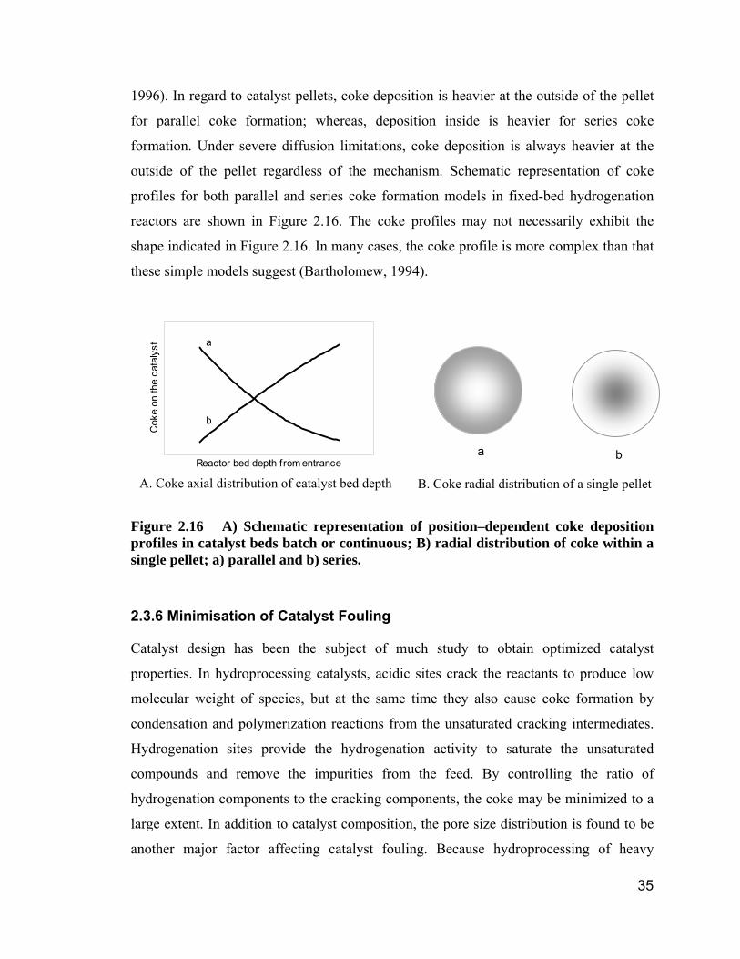
35
1996). In regard to catalyst pellets, coke deposition is heavier at the outside of the pellet
for parallel coke formation; whereas, deposition inside is heavier for series coke
formation. Under severe diffusion limitations, coke deposition is always heavier at the
outside of the pellet regardless of the mechanism. Schematic representation of coke
profiles for both parallel and series coke formation models in fixed-bed hydrogenation
reactors are shown in Figure 2.16. The coke profiles may not necessarily exhibit the
shape indicated in Figure 2.16. In many cases, the coke profile is more complex than that
these simple models suggest (Bartholomew, 1994).
Figure 2.16 A) Schematic representation of position–dependent coke deposition profiles in catalyst beds batch or continuous; B) radial distribution of coke within a single pellet; a) parallel and b) series.
2.3.6 Minimisation of Catalyst Fouling
Catalyst design has been the subject of much study to obtain optimized catalyst
properties. In hydroprocessing catalysts, acidic sites crack the reactants to produce low
molecular weight of species, but at the same time they also cause coke formation by
condensation and polymerization reactions from the unsaturated cracking intermediates.
Hydrogenation sites provide the hydrogenation activity to saturate the unsaturated
compounds and remove the impurities from the feed. By controlling the ratio of
hydrogenation components to the cracking components, the coke may be minimized to a
large extent. In addition to catalyst composition, the pore size distribution is found to be
another major factor affecting catalyst fouling. Because hydroprocessing of heavy
Reactor bed depth from entrance
Cok
e on
the
cata
lyst
b
a
a b
A. Coke axial distribution of catalyst bed depth B. Coke radial distribution of a single pellet
36
feedstocks is a diffusion-controlled process, micropores are not accessible to large
molecules like asphaletenes and are easily blocked by the coke formed at a pore mouth
(pore mouth plugging). An optimum catalyst pore structure facilitates access of reactants
to the interior of the catalyst and reduces catalyst fouling due to pore mouth plugging and
at the same time provides enough catalyst surfaces for reaction. The size of catalyst
pellets may also affect the effectiveness of a catalyst. By decreasing particle size, catalyst
may be utilized more effectively by avoiding the egg-white coke deposition. However,
small particle sizes lead to increased pressure drop and serious bed plugging in a fixed
bed reactor. An optimum particle size is a 0.8 to 1.6mm diameter extruded cylindrical
pellet (Thakur and Thomas, 1985).
Operating conditions can also be adjusted to minimize coking. Under severe operating
conditions such as high space velocities, high temperature and low hydrogen pressure,
coke forms much faster thereby resulting in rapid catalyst fouling. It is very easy to
understand why high space velocities cause high coking rates in that the coke precursor
amount passing through the catalyst is higher for high space velocities than at low space
velocities. High reaction temperatures yield higher free radical concentrations which may
cause high coking rates if they are not saturated. An increase in hydrogen pressure has a
favourable effect if catalyst fouling is caused by coke formation, because the free radical
intermediates which form coke can be saturated by hydrogen before coke can form. The
hydrogen to oil ratio is another important parameter in hydroprocessing. Coke extents
pass through a maximum going from low to high ratios. This is due to the existence of a
critical condition, that is, a dew point for the fluid inside the reactor (de Jong et al., 1994).
Catalyst fouling increases with the molecular weight/boiling point of the feedstock. By
controlling the feed into a reactor, coke formation may be reduced. For example, high
molecular weight of asphaltene is the major source of coke, and pre-treatment of the feed
by solvent deasphalting leads to a major reduction in coke formation.
Another approach to reduce coke formation is by modifying the composition of the feed
mixture or the recycle (Gray, 1994). The addition of hydrogenated heavy aromatic
petroleum fractions or heavy aromatic petroleum fractions suppresses coke formation by
providing a medium with high hydrogen solubility and which reduces hydrogen
consumption (Kubo et al., 1994 and 1996). The success of this approach is normally
37
attributed to enhanced hydrogen transfer from the vapour phase to the oil phase and the
high radical scavenging ability of additives (Kubo et al., 1994). Another explanation for
coke reduction by adding solvent to a feed is the solubility increase due to the solvent
addition makes the more solid soluble in the fluid and therefore suppresses the coke
formation (Gray, 1994). Supercritical conditions caused by adding a solvent to the feed
also reduce coke formation in upgrading of heavy oil (Scotta et al., 2001). Diffusion rates
of supercritical fluids into catalyst pores are much higher than those for subcritical
systems (Lee, et al. 1991a, 1991b), and an optimum fluid density which minimizes coke
deposition and mass transfer limitations can be expected to exist at supercritical or near-
supercritical conditions (Baptist-Nguyen, and Subramanjam, 1992).
2.4 The Role of Phase Behaviour in Coke Formation
2.4.1 Introduction
Phase diagram and phase behaviour are often the starting point and base for designing or
developing many industrial processes. One of the most typical examples is the heavy oil
solvent deasphalting process (McHugh and Krukonis, 1994), which operates in the LLV
or LL multiphase phase region and produces purified light oil by getting rid of L2 - the
asphaltene rich phase. Liquid-liquid phase separation created by mixing light solvent and
heavy oil is a key to achieve upgrading of heavy oils. Some industrial processes such as
coking processes and solvent deasphalting processes try to take advantage of this kind of
phase separation, while some other processes such as visbreaking process have to avoid
the occurrence of phase separation. In heavy oil hydroprocessing, phase separation may
occur and cause serious coke formation. Phase diagrams and the evolution of phase
diagrams as reactions progress in heavy oil hydroprocessing may provide key insights
into the coke formation mechanism. Therefore, understanding phase behaviour is crucial
to the design and development of industrial processes.
2.4.2 Some Basic Theories of Phase Behaviour
2.4.2.1 Fluid Phase Behaviours
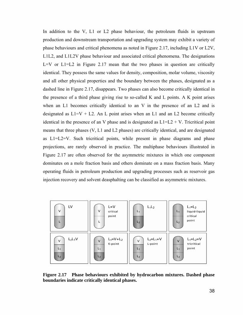
38
In addition to the V, L1 or L2 phase behaviour, the petroleum fluids in upstream
production and downstream transportation and upgrading system may exhibit a variety of
phase behaviours and critical phenomena as noted in Figure 2.17, including L1V or L2V,
L1L2, and L1L2V phase behaviour and associated critical phenomena. The designations
L=V or L1=L2 in Figure 2.17 mean that the two phases in question are critically
identical. They possess the same values for density, composition, molar volume, viscosity
and all other physical properties and the boundary between the phases, designated as a
dashed line in Figure 2.17, disappears. Two phases can also become critically identical in
the presence of a third phase giving rise to so-called K and L points. A K point arises
when an L1 becomes critically identical to an V in the presence of an L2 and is
designated as L1=V + L2. An L point arises when an L1 and an L2 become critically
identical in the presence of an V phase and is designated as L1=L2 + V. Tricritical point
means that three phases (V, L1 and L2 phases) are critically identical, and are designated
as L1=L2=V. Such tricritical points, while present in phase diagrams and phase
projections, are rarely observed in practice. The multiphase behaviours illustrated in
Figure 2.17 are often observed for the asymmetric mixtures in which one component
dominates on a mole fraction basis and others dominate on a mass fraction basis. Many
operating fluids in petroleum production and upgrading processes such as reservoir gas
injection recovery and solvent deasphalting can be classified as asymmetric mixtures.
Figure 2.17 Phase behaviours exhibited by hydrocarbon mixtures. Dashed phase boundaries indicate critically identical phases.
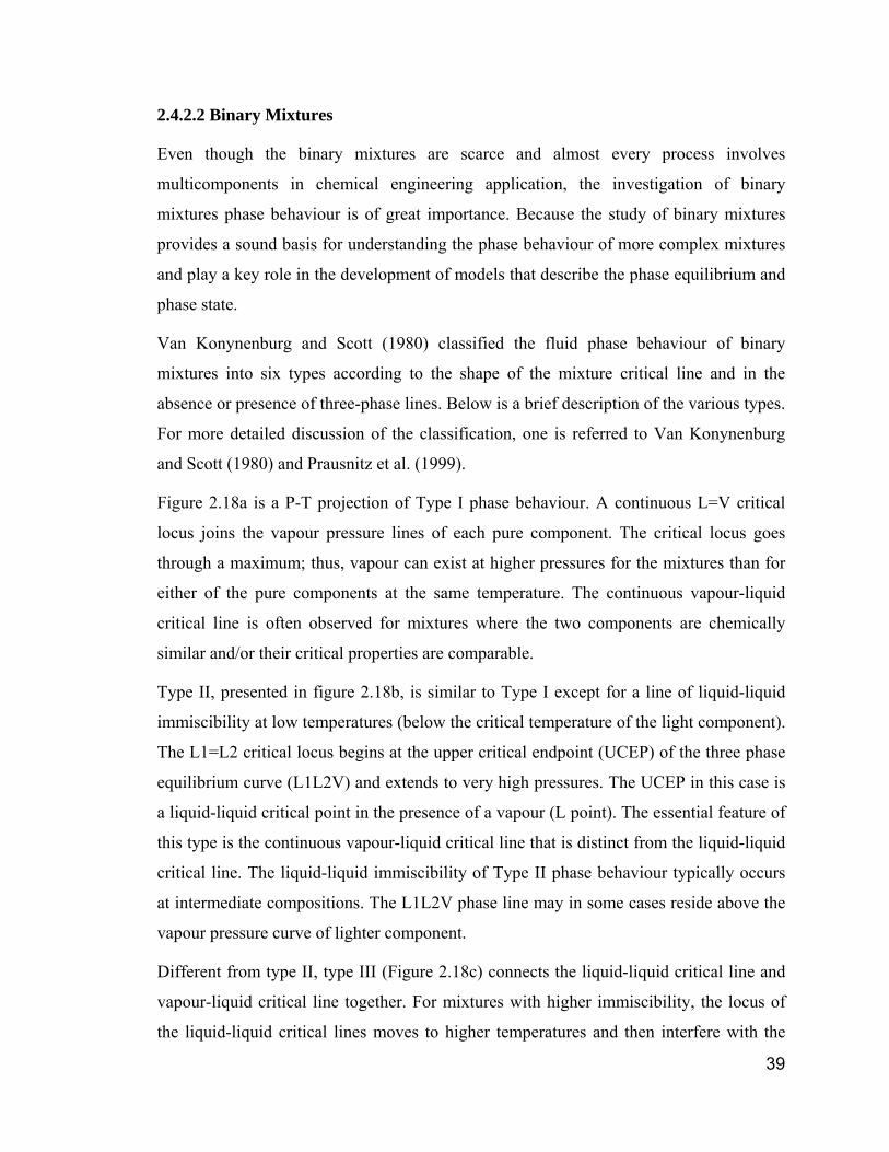
39
2.4.2.2 Binary Mixtures
Even though the binary mixtures are scarce and almost every process involves
multicomponents in chemical engineering application, the investigation of binary
mixtures phase behaviour is of great importance. Because the study of binary mixtures
provides a sound basis for understanding the phase behaviour of more complex mixtures
and play a key role in the development of models that describe the phase equilibrium and
phase state.
Van Konynenburg and Scott (1980) classified the fluid phase behaviour of binary
mixtures into six types according to the shape of the mixture critical line and in the
absence or presence of three-phase lines. Below is a brief description of the various types.
For more detailed discussion of the classification, one is referred to Van Konynenburg
and Scott (1980) and Prausnitz et al. (1999).
Figure 2.18a is a P-T projection of Type I phase behaviour. A continuous L=V critical
locus joins the vapour pressure lines of each pure component. The critical locus goes
through a maximum; thus, vapour can exist at higher pressures for the mixtures than for
either of the pure components at the same temperature. The continuous vapour-liquid
critical line is often observed for mixtures where the two components are chemically
similar and/or their critical properties are comparable.
Type II, presented in figure 2.18b, is similar to Type I except for a line of liquid-liquid
immiscibility at low temperatures (below the critical temperature of the light component).
The L1=L2 critical locus begins at the upper critical endpoint (UCEP) of the three phase
equilibrium curve (L1L2V) and extends to very high pressures. The UCEP in this case is
a liquid-liquid critical point in the presence of a vapour (L point). The essential feature of
this type is the continuous vapour-liquid critical line that is distinct from the liquid-liquid
critical line. The liquid-liquid immiscibility of Type II phase behaviour typically occurs
at intermediate compositions. The L1L2V phase line may in some cases reside above the
vapour pressure curve of lighter component.
Different from type II, type III (Figure 2.18c) connects the liquid-liquid critical line and
vapour-liquid critical line together. For mixtures with higher immiscibility, the locus of
the liquid-liquid critical lines moves to higher temperatures and then interfere with the
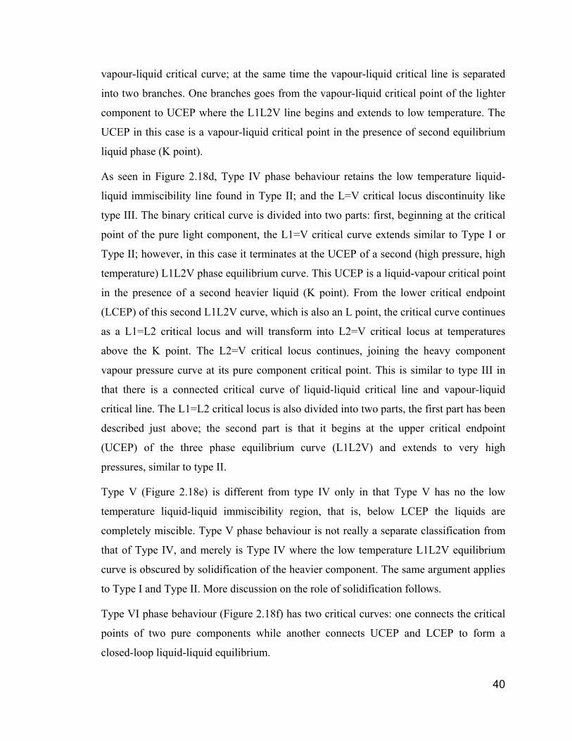
40
vapour-liquid critical curve; at the same time the vapour-liquid critical line is separated
into two branches. One branches goes from the vapour-liquid critical point of the lighter
component to UCEP where the L1L2V line begins and extends to low temperature. The
UCEP in this case is a vapour-liquid critical point in the presence of second equilibrium
liquid phase (K point).
As seen in Figure 2.18d, Type IV phase behaviour retains the low temperature liquid-
liquid immiscibility line found in Type II; and the L=V critical locus discontinuity like
type III. The binary critical curve is divided into two parts: first, beginning at the critical
point of the pure light component, the L1=V critical curve extends similar to Type I or
Type II; however, in this case it terminates at the UCEP of a second (high pressure, high
temperature) L1L2V phase equilibrium curve. This UCEP is a liquid-vapour critical point
in the presence of a second heavier liquid (K point). From the lower critical endpoint
(LCEP) of this second L1L2V curve, which is also an L point, the critical curve continues
as a L1=L2 critical locus and will transform into L2=V critical locus at temperatures
above the K point. The L2=V critical locus continues, joining the heavy component
vapour pressure curve at its pure component critical point. This is similar to type III in
that there is a connected critical curve of liquid-liquid critical line and vapour-liquid
critical line. The L1=L2 critical locus is also divided into two parts, the first part has been
described just above; the second part is that it begins at the upper critical endpoint
(UCEP) of the three phase equilibrium curve (L1L2V) and extends to very high
pressures, similar to type II.
Type V (Figure 2.18e) is different from type IV only in that Type V has no the low
temperature liquid-liquid immiscibility region, that is, below LCEP the liquids are
completely miscible. Type V phase behaviour is not really a separate classification from
that of Type IV, and merely is Type IV where the low temperature L1L2V equilibrium
curve is obscured by solidification of the heavier component. The same argument applies
to Type I and Type II. More discussion on the role of solidification follows.
Type VI phase behaviour (Figure 2.18f) has two critical curves: one connects the critical
points of two pure components while another connects UCEP and LCEP to form a
closed-loop liquid-liquid equilibrium.
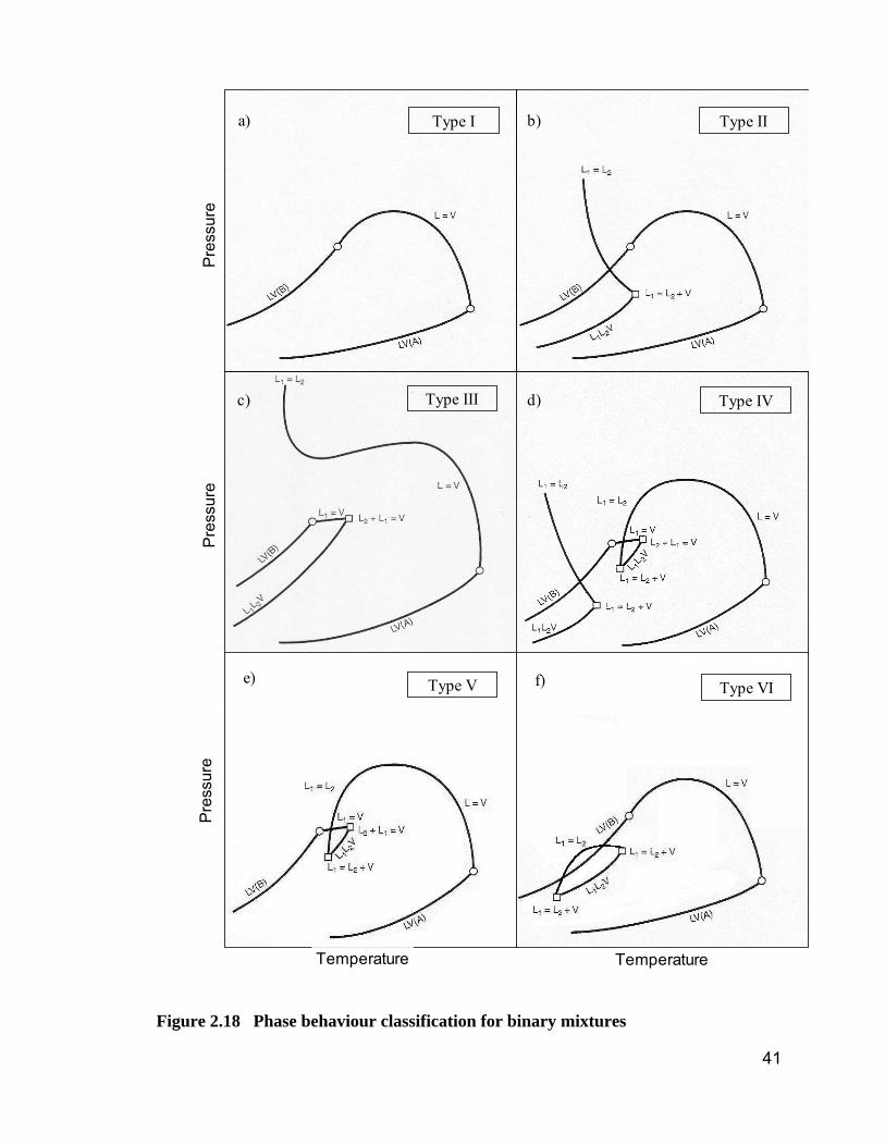
41
Figure 2.18 Phase behaviour classification for binary mixtures
Temperature
Pre
ssur
eP
ress
ure
Type I Type II
Type IV
Type V
a) b)
c) d)
Pre
ssur
e
Type VI
Type III
Temperature
e) f)
42
2.4.2.3 Ternary Mixtures
As the number of components is increased from two to three, LLV phase behaviour
extends over a region in pressure temperature space for any given ternary. Phase
diagrams for ternary systems are at least 4-dimensions. In practice, construction and
interpretation of phase diagrams of ternary systems are similar to and based on those of
binary systems.
Gregorowicz et al. (1993) reported detailed discussions on how to expand phase diagrams
of binary mixtures to phase diagrams of ternary mixtures. As an example, Type V phase
diagrams of a binary mixture shown in Figure 2.19 are expanded to ternary mixture phase
diagrams shown in Figure 2.20 when a miscible component for both components is
added.
Figure 2.19 Schematic Type V phase behaviour for a binary system. a: PTx three-dimensions; b: PT and Tx projections of the PTx three-dimensions
Figure 2.20a, b, c show the phase behaviour at mole fraction x1, x2, x3 as indicated in
Figure 2.19b, where x is the mole fraction of heavy component (A) and x1>x2>x3. For
P
x
T
a b
T
P
LV (A)
LV (B)
x1
L
K
LV(B)
LV(A)
L
K
K
L
B
A
x2
x3
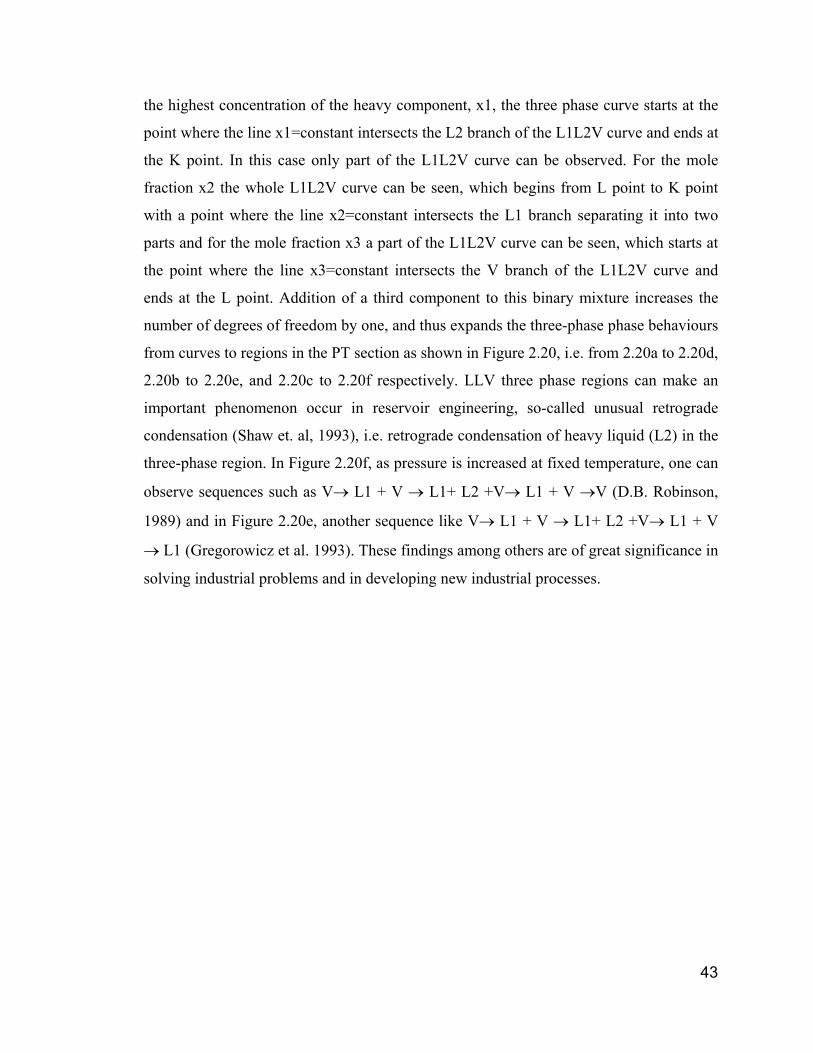
43
the highest concentration of the heavy component, x1, the three phase curve starts at the
point where the line x1=constant intersects the L2 branch of the L1L2V curve and ends at
the K point. In this case only part of the L1L2V curve can be observed. For the mole
fraction x2 the whole L1L2V curve can be seen, which begins from L point to K point
with a point where the line x2=constant intersects the L1 branch separating it into two
parts and for the mole fraction x3 a part of the L1L2V curve can be seen, which starts at
the point where the line x3=constant intersects the V branch of the L1L2V curve and
ends at the L point. Addition of a third component to this binary mixture increases the
number of degrees of freedom by one, and thus expands the three-phase phase behaviours
from curves to regions in the PT section as shown in Figure 2.20, i.e. from 2.20a to 2.20d,
2.20b to 2.20e, and 2.20c to 2.20f respectively. LLV three phase regions can make an
important phenomenon occur in reservoir engineering, so-called unusual retrograde
condensation (Shaw et. al, 1993), i.e. retrograde condensation of heavy liquid (L2) in the
three-phase region. In Figure 2.20f, as pressure is increased at fixed temperature, one can
observe sequences such as V→ L1 + V → L1+ L2 +V→ L1 + V →V (D.B. Robinson,
1989) and in Figure 2.20e, another sequence like V→ L1 + V → L1+ L2 +V→ L1 + V
→ L1 (Gregorowicz et al. 1993). These findings among others are of great significance in
solving industrial problems and in developing new industrial processes.
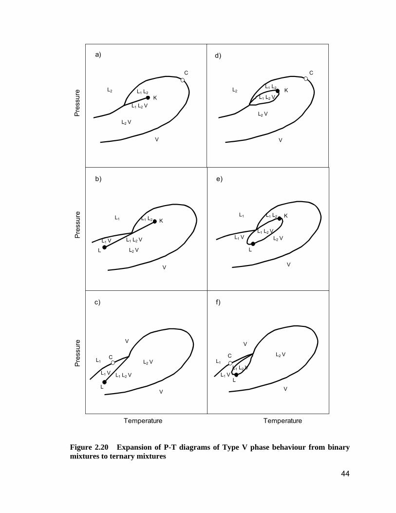
44
Figure 2.20 Expansion of P-T diagrams of Type V phase behaviour from binary mixtures to ternary mixtures
a) d)
b) e)
Temperature Temperature
Pre
ssur
eP
ress
ure
c) f)
L1 L2 V
V
L1 L2
L2 V
L2
L1 L2 V
V
L1 L2
L2 V
L1
L1 V
K
K
L
L1 L2 V
V
L2 VL1
L1 V
V
L
C
CP
ress
ure
L1 L2
L2 V
L2
C
V
L1 L2 VK
L1 L2 V
V
L1 L2
L2 V
L1
L1 L2 VL1 V
K
L
V
L2 V
L
C
L1 L2 VL1 V
L1
V
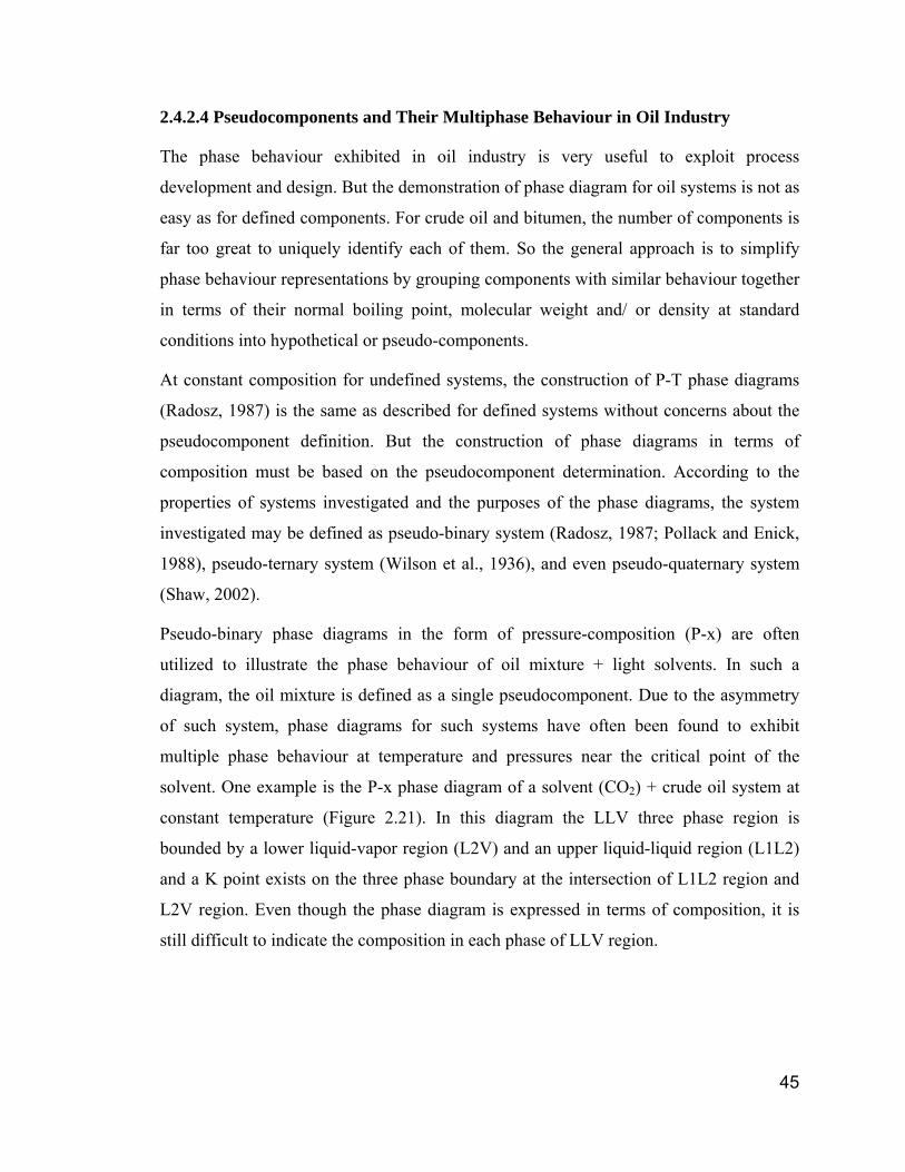
45
2.4.2.4 Pseudocomponents and Their Multiphase Behaviour in Oil Industry
The phase behaviour exhibited in oil industry is very useful to exploit process
development and design. But the demonstration of phase diagram for oil systems is not as
easy as for defined components. For crude oil and bitumen, the number of components is
far too great to uniquely identify each of them. So the general approach is to simplify
phase behaviour representations by grouping components with similar behaviour together
in terms of their normal boiling point, molecular weight and/ or density at standard
conditions into hypothetical or pseudo-components.
At constant composition for undefined systems, the construction of P-T phase diagrams
(Radosz, 1987) is the same as described for defined systems without concerns about the
pseudocomponent definition. But the construction of phase diagrams in terms of
composition must be based on the pseudocomponent determination. According to the
properties of systems investigated and the purposes of the phase diagrams, the system
investigated may be defined as pseudo-binary system (Radosz, 1987; Pollack and Enick,
1988), pseudo-ternary system (Wilson et al., 1936), and even pseudo-quaternary system
(Shaw, 2002).
Pseudo-binary phase diagrams in the form of pressure-composition (P-x) are often
utilized to illustrate the phase behaviour of oil mixture + light solvents. In such a
diagram, the oil mixture is defined as a single pseudocomponent. Due to the asymmetry
of such system, phase diagrams for such systems have often been found to exhibit
multiple phase behaviour at temperature and pressures near the critical point of the
solvent. One example is the P-x phase diagram of a solvent (CO2) + crude oil system at
constant temperature (Figure 2.21). In this diagram the LLV three phase region is
bounded by a lower liquid-vapor region (L2V) and an upper liquid-liquid region (L1L2)
and a K point exists on the three phase boundary at the intersection of L1L2 region and
L2V region. Even though the phase diagram is expressed in terms of composition, it is
still difficult to indicate the composition in each phase of LLV region.
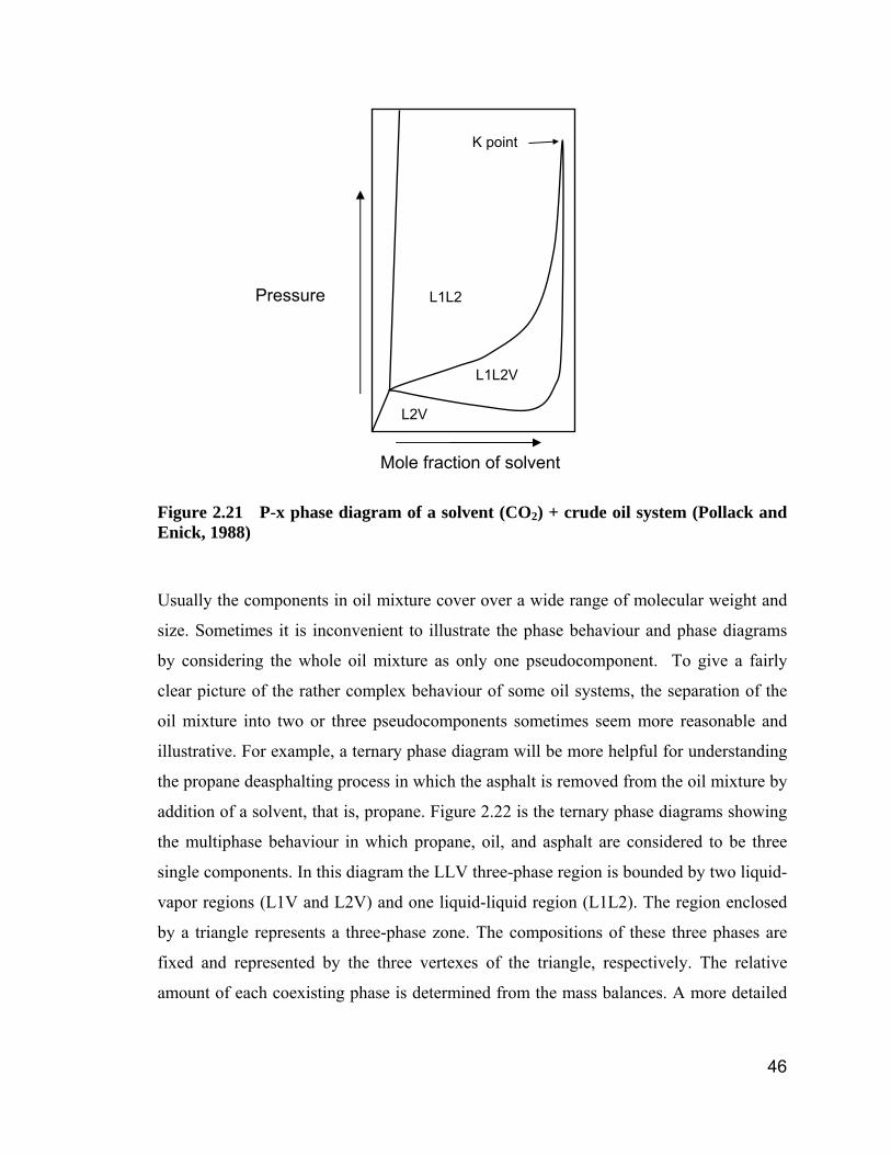
46
Figure 2.21 P-x phase diagram of a solvent (CO2) + crude oil system (Pollack and Enick, 1988)
Usually the components in oil mixture cover over a wide range of molecular weight and
size. Sometimes it is inconvenient to illustrate the phase behaviour and phase diagrams
by considering the whole oil mixture as only one pseudocomponent. To give a fairly
clear picture of the rather complex behaviour of some oil systems, the separation of the
oil mixture into two or three pseudocomponents sometimes seem more reasonable and
illustrative. For example, a ternary phase diagram will be more helpful for understanding
the propane deasphalting process in which the asphalt is removed from the oil mixture by
addition of a solvent, that is, propane. Figure 2.22 is the ternary phase diagrams showing
the multiphase behaviour in which propane, oil, and asphalt are considered to be three
single components. In this diagram the LLV three-phase region is bounded by two liquid-
vapor regions (L1V and L2V) and one liquid-liquid region (L1L2). The region enclosed
by a triangle represents a three-phase zone. The compositions of these three phases are
fixed and represented by the three vertexes of the triangle, respectively. The relative
amount of each coexisting phase is determined from the mass balances. A more detailed
Mole fraction of solvent
Pressure L1L2
K point
L2V
L1L2V
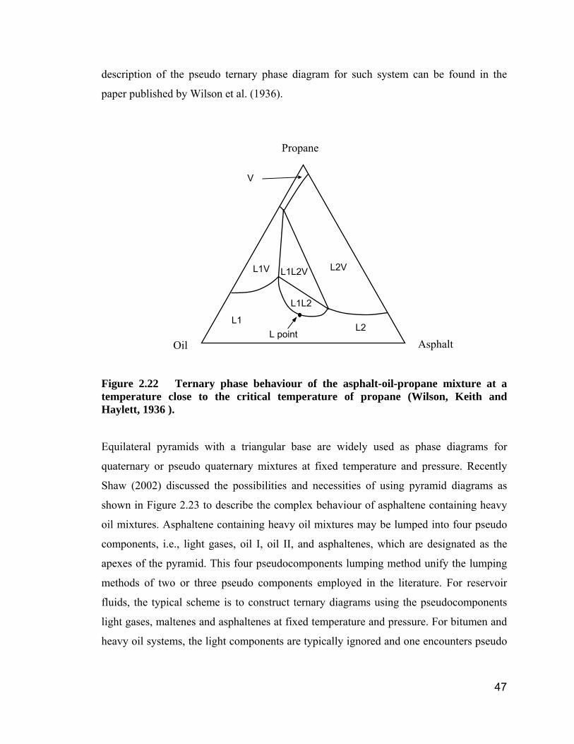
47
description of the pseudo ternary phase diagram for such system can be found in the
paper published by Wilson et al. (1936).
Figure 2.22 Ternary phase behaviour of the asphalt-oil-propane mixture at a temperature close to the critical temperature of propane (Wilson, Keith and Haylett, 1936 ).
Equilateral pyramids with a triangular base are widely used as phase diagrams for
quaternary or pseudo quaternary mixtures at fixed temperature and pressure. Recently
Shaw (2002) discussed the possibilities and necessities of using pyramid diagrams as
shown in Figure 2.23 to describe the complex behaviour of asphaltene containing heavy
oil mixtures. Asphaltene containing heavy oil mixtures may be lumped into four pseudo
components, i.e., light gases, oil I, oil II, and asphaltenes, which are designated as the
apexes of the pyramid. This four pseudocomponents lumping method unify the lumping
methods of two or three pseudo components employed in the literature. For reservoir
fluids, the typical scheme is to construct ternary diagrams using the pseudocomponents
light gases, maltenes and asphaltenes at fixed temperature and pressure. For bitumen and
heavy oil systems, the light components are typically ignored and one encounters pseudo
Propane
Oil Asphalt
L1L2V L2V
L1L2
L1V
L1 L2
V
L point
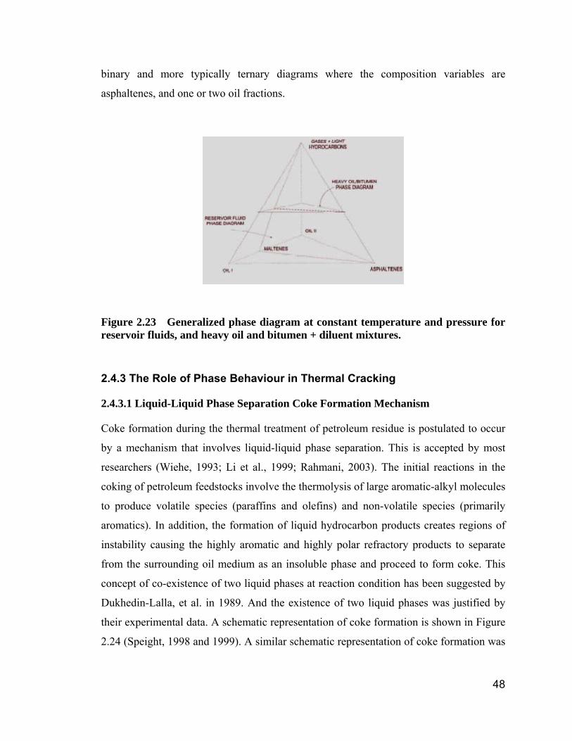
48
binary and more typically ternary diagrams where the composition variables are
asphaltenes, and one or two oil fractions.
Figure 2.23 Generalized phase diagram at constant temperature and pressure for reservoir fluids, and heavy oil and bitumen + diluent mixtures.
2.4.3 The Role of Phase Behaviour in Thermal Cracking
2.4.3.1 Liquid-Liquid Phase Separation Coke Formation Mechanism
Coke formation during the thermal treatment of petroleum residue is postulated to occur
by a mechanism that involves liquid-liquid phase separation. This is accepted by most
researchers (Wiehe, 1993; Li et al., 1999; Rahmani, 2003). The initial reactions in the
coking of petroleum feedstocks involve the thermolysis of large aromatic-alkyl molecules
to produce volatile species (paraffins and olefins) and non-volatile species (primarily
aromatics). In addition, the formation of liquid hydrocarbon products creates regions of
instability causing the highly aromatic and highly polar refractory products to separate
from the surrounding oil medium as an insoluble phase and proceed to form coke. This
concept of co-existence of two liquid phases at reaction condition has been suggested by
Dukhedin-Lalla, et al. in 1989. And the existence of two liquid phases was justified by
their experimental data. A schematic representation of coke formation is shown in Figure
2.24 (Speight, 1998 and 1999). A similar schematic representation of coke formation was
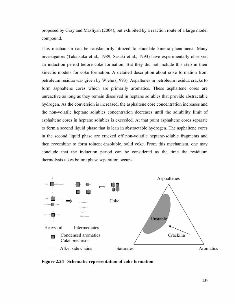
49
proposed by Gray and Masliyah (2004), but exhibited by a reaction route of a large model
compound.
This mechanism can be satisfactorily utilized to elucidate kinetic phenomena. Many
investigators (Takatsuka et al., 1989; Sasaki et al., 1993) have experimentally observed
an induction period before coke formation. But they did not include this step in their
kinectic models for coke formation. A detailed description about coke formation from
petroleum residua was given by Wiehe (1993). Aspaltenes in petroleum residua cracks to
form asphaltene cores which are primarily aromatics. These asphaltene cores are
unreactive as long as they remain dissolved in heptane solubles that provide abstractable
hydrogen. As the conversion is increased, the asphaltene core concentration increases and
the non-volatile heptane solubles concentration decreases until the solubility limit of
asphaltene cores in heptane solubles is exceeded. At that point asphaltene cores separate
to form a second liquid phase that is lean in abstractable hydrogen. The asphaltene cores
in the second liquid phase are cracked off non-volatile heptane-soluble fragments and
then recombine to form toluene-insoluble, solid coke. From this mechanism, one may
conclude that the induction period can be considered as the time the residuum
thermolysis takes before phase separation occurs.
Figure 2.24 Schematic representation of coke formation
Heavy oil Intermediates
Coke
Condensed aromatics Coke precursor
Alkyl side chains
Asphaltenes
Saturates Aromatics
Unstable
Cracking
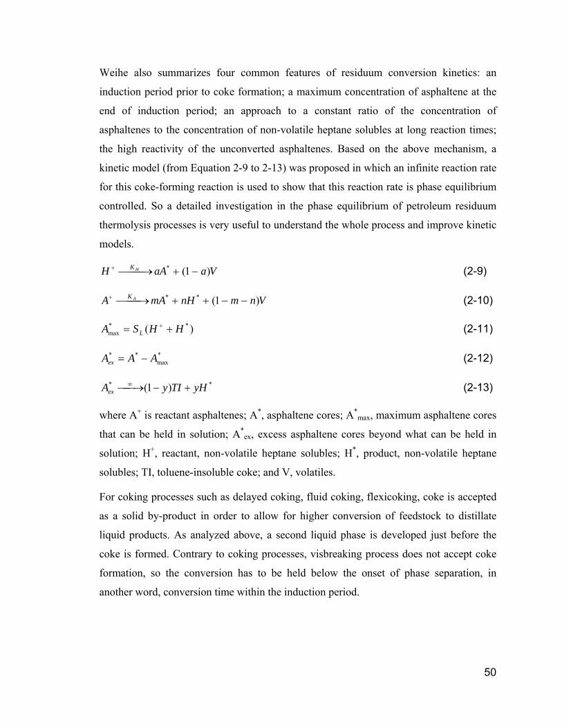
50
Weihe also summarizes four common features of residuum conversion kinetics: an
induction period prior to coke formation; a maximum concentration of asphaltene at the
end of induction period; an approach to a constant ratio of the concentration of
asphaltenes to the concentration of non-volatile heptane solubles at long reaction times;
the high reactivity of the unconverted asphaltenes. Based on the above mechanism, a
kinetic model (from Equation 2-9 to 2-13) was proposed in which an infinite reaction rate
for this coke-forming reaction is used to show that this reaction rate is phase equilibrium
controlled. So a detailed investigation in the phase equilibrium of petroleum residuum
thermolysis processes is very useful to understand the whole process and improve kinetic
models.
VaaAH HK )1(* −+⎯⎯→⎯+ (2-9)
VnmnHmAA AK )1(** −−++⎯⎯→⎯+ (2-10)
)( **max HHSA L += + (2-11)
*max
** AAAex −= (2-12)
** )1( yHTIyAex +−⎯→⎯∞ (2-13)
where A+ is reactant asphaltenes; A*, asphaltene cores; A*max, maximum asphaltene cores
that can be held in solution; A*ex, excess asphaltene cores beyond what can be held in
solution; H+, reactant, non-volatile heptane solubles; H*, product, non-volatile heptane
solubles; TI, toluene-insoluble coke; and V, volatiles.
For coking processes such as delayed coking, fluid coking, flexicoking, coke is accepted
as a solid by-product in order to allow for higher conversion of feedstock to distillate
liquid products. As analyzed above, a second liquid phase is developed just before the
coke is formed. Contrary to coking processes, visbreaking process does not accept coke
formation, so the conversion has to be held below the onset of phase separation, in
another word, conversion time within the induction period.
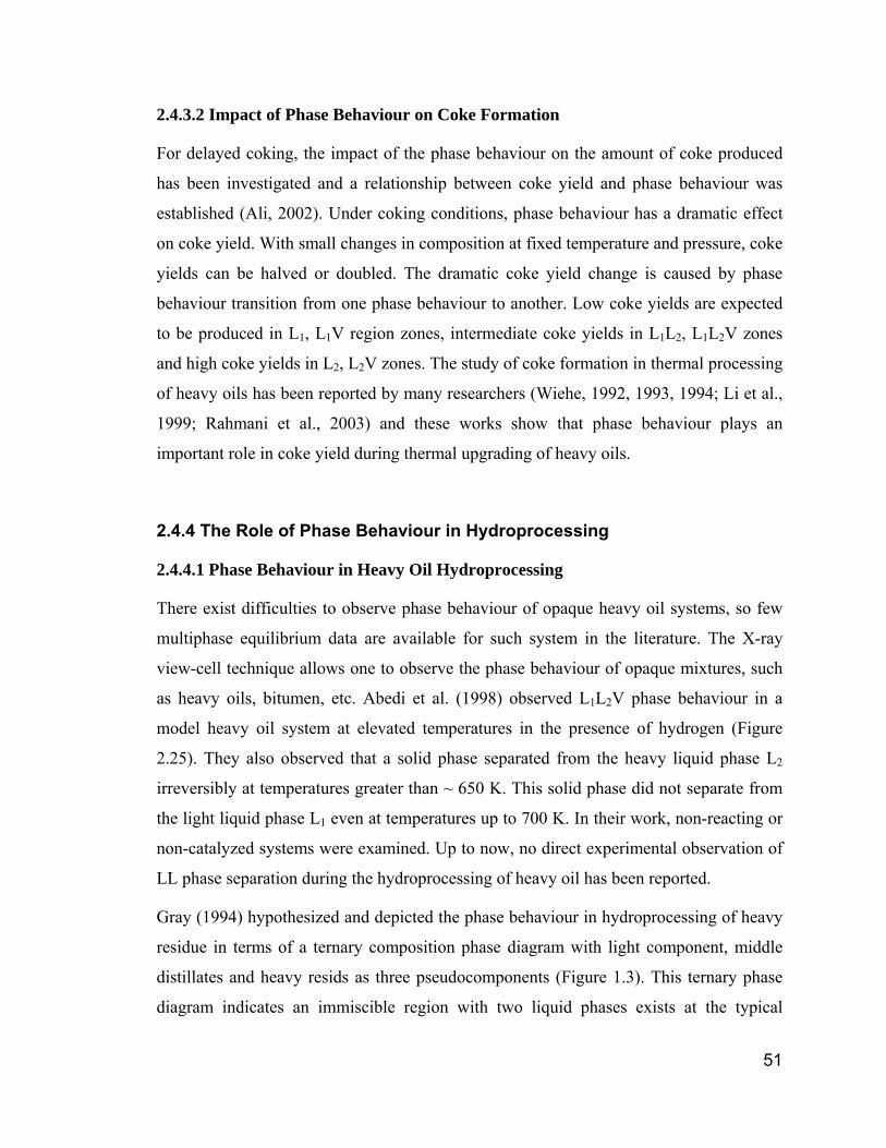
51
2.4.3.2 Impact of Phase Behaviour on Coke Formation
For delayed coking, the impact of the phase behaviour on the amount of coke produced
has been investigated and a relationship between coke yield and phase behaviour was
established (Ali, 2002). Under coking conditions, phase behaviour has a dramatic effect
on coke yield. With small changes in composition at fixed temperature and pressure, coke
yields can be halved or doubled. The dramatic coke yield change is caused by phase
behaviour transition from one phase behaviour to another. Low coke yields are expected
to be produced in L1, L1V region zones, intermediate coke yields in L1L2, L1L2V zones
and high coke yields in L2, L2V zones. The study of coke formation in thermal processing
of heavy oils has been reported by many researchers (Wiehe, 1992, 1993, 1994; Li et al.,
1999; Rahmani et al., 2003) and these works show that phase behaviour plays an
important role in coke yield during thermal upgrading of heavy oils.
2.4.4 The Role of Phase Behaviour in Hydroprocessing
2.4.4.1 Phase Behaviour in Heavy Oil Hydroprocessing
There exist difficulties to observe phase behaviour of opaque heavy oil systems, so few
multiphase equilibrium data are available for such system in the literature. The X-ray
view-cell technique allows one to observe the phase behaviour of opaque mixtures, such
as heavy oils, bitumen, etc. Abedi et al. (1998) observed L1L2V phase behaviour in a
model heavy oil system at elevated temperatures in the presence of hydrogen (Figure
2.25). They also observed that a solid phase separated from the heavy liquid phase L2
irreversibly at temperatures greater than ~ 650 K. This solid phase did not separate from
the light liquid phase L1 even at temperatures up to 700 K. In their work, non-reacting or
non-catalyzed systems were examined. Up to now, no direct experimental observation of
LL phase separation during the hydroprocessing of heavy oil has been reported.
Gray (1994) hypothesized and depicted the phase behaviour in hydroprocessing of heavy
residue in terms of a ternary composition phase diagram with light component, middle
distillates and heavy resids as three pseudocomponents (Figure 1.3). This ternary phase
diagram indicates an immiscible region with two liquid phases exists at the typical
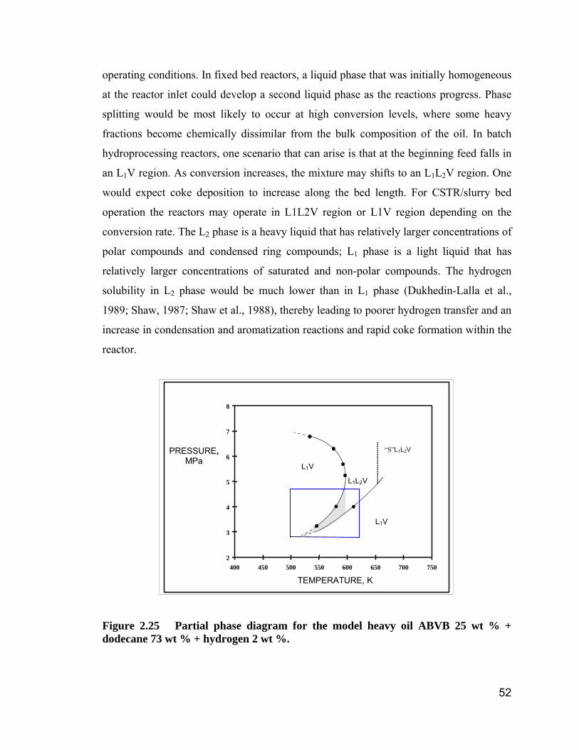
52
operating conditions. In fixed bed reactors, a liquid phase that was initially homogeneous
at the reactor inlet could develop a second liquid phase as the reactions progress. Phase
splitting would be most likely to occur at high conversion levels, where some heavy
fractions become chemically dissimilar from the bulk composition of the oil. In batch
hydroprocessing reactors, one scenario that can arise is that at the beginning feed falls in
an L1V region. As conversion increases, the mixture may shifts to an L1L2V region. One
would expect coke deposition to increase along the bed length. For CSTR/slurry bed
operation the reactors may operate in L1L2V region or L1V region depending on the
conversion rate. The L2 phase is a heavy liquid that has relatively larger concentrations of
polar compounds and condensed ring compounds; L1 phase is a light liquid that has
relatively larger concentrations of saturated and non-polar compounds. The hydrogen
solubility in L2 phase would be much lower than in L1 phase (Dukhedin-Lalla et al.,
1989; Shaw, 1987; Shaw et al., 1988), thereby leading to poorer hydrogen transfer and an
increase in condensation and aromatization reactions and rapid coke formation within the
reactor.
Figure 2.25 Partial phase diagram for the model heavy oil ABVB 25 wt % + dodecane 73 wt % + hydrogen 2 wt %.
2
3
4
5
6
7
8
400 450 500 550 600 650 700 750
TEMPERATURE, K
PRESSURE, MPa
“S”L1L2V
L1V
L1V
L1L2V
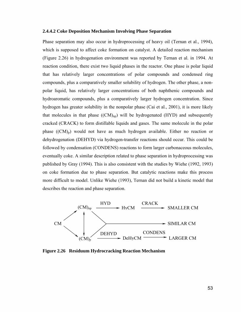
53
2.4.4.2 Coke Deposition Mechanism Involving Phase Separation
Phase separation may also occur in hydroprocessing of heavy oil (Ternan et al., 1994),
which is supposed to affect coke formation on catalyst. A detailed reaction mechanism
(Figure 2.26) in hydrogenation environment was reported by Ternan et al. in 1994. At
reaction condition, there exist two liquid phases in the reactor. One phase is polar liquid
that has relatively larger concentrations of polar compounds and condensed ring
compounds, plus a comparatively smaller solubility of hydrogen. The other phase, a non-
polar liquid, has relatively larger concentrations of both naphthenic compounds and
hydroaromatic compounds, plus a comparatively larger hydrogen concentration. Since
hydrogen has greater solubility in the nonpolar phase (Cai et al., 2001), it is more likely
that molecules in that phase ((CM)np) will be hydrogenated (HYD) and subsequently
cracked (CRACK) to form distillable liquids and gases. The same molecule in the polar
phase ((CM)p) would not have as much hydrogen available. Either no reaction or
dehydrogenation (DEHYD) via hydrogen-transfer reactions should occur. This could be
followed by condensation (CONDENS) reactions to form larger carbonaceous molecules,
eventually coke. A similar description related to phase separation in hydroprocessing was
published by Gray (1994). This is also consistent with the studies by Wiehe (1992, 1993)
on coke formation due to phase separation. But catalytic reactions make this process
more difficult to model. Unlike Wiehe (1993), Ternan did not build a kinetic model that
describes the reaction and phase separation.
Figure 2.26 Residuum Hydrocracking Reaction Mechanism
CM
(CM)np
(CM)p
HyCM
DeHyCM
HYD
DEHYD
SMALLER CMCRACK
CONDENSLARGER CM
SIMILAR CM
54
2.4.5 Coke Formation Mechanism Involving Colloidal Phenomena
As discussed above, the phase separation is caused by asphaltenes exceeding the
solubility limit of the oil as reactions proceed, while the formation of asphaltene rich
phases discussed by Storm et al. (1995; 1996; 1998) is purely physical – flocculation and
precipitation. It has been concluded that heavy oils such as crude oils, residues, bitumen
etc. exhibit colloidal behaviour in the presence of asphaltenes, and resin fractions (Li et
al. 1996; Bardon et al. 1996; Branco et al. 2001). The asphaltenes are believed to exist in
heavy oils partly dissolved and partly in steric-colloidal and/or micellar forms depending
on the polarity of their oil medium and presence of other compounds (Priyanto et al.
2001). But asphaltenes and heavier species can precipitate from the oil matrix if the
colloid stability of the feed cannot be maintained. Storm et al. (1995; 1996; 1998)
observed that asphaltenes could flocculate and precipitate to form another asphaltenic
phase at elevated temperature even well below the temperature at which chemical
reactions occur. They suggested that the asphaltenic phase is the precursor to the coke-
producing phase in the reacting residue. Under catalytic hydroprocessing conditions, this
colloidal structure is more likely disrupted and asphaltenes and heavier species can
precipitate on the catalyst surface because of instabilities caused by thermal and
hydrogenation reactions, which may enhance coke formation (Furimsky and Massoth,
1999). The incompatibility is partly due to the competing thermal and catalytic reactions,
but mainly due to the difference in the reactivity of the components of the residual oil,
namely, oils, resins, and asphaltens (Matsushita et al. 2004). Under such conditions, the
naphthenic groups and alkyl side chains in the asphaltene molecules will be cracked off.
The remaining polynuclear aromatic core of the asphaltene molecules will be less soluble
in the oil medium since the resins, which act as a solubilizing agent, are also
hydrogenated and cracked in the process. The cracking rate of resins is faster than the
asphaltenes. All of these cause the asphaltenes sedimentation, which enhances coke
deposition on the catalyst. The instability of hydrotreated heavy oil products was recently
proved using a flocculation onset titration method (Bartholdy et al. 2000; 2001).
55
2.5 Summary
With the depletion of conventional crude oils, the rocketing rise of petroleum price, and
more and more stringent environmental regulations, refiners must convert the "bottom of
barrel" into "light, clean fuels". Consequently, heavy oil hydroprocessing plays an
increasingly key role as a primary upgrading process. Diverse processes are in industrial
use or nearing commercialization. In all cases, catalyst fouling is a major concern.
Considerable effort has been devoted to this research area. Although significant progress
has been made, many issues are still debated in the literature. There is no general
agreement on coke deposition modes, coke deposition mechanisms and related issues
from industrial perspectives and more effort needs to be devoted to the study of coke
deposition. Some observed phenomena such as irregular coke deposition profiles, coke
suppression by addition of solvents, indicate that phase behaviour may be an important
factor influencing coke deposition. But many of the following questions regarding this
area have not been answered in the literature. Does a second liquid phase exist or develop
under typical hydroprocessing conditions and does resid conversion extent affect the
nature of the phase behaviour? What is the impact of phase behaviour on coke deposition
both with respect to coke content and coke deposition modes? How does phase behaviour
affect coke deposition through the significant difference in properties of the co-existing
phases? Due to prior experimental technique limitations, there is no direct proof of the
role played by phase behaviour in the literature. The experimental technique employed in
this study and the planned experiments are expected to provide significant insights into
the research on coke deposition in catalytic heavy oil hydroprocessing.
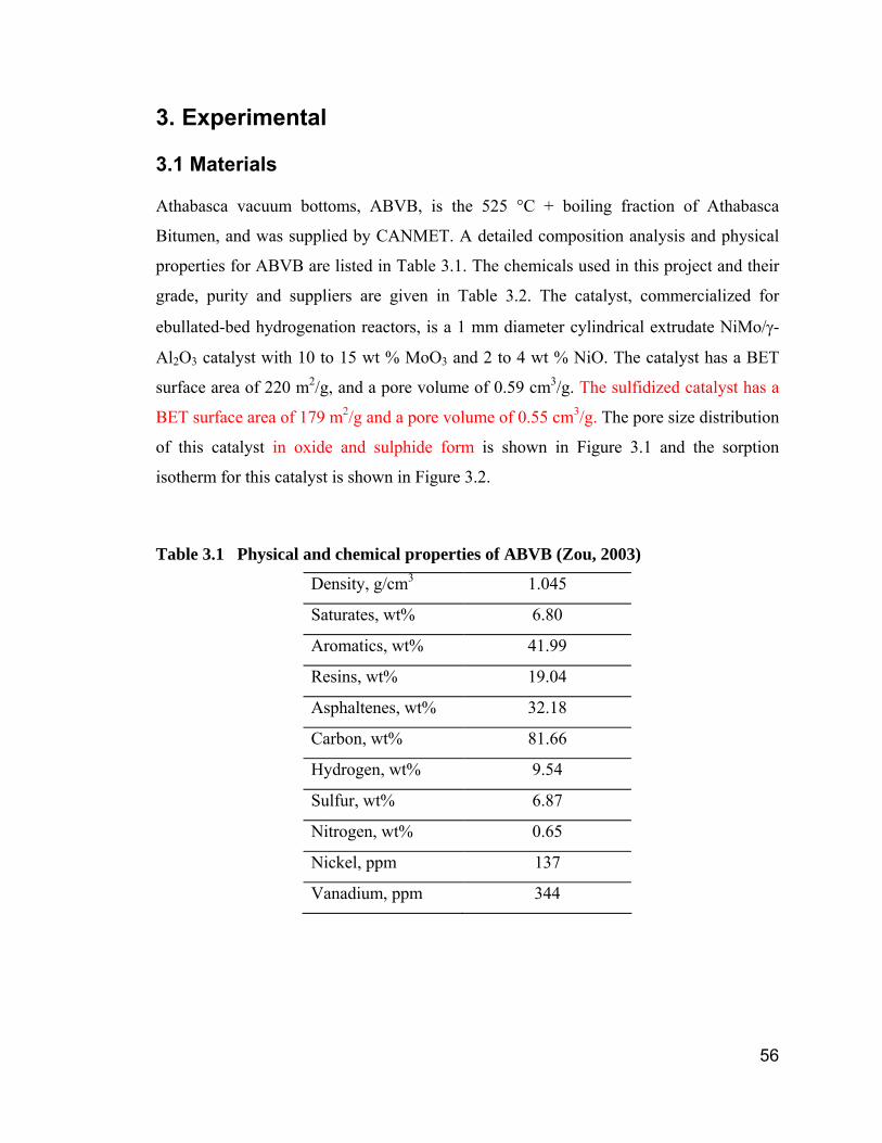
56
3. Experimental
3.1 Materials
Athabasca vacuum bottoms, ABVB, is the 525 °C + boiling fraction of Athabasca
Bitumen, and was supplied by CANMET. A detailed composition analysis and physical
properties for ABVB are listed in Table 3.1. The chemicals used in this project and their
grade, purity and suppliers are given in Table 3.2. The catalyst, commercialized for
ebullated-bed hydrogenation reactors, is a 1 mm diameter cylindrical extrudate NiMo/γ-
Al2O3 catalyst with 10 to 15 wt % MoO3 and 2 to 4 wt % NiO. The catalyst has a BET
surface area of 220 m2/g, and a pore volume of 0.59 cm3/g. The sulfidized catalyst has a
BET surface area of 179 m2/g and a pore volume of 0.55 cm3/g. The pore size distribution
of this catalyst in oxide and sulphide form is shown in Figure 3.1 and the sorption
isotherm for this catalyst is shown in Figure 3.2.
Table 3.1 Physical and chemical properties of ABVB (Zou, 2003)
Density, g/cm3 1.045
Saturates, wt% 6.80
Aromatics, wt% 41.99
Resins, wt% 19.04
Asphaltenes, wt% 32.18
Carbon, wt% 81.66
Hydrogen, wt% 9.54
Sulfur, wt% 6.87
Nitrogen, wt% 0.65
Nickel, ppm 137
Vanadium, ppm 344
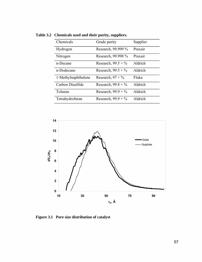
57
Table 3.2 Chemicals used and their purity, suppliers.
Chemicals Grade purity Supplier
Hydrogen Research, 99.999 % Praxair
Nitrogen Research, 99.998 % Praxair
n-Decane Research, 99.5 + % Aldrich
n-Dodecane Research, 99.5 + % Aldrich
1-Methylnaphthalene Research, 97 + % Fluka
Carbon Disulfide Research, 99.8 + % Aldrich
Toluene Research, 99.9 + % Aldrich
Tetrahydrofuran Research, 99.9 + % Aldrich
0
2
4
6
8
10
12
14
10 30 50 70 90
rp, Ǻ
dVp/
drp
Oxide
Sulphide
Figure 3.1 Pore size distribution of catalyst
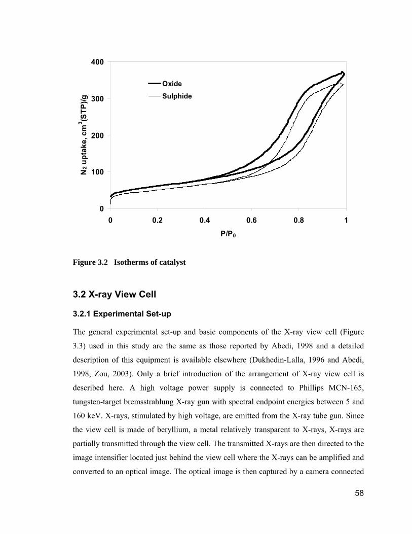
58
0
100
200
300
400
0 0.2 0.4 0.6 0.8 1
P/P0
N2 u
ptak
e, c
m3 (S
TP)/g
Oxide
Sulphide
Figure 3.2 Isotherms of catalyst
3.2 X-ray View Cell
3.2.1 Experimental Set-up
The general experimental set-up and basic components of the X-ray view cell (Figure
3.3) used in this study are the same as those reported by Abedi, 1998 and a detailed
description of this equipment is available elsewhere (Dukhedin-Lalla, 1996 and Abedi,
1998, Zou, 2003). Only a brief introduction of the arrangement of X-ray view cell is
described here. A high voltage power supply is connected to Phillips MCN-165,
tungsten-target bremsstrahlung X-ray gun with spectral endpoint energies between 5 and
160 keV. X-rays, stimulated by high voltage, are emitted from the X-ray tube gun. Since
the view cell is made of beryllium, a metal relatively transparent to X-rays, X-rays are
partially transmitted through the view cell. The transmitted X-rays are then directed to the
image intensifier located just behind the view cell where the X-rays can be amplified and
converted to an optical image. The optical image is then captured by a camera connected
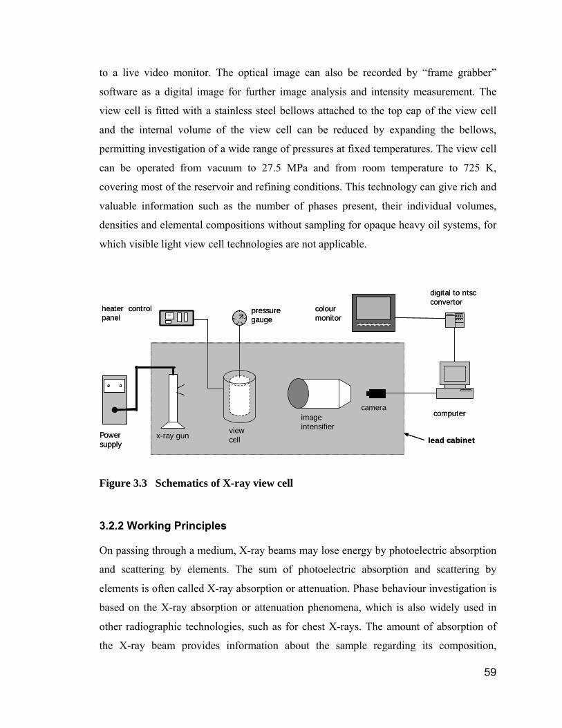
59
to a live video monitor. The optical image can also be recorded by “frame grabber”
software as a digital image for further image analysis and intensity measurement. The
view cell is fitted with a stainless steel bellows attached to the top cap of the view cell
and the internal volume of the view cell can be reduced by expanding the bellows,
permitting investigation of a wide range of pressures at fixed temperatures. The view cell
can be operated from vacuum to 27.5 MPa and from room temperature to 725 K,
covering most of the reservoir and refining conditions. This technology can give rich and
valuable information such as the number of phases present, their individual volumes,
densities and elemental compositions without sampling for opaque heavy oil systems, for
which visible light view cell technologies are not applicable.
1000PSIG
77 F
camera
colour monitor
heater control panel
pressuregauge
viewcell
image intensifier
x-ray gunPower supply
computer
digital to ntscconvertor
lead cabinet
1000PSIG
77 F
camera
colour monitor
heater control panel
pressuregauge
viewcell
image intensifier
x-ray gunPower supply
computer
digital to ntscconvertor
lead cabinet
Figure 3.3 Schematics of X-ray view cell
3.2.2 Working Principles
On passing through a medium, X-ray beams may lose energy by photoelectric absorption
and scattering by elements. The sum of photoelectric absorption and scattering by
elements is often called X-ray absorption or attenuation. Phase behaviour investigation is
based on the X-ray absorption or attenuation phenomena, which is also widely used in
other radiographic technologies, such as for chest X-rays. The amount of absorption of
the X-ray beam provides information about the sample regarding its composition,
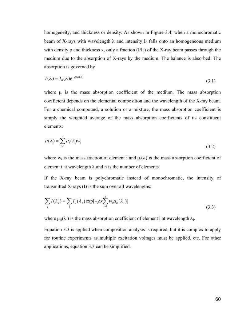
60
homogeneity, and thickness or density. As shown in Figure 3.4, when a monochromatic
beam of X-rays with wavelength λ and intensity I0 falls onto an homogeneous medium
with density ρ and thickness x, only a fraction (I/I0) of the X-ray beam passes through the
medium due to the absorption of X-rays by the medium. The balance is absorbed. The
absorption is governed by
)(0 )()( λμρλλ xeII −= (3.1)
where μ is the mass absorption coefficient of the medium. The mass absorption
coefficient depends on the elemental composition and the wavelength of the X-ray beam.
For a chemical compound, a solution or a mixture, the mass absorption coefficient is
simply the weighted average of the mass absorption coefficients of its constituent
elements:
∑=
=n
iii w
1
)()( λμλμ (3.2)
where wi is the mass fraction of element i and μi(λ) is the mass absorption coefficient of
element i at wavelength λ and n is the number of elements.
If the X-ray beam is polychromatic instead of monochromatic, the intensity of
transmitted X-rays (I) is the sum over all wavelengths:
∑∑∑=
−=n
ijiji
jj
jj wxII
10 )](exp[)()( λμρλλ
(3.3)
where μij(λj) is the mass absorption coefficient of element i at wavelength λj.
Equation 3.3 is applied when composition analysis is required, but it is complex to apply
for routine experiments as multiple excitation voltages must be applied, etc. For other
applications, equation 3.3 can be simplified.
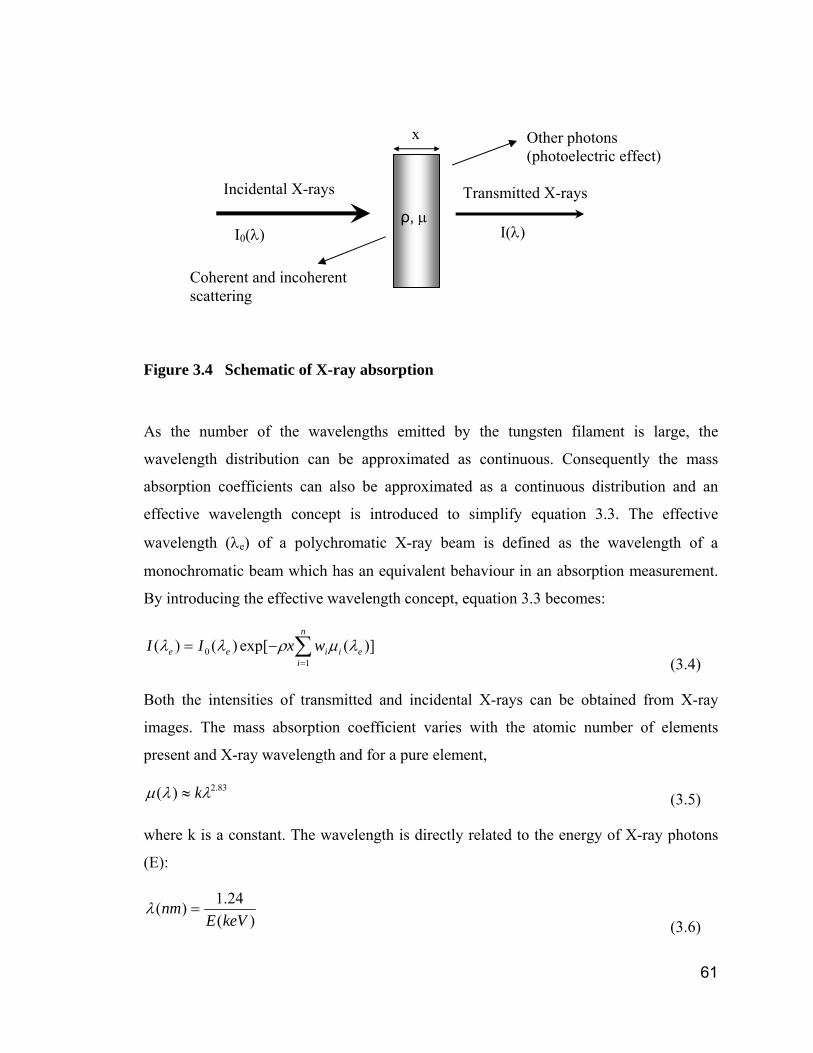
61
Figure 3.4 Schematic of X-ray absorption
As the number of the wavelengths emitted by the tungsten filament is large, the
wavelength distribution can be approximated as continuous. Consequently the mass
absorption coefficients can also be approximated as a continuous distribution and an
effective wavelength concept is introduced to simplify equation 3.3. The effective
wavelength (λe) of a polychromatic X-ray beam is defined as the wavelength of a
monochromatic beam which has an equivalent behaviour in an absorption measurement.
By introducing the effective wavelength concept, equation 3.3 becomes:
∑=
−=n
ieiiee wxII
10 )](exp[)()( λμρλλ
(3.4)
Both the intensities of transmitted and incidental X-rays can be obtained from X-ray
images. The mass absorption coefficient varies with the atomic number of elements
present and X-ray wavelength and for a pure element,
83.2)( λλμ k≈ (3.5)
where k is a constant. The wavelength is directly related to the energy of X-ray photons
(E):
)(24.1)(
keVEnm =λ
(3.6)
x
Incidental X-rays
I(λ)
Other photons (photoelectric effect)
Coherent and incoherent scattering
I0(λ)
Transmitted X-rays ρ, μ
62
Experimental absorption coefficient data can be found in literature (de Bore, 1989). The
unknowns in equation 3.4 are density and elemental composition, which could be
obtained if transmitted X-ray images at different excitation conditions are available.
In this study, the elemental composition of each phase is not obtainable due to X-ray
scattering by asphaltene particles (Zou, 2003). Only an apparent fluid density is obtained.
A detailed deconvolution procedure for transmitted X-ray images used to calculate the
apparent density is presented in Zou’s thesis (2003). The same procedure is applied in
this study. The accuracy of density measurement for light hydrocarbons is ±12 kg/m3.
The phase volumes can be simply obtained by determining the interface heights and
bellows positions with the aid of a cell volume calibration. Volume calibration is taken
from Zou’s thesis (2003). The minimum detectable volume is 0.61 ml and the minimum
detectable volume difference is 0.12 ml - equivalent to the height of one pixel.
3.2.3 Illustration of a Single X-ray Transmission Image
From equation 3.1, the intensity of an X-ray transmission video image decreases
exponentially with density. Higher density materials appear darker since more X-rays are
absorbed or scattered, while lower density materials appear lighter since more X-rays
pass through. Figure 3.5 is an example of X-ray transmission image. This single image
was recorded at 360 °C and 24.26 bar for the 10% ABVB + decane mixture. Based on
visual observation, this image shows LLV phase behaviour. In this image, the bellows is
pulled back to the top of the view cell. The lower density liquid phase (L1) is represented
by the middle grey area. The vapour phase, represented by the light grey area, is above,
and the higher density liquid phase (L2), represented by the darker area, is below. From
images like this, it is easy to discern the existence of separate phases, the relative amount
of each phase, and the direction a phase boundary moves with changing process
conditions. This real-time, qualitative information is useful when attempting to determine
the type of phase behaviour a system exhibits. One can also process the images to provide
the quantitative information of a system, such as phase volume, and density. The intensity
and density profiles for the image shown in Figure 3.5 are shown in Figure 3.6. Even
though the intensity profile is not flat across a single phase, the density profile after
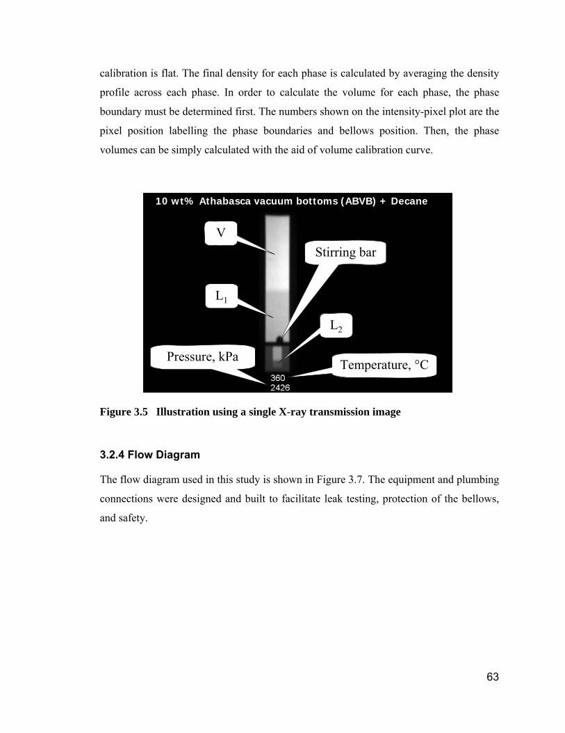
63
calibration is flat. The final density for each phase is calculated by averaging the density
profile across each phase. In order to calculate the volume for each phase, the phase
boundary must be determined first. The numbers shown on the intensity-pixel plot are the
pixel position labelling the phase boundaries and bellows position. Then, the phase
volumes can be simply calculated with the aid of volume calibration curve.
Stirring bar
L2
L1
V
Pressure, kPa Temperature, °C
10 wt% Athabasca vacuum bottoms (ABVB) + Decane
Stirring bar
L2
L1
V
Pressure, kPa Temperature, °C
10 wt% Athabasca vacuum bottoms (ABVB) + Decane
Figure 3.5 Illustration using a single X-ray transmission image
3.2.4 Flow Diagram
The flow diagram used in this study is shown in Figure 3.7. The equipment and plumbing
connections were designed and built to facilitate leak testing, protection of the bellows,
and safety.
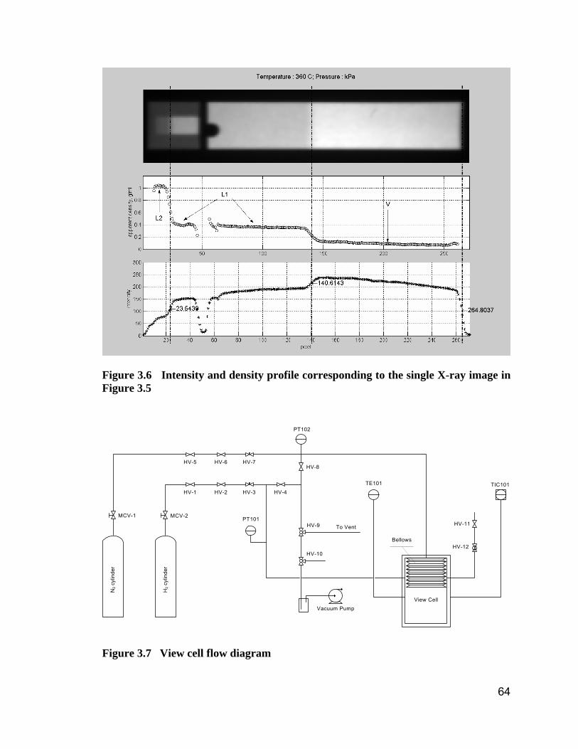
64
Figure 3.6 Intensity and density profile corresponding to the single X-ray image in Figure 3.5
MCV-1 MCV-2
HV-5 HV-6
HV-1 HV-2
Vacuum Pump
HV-4
HV-8
HV-11
HV-7
HV-3
HV-9
HV-12
PT102
PT101
TE101 TIC101
N2 c
ylin
der
H2 c
ylin
der
HV-10
To Vent
View Cell
Bellows
Figure 3.7 View cell flow diagram
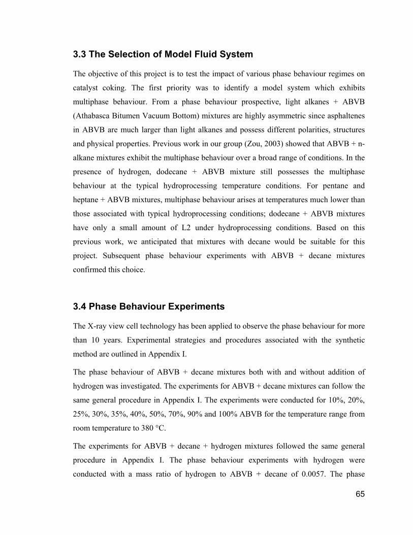
65
3.3 The Selection of Model Fluid System
The objective of this project is to test the impact of various phase behaviour regimes on
catalyst coking. The first priority was to identify a model system which exhibits
multiphase behaviour. From a phase behaviour prospective, light alkanes + ABVB
(Athabasca Bitumen Vacuum Bottom) mixtures are highly asymmetric since asphaltenes
in ABVB are much larger than light alkanes and possess different polarities, structures
and physical properties. Previous work in our group (Zou, 2003) showed that ABVB + n-
alkane mixtures exhibit the multiphase behaviour over a broad range of conditions. In the
presence of hydrogen, dodecane + ABVB mixture still possesses the multiphase
behaviour at the typical hydroprocessing temperature conditions. For pentane and
heptane + ABVB mixtures, multiphase behaviour arises at temperatures much lower than
those associated with typical hydroprocessing conditions; dodecane + ABVB mixtures
have only a small amount of L2 under hydroprocessing conditions. Based on this
previous work, we anticipated that mixtures with decane would be suitable for this
project. Subsequent phase behaviour experiments with ABVB + decane mixtures
confirmed this choice.
3.4 Phase Behaviour Experiments
The X-ray view cell technology has been applied to observe the phase behaviour for more
than 10 years. Experimental strategies and procedures associated with the synthetic
method are outlined in Appendix I.
The phase behaviour of ABVB + decane mixtures both with and without addition of
hydrogen was investigated. The experiments for ABVB + decane mixtures can follow the
same general procedure in Appendix I. The experiments were conducted for 10%, 20%,
25%, 30%, 35%, 40%, 50%, 70%, 90% and 100% ABVB for the temperature range from
room temperature to 380 °C.
The experiments for ABVB + decane + hydrogen mixtures followed the same general
procedure in Appendix I. The phase behaviour experiments with hydrogen were
conducted with a mass ratio of hydrogen to ABVB + decane of 0.0057. The phase
66
behaviour experiments with hydrogen case were conducted only for 10, 20, 30 and 40 wt
% ABVB.
At each examined condition, X-ray transmission images were recorded. Based on the
observation of a series of images and the systematic analysis of phase density and
volume, the phase diagrams were constructed. The image processing and data analysis
method was adopted from Zou, 2003 to calculate the densities, volumes of different
phases, but with modifications to the image processing and data analysis software. The
X-ray images and raw data from image analysis are summarized in Appendix II and
Appendix III respectively.
Since thermal cracking occurs at temperatures above 340 °C (Cai et al. 2001 a and b), the
samples were exposed to temperatures above 340 °C for less than one hour to avoid
significant cracking. Even so, phase diagrams at temperatures greater than 340 °C are
only approximate.
3.5 Catalyst Presulfidation
The catalyst presulfidation experiments were performed with 15-mL microbatch reactors
constructed from stainless-steel tubing and Swagelok fittings (Kanda et al. 2004). The
hydrogen and carbon disulfide amount, which is needed to presulfide the catalyst, is
calculated based on the following chemical reactions:
4222 24 CHSHHCS +=+ (3.7)
OHMoSHSHMoO 22223 32 +=++ (3.8)
OHSNiHSHNiO 22322 323 +=++ (3.9)
Prior to presulfidation, 350-mg catalyst was desiccated in an oven at 200 °C for 2 h. Then
the catalyst was transferred to a microbatch reactor, followed by injection of 70-μL liquid
carbon disulfide at room temperature, which is approximately twice the amount required
stoichiometrically to sulfidize the catalyst. After purging several times with hydrogen, the
sealed microbatch reactors were pressurized to 750 kPa, at room temperature, with
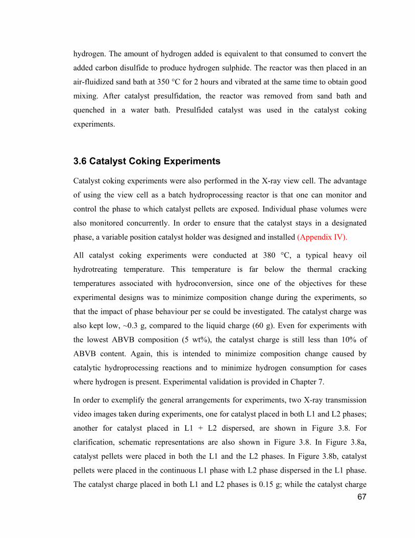
67
hydrogen. The amount of hydrogen added is equivalent to that consumed to convert the
added carbon disulfide to produce hydrogen sulphide. The reactor was then placed in an
air-fluidized sand bath at 350 °C for 2 hours and vibrated at the same time to obtain good
mixing. After catalyst presulfidation, the reactor was removed from sand bath and
quenched in a water bath. Presulfided catalyst was used in the catalyst coking
experiments.
3.6 Catalyst Coking Experiments
Catalyst coking experiments were also performed in the X-ray view cell. The advantage
of using the view cell as a batch hydroprocessing reactor is that one can monitor and
control the phase to which catalyst pellets are exposed. Individual phase volumes were
also monitored concurrently. In order to ensure that the catalyst stays in a designated
phase, a variable position catalyst holder was designed and installed (Appendix IV).
All catalyst coking experiments were conducted at 380 °C, a typical heavy oil
hydrotreating temperature. This temperature is far below the thermal cracking
temperatures associated with hydroconversion, since one of the objectives for these
experimental designs was to minimize composition change during the experiments, so
that the impact of phase behaviour per se could be investigated. The catalyst charge was
also kept low, ~0.3 g, compared to the liquid charge (60 g). Even for experiments with
the lowest ABVB composition (5 wt%), the catalyst charge is still less than 10% of
ABVB content. Again, this is intended to minimize composition change caused by
catalytic hydroprocessing reactions and to minimize hydrogen consumption for cases
where hydrogen is present. Experimental validation is provided in Chapter 7.
In order to exemplify the general arrangements for experiments, two X-ray transmission
video images taken during experiments, one for catalyst placed in both L1 and L2 phases;
another for catalyst placed in L1 + L2 dispersed, are shown in Figure 3.8. For
clarification, schematic representations are also shown in Figure 3.8. In Figure 3.8a,
catalyst pellets were placed in both the L1 and the L2 phases. In Figure 3.8b, catalyst
pellets were placed in the continuous L1 phase with L2 phase dispersed in the L1 phase.
The catalyst charge placed in both L1 and L2 phases is 0.15 g; while the catalyst charge
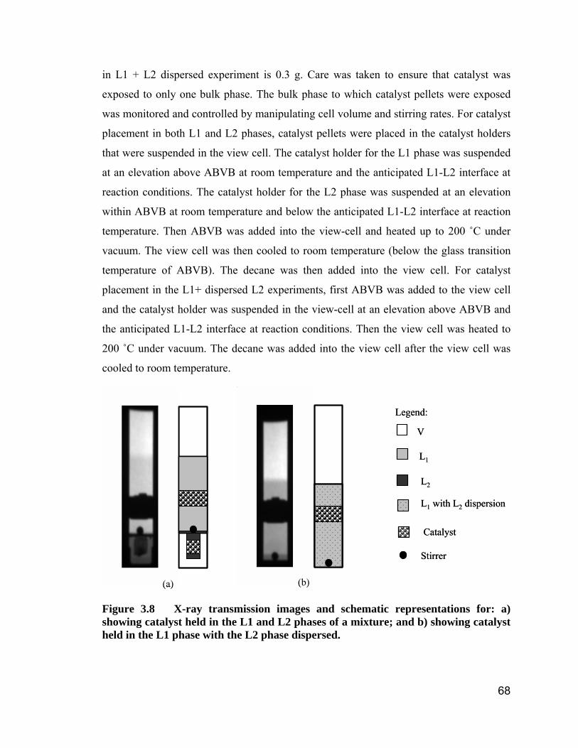
68
in L1 + L2 dispersed experiment is 0.3 g. Care was taken to ensure that catalyst was
exposed to only one bulk phase. The bulk phase to which catalyst pellets were exposed
was monitored and controlled by manipulating cell volume and stirring rates. For catalyst
placement in both L1 and L2 phases, catalyst pellets were placed in the catalyst holders
that were suspended in the view cell. The catalyst holder for the L1 phase was suspended
at an elevation above ABVB at room temperature and the anticipated L1-L2 interface at
reaction conditions. The catalyst holder for the L2 phase was suspended at an elevation
within ABVB at room temperature and below the anticipated L1-L2 interface at reaction
temperature. Then ABVB was added into the view-cell and heated up to 200 ˚C under
vacuum. The view cell was then cooled to room temperature (below the glass transition
temperature of ABVB). The decane was then added into the view cell. For catalyst
placement in the L1+ dispersed L2 experiments, first ABVB was added to the view cell
and the catalyst holder was suspended in the view-cell at an elevation above ABVB and
the anticipated L1-L2 interface at reaction conditions. Then the view cell was heated to
200 ˚C under vacuum. The decane was added into the view cell after the view cell was
cooled to room temperature.
V
L1
L2
L1 with L2 dispersion
Catalyst
Stirrer
Legend:
(a) (b)
V
L1
L2
L1 with L2 dispersion
Catalyst
Stirrer
Legend:
(a) (b)
Figure 3.8 X-ray transmission images and schematic representations for: a) showing catalyst held in the L1 and L2 phases of a mixture; and b) showing catalyst held in the L1 phase with the L2 phase dispersed.
69
The catalyst coking experiments both with and without hydrogen were performed. Once
the catalyst and all fluids were in place, the reactor was degassed under mild vacuum
(~30 kPa) for 30 minutes prior to heating. For the case with hydrogen, the view cell was
pressurized with hydrogen to a calculated pressure equivalent to 0.342 g of hydrogen.
The temperature profiles for heating, reaction, and cooling are shown in Figure 3.9. The
reaction times at 380 °C were 2 hours and 5 hours. As reaction rates are negligible at
temperatures below ~ 300 °C (Cai et al. 2001a, b), there is sufficient time, during the
three-hour heating period for diffusion processes to approach completion prior to the
occurrence of chemical reaction. At the end of an experiment, the reactor was cooled to
room temperature over a three-hour period.
3 hr 3 hr Reaction time
380°C Constant temperature reaction
Heating up Cooling down
Figure 3.9 Temperature profile for catalyst coking experiments.
A portion of catalyst coking experiments was also conducted in a batch reactor – the
same reactor as for the catalyst presulfidation. The procedure for catalyst coking
experiments in the batch reactor can be simply described as follows. About 150 mg of
presulfided catalyst was transferred to the batch reactor, followed by adding correct
amount of ABVB and solvent (decane or 1-methyl naphthalene) according to the
compositions (the total feed charge is 4.5 g). Then the batch reactor was sealed. After
purging several times with hydrogen, the sealed batch reactor was pressurized with
hydrogen to the expected pressure at room temperature with a mass ratio of hydrogen to
feed at 0.00057 – the same ratio as for the coking experiments in view cell reactor. The
70
reactor was then placed in an air-fluidized sand bath at 380 °C for 2 hours and vibrated at
the same time. After coking experiment, the reactor was removed from sand bath and
quenched in a water bath. The experiments conducted by batch reactors were tried to be
kept comparable with the experiments by view cell. The results of coking experiments
with batch reactors were indicated in the text.
3.7 Catalyst Characterization
Prior to characterizing the coked catalyst, the coked catalyst was extracted with toluene.
For the first set of experiments (without hydrogen), the coked catalyst pellets were
extracted for 24 hours in excess toluene and then dried for 2 hours at room temperature
under vacuum. For the second set of experiments (with hydrogen), the pellets were
Soxhlet extracted for 2 hours in hot toluene and then vacuum dried for 30 minutes at
room temperature, followed by drying for 2 hours at 120 °C under flowing nitrogen. Each
set of experiments was treated consistently, and the impact of the extraction procedure
difference on results is shown in Appendix V.
Bulk elemental analyses for carbon, hydrogen, and nitrogen were obtained using a Carlo
Erba Strumentazione Elemental Analyzer 1108. Sulphur content was measured using
Schoniger method. The bulk elemental analysis was conducted by elemental analysis
laboratory in the Chemistry Department at the University of Alberta. In order to ensure
representative sampling, 150 mg of coked catalyst was ground to fine powder and then 2-
mg samples were used for elemental analysis. A summary of the elemental analyses for
all coking experiments is provided in Appendix V.
The local quantitative elemental analysis of the cross sections of whole coked catalyst
pellets were conducted using a JEOL 8900 electron microprobe in the Department of
Earth and Atmospheric Sciences at the University of Alberta. Pellets were sectioned
radially at the mid-point, and then mounted in a mould with epoxy resin. Exposed
surfaces were dry polished using 3-μm diamond as the final abrasive. Finally, the
polished surfaces were evaporatively coated with a thin layer of carbon. Local
composition measurements were obtained at 35-μm intervals from the centre to the
71
exterior surface of the particles.
The cross sections of catalyst pellets were also observed using visible light microscopy
coupled with a digital camera which is connected to a computer, located in an
undergraduate’s laboratory in the Department of Chemical and Materials Engineering at
the University of Alberta. The photomicrographs were recorded as digital computer files.
The surface area, pore volume, and pore size distribution of the catalysts were determined
using an Omnisorb 360 in the Department of Chemical and Materials Engineering at the
University of Alberta and were measured in powder form unless specified in context.
Nitrogen adsorption measurements were used to calculate surface areas, using the BET
equation. Pore size distributions and pore volume were determined using nitrogen
desorption data and the Kelvin equation (Gregg and Sing, 1982). A summary of the BET
measurements for all coking experiments is also provided in Appendix V.
72
4. Phase Behaviour of ABVB + Decane Mixtures
4.1 Introduction
From a phase behaviour prospective, ABVB + decane mixtures are highly asymmetric
since ABVB consists of asphaltenes and other molecules that are much larger than
decane and possess different polarities, structures and physical properties. Classical phase
behaviours of binary asymmetric mixtures, such as type III, type IV or type V phase
behaviour were expected for these mixtures. However since ABVB itself is a mixture
containing numerous components, the phase behaviour of decane + ABVB mixture was
found to be more complicated than that of binary mixtures. ABVB appears to be a glass
or solid at low temperature, but here it was treated as a liquid in order to simplify phase
diagram construction. In this thesis, ABVB + decane system is modelled as a pseudo-
binary mixture.
4.2 Pressure-Temperature and Pressure-Composition Phase Diagrams
From single images, apparent densities and volumes of phases can be determined based
on the visual observation and image processing. Systematic analysis of a series of images
at different experimental conditions places individual observations in context and allows
one to place phase boundaries and phase behaviour boundaries in phase diagrams.
However, as the number of conditions observed is limited, it is only possible to construct
partial phase diagrams with a focus on the pressure, temperature and composition ranges
of interest. Other phase boundaries and phase behaviours are inferred on the basis of
theory. In the figures which follow, well-defined phase boundaries are shown as solid
curves and tentative boundaries are shown as dashed curves.
4.2.1 P-T Phase Diagram
To help readers understand the phase diagram construction approach in this thesis, the P-
T phase diagram construction for 10% ABVB + decane mixture is used to exemplify the
73
construction of P-T phase diagrams for ABVB + decane mixtures. The X-ray images
showing phase transitions for 10% ABVB + decane from 20 to 380 °C are presented in
Figure 4.1. Except for at 20 °C, there were at least two images taken at different pressures
but the same temperature (aligned vertically in Figure 4.1). For the image taken at the
lowest pressure, the bellows are pulled back as close as possible to the top of the view
cell. The images showing the same phase behaviour are grouped together within a border.
The X-ray images indicate multiphase behaviour over a broad range of temperature and
pressure including L1L2V, L2V, and L1L2. Sometimes it is difficult to observe phase
boundaries in an image if two phases are close to a critical point (the image for 370 °C
and 27.02 bar), or the volume of a phase is very small. However by analyzing the X-ray
images using software developed in this thesis, most of phase boundaries were identified
unambiguously. The information from the experiments such as pressure and temperature
is mapped to corresponding phase diagram in Figure 4.2. According to the types of phase
behaviour observed, the experimental data points falling into different phase behaviour
regions are presented by different symbols. The experimentally determined phase
boundaries are placed in the phase diagram as solid curves. Due to the fragmentary nature
of the experimental data obtained, it is impossible to have a complete phase diagram.
However, according to the phase behaviour theories coupled with the experimental data,
at least a partial phase diagram can be constructed with tentative and approximate phase
boundaries shown as dashed curves. Also indicated in Figure 4.2 are the phase behaviour
zones. In this thesis, the phase diagrams focus on only the LLV multiphase regions and
neighbouring phase regions. The pressure-temperature at constant composition phase
diagrams for the mixtures decane + 20, 25, 30, 35, 40, 50, 70, 90 and 100 wt% ABVB are
presented in Figure 4.3 to 4.11 respectively.
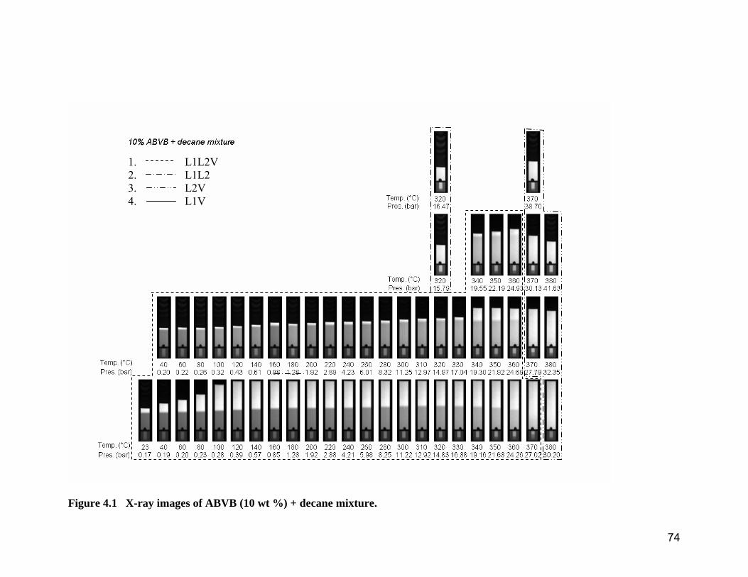
74
Figure 4.1 X-ray images of ABVB (10 wt %) + decane mixture.
1. L1L2V 2. L1L2 3. L2V 4. L1V
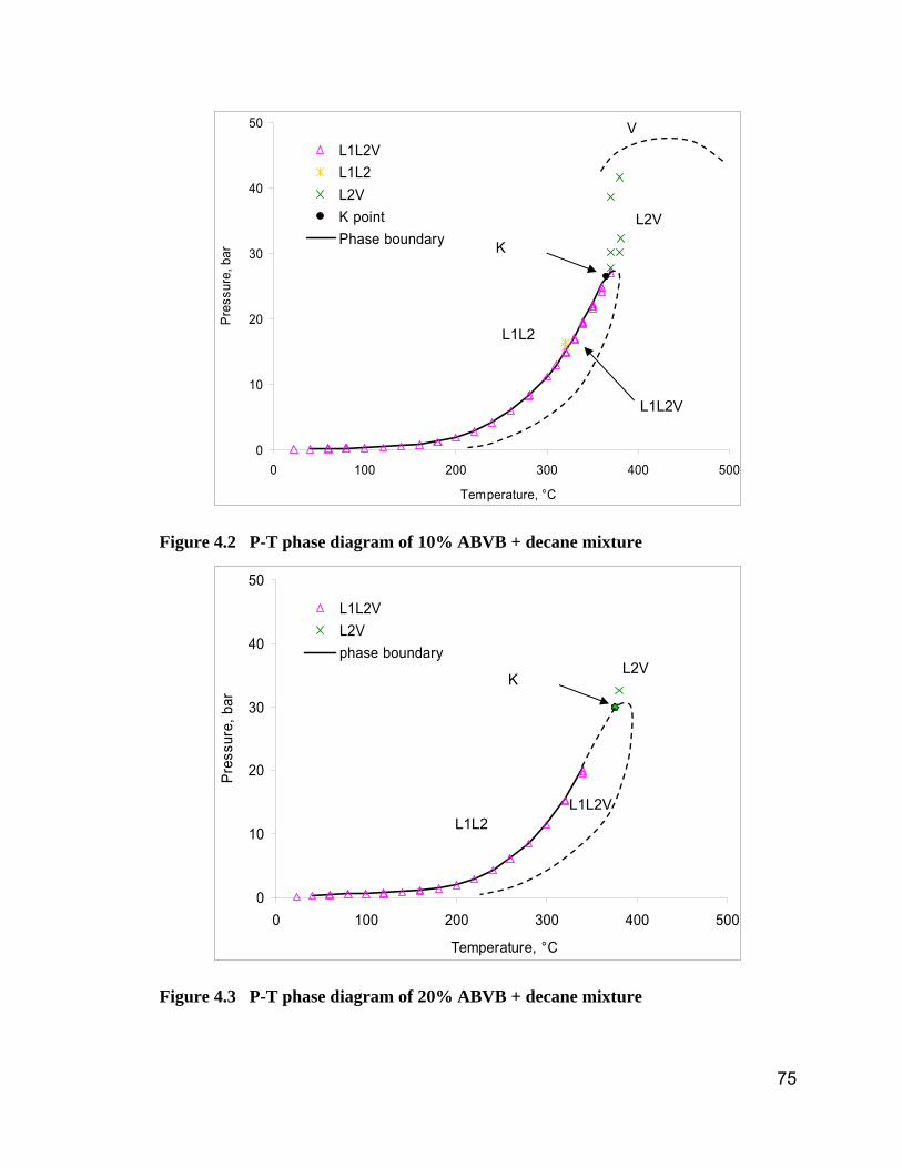
75
0
10
20
30
40
50
0 100 200 300 400 500
Temperature, °C
Pre
ssur
e, b
ar
L1L2VL1L2L2VK pointPhase boundary
Figure 4.2 P-T phase diagram of 10% ABVB + decane mixture
0
10
20
30
40
50
0 100 200 300 400 500
Temperature, °C
Pres
sure
, bar
L1L2VL2Vphase boundary
Figure 4.3 P-T phase diagram of 20% ABVB + decane mixture
L1L2V
L2V
L1L2
V
L1L2V
L2V
L1L2
K
K
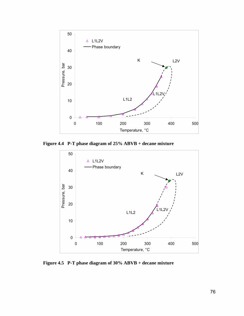
76
0
10
20
30
40
50
0 100 200 300 400 500Temperature, °C
Pres
sure
, bar
L1L2VPhase boundary
Figure 4.4 P-T phase diagram of 25% ABVB + decane mixture
0
10
20
30
40
50
0 100 200 300 400 500Temperature, °C
Pres
sure
, bar
L1L2VPhase boundary
Figure 4.5 P-T phase diagram of 30% ABVB + decane mixture
L1L2V
L2V
L1L2
K
L1L2V
L2V
L1L2
K
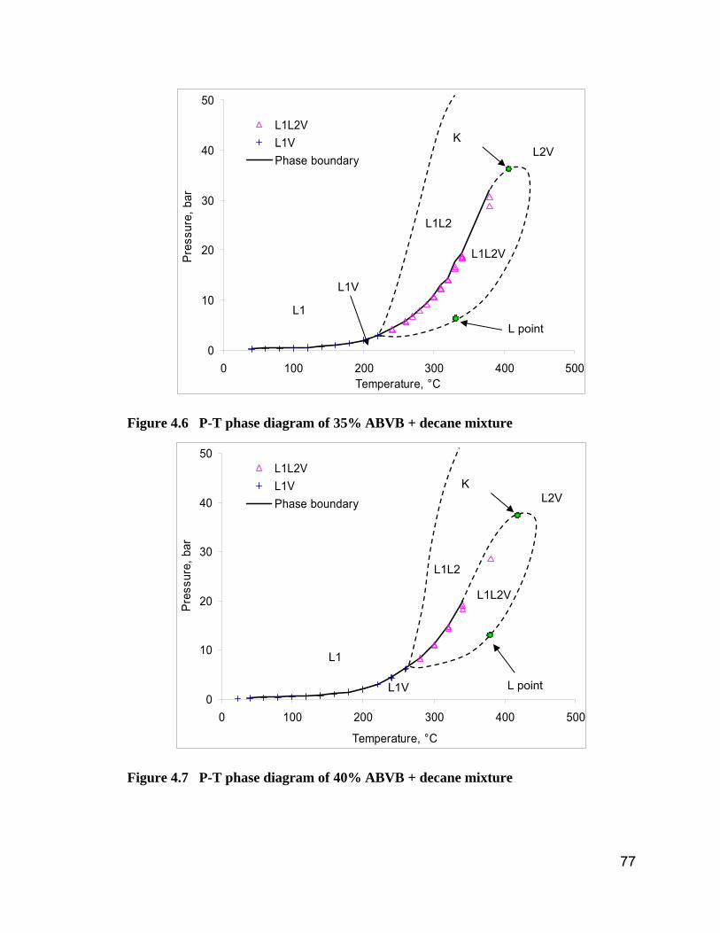
77
0
10
20
30
40
50
0 100 200 300 400 500Temperature, °C
Pres
sure
, bar
L1L2VL1VPhase boundary
Figure 4.6 P-T phase diagram of 35% ABVB + decane mixture
0
10
20
30
40
50
0 100 200 300 400 500
Temperature, °C
Pres
sure
, bar
L1L2VL1VPhase boundary
Figure 4.7 P-T phase diagram of 40% ABVB + decane mixture
L1L2V
L2V
L1L2
K
L1
L1V
L point
L1L2V
L2V
L1L2
K
L1
L1V L point
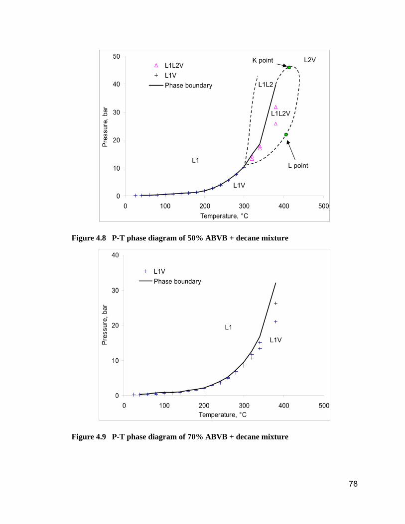
78
0
10
20
30
40
50
0 100 200 300 400 500Temperature, °C
Pres
sure
, bar
L1L2VL1VPhase boundary
Figure 4.8 P-T phase diagram of 50% ABVB + decane mixture
0
10
20
30
40
0 100 200 300 400 500Temperature, °C
Pres
sure
, bar
L1VPhase boundary
Figure 4.9 P-T phase diagram of 70% ABVB + decane mixture
L1L2V
L2V
L1L2
K point
L1
L1V
L point
L1
L1V
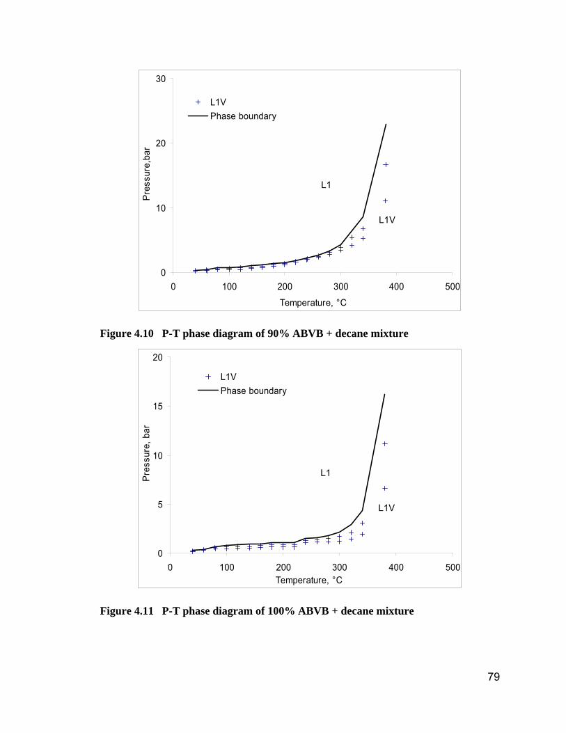
79
0
10
20
30
0 100 200 300 400 500
Temperature, °C
Pres
sure
,bar
L1VPhase boundary
Figure 4.10 P-T phase diagram of 90% ABVB + decane mixture
0
5
10
15
20
0 100 200 300 400 500Temperature, °C
Pres
sure
, bar
L1VPhase boundary
Figure 4.11 P-T phase diagram of 100% ABVB + decane mixture
L1
L1V
L1
L1V
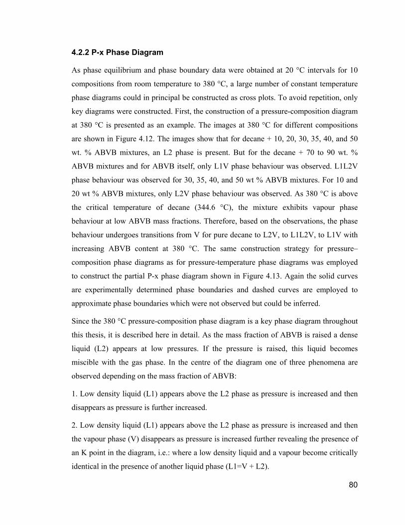
80
4.2.2 P-x Phase Diagram
As phase equilibrium and phase boundary data were obtained at 20 °C intervals for 10
compositions from room temperature to 380 °C, a large number of constant temperature
phase diagrams could in principal be constructed as cross plots. To avoid repetition, only
key diagrams were constructed. First, the construction of a pressure-composition diagram
at 380 °C is presented as an example. The images at 380 °C for different compositions
are shown in Figure 4.12. The images show that for decane + 10, 20, 30, 35, 40, and 50
wt. % ABVB mixtures, an L2 phase is present. But for the decane + 70 to 90 wt. %
ABVB mixtures and for ABVB itself, only L1V phase behaviour was observed. L1L2V
phase behaviour was observed for 30, 35, 40, and 50 wt % ABVB mixtures. For 10 and
20 wt % ABVB mixtures, only L2V phase behaviour was observed. As 380 °C is above
the critical temperature of decane (344.6 °C), the mixture exhibits vapour phase
behaviour at low ABVB mass fractions. Therefore, based on the observations, the phase
behaviour undergoes transitions from V for pure decane to L2V, to L1L2V, to L1V with
increasing ABVB content at 380 °C. The same construction strategy for pressure–
composition phase diagrams as for pressure-temperature phase diagrams was employed
to construct the partial P-x phase diagram shown in Figure 4.13. Again the solid curves
are experimentally determined phase boundaries and dashed curves are employed to
approximate phase boundaries which were not observed but could be inferred.
Since the 380 °C pressure-composition phase diagram is a key phase diagram throughout
this thesis, it is described here in detail. As the mass fraction of ABVB is raised a dense
liquid (L2) appears at low pressures. If the pressure is raised, this liquid becomes
miscible with the gas phase. In the centre of the diagram one of three phenomena are
observed depending on the mass fraction of ABVB:
1. Low density liquid (L1) appears above the L2 phase as pressure is increased and then
disappears as pressure is further increased.
2. Low density liquid (L1) appears above the L2 phase as pressure is increased and then
the vapour phase (V) disappears as pressure is increased further revealing the presence of
an K point in the diagram, i.e.: where a low density liquid and a vapour become critically
identical in the presence of another liquid phase (L1=V + L2).
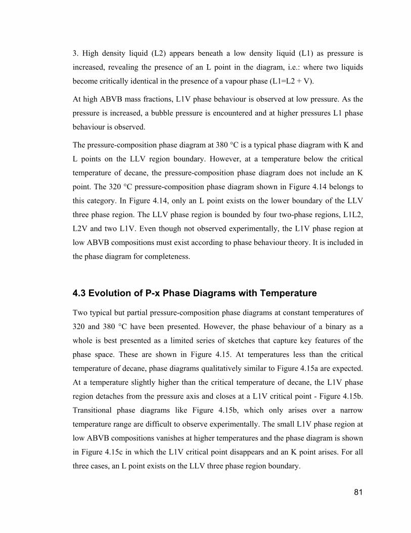
81
3. High density liquid (L2) appears beneath a low density liquid (L1) as pressure is
increased, revealing the presence of an L point in the diagram, i.e.: where two liquids
become critically identical in the presence of a vapour phase (L1=L2 + V).
At high ABVB mass fractions, L1V phase behaviour is observed at low pressure. As the
pressure is increased, a bubble pressure is encountered and at higher pressures L1 phase
behaviour is observed.
The pressure-composition phase diagram at 380 °C is a typical phase diagram with K and
L points on the LLV region boundary. However, at a temperature below the critical
temperature of decane, the pressure-composition phase diagram does not include an K
point. The 320 °C pressure-composition phase diagram shown in Figure 4.14 belongs to
this category. In Figure 4.14, only an L point exists on the lower boundary of the LLV
three phase region. The LLV phase region is bounded by four two-phase regions, L1L2,
L2V and two L1V. Even though not observed experimentally, the L1V phase region at
low ABVB compositions must exist according to phase behaviour theory. It is included in
the phase diagram for completeness.
4.3 Evolution of P-x Phase Diagrams with Temperature
Two typical but partial pressure-composition phase diagrams at constant temperatures of
320 and 380 °C have been presented. However, the phase behaviour of a binary as a
whole is best presented as a limited series of sketches that capture key features of the
phase space. These are shown in Figure 4.15. At temperatures less than the critical
temperature of decane, phase diagrams qualitatively similar to Figure 4.15a are expected.
At a temperature slightly higher than the critical temperature of decane, the L1V phase
region detaches from the pressure axis and closes at a L1V critical point - Figure 4.15b.
Transitional phase diagrams like Figure 4.15b, which only arises over a narrow
temperature range are difficult to observe experimentally. The small L1V phase region at
low ABVB compositions vanishes at higher temperatures and the phase diagram is shown
in Figure 4.15c in which the L1V critical point disappears and an K point arises. For all
three cases, an L point exists on the LLV three phase region boundary.
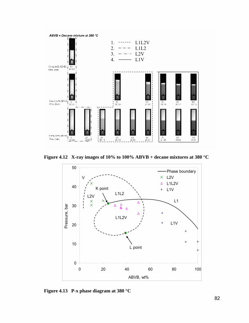
82
Figure 4.12 X-ray images of 10% to 100% ABVB + decane mixtures at 380 °C
0
10
20
30
40
50
0 20 40 60 80 100
ABVB, wt%
Pres
sure
, bar
Phase boundaryL2VL1L2VL1V
L1L2VL1V
L2V L1L2
L1
V
K point
L point
Figure 4.13 P-x phase diagram at 380 °C
1. L1L2V 2. L1L2 3. L2V 4. L1V
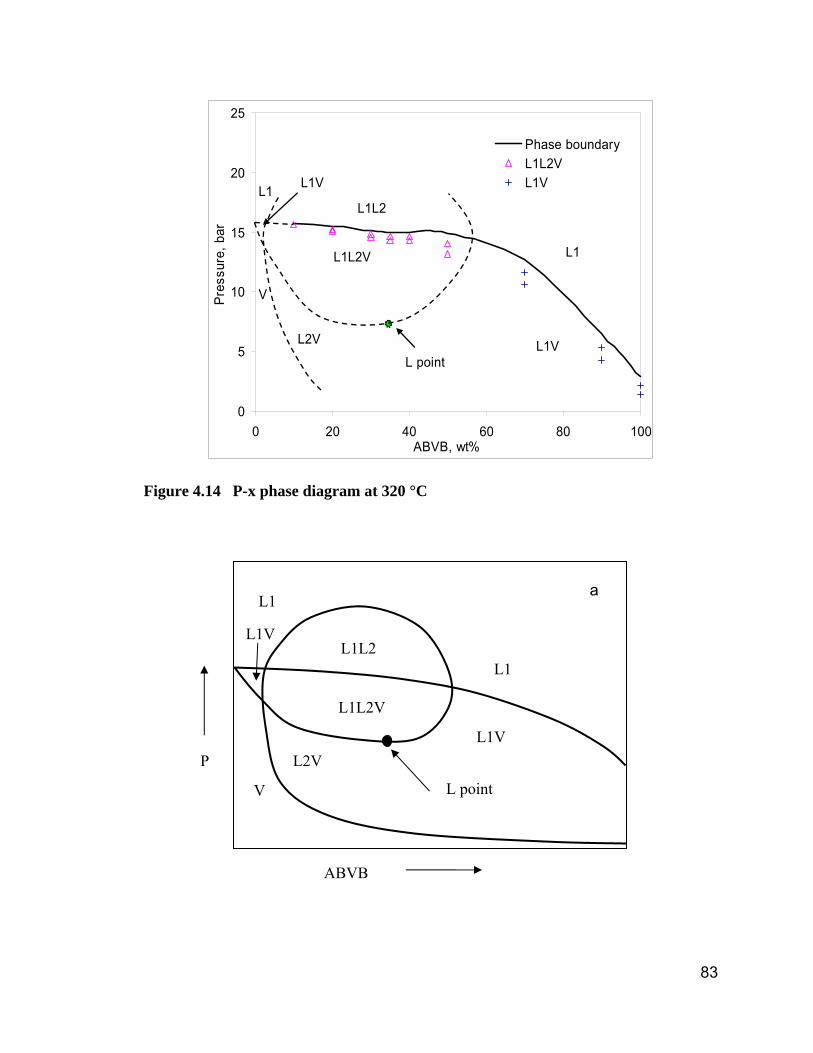
83
0
5
10
15
20
25
0 20 40 60 80 100ABVB, wt%
Pres
sure
, bar
Phase boundaryL1L2VL1V
L1L2V
L1V
L1L2
V
L1
L1
L1VL2V
L point
Figure 4.14 P-x phase diagram at 320 °C
ABVB
P L1V
L1
L1L2V
L1L2
L2V
L1
V
L1V
L point
a
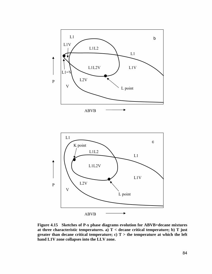
84
Figure 4.15 Sketches of P-x phase diagrams evolution for ABVB+decane mixtures at three characteristic temperatures. a) T < decane critical temperature; b) T just greater than decane critical temperature; c) T > the temperature at which the left hand L1V zone collapses into the LLV zone.
ABVB
P
L1V
L1
L1L2V
L1L2
L2V
L1
V L point
K point c
ABVB
P
L1V
L1
L1L2V
L1L2
L2V
L1
V
L1V
L point
L1=V
b
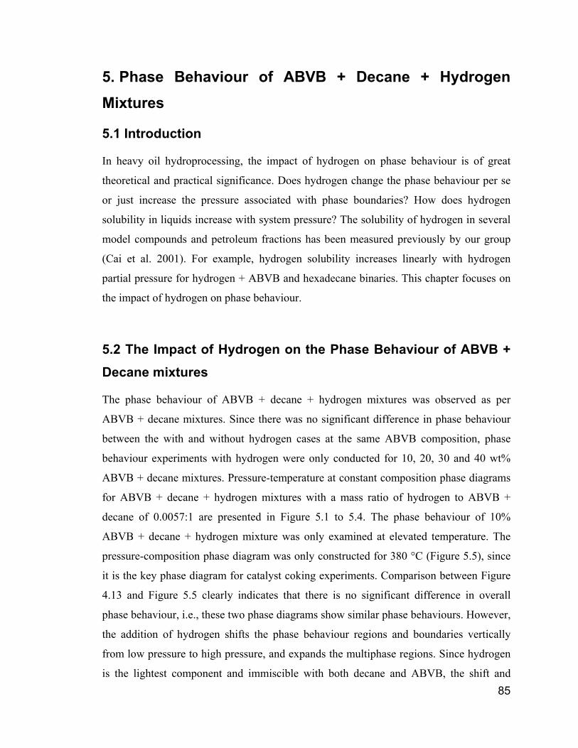
85
5. Phase Behaviour of ABVB + Decane + Hydrogen Mixtures
5.1 Introduction
In heavy oil hydroprocessing, the impact of hydrogen on phase behaviour is of great
theoretical and practical significance. Does hydrogen change the phase behaviour per se
or just increase the pressure associated with phase boundaries? How does hydrogen
solubility in liquids increase with system pressure? The solubility of hydrogen in several
model compounds and petroleum fractions has been measured previously by our group
(Cai et al. 2001). For example, hydrogen solubility increases linearly with hydrogen
partial pressure for hydrogen + ABVB and hexadecane binaries. This chapter focuses on
the impact of hydrogen on phase behaviour.
5.2 The Impact of Hydrogen on the Phase Behaviour of ABVB + Decane mixtures
The phase behaviour of ABVB + decane + hydrogen mixtures was observed as per
ABVB + decane mixtures. Since there was no significant difference in phase behaviour
between the with and without hydrogen cases at the same ABVB composition, phase
behaviour experiments with hydrogen were only conducted for 10, 20, 30 and 40 wt%
ABVB + decane mixtures. Pressure-temperature at constant composition phase diagrams
for ABVB + decane + hydrogen mixtures with a mass ratio of hydrogen to ABVB +
decane of 0.0057:1 are presented in Figure 5.1 to 5.4. The phase behaviour of 10%
ABVB + decane + hydrogen mixture was only examined at elevated temperature. The
pressure-composition phase diagram was only constructed for 380 °C (Figure 5.5), since
it is the key phase diagram for catalyst coking experiments. Comparison between Figure
4.13 and Figure 5.5 clearly indicates that there is no significant difference in overall
phase behaviour, i.e., these two phase diagrams show similar phase behaviours. However,
the addition of hydrogen shifts the phase behaviour regions and boundaries vertically
from low pressure to high pressure, and expands the multiphase regions. Since hydrogen
is the lightest component and immiscible with both decane and ABVB, the shift and
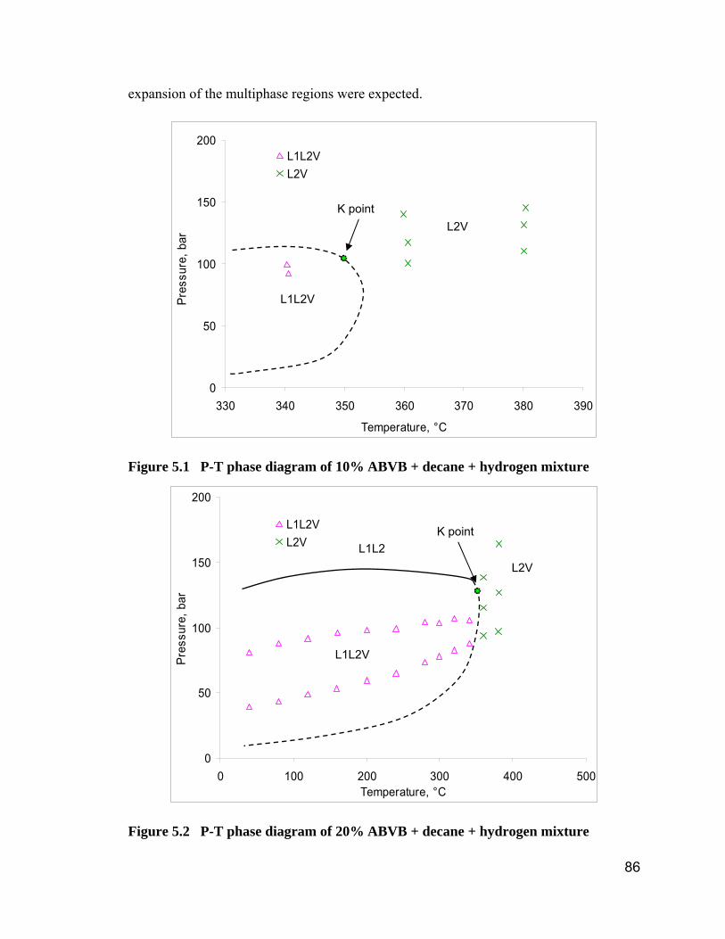
86
expansion of the multiphase regions were expected.
0
50
100
150
200
330 340 350 360 370 380 390
Temperature, °C
Pres
sure
, bar
L1L2VL2V
Figure 5.1 P-T phase diagram of 10% ABVB + decane + hydrogen mixture
0
50
100
150
200
0 100 200 300 400 500Temperature, °C
Pres
sure
, bar
L1L2VL2V
Figure 5.2 P-T phase diagram of 20% ABVB + decane + hydrogen mixture
L1L2V
L2V
L1L2V
L2V L1L2
K point
K point
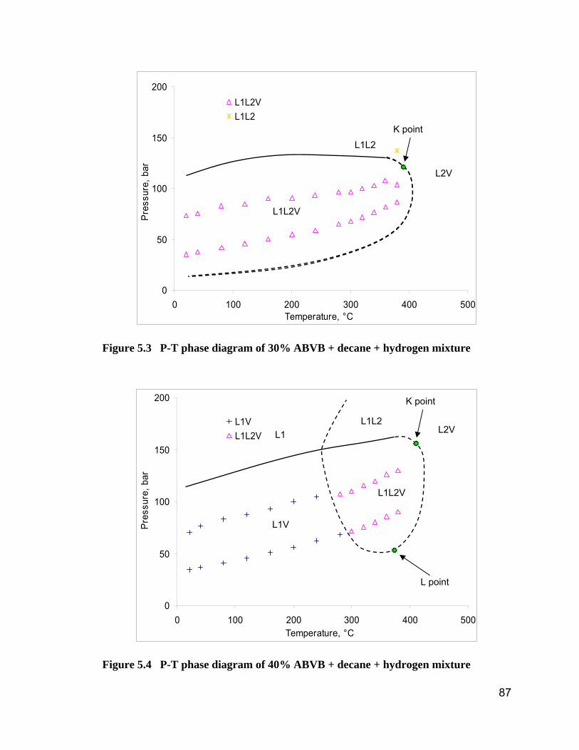
87
0
50
100
150
200
0 100 200 300 400 500Temperature, °C
Pres
sure
, bar
L1L2VL1L2
Figure 5.3 P-T phase diagram of 30% ABVB + decane + hydrogen mixture
0
50
100
150
200
0 100 200 300 400 500Temperature, °C
Pres
sure
, bar
L1VL1L2V
Figure 5.4 P-T phase diagram of 40% ABVB + decane + hydrogen mixture
L1L2V
L2V
L1L2V
L2V
L1V
L1L1L2
K point
L point
L1L2K point
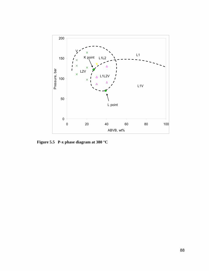
88
0
50
100
150
200
0 20 40 60 80 100
ABVB, wt%
Pres
sure
, bar
L1L2V
L1V
L2V
L1L2L1
V
K point
L point
Figure 5.5 P-x phase diagram at 380 °C
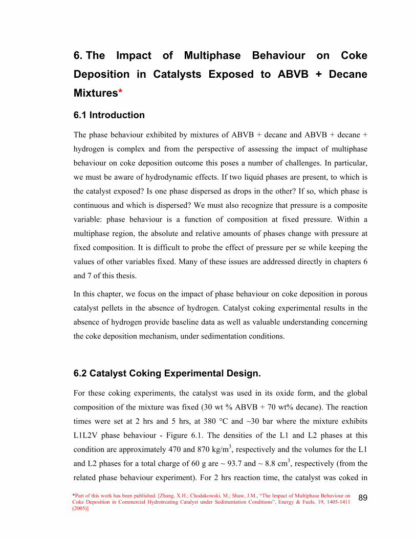
89
6. The Impact of Multiphase Behaviour on Coke Deposition in Catalysts Exposed to ABVB + Decane Mixtures*
6.1 Introduction
The phase behaviour exhibited by mixtures of ABVB + decane and ABVB + decane +
hydrogen is complex and from the perspective of assessing the impact of multiphase
behaviour on coke deposition outcome this poses a number of challenges. In particular,
we must be aware of hydrodynamic effects. If two liquid phases are present, to which is
the catalyst exposed? Is one phase dispersed as drops in the other? If so, which phase is
continuous and which is dispersed? We must also recognize that pressure is a composite
variable: phase behaviour is a function of composition at fixed pressure. Within a
multiphase region, the absolute and relative amounts of phases change with pressure at
fixed composition. It is difficult to probe the effect of pressure per se while keeping the
values of other variables fixed. Many of these issues are addressed directly in chapters 6
and 7 of this thesis.
In this chapter, we focus on the impact of phase behaviour on coke deposition in porous
catalyst pellets in the absence of hydrogen. Catalyst coking experimental results in the
absence of hydrogen provide baseline data as well as valuable understanding concerning
the coke deposition mechanism, under sedimentation conditions.
6.2 Catalyst Coking Experimental Design.
For these coking experiments, the catalyst was used in its oxide form, and the global
composition of the mixture was fixed (30 wt % ABVB + 70 wt% decane). The reaction
times were set at 2 hrs and 5 hrs, at 380 °C and ~30 bar where the mixture exhibits
L1L2V phase behaviour - Figure 6.1. The densities of the L1 and L2 phases at this
condition are approximately 470 and 870 kg/m3, respectively and the volumes for the L1
and L2 phases for a total charge of 60 g are ~ 93.7 and ~ 8.8 cm3, respectively (from the
related phase behaviour experiment). For 2 hrs reaction time, the catalyst was coked in
*Part of this work has been published. [Zhang, X.H.; Chodakowski, M.; Shaw, J.M., “The Impact of Multiphase Behaviour on Coke Deposition in Commercial Hydrotreating Catalyst under Sedimentation Conditions”, Energy & Fuels, 19, 1405-1411 (2005)]
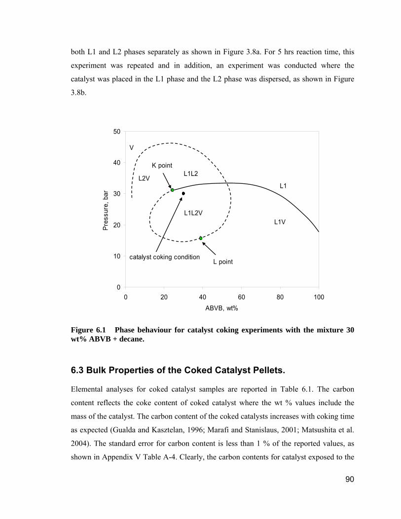
90
both L1 and L2 phases separately as shown in Figure 3.8a. For 5 hrs reaction time, this
experiment was repeated and in addition, an experiment was conducted where the
catalyst was placed in the L1 phase and the L2 phase was dispersed, as shown in Figure
3.8b.
0
10
20
30
40
50
0 20 40 60 80 100ABVB, wt%
Pres
sure
, bar
L1L2VL1V
L2VL1L2
L1
V
K point
L pointcatalyst coking condition
Figure 6.1 Phase behaviour for catalyst coking experiments with the mixture 30 wt% ABVB + decane.
6.3 Bulk Properties of the Coked Catalyst Pellets.
Elemental analyses for coked catalyst samples are reported in Table 6.1. The carbon
content reflects the coke content of coked catalyst where the wt % values include the
mass of the catalyst. The carbon content of the coked catalysts increases with coking time
as expected (Gualda and Kasztelan, 1996; Marafi and Stanislaus, 2001; Matsushita et al.
2004). The standard error for carbon content is less than 1 % of the reported values, as
shown in Appendix V Table A-4. Clearly, the carbon contents for catalyst exposed to the
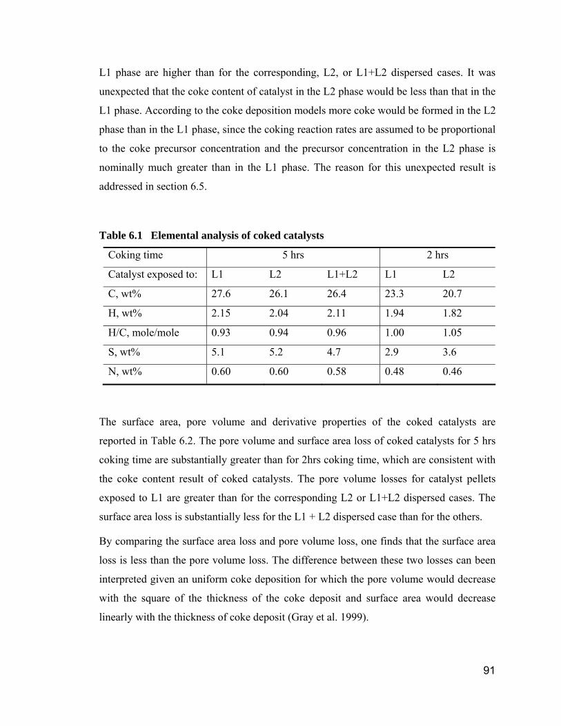
91
L1 phase are higher than for the corresponding, L2, or L1+L2 dispersed cases. It was
unexpected that the coke content of catalyst in the L2 phase would be less than that in the
L1 phase. According to the coke deposition models more coke would be formed in the L2
phase than in the L1 phase, since the coking reaction rates are assumed to be proportional
to the coke precursor concentration and the precursor concentration in the L2 phase is
nominally much greater than in the L1 phase. The reason for this unexpected result is
addressed in section 6.5.
Table 6.1 Elemental analysis of coked catalysts
Coking time 5 hrs 2 hrs
Catalyst exposed to: L1 L2 L1+L2 L1 L2
C, wt% 27.6 26.1 26.4 23.3 20.7
H, wt% 2.15 2.04 2.11 1.94 1.82
H/C, mole/mole 0.93 0.94 0.96 1.00 1.05
S, wt% 5.1 5.2 4.7 2.9 3.6
N, wt% 0.60 0.60 0.58 0.48 0.46
The surface area, pore volume and derivative properties of the coked catalysts are
reported in Table 6.2. The pore volume and surface area loss of coked catalysts for 5 hrs
coking time are substantially greater than for 2hrs coking time, which are consistent with
the coke content result of coked catalysts. The pore volume losses for catalyst pellets
exposed to L1 are greater than for the corresponding L2 or L1+L2 dispersed cases. The
surface area loss is substantially less for the L1 + L2 dispersed case than for the others.
By comparing the surface area loss and pore volume loss, one finds that the surface area
loss is less than the pore volume loss. The difference between these two losses can been
interpreted given an uniform coke deposition for which the pore volume would decrease
with the square of the thickness of the coke deposit and surface area would decrease
linearly with the thickness of coke deposit (Gray et al. 1999).
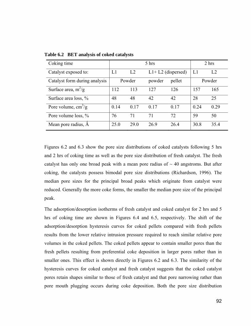
92
Table 6.2 BET analysis of coked catalysts
Coking time 5 hrs 2 hrs
Catalyst exposed to: L1 L2 L1+ L2 (dispersed) L1 L2
Catalyst form during analysis Powder powder pellet Powder
Surface area, m2/g 112 113 127 126 157 165
Surface area loss, % 48 48 42 42 28 25
Pore volume, cm3/g 0.14 0.17 0.17 0.17 0.24 0.29
Pore volume loss, % 76 71 71 72 59 50
Mean pore radius, Ǻ 25.0 29.0 26.9 26.4 30.8 35.4
Figures 6.2 and 6.3 show the pore size distributions of coked catalysts following 5 hrs
and 2 hrs of coking time as well as the pore size distribution of fresh catalyst. The fresh
catalyst has only one broad peak with a mean pore radius of ~ 40 angstroms. But after
coking, the catalysts possess bimodal pore size distributions (Richardson, 1996). The
median pore sizes for the principal broad peaks which originate from catalyst were
reduced. Generally the more coke forms, the smaller the median pore size of the principal
peak.
The adsorption/desorption isotherms of fresh catalyst and coked catalyst for 2 hrs and 5
hrs of coking time are shown in Figures 6.4 and 6.5, respectively. The shift of the
adsorption/desorption hysteresis curves for coked pellets compared with fresh pellets
results from the lower relative intrusion pressure required to reach similar relative pore
volumes in the coked pellets. The coked pellets appear to contain smaller pores than the
fresh pellets resulting from preferential coke deposition in larger pores rather than in
smaller ones. This effect is shown directly in Figures 6.2 and 6.3. The similarity of the
hysteresis curves for coked catalyst and fresh catalyst suggests that the coked catalyst
pores retain shapes similar to those of fresh catalyst and that pore narrowing rather than
pore mouth plugging occurs during coke deposition. Both the pore size distribution
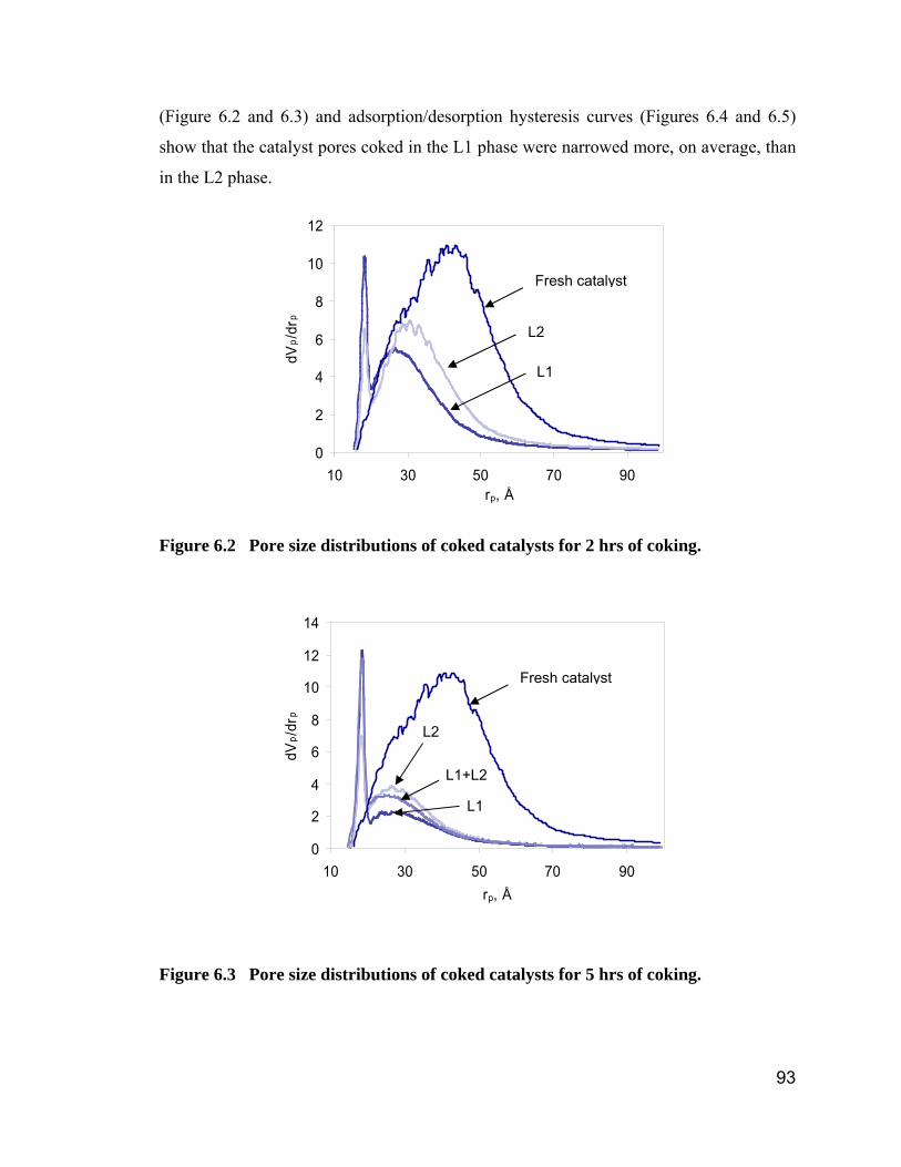
93
(Figure 6.2 and 6.3) and adsorption/desorption hysteresis curves (Figures 6.4 and 6.5)
show that the catalyst pores coked in the L1 phase were narrowed more, on average, than
in the L2 phase.
0
2
4
6
8
10
12
10 30 50 70 90rp, Å
dVp /
drp
Figure 6.2 Pore size distributions of coked catalysts for 2 hrs of coking.
0
2
4
6
8
10
12
14
10 30 50 70 90rp, Å
dVp /
drp
Figure 6.3 Pore size distributions of coked catalysts for 5 hrs of coking.
Fresh catalyst
L2
L1
Fresh catalyst
L2
L1
L1+L2
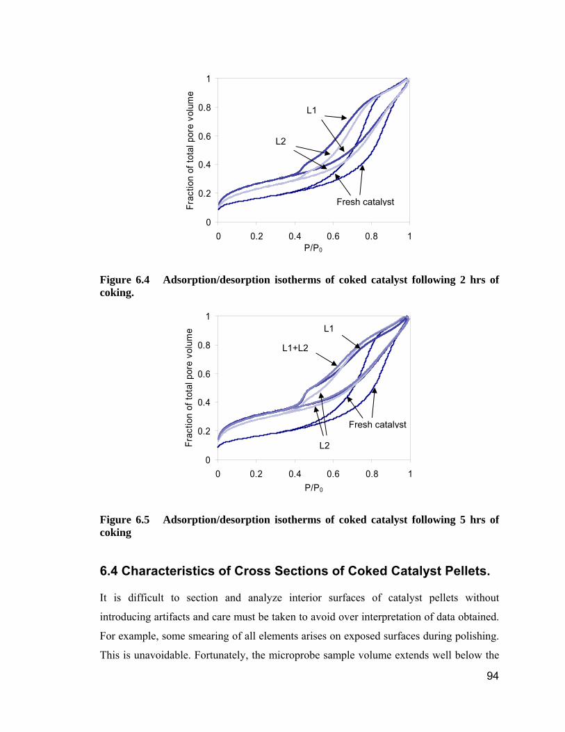
94
0
0.2
0.4
0.6
0.8
1
0 0.2 0.4 0.6 0.8 1P/P0
Frac
tion
of to
tal p
ore
volu
me
Figure 6.4 Adsorption/desorption isotherms of coked catalyst following 2 hrs of coking.
0
0.2
0.4
0.6
0.8
1
0 0.2 0.4 0.6 0.8 1P/P0
Frac
tion
of to
tal p
ore
volu
me
Figure 6.5 Adsorption/desorption isotherms of coked catalyst following 5 hrs of coking
6.4 Characteristics of Cross Sections of Coked Catalyst Pellets.
It is difficult to section and analyze interior surfaces of catalyst pellets without
introducing artifacts and care must be taken to avoid over interpretation of data obtained.
For example, some smearing of all elements arises on exposed surfaces during polishing.
This is unavoidable. Fortunately, the microprobe sample volume extends well below the
Fresh catalyst
L2
L1
Fresh catalyst
L2
L1
L1+L2
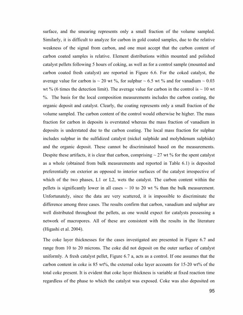
95
surface, and the smearing represents only a small fraction of the volume sampled.
Similarly, it is difficult to analyze for carbon in gold coated samples, due to the relative
weakness of the signal from carbon, and one must accept that the carbon content of
carbon coated samples is relative. Element distributions within mounted and polished
catalyst pellets following 5 hours of coking, as well as for a control sample (mounted and
carbon coated fresh catalyst) are reported in Figure 6.6. For the coked catalyst, the
average value for carbon is ~ 20 wt %, for sulphur ~ 6.5 wt % and for vanadium ~ 0.03
wt % (6 times the detection limit). The average value for carbon in the control is ~ 10 wt
%. The basis for the local composition measurements includes the carbon coating, the
organic deposit and catalyst. Clearly, the coating represents only a small fraction of the
volume sampled. The carbon content of the control would otherwise be higher. The mass
fraction for carbon in deposits is overstated whereas the mass fraction of vanadium in
deposits is understated due to the carbon coating. The local mass fraction for sulphur
includes sulphur in the sulfidized catalyst (nickel sulphide and molybdenum sulphide)
and the organic deposit. These cannot be discriminated based on the measurements.
Despite these artifacts, it is clear that carbon, comprising ~ 27 wt % for the spent catalyst
as a whole (obtained from bulk measurements and reported in Table 6.1) is deposited
preferentially on exterior as opposed to interior surfaces of the catalyst irrespective of
which of the two phases, L1 or L2, wets the catalyst. The carbon content within the
pellets is significantly lower in all cases ~ 10 to 20 wt % than the bulk measurement.
Unfortunately, since the data are very scattered, it is impossible to discriminate the
difference among three cases. The results confirm that carbon, vanadium and sulphur are
well distributed throughout the pellets, as one would expect for catalysts possessing a
network of macropores. All of these are consistent with the results in the literature
(Higashi et al. 2004).
The coke layer thicknesses for the cases investigated are presented in Figure 6.7 and
range from 10 to 20 microns. The coke did not deposit on the outer surface of catalyst
uniformly. A fresh catalyst pellet, Figure 6.7 a, acts as a control. If one assumes that the
carbon content in coke is 85 wt%, the external coke layer accounts for 15-20 wt% of the
total coke present. It is evident that coke layer thickness is variable at fixed reaction time
regardless of the phase to which the catalyst was exposed. Coke was also deposited on
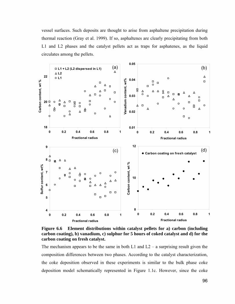
96
vessel surfaces. Such deposits are thought to arise from asphaltene precipitation during
thermal reaction (Gray et al. 1999). If so, asphaltenes are clearly precipitating from both
L1 and L2 phases and the catalyst pellets act as traps for asphatenes, as the liquid
circulates among the pellets.
Figure 6.6 Element distributions within catalyst pellets for a) carbon (including carbon coating), b) vanadium, c) sulphur for 5 hours of coked catalyst and d) for the carbon coating on fresh catalyst. The mechanism appears to be the same in both L1 and L2 – a surprising result given the
composition differences between two phases. According to the catalyst characterization,
the coke deposition observed in these experiments is similar to the bulk phase coke
deposition model schematically represented in Figure 1.1c. However, since the coke
0.01
0.02
0.03
0.04
0.05
0 0.2 0.4 0.6 0.8 1
Fractional radius
Vana
dium
con
tent
, wt%
18
20
22
0 0.2 0.4 0.6 0.8 1
Fractional radius
Car
bon
cont
ent,
wt %
L1 + L2 (L2 dispersed in L1)L2L1
4
5
6
7
8
9
0 0.2 0.4 0.6 0.8 1
Fractional radius
Sulfu
r con
tent
, wt%
8
10
12
0 0.2 0.4 0.6 0.8 1
Fractional radius
Car
bon
cont
ent,
wt %
Carbon coating on fresh catalyst
(a) (b)
(c) (d)
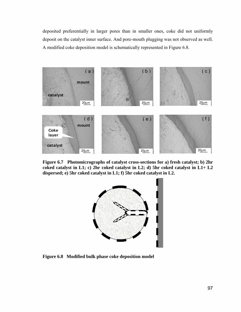
97
deposited preferentially in larger pores than in smaller ones, coke did not uniformly
deposit on the catalyst inner surface. And pore-mouth plugging was not observed as well.
A modified coke deposition model is schematically represented in Figure 6.8.
Figure 6.7 Photomicrographs of catalyst cross-sections for a) fresh catalyst; b) 2hr coked catalyst in L1; c) 2hr coked catalyst in L2; d) 5hr coked catalyst in L1+ L2 dispersed; e) 5hr coked catalyst in L1; f) 5hr coked catalyst in L2.
Figure 6.8 Modified bulk phase coke deposition model
catalyst
mount Coke layer
catalyst
mount
( a ) ( b )
( d ) ( e )
20μm 20μm 20μm
20μm 20μm 20μm
( c )
( f )
98
6.5 Possible Explanations for Greater Deposition in Catalysts Exposed to L1 vs L2
The carbon contents, surface area and pore volume losses for catalyst pellets exposed to
L1 are greater than for the corresponding L2 case. As the mass of the catalyst is small
compared to the mass of the bulk phases and the mass of coke precursors present in each
phase, and the residence times are relatively long, one may examine transport processes
for an explanation of the above results. The viscosity of the L1 phase (a solvent-rich
phase) is less than the viscosity of the L2 phase (an asphaltene-rich phase). One is
tempted to assert that therefore L1 circulates more readily within the macropores of the
pellets facilitating asphaltene transport and hence coke deposition. High-temperature
viscosity data for bitumen combined with a variety of alkane solvents does not support
this assertion as the viscosities of both phases at 380 °C are low – less than 2 mPa-s
(Seyer and Gyte, 1989). An alternative explanation must be sought for these results.
Asphaltene aggregates size may play an important role at the beginning of coking. A
fraction of asphaltene aggregates present in heavy oils are small enough to be observed
by SAXS measurements. Figure 6.9 shows scatterer size distribution data for ABVB and
ABVB (5 wt %) + dodecane. The method is limited to scatterers with leading dimensions
in the 10 Å to 1000 Å size range. While the conditions are not identical to the ones
employed in the coking experiments, it is clear that a greater fraction of smaller scatterers
is present in ABVB diluted in dodecane over a broad range of temperatures than in the
parent oil under similar conditions. Further, the leading dimensions of these small
scatterers fall well within the size range of catalyst pores. Thus, the average scatterers
present in L1 (the dilute ABVB phase) may penetrate the catalyst more readily than the
average ones present in L2 (the more concentrated ABVB phase). This difference readily
accounts for the greater pore area and pore volume loss, and coke content within pellets
for the L1 vs. L2 cases. After a coke layer is formed on the catalyst outer surface, the
asphaltene aggregates do not further affect coking in the pellet interior. It is also well
known that the deposit at the early stage of the catalyst fouling process is deposited
reversibly and desorbs under favourable operating conditions. Thus the solubility of
initial deposits in the surrounding liquid phase may also play a role. Since the L2 phase
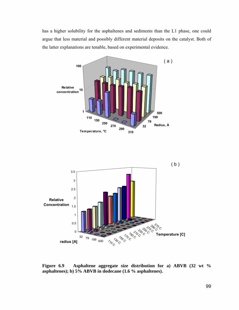
99
has a higher solubility for the asphaltenes and sediments than the L1 phase, one could
argue that less material and possibly different material deposits on the catalyst. Both of
the latter explanations are tenable, based on experimental evidence.
110150
250270
290310
3279
1995001
10
100
Relative concentration
Temperature, °C
Radius, Å
Figure 6.9 Asphaltene aggregate size distribution for a) ABVB (32 wt % asphaltenes); b) 5% ABVB in dodecane (1.6 % asphaltenes).
( a )
( b )
32 79 199 500 110 C
130 C
150 C
170 C
190 C
210 C
230 C
250 C
270 C290 C
310 C0
0.5
1
1.5
2
2.5
3
3.5
Relative Concentration
radius [A]
Temperature [C]
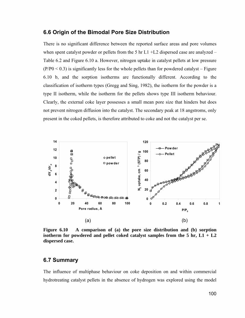
100
0
20
40
60
80
100
120
0 0.2 0.4 0.6 0.8 1
P/P0
N 2 u
ptak
e, c
m3 (S
TP) /
g
Pow derPelle t
6.6 Origin of the Bimodal Pore Size Distribution
There is no significant difference between the reported surface areas and pore volumes
when spent catalyst powder or pellets from the 5 hr L1 +L2 dispersed case are analyzed –
Table 6.2 and Figure 6.10 a. However, nitrogen uptake in catalyst pellets at low pressure
(P/P0 < 0.3) is significantly less for the whole pellets than for powdered catalyst – Figure
6.10 b, and the sorption isotherms are functionally different. According to the
classification of isotherm types (Gregg and Sing, 1982), the isotherm for the powder is a
type II isotherm, while the isotherm for the pellets shows type III isotherm behaviour.
Clearly, the external coke layer possesses a small mean pore size that hinders but does
not prevent nitrogen diffusion into the catalyst. The secondary peak at 18 angstroms, only
present in the coked pellets, is therefore attributed to coke and not the catalyst per se.
0
2
4
6
8
10
12
14
0 20 40 60 80 100Pore radius, Å
dVp/d
r p
pe lle tpow der
Figure 6.10 A comparison of (a) the pore size distribution and (b) sorption isotherm for powdered and pellet coked catalyst samples from the 5 hr, L1 + L2 dispersed case.
6.7 Summary
The influence of multiphase behaviour on coke deposition on and within commercial
hydrotreating catalyst pellets in the absence of hydrogen was explored using the model
(a) (b)
101
mixture Athabasca vacuum bottoms (ABVB) + decane. Under these conditions, the
impact of phase behaviour on the amount of coke deposited on and within catalyst pellets
and the distribution of coke within catalyst pellets was found to be a secondary one
despite the differences in the physical properties of the solvent rich L1 phase and
asphaltene rich L2 phase. In all cases, the exterior surfaces of pellets were coated with a
thick nanoporous deposit layer. Observed differences in mean pore size, pore surface area
and pore volume of coked catalyst exposed to the L1 and L2 phases and to multiphase
environments are consistent with observed differences in the asphaltene aggregate size
distribution and asphaltene solubility in the two phases.
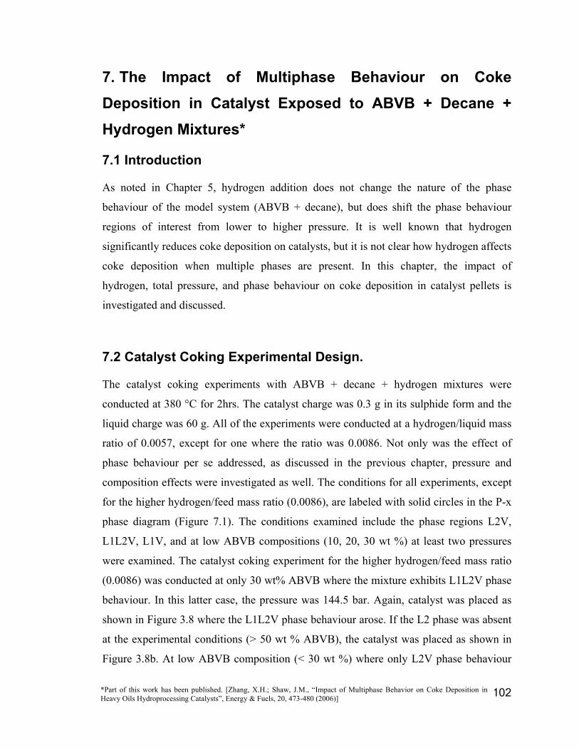
102
7. The Impact of Multiphase Behaviour on Coke Deposition in Catalyst Exposed to ABVB + Decane + Hydrogen Mixtures*
7.1 Introduction
As noted in Chapter 5, hydrogen addition does not change the nature of the phase
behaviour of the model system (ABVB + decane), but does shift the phase behaviour
regions of interest from lower to higher pressure. It is well known that hydrogen
significantly reduces coke deposition on catalysts, but it is not clear how hydrogen affects
coke deposition when multiple phases are present. In this chapter, the impact of
hydrogen, total pressure, and phase behaviour on coke deposition in catalyst pellets is
investigated and discussed.
7.2 Catalyst Coking Experimental Design.
The catalyst coking experiments with ABVB + decane + hydrogen mixtures were
conducted at 380 °C for 2hrs. The catalyst charge was 0.3 g in its sulphide form and the
liquid charge was 60 g. All of the experiments were conducted at a hydrogen/liquid mass
ratio of 0.0057, except for one where the ratio was 0.0086. Not only was the effect of
phase behaviour per se addressed, as discussed in the previous chapter, pressure and
composition effects were investigated as well. The conditions for all experiments, except
for the higher hydrogen/feed mass ratio (0.0086), are labeled with solid circles in the P-x
phase diagram (Figure 7.1). The conditions examined include the phase regions L2V,
L1L2V, L1V, and at low ABVB compositions (10, 20, 30 wt %) at least two pressures
were examined. The catalyst coking experiment for the higher hydrogen/feed mass ratio
(0.0086) was conducted at only 30 wt% ABVB where the mixture exhibits L1L2V phase
behaviour. In this latter case, the pressure was 144.5 bar. Again, catalyst was placed as
shown in Figure 3.8 where the L1L2V phase behaviour arose. If the L2 phase was absent
at the experimental conditions (> 50 wt % ABVB), the catalyst was placed as shown in
Figure 3.8b. At low ABVB composition (< 30 wt %) where only L2V phase behaviour
*Part of this work has been published. [Zhang, X.H.; Shaw, J.M., “Impact of Multiphase Behavior on Coke Deposition in Heavy Oils Hydroprocessing Catalysts”, Energy & Fuels, 20, 473-480 (2006)]
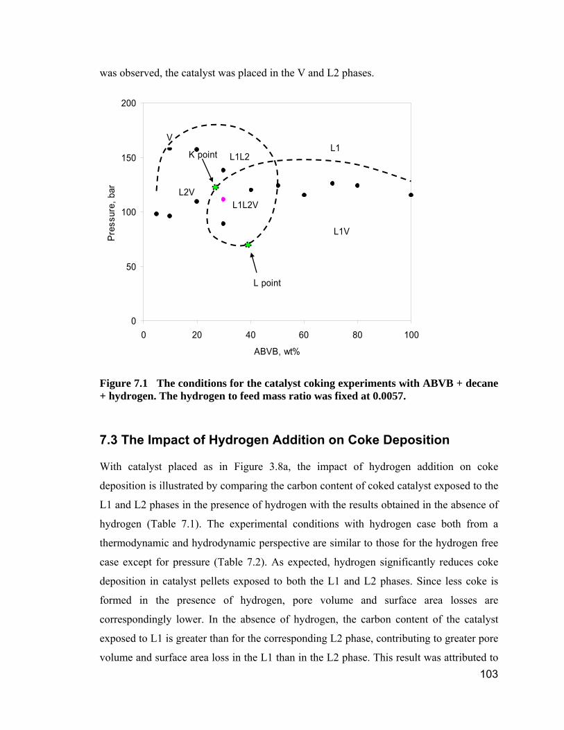
103
was observed, the catalyst was placed in the V and L2 phases.
0
50
100
150
200
0 20 40 60 80 100
ABVB, wt%
Pres
sure
, bar
L1L2V
L1V
L2V
L1L2L1
V
K point
L point
Figure 7.1 The conditions for the catalyst coking experiments with ABVB + decane + hydrogen. The hydrogen to feed mass ratio was fixed at 0.0057.
7.3 The Impact of Hydrogen Addition on Coke Deposition
With catalyst placed as in Figure 3.8a, the impact of hydrogen addition on coke
deposition is illustrated by comparing the carbon content of coked catalyst exposed to the
L1 and L2 phases in the presence of hydrogen with the results obtained in the absence of
hydrogen (Table 7.1). The experimental conditions with hydrogen case both from a
thermodynamic and hydrodynamic perspective are similar to those for the hydrogen free
case except for pressure (Table 7.2). As expected, hydrogen significantly reduces coke
deposition in catalyst pellets exposed to both the L1 and L2 phases. Since less coke is
formed in the presence of hydrogen, pore volume and surface area losses are
correspondingly lower. In the absence of hydrogen, the carbon content of the catalyst
exposed to L1 is greater than for the corresponding L2 phase, contributing to greater pore
volume and surface area loss in the L1 than in the L2 phase. This result was attributed to
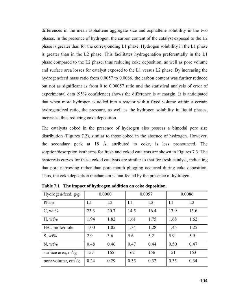
104
differences in the mean asphaltene aggregate size and asphaltene solubility in the two
phases. In the presence of hydrogen, the carbon content of the catalyst exposed to the L2
phase is greater than for the corresponding L1 phase. Hydrogen solubility in the L1 phase
is greater than in the L2 phase. This facilitates hydrogenation preferentially in the L1
phase compared to the L2 phase, thus reducing coke deposition, as well as pore volume
and surface area losses for catalyst exposed to the L1 versus L2 phase. By increasing the
hydrogen/feed mass ratio from 0.0057 to 0.0086, the carbon content was further reduced
but not as significant as from 0 to 0.00057 ratio and the statistical analysis of error of
experimental data (95% confidence) shows the difference is at margin. It is anticipated
that when more hydrogen is added into a reactor with a fixed volume within a certain
hydrogen/feed ratio, the pressure, as well as the hydrogen solubility in liquid phases,
increases, thus reducing coke deposition.
The catalysts coked in the presence of hydrogen also possess a bimodal pore size
distribution (Figures 7.2), similar to those coked in the absence of hydrogen. However,
the secondary peak at 18 Å, attributed to coke, is less pronounced. The
sorption/desorption isotherms for fresh and coked catalysts are shown in Figures 7.3. The
hysteresis curves for these coked catalysts are similar to that for fresh catalyst, indicating
that pore narrowing rather than pore mouth plugging occurred during coke deposition.
Thus, the coke deposition mechanism is unaffected by the presence of hydrogen.
Table 7.1 The impact of hydrogen addition on coke deposition.
Hydrogen/feed, g/g 0.0000 0.0057 0.0086
Phase L1 L2 L1 L2 L1 L2
C, wt % 23.3 20.7 14.5 16.4 13.9 15.6
H, wt% 1.94 1.82 1.61 1.75 1.68 1.62
H/C, mole/mole 1.00 1.05 1.34 1.28 1.45 1.25
S, wt% 2.9 3.6 5.6 5.2 5.9 5.9
N, wt% 0.48 0.46 0.47 0.44 0.50 0.47
surface area, m2/g 157 165 162 156 151 163
pore volume, cm3/g 0.24 0.29 0.35 0.32 0.35 0.34
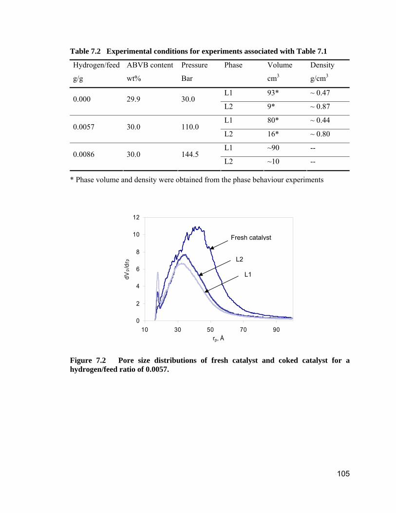
105
Table 7.2 Experimental conditions for experiments associated with Table 7.1
Hydrogen/feed
g/g
ABVB content
wt%
Pressure
Bar
Phase
Volume
cm3
Density
g/cm3
L1 93* ~ 0.47 0.000 29.9 30.0
L2 9* ~ 0.87
L1 80* ~ 0.44 0.0057 30.0 110.0
L2 16* ~ 0.80
L1 ~90 -- 0.0086 30.0 144.5
L2 ~10 --
* Phase volume and density were obtained from the phase behaviour experiments
0
2
4
6
8
10
12
10 30 50 70 90rp, Å
dVp /
drp
Figure 7.2 Pore size distributions of fresh catalyst and coked catalyst for a hydrogen/feed ratio of 0.0057.
Fresh catalyst
L2
L1
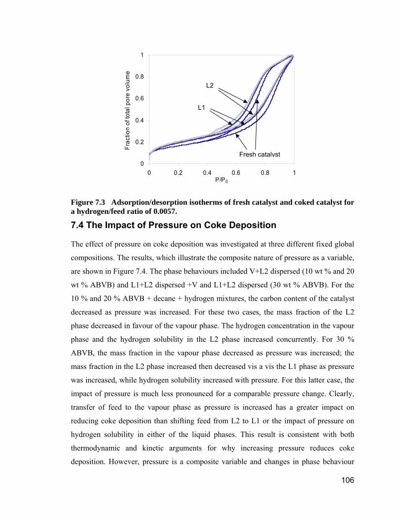
106
0
0.2
0.4
0.6
0.8
1
0 0.2 0.4 0.6 0.8 1P/P0
Frac
tion
of to
tal p
ore
volu
me
Figure 7.3 Adsorption/desorption isotherms of fresh catalyst and coked catalyst for a hydrogen/feed ratio of 0.0057.
7.4 The Impact of Pressure on Coke Deposition
The effect of pressure on coke deposition was investigated at three different fixed global
compositions. The results, which illustrate the composite nature of pressure as a variable,
are shown in Figure 7.4. The phase behaviours included V+L2 dispersed (10 wt % and 20
wt % ABVB) and L1+L2 dispersed +V and L1+L2 dispersed (30 wt % ABVB). For the
10 % and 20 % ABVB + decane + hydrogen mixtures, the carbon content of the catalyst
decreased as pressure was increased. For these two cases, the mass fraction of the L2
phase decreased in favour of the vapour phase. The hydrogen concentration in the vapour
phase and the hydrogen solubility in the L2 phase increased concurrently. For 30 %
ABVB, the mass fraction in the vapour phase decreased as pressure was increased; the
mass fraction in the L2 phase increased then decreased vis a vis the L1 phase as pressure
was increased, while hydrogen solubility increased with pressure. For this latter case, the
impact of pressure is much less pronounced for a comparable pressure change. Clearly,
transfer of feed to the vapour phase as pressure is increased has a greater impact on
reducing coke deposition than shifting feed from L2 to L1 or the impact of pressure on
hydrogen solubility in either of the liquid phases. This result is consistent with both
thermodynamic and kinetic arguments for why increasing pressure reduces coke
deposition. However, pressure is a composite variable and changes in phase behaviour
Fresh catalyst
L2
L1
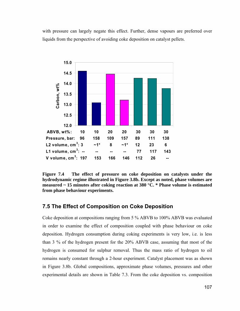
107
with pressure can largely negate this effect. Further, dense vapours are preferred over
liquids from the perspective of avoiding coke deposition on catalyst pellets.
12.0
12.5
13.0
13.5
14.0
14.5
15.0
10 10 20 20 30 30 30ABVB, wt%:
Car
bon,
wt%
Pressure, bar: 96 158 109 157 89 111 138 L2 volume, cm 3: 3 ~1* 8 ~1* 12 23 6L1 volume, cm 3: -- -- -- -- 77 117 143V volume, cm 3: 197 153 166 146 112 26 --
Figure 7.4 The effect of pressure on coke deposition on catalysts under the hydrodynamic regime illustrated in Figure 3.8b. Except as noted, phase volumes are measured ~ 15 minutes after coking reaction at 380 °C. * Phase volume is estimated from phase behaviour experiments.
7.5 The Effect of Composition on Coke Deposition
Coke deposition at compositions ranging from 5 % ABVB to 100% ABVB was evaluated
in order to examine the effect of composition coupled with phase behaviour on coke
deposition. Hydrogen consumption during coking experiments is very low, i.e. is less
than 3 % of the hydrogen present for the 20% ABVB case, assuming that most of the
hydrogen is consumed for sulphur removal. Thus the mass ratio of hydrogen to oil
remains nearly constant through a 2-hour experiment. Catalyst placement was as shown
in Figure 3.8b. Global compositions, approximate phase volumes, pressures and other
experimental details are shown in Table 7.3. From the coke deposition vs. composition
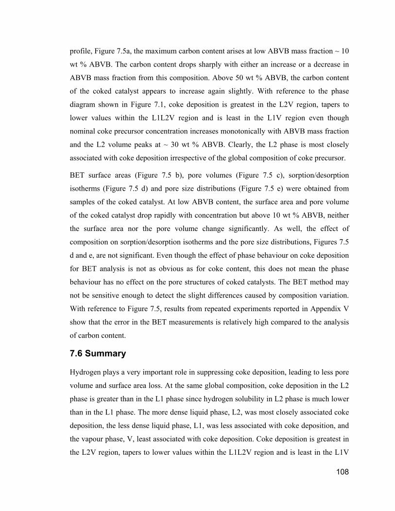
108
profile, Figure 7.5a, the maximum carbon content arises at low ABVB mass fraction ~ 10
wt % ABVB. The carbon content drops sharply with either an increase or a decrease in
ABVB mass fraction from this composition. Above 50 wt % ABVB, the carbon content
of the coked catalyst appears to increase again slightly. With reference to the phase
diagram shown in Figure 7.1, coke deposition is greatest in the L2V region, tapers to
lower values within the L1L2V region and is least in the L1V region even though
nominal coke precursor concentration increases monotonically with ABVB mass fraction
and the L2 volume peaks at ~ 30 wt % ABVB. Clearly, the L2 phase is most closely
associated with coke deposition irrespective of the global composition of coke precursor.
BET surface areas (Figure 7.5 b), pore volumes (Figure 7.5 c), sorption/desorption
isotherms (Figure 7.5 d) and pore size distributions (Figure 7.5 e) were obtained from
samples of the coked catalyst. At low ABVB content, the surface area and pore volume
of the coked catalyst drop rapidly with concentration but above 10 wt % ABVB, neither
the surface area nor the pore volume change significantly. As well, the effect of
composition on sorption/desorption isotherms and the pore size distributions, Figures 7.5
d and e, are not significant. Even though the effect of phase behaviour on coke deposition
for BET analysis is not as obvious as for coke content, this does not mean the phase
behaviour has no effect on the pore structures of coked catalysts. The BET method may
not be sensitive enough to detect the slight differences caused by composition variation.
With reference to Figure 7.5, results from repeated experiments reported in Appendix V
show that the error in the BET measurements is relatively high compared to the analysis
of carbon content.
7.6 Summary
Hydrogen plays a very important role in suppressing coke deposition, leading to less pore
volume and surface area loss. At the same global composition, coke deposition in the L2
phase is greater than in the L1 phase since hydrogen solubility in L2 phase is much lower
than in the L1 phase. The more dense liquid phase, L2, was most closely associated coke
deposition, the less dense liquid phase, L1, was less associated with coke deposition, and
the vapour phase, V, least associated with coke deposition. Coke deposition is greatest in
the L2V region, tapers to lower values within the L1L2V region and is least in the L1V
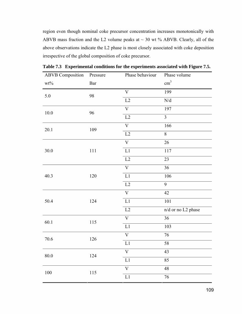
109
region even though nominal coke precursor concentration increases monotonically with
ABVB mass fraction and the L2 volume peaks at ~ 30 wt % ABVB. Clearly, all of the
above observations indicate the L2 phase is most closely associated with coke deposition
irrespective of the global composition of coke precursor.
Table 7.3 Experimental conditions for the experiments associated with Figure 7.5.
ABVB Composition
wt%
Pressure
Bar
Phase behaviour
Phase volume
cm3
V 199 5.0 98
L2 N/d
V 197 10.0 96
L2 3
V 166 20.1 109
L2 8
V 26
L1 117 30.0 111
L2 23
V 36
L1 106 40.3 120
L2 9
V 42
L1 101 50.4 124
L2 n/d or no L2 phase
V 36 60.1 115
L1 103
V 76 70.6 126
L1 58
V 43 80.0 124
L1 85
V 48 100 115
L1 76
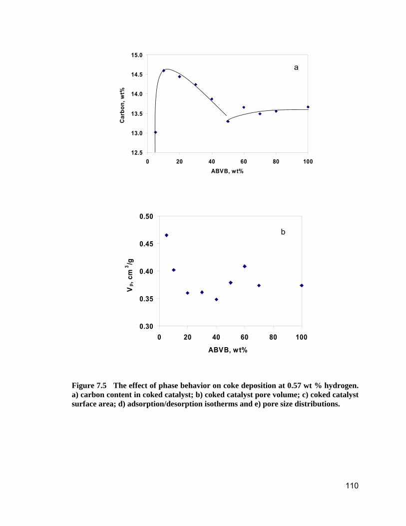
110
12.5
13.0
13.5
14.0
14.5
15.0
0 20 40 60 80 100ABVB, wt%
Car
bon,
wt%
0.30
0.35
0.40
0.45
0.50
0 20 40 60 80 100
ABVB, wt%
Vp,
cm3 /g
Figure 7.5 The effect of phase behavior on coke deposition at 0.57 wt % hydrogen. a) carbon content in coked catalyst; b) coked catalyst pore volume; c) coked catalyst surface area; d) adsorption/desorption isotherms and e) pore size distributions.
a
b
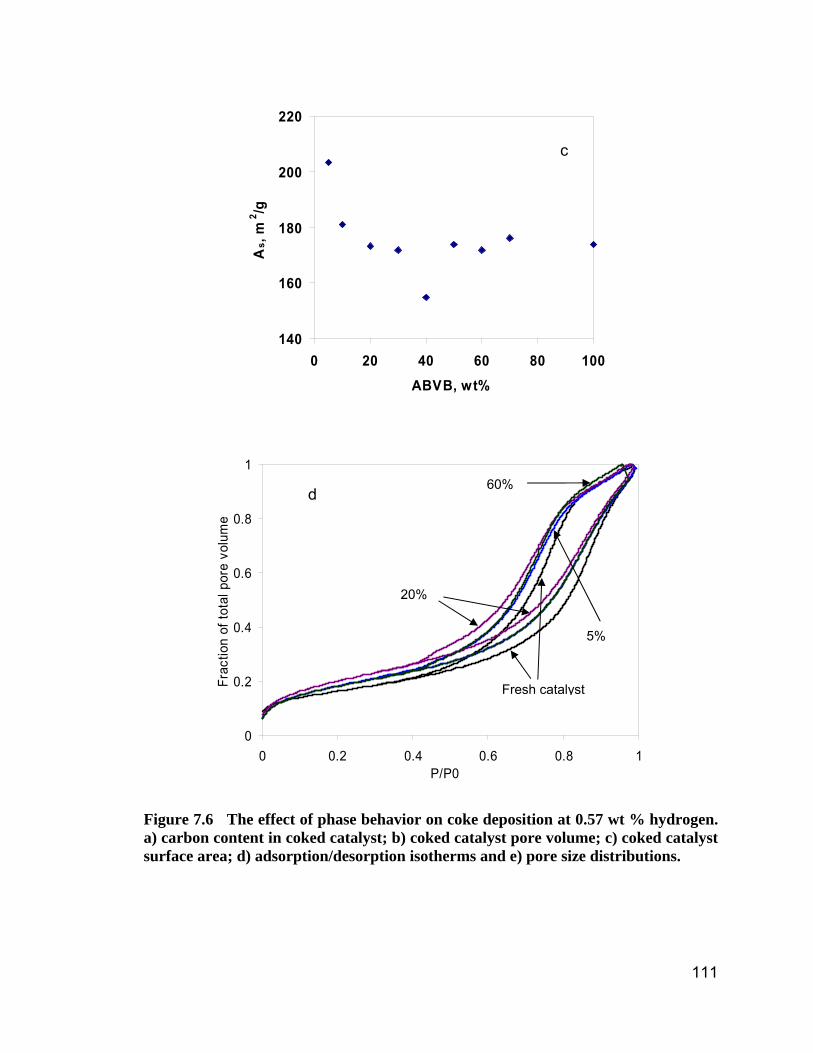
111
140
160
180
200
220
0 20 40 60 80 100ABVB, wt%
As,
m2 /g
0
0.2
0.4
0.6
0.8
1
0 0.2 0.4 0.6 0.8 1P/P0
Frac
tion
of to
tal p
ore
volu
me
Figure 7.6 The effect of phase behavior on coke deposition at 0.57 wt % hydrogen. a) carbon content in coked catalyst; b) coked catalyst pore volume; c) coked catalyst surface area; d) adsorption/desorption isotherms and e) pore size distributions.
Fresh catalyst
60%
20%
5%
c
d
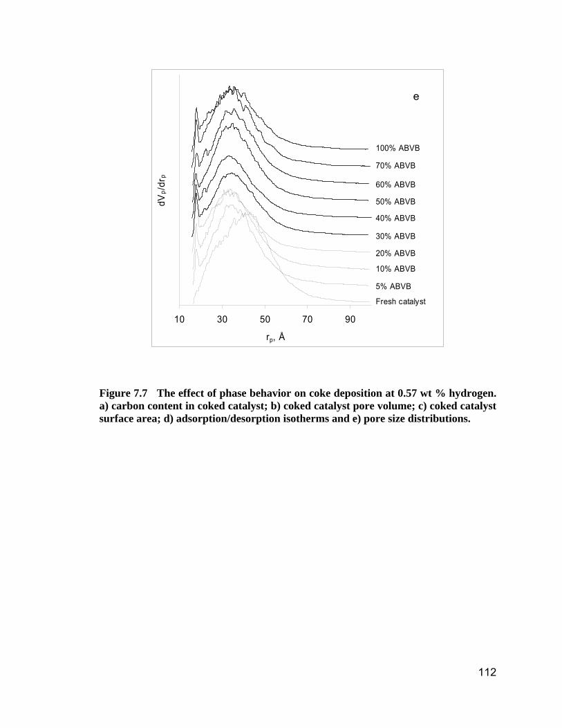
112
10 30 50 70 90
rp, Å
dVp/
drp
100% ABVB
70% ABVB
60% ABVB
50% ABVB
40% ABVB
30% ABVB
20% ABVB
10% ABVB
5% ABVB
Fresh catalyst
Figure 7.7 The effect of phase behavior on coke deposition at 0.57 wt % hydrogen. a) carbon content in coked catalyst; b) coked catalyst pore volume; c) coked catalyst surface area; d) adsorption/desorption isotherms and e) pore size distributions.
e
113
8. Coke Deposition Models
8.1 Coke Deposition Variation with Comparison
Development of quantitative models describing the rate of coke deposition on catalyst as
a function of coke precursors is frequently one of the aims of catalytic hydroprocessing
investigations. Such kinetic models are difficult to formulate. Coking kinetic equations,
whether based on empirical correlations or mechanistic models (Furimsky and Massoth,
1999; Froment and Bischoff, 1979), usually predict a smooth curve for coke deposition
versus coke precursor concentration for a fixed reaction time, temperature, and pressure.
If one assumes that an ABVB constituent is a coke precursor, the predicted coke
deposition profile should increase starting from a minimum, at 0 wt. % ABVB, to a
maximum at 100 percent ABVB in the feed. Catalyst coking experiments (batch reactor)
for 1-methyl naphthalene + ABVB + hydrogen mixtures appear to have exactly this trend
– Figure 8.1. The carbon content increases monotonically with ABVB content. From
previous work in our group, the 1-methly naphthalene + ABVB + hydrogen mixtures
exhibit only L1V phase behaviour. However, mixtures of decane + ABVB + hydrogen
exhibit complex multiphase behaviour under similar reaction conditions. The results from
the catalyst coking experiments (batch reactor) for decane + ABVB + hydrogen show a
pronounced maximum in the carbon content of the coked catalysts in the L2V phase
region at low ABVB concentration. The coke deposition profiles by view cell and batch
reactor have the same trend.
A sketch of coke deposition profiles, Figure 8.2, illustrates the difference between the
expected coke deposition profile and the profile observed in this work. The expected
profile follows the curve including segments I, III and II. The observed profile follows
curve segments I, IV and II. The two profiles overlap in segments I and II, i.e., in the V
and L1 or L1V phase regions and diverge for the L2V, L1L2V or L1L2 phase regions
(segment IV). This observed behaviour is inconsistent with expectation and with coke
deposition models where the extent of coke deposition, at otherwise fixed reaction
conditions, is proportional to the nominal concentration of coke precursor present in the
feed. The present results suggest that the nature of phases present must be included in
coke deposition models in order to capture key deposition phenomena. Coke deposition
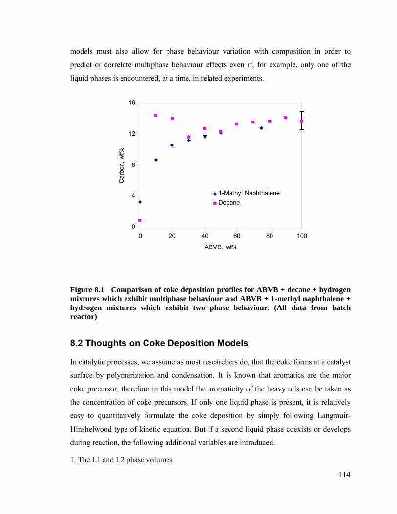
114
models must also allow for phase behaviour variation with composition in order to
predict or correlate multiphase behaviour effects even if, for example, only one of the
liquid phases is encountered, at a time, in related experiments.
0
4
8
12
16
0 20 40 60 80 100
ABVB, wt%
Car
bon,
wt%
1-Methyl NaphthaleneDecane
Figure 8.1 Comparison of coke deposition profiles for ABVB + decane + hydrogen mixtures which exhibit multiphase behaviour and ABVB + 1-methyl naphthalene + hydrogen mixtures which exhibit two phase behaviour. (All data from batch reactor)
8.2 Thoughts on Coke Deposition Models
In catalytic processes, we assume as most researchers do, that the coke forms at a catalyst
surface by polymerization and condensation. It is known that aromatics are the major
coke precursor, therefore in this model the aromaticity of the heavy oils can be taken as
the concentration of coke precursors. If only one liquid phase is present, it is relatively
easy to quantitatively formulate the coke deposition by simply following Langmuir-
Hinshelwood type of kinetic equation. But if a second liquid phase coexists or develops
during reaction, the following additional variables are introduced:
1. The L1 and L2 phase volumes
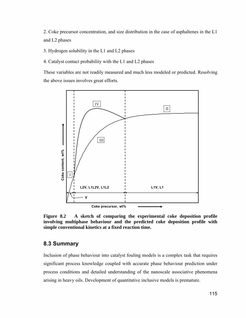
115
2. Coke precursor concentration, and size distribution in the case of asphaltenes in the L1
and L2 phases
3. Hydrogen solubility in the L1 and L2 phases
4. Catalyst contact probability with the L1 and L2 phases
These variables are not readily measured and much less modeled or predicted. Resolving
the above issues involves great efforts.
Coke precursor, wt%
Cok
e co
nten
t, w
t%
L1V, L1L2V, L1L2V, L1L2
V
III
IV II
I
Figure 8.2 A sketch of comparing the experimental coke deposition profile involving multiphase behaviour and the predicted coke deposition profile with simple conventional kinetics at a fixed reaction time.
8.3 Summary
Inclusion of phase behaviour into catalyst fouling models is a complex task that requires
significant process knowledge coupled with accurate phase behaviour prediction under
process conditions and detailed understanding of the nanoscale associative phenomena
arising in heavy oils. Development of quantitative inclusive models is premature.
116
9. Process Implications
9.1 Introduction
Based on the findings in this thesis, there are a number of implications for existing and
potential processes associated with petroleum refining processes. As the heavy liquid
phase causes more coke deposition, operators of existing processes should try to avoid
operating under conditions where the heavy liquid phase is present or to minimize the
amount of such phase; developers of new processes should select operating conditions
where heavy liquid phase formation is avoided. Specific process implications are
addressed below.
9.2 Trickle-Bed Reactor
Trickle-bed reactors are one of the most widely used reactor configurations in heavy oil
hydroprocessing. The reactor comprises a fixed bed of catalyst particles contacted by a
cocurrent downward gas-liquid flow carrying both reactants and products (Al-Dahhan et
al. 1997). According to the definition of trickle flow, the liquid flows down the column
from particle to particle on the surface of the catalyst particles while the gas phase flows
through the void space among the catalyst particles as shown in Figure 9.1a (Ng and Chu,
1987). From the coke deposition data presented here, over dilution of feeds with lighter
liquids or significant reaction leading to the production of lighter products, may push the
whole bed or the lower part of the bed from the L1V region into the L1L2V region.
Transfer to the L2V region would require significant dilution and is unlikely to arise in
industrial practice. If even a small mass fraction of the feed or the liquid in the reactor is
present as a dispersed L2 phase, then the flow regime and enhanced coke deposition
associated with the presence of L2 arises (Figure 9.1 b), and catalyst life is shortened.
The magnitude of this effect is uncertain at this time. From a practical perspective,
trickle-bed reactors for the hydroprocessing of heavy oils should be operated in the L1V
phase behaviour region to minimize coke deposition on catalyst. While dilution of heavy
feed is not normally practiced, it is important to note that such dilution employed in the
face of operating problems may exacerbate coke deposition for this application.
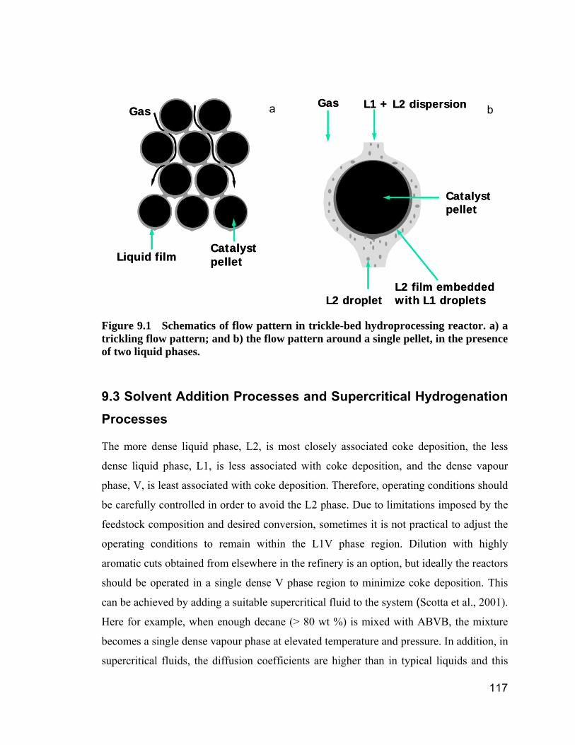
117
Figure 9.1 Schematics of flow pattern in trickle-bed hydroprocessing reactor. a) a trickling flow pattern; and b) the flow pattern around a single pellet, in the presence of two liquid phases.
9.3 Solvent Addition Processes and Supercritical Hydrogenation Processes
The more dense liquid phase, L2, is most closely associated coke deposition, the less
dense liquid phase, L1, is less associated with coke deposition, and the dense vapour
phase, V, is least associated with coke deposition. Therefore, operating conditions should
be carefully controlled in order to avoid the L2 phase. Due to limitations imposed by the
feedstock composition and desired conversion, sometimes it is not practical to adjust the
operating conditions to remain within the L1V phase region. Dilution with highly
aromatic cuts obtained from elsewhere in the refinery is an option, but ideally the reactors
should be operated in a single dense V phase region to minimize coke deposition. This
can be achieved by adding a suitable supercritical fluid to the system (Scotta et al., 2001).
Here for example, when enough decane (> 80 wt %) is mixed with ABVB, the mixture
becomes a single dense vapour phase at elevated temperature and pressure. In addition, in
supercritical fluids, the diffusion coefficients are higher than in typical liquids and this
Catalyst pellet
Gas L1 + L2 dispersion
L2 dropletL2 film embedded with L1 droplets
Catalyst pellet
Gas L1 + L2 dispersion
L2 dropletL2 film embedded with L1 droplets
Catalyst pellet
Gas
Liquid filmCatalyst pellet
Gas
Liquid film
a b
118
can enhance the desired hydrogenation reaction rates.
9.4 Summary
A practical approach to suppress coke deposition is by operating hydroprocessing
reactors in phase regions where no L2 phase exists. However, an optimized process
involves a lot of other considerations such as conversion rate, product qualities and so on.
Therefore, when a current process reaches its best optimization, the only way for
improvements is by modifying the current process or developing a new process. Solvent
addition process is an example of modification of previous conventional processes. By
fully understanding the new findings in this thesis from different perspectives, the current
industrial processes can be improved or new processes can be developed.
119
10. Conclusions
The impact of multiphase behaviour on coke deposition in commercial hydrotreating
catalyst pellets under typical catalytic hydrotreating conditions was explored using a
model heavy oil mixture. Prior to the catalyst coking experiments, the phase behaviour of
the model heavy oil system was first explored. The phase behaviour and catalyst coking
experiments were conducted both in the presence of hydrogen and in the absence of
hydrogen. The key conclusions are listed below:
1. The heavy oil model mixture Athabasca vacuum bottoms (ABVB) + decane exhibits
low-density liquid + vapour, L1V, high-density liquid + vapour, L2V, as well as low-
density liquid + high-density liquid + vapour, L1L2V, phase behaviour at typical
hydroprocessing conditions. This multiphase behaviour facilitates the study of the impact
of multiphase behaviour on coke deposition on NiMo/Al2O3 catalyst pellets.
2. As 380 °C is above the critical temperature of decane (344.6 °C), ABVB + decane
mixtures exhibit vapour phase behaviour at low ABVB mass fractions at this
temperature. For decane + 10, 20 wt % ABVB mixtures, L2 and L2V phase behaviour is
observed, depending on pressure. For decane + 70, 90, and 100 wt % ABVB mixtures,
only L1 and L1V phase behaviour was observed. L1L2V three phase equilibrium was
observed at intermediate compositions: 30, 35, 40, and 50 wt % ABVB. Phase behaviour
transitions from V for pure decane to L2V, to L1L2V, to L1V with increasing ABVB
content are readily observed.
3. The addition of hydrogen to ABVB + decane mixtures does not change the nature of
the phase behaviour significantly, but shifts the phase behaviour regions and boundaries
from lower pressures to higher pressures.
4. The catalyst coking experiments in the absence of hydrogen show that the carbon
content, surface area and pore volume losses for catalyst pellets exposed to the L1 phase
are greater than for the corresponding L2 cases despite a higher coke precursor
concentration in the L2 phase than in the L1 phase. This result may be attributed to
differences in the asphaltene aggregates size distribution and asphaltene solubility in
these two phases.
120
5. In the presence of hydrogen, the carbon content of the catalyst exposed to the L2 phase
is greater than for the corresponding L1 phase. Hydrogen solubility in the L1 phase is
greater than in the L2 phase. This facilitates hydrogenation preferentially in the L1 phase,
thus reducing coke deposition, as well as pore volume and surface area losses for catalyst
exposed to the L1 versus the L2 phase.
6. A comparison between experiments where no hydrogen is added and ones where it is
added shows that hydrogen solubility plays a very important role in suppressing coke
deposition in both L1 and L2 phases. And the hydrogen addition has a higher influence
on the L1 phase in coke suppression than on the L2 phase due to the higher hydrogen
solubility in L1 phase than in L2 phase.
7. In the presence of hydrogen, the more dense liquid phase, L2, was most closely
associated coke deposition, the less dense liquid phase, L1, was less associated with coke
deposition, and the vapour phase, V, is least associated with coke deposition.
8. Coke deposition is greatest in the L2V region, tapers to lower values within the L1L2V
region and is least in the L1V region even though nominal coke precursor concentration
increases monotonically with ABVB mass fraction and the L2 volume peaks at ~ 30 wt
% ABVB.
9. The results from catalyst coking experiments with decane + ABVB + hydrogen show
that the coke deposition variation with composition exhibits a maximum carbon content
in the L2V phase region. This observed result is inconsistent with expectation and with
coke deposition models where the extent of coke deposition, at otherwise fixed reaction
conditions, is proportional to the nominal concentration of coke precursor present in the
feed. The nature of phases present must be included in coke deposition models in order to
capture key deposition phenomena. Coke deposition models must also allow for phase
behaviour variation with composition in order to predict or correlate multiphase
behaviour effects even if, for example, only one of the liquid phases is encountered, at a
time, in experiments.
These findings have important implications for upgrading process development and
operation improvement even though the results negate some aspects of the hypothesis
proposed in Chapter 1. From a practical perspective, trickle-bed reactors for the

121
hydroprocessing of heavy oils should be operated in the L1V phase behaviour region to
minimize coke deposition on catalyst. Adding solvents with high solubility of heavy
hydrocarbons or supercritical fluids to heavy oil hydroprocessing reactors can also reduce
the coke deposition.
122
References
Abedi, S. J., “Unusual Retrograde Condensation and Asphaltene Precipitation in Model
Heavy Oil Systems Using X-ray Imaging”, PhD thesis, University of Toronto, 1998.
Abedi, S. J.; Seyfaie, S.; Shaw, J. M., “Unusual Retrograde Condensation and Asphaltene
Precipitation in a Model Heavy Oil System”, Petroleum Science and Technology, 16
(3&4), 209-226 (1998).
Absi-Halabi, M.; Stanislaus, A.; Trimm, D.L., “Coke Formation on Catalysts during the
Hydroprocessing of Heavy Oils”, Applied Catalysis, 72, 193-215 (1991).
Absi-Halabi, M.; Stanislaus, A.; Qabazard, H., “Trends in Catalysis Research to Meet
Future Refining Needs”, Hydrocarbon Processing, 76 (2), 45 (1997).
Al-Dahhan, M.H.; Larachi, F.; Dudukovic, M.P.; Laurent, A., “High-Pressure Trickle-
Bed Reactors: A Review”, Industrial & Engineering Chemistry Research, 36(8), 3292-
3314 (1997).
Ali, V., “The Impact of Phase Behaviour on Coke Formation in Delayed Cokers”, MSc
thesis, University of Toronto, 2002.
Amemiya, M.; Suzuka, T.; Korai, Y.; Mochida, I., “Catalyst Deactivation in Distillate
Hydrotreating (Part 1): Catalyst Deactivation in The Commercial Vacuum Gas Oil
Hydrotreating Unit”, Sekiyu Gakkaishi, 43(1), 52-58 (2000).
Asaoka, S.; Nakata, S.; Shiroto, Y.; Takeuchi, C. “Asphaltene Cracking in Catalytic
Hydrotreating of Heavy Oils. 2. Study of Changes in Asphaltene Structure during
Catalytic Hydroprocessing”, Industrial & Engineering Chemistry Process Design and
Development, 22, 242-248 (1983).
Baptist-Nguyen, S.; Subramanjam, B., “Coking and Activity of Porous Catalysts in
Supercritical Reaction Media”, AIChE Journal, 38(7), 1027-1037 (1992).
Bardon, C.; Barre, L.; Espinat, D.; Guille, V.; Li, M. H.; Lambard, J.; Ravey, J.C.;
Rosenberg, E.; Zemb, T., “The Colloidal Structure of Crude Oils and Suspensions of
Asphaltenes and Resins”, Fuel Science and Technology International, 14(1&2), 203-242
(1996).
123
Bartholdy, J.; Andersen, S. I., “Changes in Asphaltene Stability during Hydrotreating”,
Energy & Fuels, 14, 52-55 (2000).
Bartholdy, J.; Lauridsen, R.; Mejlholm, M.; Andersen, S. I., “Effect of Hydrotreatment on
Product Sludge Stability”, Energy & Fuels, 15, 1059-1062 (2001).
Bartholomew, C.H., “Catalyst Deactivation in Hydrotreating of Residua: A Review”, in:
M.C. Oballa, S.S. Shih (Eds.), Catalytic Hydroprocessing of Petroleum and Distillates,
Marcel Dekker, New York, 1994.
Beaton, W.I.; Bertolacini, R.J., “Resid Hydroprocessing at Amoco”, Catalysis Reviews-
Science and Engineering, 33 (3-4), 281-317 (1991).
Branco, V.A.M.; Mansoori, G.A.; Xavier, L.C.D.A.; Park, S.J. Manafi, H., “Asphaltene
Flocculation and Collapse from Petroleum Fluids”, Journal of Petroleum Science and
Engineering, 32, 217-230 (2001).
Butt, J.B.; Petersen, E.E., Activation, Deactivation, and Poisoning of Catalysts, Academic
Press Inc., San Diego, California, 1988, p 3-26.
Cai, H.Y.; Shaw, J.M.; Chung K.H., “Hydrogen Solubility Measurements in Heavy Oil
and Bitumen Cuts”, Fuel, 80(8), 1055-1063 (2001a).
Cai, H.Y.; Shaw, J. M.; Chung, K. H., “The Impact of Solid Additives on the Apparent
Solubility of Hydrogen in Petroleum Fractions and Model Hydrocarbon Liquids”, Fuel,
80, 1065-1077 (2001b).
Callejas, M.A.; Martínez, M.T.; Blasco, T.; Sastre, E., “Coke Charaterisation in Aged
Residue Hydrotreating Catalysts by Solid-State 13C-NMR Spectroscopy and
Temperatrue-Programmed Oxidation”, Applied Catalysis A: General, 218, 181-188
(2001).
Cartlidge, C. R.; Dukhedin-Lalla, L.; Rahimi, P.; Shaw, J. M., “Preliminary Phase
Diagrams for ABVB+n-Dodecane+Hydrogen”, Fluid Phase Equilibria, 117, 257-264
(1996).
Chang, H.J.; Seapan, M.; Crynes, B.L., “Catalyst Decay during Hydrotreatment of a
Heavy Coal Oil”, ACS Symposium Series, 196, 309-320 (1982).
124
Chung, K.H.; Xu, Chunming; Hu, Yunxiang; Wang, R., “Supercritical Fluid Extraction
Reveals Resid Properties”, Oil and Gas Journal, 95(3), 66-69 (1997).
Dautzenberg, F. M.; De Deken, J.C., “Modes of Operation in Hydrodemetallization”,
ACS symp. series 344, ACS, Washington, DC. 1987, p233-256.
Dautzenberg, F.M.; De Deken, J.C., “Reactor Developments in Hydrotreating and
Conversion of Residues”, Catalysis Reviews-Science and Engineering, 26 (3&4), 421-
444 (1984).
De Boer, D.K.G., “Fundamental Parameters for X-ray Fluorescence Analysis”
Spectrochimica Acta, 44B (11), 1171-1190 (1989).
De Jong, K.P.; Reinalda, D.; Emeis, C.A., “Coke Deposition in Trickle-Bed Reactors
during Heavy Oil Processing – Catalytic and Physical Effects”, Studies in Surface
Science and Catalysis, 88, 155-166 , Catalyst Deactivation (1994a).
De Jong, K.P. “Effects of Vapour-Liquid Equilibria on Coke Deposition in Trickle-Bed
Reactors during Heavy Oil Processing. 1. Experimental Results”, Industrial &
Engineering Chemistry Research, 33, 821-824 (1994b).
De Jong, K.P. “Effects of Vapor-Liquid Equilibria on Coke Deposition in Trickle-Bed
Reactors during Heavy Oil Processing. 2. Modeling”, Industrial & Engineering
Chemistry Research, 33, 3141-3145 (1994c).
Diez, F.; Gates, B.C.; Miller, J.T.; Sajkowski, D.J.; Kukes, S.G., “Deactivation of a Ni-
Mo/γ-Al2O3 Catalyst: Influence of Coke on the Hydroprocessing Activity, Industrial &
Engineering Chemistry Research, 29, 1999-2004 (1990).
Dukhedin-Lalla, L., “A Study of Complex Phase Behaviour Arising in Heavy Oil/
Bitumen Mixtures Using X-ray Imaging”, Ph.D. Thesis, University of Toronto, 1996.
Dukhedin-Lalla, L.; Sun, Y.S.; Shaw, J.M., “Phase Splitting of Complex Hydrocarbon
Mixtures”, Fluid Phase Equilibria, 53, 415-422 (1989).
Espinat, D.; Rosenberg, E.; Scarsella, M.; Barre, L.; Fenistein, D.; Broseta, D. “Colloidal
Structural Evolution from Stable to Flocculated State of Asphaltene Solutions and Heavy
Crudes”, in Mullins O.C.; Sheu, E.Y., Structures and Dynamics of Asphaltenes, Plenum
125
press, New York, 1998, p145-201.
Froment G.F.; Bischoff, K.B., Chemical Reactor Analysis and Design, John Wiley &
Sons: New York, 1979.
Furimsky, E., “Selection of Catalysts and Reactors for Hydroprocessing”, Applied
Catalysis A: General, 171, 177-206 (1998).
Furimsky, E.; Massoth, F.E., “Deactivation of Hydroprocessing Catalysts”, Catalysis
Today, 52, 381-495 (1999).
Gosselink, J.W.; van Veen, J.A.R., “Coping with Catalyst Deactivation in Hydrocarbon
Processing”, in Delmon B. and Froment, G.F. eds. Catalyst Deactivation, 1999, p3-16.
Gray, M.R., Upgrading Petroleum Residues and Heavy Oils, M. Dekker, New York,
1994.
Gray, M.R. and Masliyah, J.H., Extraction and Upgrading of Oil Sands Bitumen:
Intensive Short Course, Edmonton, Alberta. University of Alberta, 2004.
Gray M.R.; Zhao, Y; McKnight, C.M.; Komar, D.A.; Carruthers, J.D., “Coking of
Hydroprocessing Catalyst by Residue Fractions of Bitumen”, Energy & Fuels, 13, 1037-
1045 (1999).
Gregg, S. J.; Sing, K. S., Adsorption, Surface Area and Porosity; Academic Press:
London and New York, 1982.
Gregorowicz, J.; de Loos, T.W.; de Swaan Arons, J., “Liquid-Liquid-Vapour Phase
Equilibria in the System Ethane+ Propane+ Eicosane: Retrograde Behaviour of the
Heavy Liquid Phase”, Fluid Phase Equilibria, 84, 225-250 (1993).
Gualda, G.; Kasztelan, S., “Initial Deactivation of Residue Hydrodemetallization
Catalysts”, Journal of Catalysis, 161, 319-337 (1996).
Gualda, G.; Toulhoat, H., “Study of the Deactivation of Hydrotreating Catalysts by
Coking”, Revue De L Institut Francais du Petrole, 43(4), 567-594 (1988).
Hauser, A.; Stanislaus, A.; Marafi, A.; Al-Adwani, A., “Initial Coke Deposition on
Hydrotreating Catalysts. Part II. Structure Elucidation of Initial Coke on
Hydrodematallation Catalysts”, Fuel, 84 (2-3), 259-269 (2005).
126
Haynes Jr., H.W.; Leung, K., “Catalyst Deactivation by Pore Plugging and Active-Site
Poisoning Mechanisms”, Chemical Engineering Communications, 23 (1-3), 161-179
(1983).
Higashi, H.; Takahashi, T.; Kai, T., “Involvement of Asphaltene Decomposition in the
Rapid Deactivation of Hydrodesulfurization Catalysts under Conditions for Deep
Desulfurization of Atmospheric Residue”, Journal of the Japan Petroleum Institute, 47
(4), 297-302 (2004).
Hughes, R., Deactivation of Catalysts, Academic Press, Orlando, Florida, 1984, p 7-28.
Idei, K.; Takahashi, T.; Kai, T., “Effect of Coke and Metal Deposition on Catalyst
Deactivation at Early Stages of Resid Hydrodesulfurization Operation”, Journal of the
Japan Petroleum Institute, 45(5), 295-304 (2002).
Kanda, W.; Siu, I; Adjaye, J.; Nelson, A.E.; Gray, M.R., “Inhibition and Deactivation of
Dydrodenitrogenation (HDN) Catalysts by Narrow-Boiling Fractions of Athabasca Coker
Gas Oil”, Energy & Fuels, 18, 539-546 (2004).
Koyama, H.; Nagai, E.; Kumagai, H., “Catalyst Deactivation in Commercial Residue
Hydrodesulfurization”, Deactivation and Testing of Hydrocarbon-Processing Catalysts,
ACS Symposium Series 634, 1996.
Kressmann, S.; Morel, F.; Harle, V.; Kasztelan, S., “Recent Developments in Fixed-bed
Catalytic Residue Upgrading”, Catalysis Today, 43, 203-215 (1998).
Kubo, J.; Higashi, H.; Ohmoto, Y.; Arao, H., “The Additive Effects of Hydrogen-
Donating Hydrocarbons Derived from Petroleum in Hydrotreating of Heavy Oils”, Prepr.
ACS, 39(3), 416-421 (1994).
Kubo, J.; Higashi, H.; Ohmoto, Y.; Arao, H., “Heavy Oil Hydroprocessing with the
Addition of Hydrogen-Donating Hydrocarbons Derived from Petroleum”, Energy &
Fuels, 10, 474-481 (1996).
Le Page, J.F.; Chatila, S.G.; Davidson, M., Resid and Heavy oil Processing, Editions
Technip, Paris, 1992.
Lee, S. Y.; Seader, J. D.; Tsai, Chung H.; Massoth, F. E., “Restrictive Diffusion under
127
Catalytic Hydroprocessing Conditions”, Industrial & Engineering Chemistry Research,
30, 29-38 (1991a).
Lee, S. Y.; Seader, J. D.; Tsai, Chung H.; Massoth, F. E., “Solvent and Temperature
Effects on Restrictive Diffusion under Reaction Conditions”, Industrial & Engineering
Chemistry Research, 30, 607-613 (1991b).
Li, S. H.; Liu, C. G.; Que, G. H.; Liang, W. J.; Zhu, Y. J., “Colloidal Structures of Three
Chinese Petroleum Vacuum Residues”, Fuel, 75, 1025-1029 (1996).
Li, S.; Liu, C.; Que, G.; Liang, W.; Zhu, Y., “Phase Separation Behaviours and Their
Relations with Coke Formation in Thermal Reaction Systems of Vacuum Residue”,
Petroleum Science and Technology, 17(7&8), 693-709 (1999).
Maham, Y.; Chodakowski, M.G.; Zhang, X.H.; Shaw, J.M., “Asphaltene Phase Behavior:
Prediction at A Crossroads”, Fluid Phase Equilibria, 227, 177–182 (2005).
Mansoori, G.A., “Modeling of Asphaltene and Other Heavy Organic Depositions”,
Journal of Petroleum Science and Engineering, 17, 101-111 (1997).
Marafi, M.; Stanislaus, A., “Influence of Catalyst Acidity and Feedstock Quality on
Hydrotreating Catalyst Deactivation by Coke Deposition”, Petroleum Science and
Technology, 19(5&6), 697-710 (2001).
Matsushita, K.; Hauser, A.; Marafi, A.; Koide, R.; Stanislaus, A., “Initial Coke
Deposition on Hydrotreating Catalysts. Part 1. Changes in Coke Properties as a Function
of Time of Stream”, Fuel, 83, 1031–1038 (2004).
Matsushita, K.; Marafi, A.; Hauser, A.; Stanislaus, A., “Relation between Relative
Solubility of Asphaltenes in the Product Oil and Coke Deposition in Residue
Hydroprocessing”, Fuel, 83, 1669–1674 (2004).
McHugh, M.A.; Krukonis, V.J., Supercritical Fluid Extraction: Principles and Practice,
2nd ed. Boston : Butterworth-Heinemann, 1994.
Mckinney, J.d.; Stipanov, J., “Gulf HDS Handles Resids”, Hydrocarbon Processing, 50
(5), 97 (1971).
Minicucci, D., “The Impact of Liquid-Liquid-Vapour Phase Behaviour on Coke
128
Formation from Model Coke Precursors”, MSc thesis, University of Toronto, 2000.
Minicucci, D.; Zou, X.Y.; Shaw, J.M., “The Impact of Liquid-Liquid-Vapour Phase
Behaviour on Coke Formation from Model Coke Precursors”, Fluid Phase Equilibria,
194-197, 353-360 (2002).
Morgan, G., “An Energy Renaissance of Oil Sands Development”, World Energy, 4, 46-
53, (2001).
Morel, F.; Kressmann, S.; Harle, V.; Kasztelan, S., “Processes and Catalysts for
Hydrocracking of Heavy Oil and Residues”, in Froment, G.F.; Demon, B.; Grange, P.
editors, Hydrotreatment and Hydrocracking of Oil Fractions, 1997, p1-16.
Muegge, B. D.; Massoth, F. E., “Basic Studies of Deactivation of Hydrogenation
Catalysts with Anthracene”, Fuel Processing Technology, 29, 19-30, (1991).
Murgich, J.; Abanero, J.A.; Strausz, O.P., “Molecular Recognition in Aggregates Formed
by Asphaltene and Resin Molecules from the Athabasca Oil Sand”, Energy & Fuels,
13(2), 278-286 (1999).
Ng, K.M.; Chu, C.F., “Trickle-Bed Reactors”, Chemical Engineering Progress, 83(11),
55-63 (1987).
Niu, C.F., PhD thesis, Research Institute of Petroleum Processing, 2001.
Nowlan, V.J.; Srinivasan, N.S., “Control of Coke Formation from Hydrocracked
Athabasca Bitumen”, Fuel Science and Technology International, 14(1&2), 41-54 (1996).
Overfield, R.E.; Sheu, E.Y.; Sinha, S.K.; Liang, K.S., “SANS Study of Asphaltene
Aggregation”, Fuel Science & Technology International, 7 (5-6), 611-624 (1989).
Pollack, N.; Enick, R., “The Mapping of Three Phase Volumetric Behaviour of Pseudo-
Binary”, Fluid Phase Equilibria, 39, 325-332 (1988).
Prausnitz, J.M.; Lichtenthaler, R.N.; Edmundo Gomes de Azevedo, Molecular
Thermodynamics of Fluid-Phase Equilibria, Upper Saddle River, New Jersey, 1999.
Priyanto, S.; Mansoori, G.A.; Suwono, A., “Measurement of Property Relationships of
Nano-Structure Micelles and Coacervates of Asphaltene in a Pure Solvent”, Chemical
Engineering Science, 56, 6933–6939 (2001).
129
Qabazard, H.; Adarme, R.; Crynes, B.L., in: D.L. Trimm et al. (Eds.), Catalysts in
Petroleum Refining 1989, Elsevier, Amsterdam, 1990.
Quann, R.J.; Ware, R.A.; Hung, C.W.; Wei, J., “Catalytic Hydrodemetallation of
Petroleum”, Advances in Chemical Engineering, 14, 95-259 (1988).
Radosz, M., “Multiphase Behaviour of Supercritical Fluid Systems: Oil Solutions in
Light Hydrocarbon Solvents”, Industrial & Engineering Chemistry Research, 26, 2134-
2139 (1987).
Rahmani, S.; McCaffrey, W.; Elliott, J.A.W.; Gray, M.R., “Liquid-Phase Behaviour
during the Cracking of Asphaltenes”, Industrial & Engineering Chemistry Research, 42,
4101-4108 (2003).
Reynolds, J.G., “Effects of Asphaltene Precipitation on the Size of Vanadium-, Nickel-
and Sulfur-Containing Compounds in Heavy Crude Oils and Residua”, in Yen, T. F.;
Chilingarian, G.V. (eds), Asphaltenes and Asphalts, 1, Elsevier Science Press, New York,
1994.
Reynolds, J.G., “Metals and Heteroatoms in Heavy Oils” in Speight, J.G. (eds),
Petroleum Chemistry and Refining, Taylor& Francis Press, Washington DC, 1999.
Richardson, S. M.; Nagaishi, H.; Gray, M. R., “Initial Coke Deposition on a NiMo/γ-
Al2O3 Bitumen Hydrogenation Processing Catalyst”, Industrial & Engineering Chemistry
Research, 35, 3940-3950 (1996).
Robinson, D.B., “The Interface between Theory and Experiment”, Fluid phase Equilibria,
52, 1-14 (1989).
Sasaki, T.; Jenkins, R.G.; Eser, S.; Schobert, H.H., “Carbonization of Anthracene and
Phenanthrene. 1. Kinetics and Mesophase Development”, Energy & Fuels, 7(6), 1039-
1046 (1993).
Scheffer, B.; van Koten, M.A.; Robschlager, K.W.; de Boks, F.C., “The Shell Residue
Hydroconversion Process: Development and Achievements”, Catalysis Today, 43, 217-
224 (1998).
Scotta, D. S.; Radleinb, D.; Piskorzb, J.; Majerskib, P.; deBruijn, Th. J. W., “Upgrading
130
of Bitumen in Supercritical Fluids”, Fuel, 80(8), 1087-1099 (2001).
Seyer, F. A.; Gyte, C. W. AOSTRA Oilsands Handbook, Loren G. Hepler and Chu Hsi,
Eds. AOSTRA, 1989; Chapter 7: Viscosity.
Shaw, J.M., “A Correlation for Hydrogen Solubility in Alicyclic and Aromatic Solvents”,
The Canadian Journal of Chemical Engineering, 65, 293-298 (1987).
Shaw, J.M.; Gaikwad, R. P.; Stowe, D. A., “Phase Splitting of Pyrene-Tetralin Mixtures
under Coal Liquefaction Conditions”, Fuel, 67, 1554-1559 (1988).
Shaw, J.M., “Toward Common Generalized Phase Diagrams for Asphaltenes Containing
Hydrocarbon Fluids,” ACS Petroleum Chemistry Div. Preprints, 47 (4), 338-342 (2002).
Shaw, J.M.; de Loos, Th.W.; de Swaan Arons, J., “Prediction of Unusual Retrograde
Condensation in Model Reservoir Fluids”, Fluid Phase Equilibria, 84, 251-266 (1993).
Sheremata, J.M.; Gray, M.R.; Dettman, H.D.; McCaffrey, W.C., “Quantitative Molecular
Representation and Sequential Optimization of Athabasca Asphaltenes”, Energy & Fuels,
18 (5), 1377-1384 (2004).
Speight, J.G., The Chemistry and Technology of Petroleum, Marcel Dekker, New York,
1991.
Speight, J.G., “The Chemistry and Physics of Coking”, Korean Journal of Chemical
Engineering, 15(1), 1-8 (1998).
Speight, J.G., The Chemistry and Technology of Petroleum, New York, 1999.
Speight, J.G., The Desulfurization of Heavy Oils and Residua, Marcel Dekker, New
York, 2000.
Speight, J.G.; Ozum, B., Petroleum Refining Process, Marcel Dekker, New York, 2002.
Storm, D. A.; Barresi, R. J.; Sheu, E. Y., “Rheological Study of Ratawi Vacuum Residue
in the 298-673 K Temperature Range”, Energy & Fuels, 9, 168-176 (1995).
Storm, D. A.; Barresi, R. J.; Sheu, E. Y., “Flocculation of Asphaltenes in Heavy Oil at
Elevated Temperatures”, Fuel Science and Technology International, 14(1&2), 243-260
(1996).
131
Storm, D. A.; Barresi, R. J.; Sheu, E. Y.; Bhattacharya, A.K.; DeRosa, T.F., “Microphase
Behaviour of Asphaltic Micelles during Catalytic and Thermal Upgrading”, Energy &
Fuels, 12, 120-128 (1998).
Strausz, O.P.; Mojelsky, T.W.; Lown, E.M., “The Molecular Structure of Asphaltene - an
Unfolding Story”, Fuel, 71 (12), 1355-1363 (1992).
Takatsuka, T.; Kajiyama, R.; Kashimoto, H.; Matsuo, I.; Miwa, S., “A Practical Model of
Thermal Cracking of Residual Oil”, Journal of Chemical Engineering of Japan, 22, 304-
310 (1989).
Takeuchi, C.; Fukui, Y.; Nakamura, M.; Shiroto, Y., “Asphaltene Cracking in Catalytic
Hydrotreating of Heavy Oils. 1. Processing of Heavy Oils by Catalytic Hydroprocessing
and Solvent Deasphalting”, Industrial & Engineering Chemistry Process Design and
Development, 22, 236-242 (1983).
Ternan, M.; Furimsky, E.; Parsons, B.I., “Coke Formation of Hydrodesulfurization
Catalysts”, Fuel Processing Technology, 2, 45-55 (1979).
Ternan, M.; Rahimi, P.M.; Clugston, D.M.; Dettman, H.D., “The +525 C Residue before
and after Hydrocracking with Bimodal Catalysts of Varying Macropore Volume”, Energy
& Fuel, 8(3), 518-530 (1994).
Thakur, D.S.; Thomas, M.G., “Catalyst Deactivation in Heavy Petroleum and Synthetic
Crude Processing: A Review”, Applied Catalysis, 15, 197-225 (1985).
Trimm, D.L., “Catalyst Deactivation”, in: Absi-Halabi, M. et al. (eds), Catalysts in
Petroleum Refining and Petrochemical Industries, 1995.
Van Konynenburg, P.H.; Scott, R.L., “Critical Lines and Phase Equilibria in Binary van
der Waals Mixtures”, Philos. Trans. R. Soc. London, 298, 495-540 (1980).
Wiehe, I.A., “A solvent-Resid Phase Diagram for Tracking Resid Conversion”, Industrial
& Engineering Chemistry Research, 31(2), 530-536 (1992).
Wiehe, I.A., “A Phase-Separation Kinetic Model for Coke Formation”, Industrial &
Engineering Chemistry Research, 32(11), 2447-2454 (1993).
Wiehe, I.A., “The Pendant-Core Building Block Model of Petroleum Residua”, Energy &
132
Fuels, 8(3), 536-544 (1994).
Wilson, R.E.; Keith, P.C.; Haylett, R.E., “Liquid Propane: Use in Dewaxing,
Deasphalting, and Refining Heavy Oils”, Industrial and Engineering Chemistry, 28(9),
1065-1078 (1936).
Yanik S.J.; Frayer J.A.; Huling G.P.; Somers A.E., “Latest Data on Gulf HDS Process”,
Hydrocarbon Processing, 56 (5), 97-104 (1977).
Yen, T.F., “Asphaltenes: Types and Sources”, in Mullins O.C.; Sheu, E.Y.(eds),
Structures and Dynamics of Asphaltenes, Plenum press, New York, 1998, p145-201.
Zhao, S., Kotlyar, L.S., Woods, J.R., Sparks, B.D., Hardacre, K., Chung, K.H.,
“Molecular Transformation of Athabasca Bitumen End-Cuts during Coking and
Hydrocracking”, Fuel, 80, 1155–1163 (2001).
Zou, X.Y., “Selective Removal of Inorganic Fine Solids, Heavy Metals and Sulfur from
Bitumen/Heavy Oils”, PhD thesis, University of Toronto, 2003.
133
Appendix I. General Experimental Procedure Using X-ray View Cell
The following experimental procedure should be followed when experiments are conducted on the X-ray view cell apparatus:
1. Load the solid component; 2. Pressure test; 3. Vacuum test; 4. Load the liquid component; 5. Degas the system; 6. Load the gas component; 7. Preheat the sample; 8. Conduct formal experiment; 9. Discharge and dissemble
1. Load the solid component Following the installation instructions for the view cell assembly from the D.B. Robinson Company, install the view cell bottom cap, gaskets, beryllium insert and the Beryllium cylinder. Load all solid components and the magnetic stirrer into the view cell. Following the installation instructions for the view cell assembly from the D.B. Robinson Company, install the view cell top cap and seal it. (Refer to Beryllium X-ray View Cell Operating and Maintenance Guide, DB Robinson Design and Manufacturing Ltd. 1997) Start up the X-ray machine and the image system following their established procedures respectively. Make sure you can see a clear image on the TV and find the position of the bellows. 2. Pressure test
1. Open HV4 and HV8 to keep the pressure of both bellows side and view cell side identical; slowly open HV1, HV2 and HV3 and load the view cell with hydrogen until the pressure of view cell reaches over 10% higher than the maximum experimental pressure; close HV1, HV2 and HV3.
2. Use combustible gas detector to find the leaks and fix them. 3. After no leaks are detected with combustible gas detector, a 24-hrs pressure test is
performed. Before the long run of pressure test, record the temperature and
134
pressure of the view cell, and after 24 hrs later record the temperature and pressure of the view cell again and do necessary calculations to find any leakage.
4. Slowly switch HV9 to the vent position and release the gas inside the view cell to atmosphere.
3. Vacuum test
1. Switch HV9 and HV10 to the vacuum position. Turn on the vacuum pump and evacuate the view cell for 20 minutes and close HV9 and HV10. Record the temperature and pressure of the view cell.
2. Record the temperature and pressure of the view cell 24 hours later; do necessary calculations to find any vacuum leakage.
3. Find the leak and correct for it. 4. Load the liquid component
1. Close HV4 and HV8. 2. Use a clean syringe and weigh the desired amount of a liquid component; connect
the syringe to HV11. 3. Slowly open HV11 and HV12, and allow the liquid sample to be sucked into the
view cell; then close HV11 and HV12. 4. Open HV9 and HV10 to the vacuum position and vacuum evacuate the liquid and
solid components by turning on the vacuum pump; then close HV9 and HV10 after vacuum evacuation.
5. Degas the system
1. Heat the view cell up to 200 °C and keep constant temperature at 200 °C for 1 hour while turn on the stirrer as long as it is movable.
2. Cool down to room temperature; open HV4 and HV8, and switch HV9 and HV10 to vacuum position; turn on the vacuum pump to degas for 20 minutes.
Caution: Some light hydrocarbon solutions could be very volatile and poisonous. Safety precautions are mandatory. Also do not evacuate the view cell too long since it may result in imnegligible change to the sample composition due to the loss of volatile solvent. 6. Load the gas component
1. Open HV4 and HV8; then open HV1, HV2 and HV3 to load hydrogen into the system.
135
2. Close HV1, HV2, HV3, HV4 and HV8, and open HV9 to vent position; then slowly open HV8 until the bellows reaches the top of the view cell, but do not generate a pressure difference, then close HV8. Record the pressure and temperature and do the necessary calculation to check whether the mass of gas is equivalent to the expected value.
3. If more than the expected value, then release by slowly open HV4 and HV9; if lower than the expected value, then load the system to even higher pressure than before and repeat the step 1 to 3.
7. Preheat the sample Preheating is a key step to ensure consistent experimental data for the asphaltenes-containing heavy oil samples. Heavy oil sample, such as ABVB, are often solid or semi-solid, which make it very hard to completely mix with light hydrocarbon solvents at room temperatures. Besides Asphaltenes are prone to form aggregates in solution, and these aggregates need to be broken so that asphaltene “monomer” have sufficient opportunities to interact with solvent molecules. These problems are solved by preheating the asphaltenes-containing heavy oil. Typically in experiment, the heavy oil + light hydrocarbon solvent mixtures are heated to 300 °C and the mixer is switched to high speed and kept running for 30 minutes at this temperature. Turn off the heating system but keep the mixer on, and let the mixture cool down to room temperature. 8. Conduct formal experiment According to the experimental plan, conduct the formal experiment. During the formal experiment, all valves connecting to the view cell side should be closed. When there is a need to adjust the pressure of view cell, slowly open HV5, HV6, HV7 to load the nitrogen into the bellows if increasing the view cell pressure; slowly open HV8, HV9 to vent position to release the gas in the bellows if decreasing the view cell pressure. 9. Discharge and dissemble Cool down the view cell to room temperature. If the system pressure is higher than atmosphere, slowly release the gas in both bellows side and view cell side and always keep the bellows close to the top of the view cell by controlling the release rate of two sides and disconnect the tubing connecting the bellows first and plug the bellows side. If the system pressure is lower than atmosphere, disconnect the tubing connecting to the view cell side first to push the bellows up to the top of the view cell and plug the view cell side. Then disconnect another side and plug it. Dissemble the view cell and discharge

136
the sample. (Refer to Beryllium X-ray View Cell Operating and Maintenance Guide, DB Robinson Design and Manufacturing Ltd. 1997)
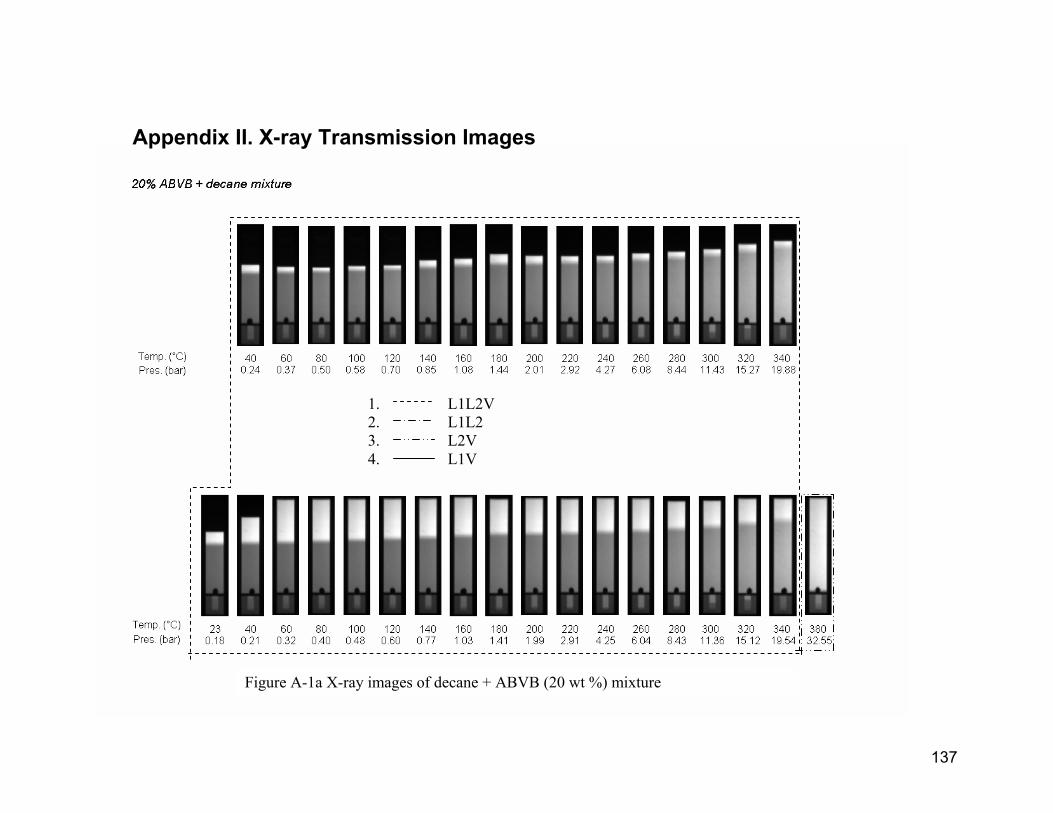
137
Figure A-1a X-ray images of decane + ABVB (20 wt %) mixture
Appendix II. X-ray Transmission Images
1. L1L2V 2. L1L2 3. L2V 4. L1V
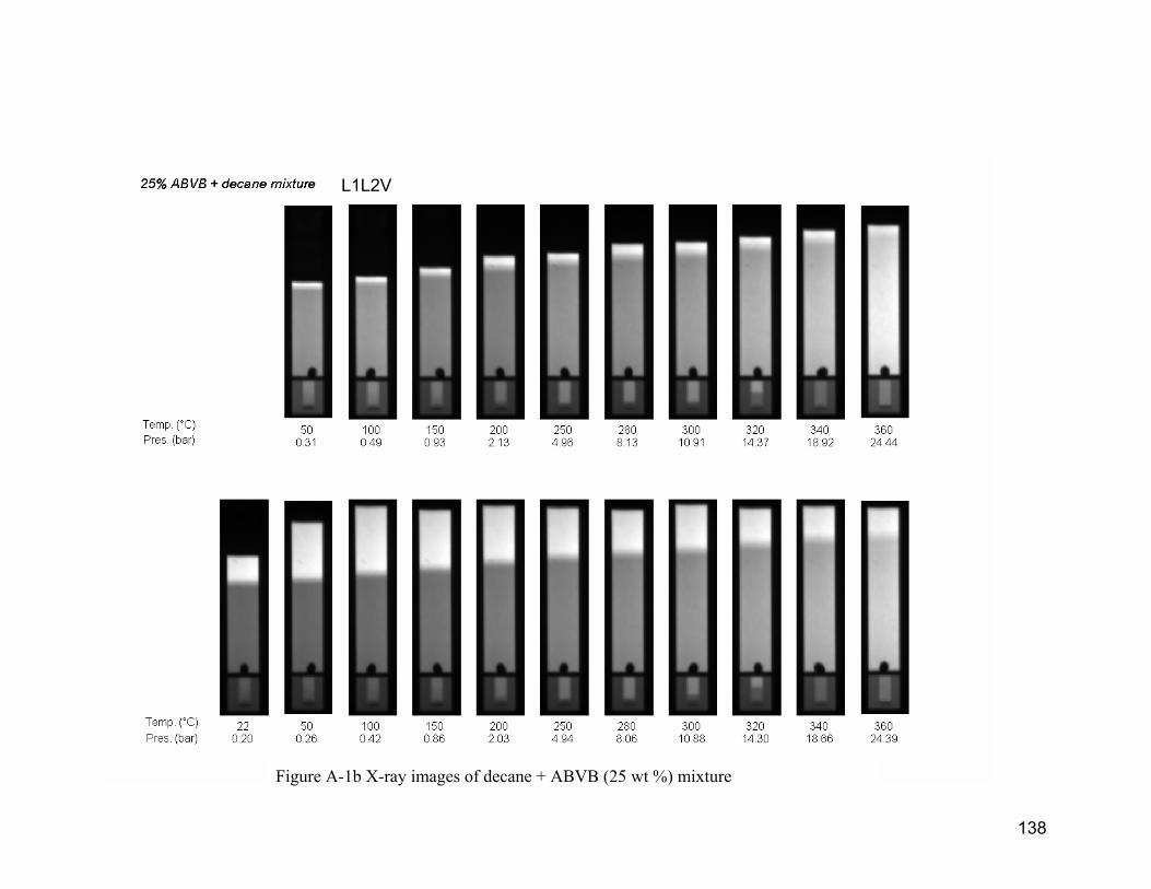
138
Figure A-1b X-ray images of decane + ABVB (25 wt %) mixture
L1L2V
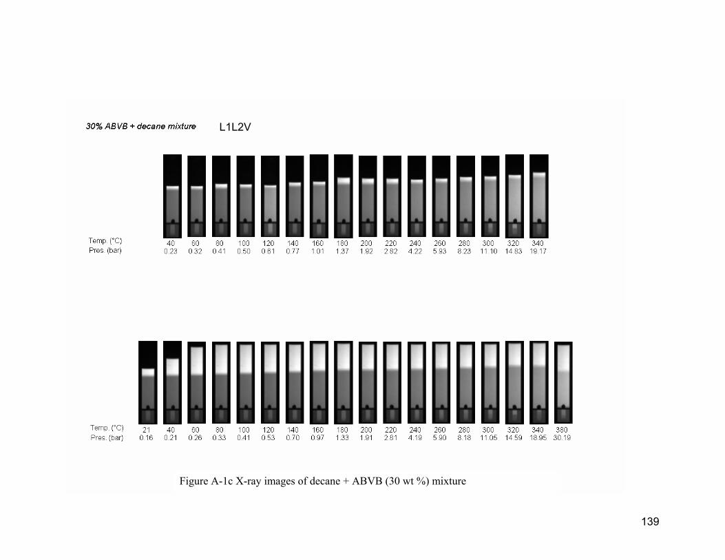
139
Figure A-1c X-ray images of decane + ABVB (30 wt %) mixture
L1L2V
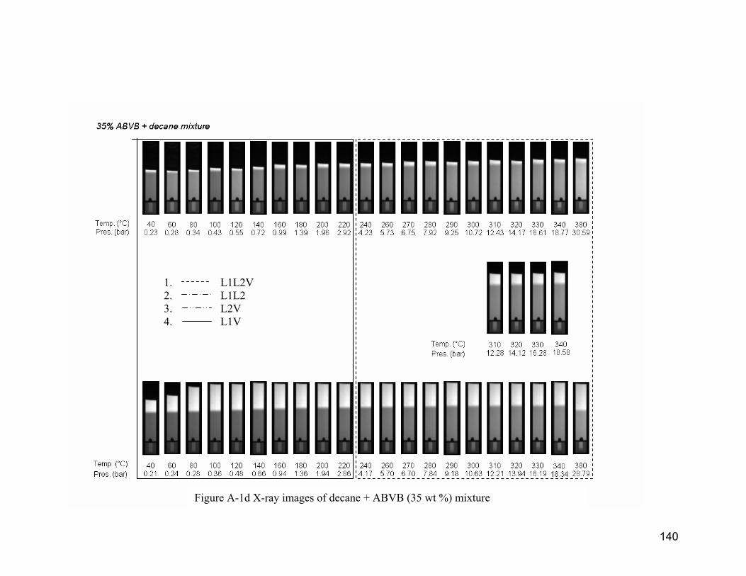
140
Figure A-1d X-ray images of decane + ABVB (35 wt %) mixture
1. L1L2V 2. L1L2 3. L2V 4. L1V
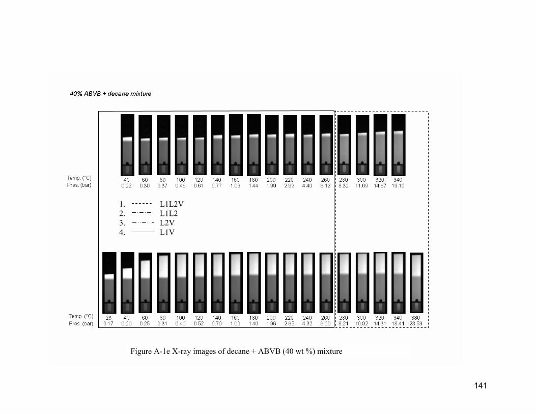
141
Figure A-1e X-ray images of decane + ABVB (40 wt %) mixture
1. L1L2V 2. L1L2 3. L2V 4. L1V
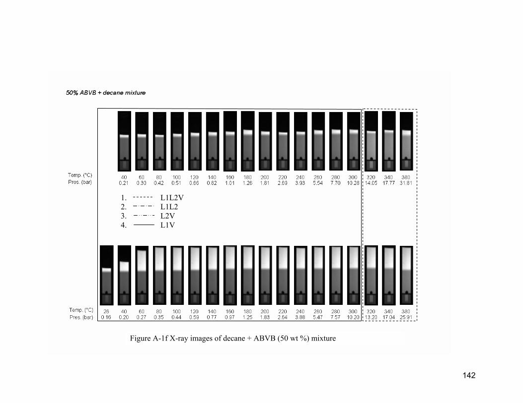
142
Figure A-1f X-ray images of decane + ABVB (50 wt %) mixture
1. L1L2V 2. L1L2 3. L2V 4. L1V

143
Figure A-1g X-ray images of decane + ABVB (70 wt %) mixture
L1V
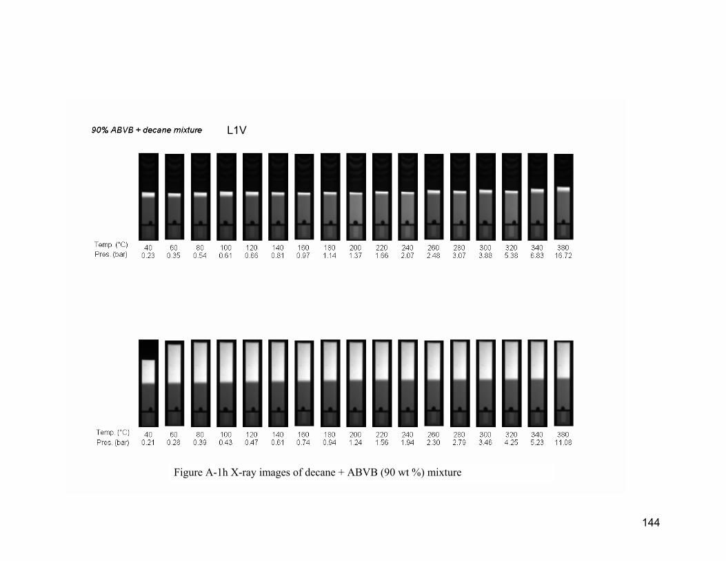
144
Figure A-1h X-ray images of decane + ABVB (90 wt %) mixture
L1V
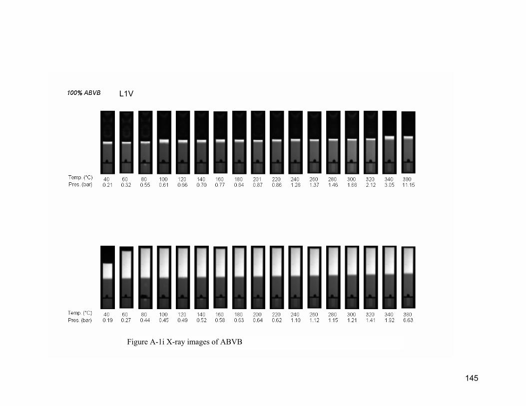
145
Figure A-1i X-ray images of ABVB
L1V
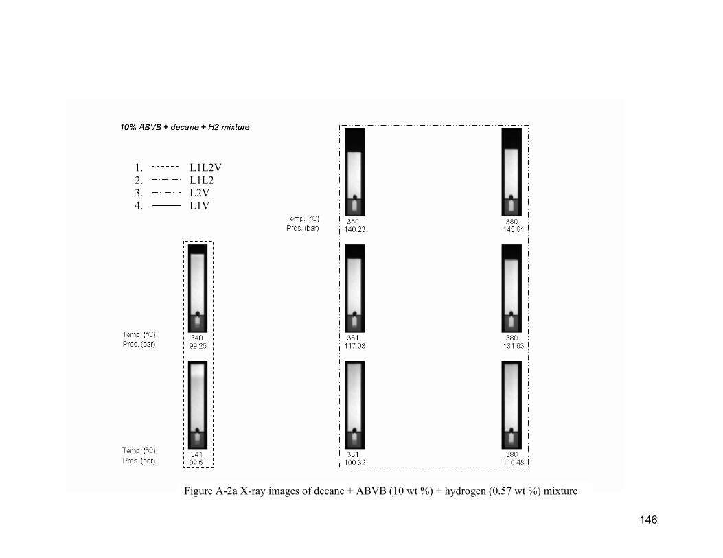
146
Figure A-2a X-ray images of decane + ABVB (10 wt %) + hydrogen (0.57 wt %) mixture
1. L1L2V 2. L1L2 3. L2V 4. L1V
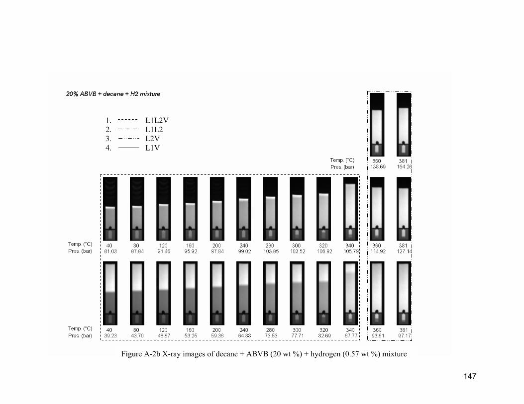
147
Figure A-2b X-ray images of decane + ABVB (20 wt %) + hydrogen (0.57 wt %) mixture
1. L1L2V 2. L1L2 3. L2V 4. L1V
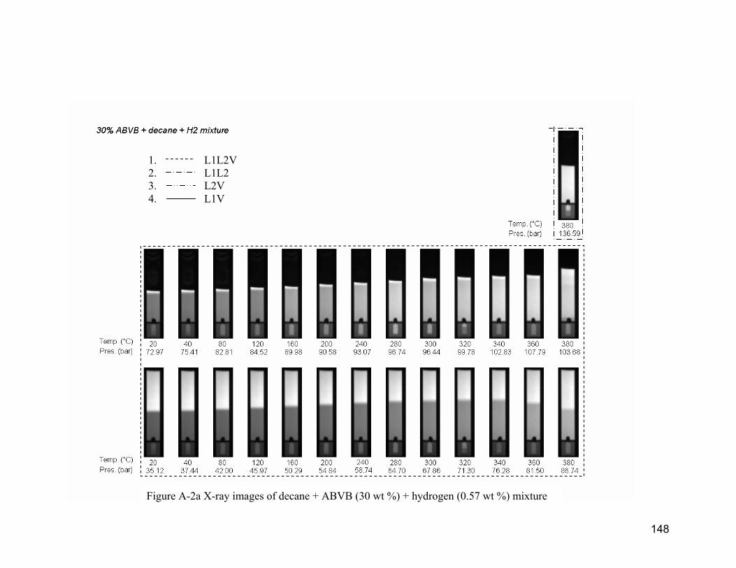
148
Figure A-2a X-ray images of decane + ABVB (30 wt %) + hydrogen (0.57 wt %) mixture
1. L1L2V 2. L1L2 3. L2V 4. L1V
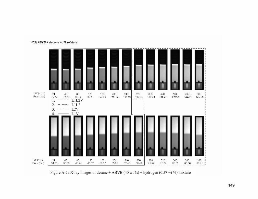
149
Figure A-2a X-ray images of decane + ABVB (40 wt %) + hydrogen (0.57 wt %) mixture
1. L1L2V 2. L1L2 3. L2V 4. L1V
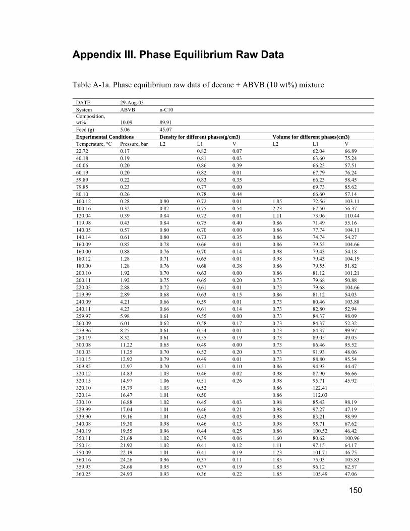
150
Appendix III. Phase Equilibrium Raw Data
Table A-1a. Phase equilibrium raw data of decane + ABVB (10 wt%) mixture
DATE 29-Aug-03 System ABVB n-C10 Composition, wt% 10.09 89.91 Feed (g) 5.06 45.07 Experimental Conditions Density for different phases(g/cm3) Volume for different phases(cm3) Temperature, °C Pressure, bar L2 L1 V L2 L1 V 22.72 0.17 0.82 0.07 62.04 66.89 40.18 0.19 0.81 0.03 63.60 75.24 40.06 0.20 0.86 0.39 66.23 57.51 60.19 0.20 0.82 0.01 67.79 76.24 59.89 0.22 0.83 0.35 66.23 58.45 79.85 0.23 0.77 0.00 69.73 85.62 80.10 0.26 0.78 0.44 66.60 57.14 100.12 0.28 0.80 0.72 0.01 1.85 72.56 103.11 100.16 0.32 0.82 0.75 0.54 2.23 67.50 56.37 120.04 0.39 0.84 0.72 0.01 1.11 73.06 110.44 119.98 0.43 0.84 0.75 0.40 0.86 71.49 55.16 140.05 0.57 0.80 0.70 0.00 0.86 77.74 104.11 140.14 0.61 0.80 0.73 0.35 0.86 74.74 54.27 160.09 0.85 0.78 0.66 0.01 0.86 79.55 104.66 160.00 0.88 0.76 0.70 0.14 0.98 79.43 54.18 180.12 1.28 0.71 0.65 0.01 0.98 79.43 104.19 180.00 1.28 0.76 0.68 0.38 0.86 79.55 51.82 200.10 1.92 0.70 0.63 0.00 0.86 81.12 101.21 200.11 1.92 0.75 0.65 0.20 0.73 79.68 50.88 220.03 2.88 0.72 0.61 0.01 0.73 79.68 104.66 219.99 2.89 0.68 0.63 0.15 0.86 81.12 54.03 240.09 4.21 0.66 0.59 0.01 0.73 80.46 103.88 240.11 4.23 0.66 0.61 0.14 0.73 82.80 52.94 259.97 5.98 0.61 0.55 0.00 0.73 84.37 98.09 260.09 6.01 0.62 0.58 0.17 0.73 84.37 52.32 279.96 8.25 0.61 0.54 0.01 0.73 84.37 99.97 280.19 8.32 0.61 0.55 0.19 0.73 89.05 49.05 300.08 11.22 0.65 0.49 0.00 0.73 86.46 95.52 300.03 11.25 0.70 0.52 0.20 0.73 91.93 48.06 310.15 12.92 0.79 0.49 0.01 0.73 88.80 95.54 309.85 12.97 0.70 0.51 0.10 0.86 94.93 44.47 320.12 14.83 1.03 0.46 0.02 0.98 87.90 96.66 320.15 14.97 1.06 0.51 0.26 0.98 95.71 45.92 320.10 15.79 1.03 0.52 0.86 122.41 320.14 16.47 1.01 0.50 0.86 112.03 330.10 16.88 1.02 0.45 0.03 0.98 85.43 98.19 329.99 17.04 1.01 0.46 0.21 0.98 97.27 47.19 339.90 19.16 1.01 0.43 0.05 0.98 83.21 98.99 340.08 19.30 0.98 0.46 0.13 0.98 95.71 67.62 340.19 19.55 0.96 0.44 0.25 0.86 100.52 46.42 350.11 21.68 1.02 0.39 0.06 1.60 80.62 100.96 350.14 21.92 1.02 0.41 0.12 1.11 97.15 64.17 350.09 22.19 1.01 0.41 0.19 1.23 101.71 46.75 360.16 24.26 0.96 0.37 0.11 1.85 75.03 105.83 359.93 24.68 0.95 0.37 0.19 1.85 96.12 62.57 360.25 24.93 0.93 0.36 0.22 1.85 105.49 47.06
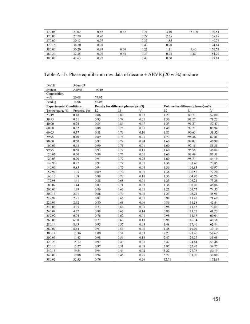
151
370.08 27.02 0.82 0.32 0.21 3.10 51.00 130.51 370.00 27.79 0.90 0.29 2.35 158.19 370.00 30.13 0.97 0.37 1.85 140.76 370.15 38.70 0.98 0.43 0.98 124.64 380.00 30.20 0.99 0.64 0.23 1.11 4.40 176.74 380.20 32.35 0.96 0.84 0.33 0.73 0.87 154.22 380.00 41.63 0.97 0.43 0.60 129.61
Table A-1b. Phase equilibrium raw data of decane + ABVB (20 wt%) mixture
DATE 5-Jun-03 System ABVB nC10 Composition, wt% 20.08 79.92 Feed, g 14.08 56.05 Experimental Conditions Density for different phases(g/cm3) Volume for different phases(cm3) Temperature, °C Pressure, bar L2 L1 V L2 L1 V 23.49 0.18 0.86 0.82 0.03 1.23 89.71 57.80 39.95 0.21 0.85 0.79 0.01 1.36 91.27 71.22 40.00 0.24 0.85 0.80 0.07 1.23 91.27 52.47 60.08 0.32 0.88 0.76 0.01 1.48 92.71 89.94 60.05 0.37 0.88 0.79 0.10 1.85 90.65 51.52 79.95 0.40 0.89 0.76 0.01 1.73 95.46 87.41 80.00 0.50 0.91 0.79 0.24 1.60 94.02 46.98 100.09 0.48 0.90 0.75 0.01 1.60 97.15 85.85 99.95 0.58 0.93 0.77 0.13 1.60 95.58 46.84 120.02 0.60 0.89 0.73 0.01 1.60 99.49 83.51 120.03 0.70 0.91 0.77 0.25 1.60 98.71 44.19 139.99 0.77 0.91 0.72 0.01 1.36 103.40 79.85 140.06 0.85 0.94 0.75 0.04 1.36 101.83 46.97 159.94 1.03 0.89 0.70 0.01 1.36 106.52 77.20 160.10 1.08 0.89 0.72 0.10 1.36 104.96 45.26 179.98 1.41 0.88 0.68 0.01 1.23 108.21 73.28 180.07 1.44 0.87 0.71 0.03 1.36 108.08 46.86 200.00 1.99 0.86 0.66 0.01 1.23 109.77 74.55 200.13 2.01 0.86 0.70 0.08 1.23 108.21 45.91 219.97 2.91 0.81 0.66 0.01 0.98 111.45 71.69 220.06 2.92 0.80 0.68 0.06 0.86 111.58 42.44 240.04 4.25 0.73 0.64 0.01 0.98 111.45 72.64 240.04 4.27 0.88 0.66 0.14 0.86 113.27 41.23 259.97 6.04 0.76 0.62 0.01 0.98 114.58 69.04 260.08 6.08 0.77 0.63 0.13 0.98 116.14 40.58 280.14 8.43 0.95 0.57 0.03 1.48 117.46 62.84 280.02 8.44 0.97 0.59 0.06 1.48 119.02 39.10 300.14 11.36 1.00 0.54 0.03 2.23 121.40 58.62 300.09 11.43 0.98 0.56 0.18 2.47 124.27 35.68 320.23 15.12 0.97 0.49 0.01 3.47 124.84 53.46 320.10 15.27 0.97 0.51 0.08 3.97 127.47 34.77 340.15 19.54 0.94 0.44 0.02 5.22 127.78 50.19 340.09 19.88 0.94 0.45 0.25 5.72 131.96 30.88 380.02 32.55 0.79 0.36 12.71 172.84

152
Table A-1c. Phase equilibrium raw data of decane + ABVB (30 wt%) mixture
DATE 12-Jun-03 System ABVB nC10 Composition, wt% 30.05 69.95 Feed, g 21.05 49.01 Experimental Conditions Density for different phases(g/cm3) Volume for different phases(cm3) Temperature, °C Pressure, bar L2 L1 V L2 L1 V 21.01 0.16 0.95 0.90 0.05 1.11 86.05 57.81 40.00 0.21 0.95 0.88 0.01 1.23 87.49 71.35 40.10 0.23 0.95 0.89 0.17 1.23 87.49 51.06 60.09 0.26 0.94 0.85 0.01 1.11 89.05 89.25 59.99 0.32 0.96 0.88 0.21 1.48 90.12 48.66 80.07 0.33 0.94 0.83 0.01 1.36 93.37 88.47 79.97 0.41 0.93 0.86 0.17 1.36 90.49 51.24 100.08 0.41 0.91 0.82 0.01 1.36 94.93 86.90 100.00 0.50 0.93 0.84 0.22 1.36 93.37 47.89 120.01 0.53 0.90 0.81 0.01 1.36 96.49 85.34 119.97 0.61 0.91 0.82 0.56 1.23 95.05 43.50 139.98 0.70 0.88 0.78 0.01 1.36 98.05 83.78 140.00 0.77 0.89 0.80 0.14 1.36 98.05 46.03 159.96 0.97 0.86 0.76 0.01 1.48 101.05 80.65 160.00 1.01 0.88 0.79 0.21 1.48 99.49 45.42 180.00 1.33 0.87 0.74 0.01 1.36 103.52 78.78 180.14 1.37 0.89 0.77 0.11 1.36 102.74 48.42 200.06 1.91 0.88 0.73 0.01 1.36 104.30 77.53 200.08 1.92 0.89 0.75 0.11 1.36 102.74 47.95 219.90 2.81 0.87 0.71 0.01 1.36 104.30 77.53 220.03 2.82 0.88 0.73 0.09 1.36 104.30 46.39 240.25 4.19 0.87 0.68 0.02 1.48 105.74 76.44 240.29 4.22 0.89 0.71 0.13 1.48 106.52 42.16 260.10 5.90 0.84 0.66 0.01 1.73 107.05 75.35 260.05 5.93 0.87 0.68 0.23 1.60 108.74 41.70 280.05 8.18 0.85 0.64 0.02 1.98 108.37 72.84 280.17 8.23 0.88 0.66 0.14 1.85 110.05 42.03 300.06 11.05 0.85 0.61 0.01 2.35 111.12 70.19 300.07 11.10 0.84 0.62 0.21 2.72 113.09 38.12 320.15 14.59 1.02 0.57 0.03 2.85 112.96 67.85 320.11 14.83 1.02 0.58 0.32 3.10 116.62 36.58 339.97 18.95 0.97 0.53 0.00 4.09 110.94 69.10 340.20 19.17 0.97 0.54 0.20 5.22 117.62 37.23 379.90 30.19 0.87 0.47 0.11 8.80 93.73 79.71
Table A-1d. Phase equilibrium raw data of decane + ABVB (35 wt%) mixture
DATE 31-Jul-03 System ABVB nC10 Composition, wt% 35.06 64.94 Feed, g 24.51 45.4 Experimental Conditions Density for different phases(g/cm3) Volume for different phases(cm3) Temperature, °C Pressure, bar L2 L1 V L2 L1 V 40.14 0.21 0.87 0.04 87.16 67.72 40.19 0.23 0.88 0.29 88.47 48.95 59.85 0.24 0.86 0.03 88.72 75.12 59.92 0.28 0.87 0.54 86.91 49.10 80.10 0.28 0.84 0.01 90.28 88.66
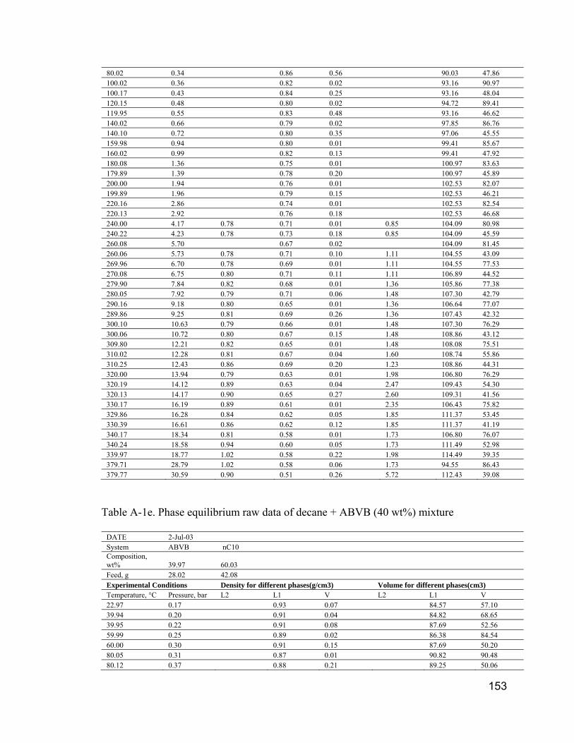
153
80.02 0.34 0.86 0.56 90.03 47.86 100.02 0.36 0.82 0.02 93.16 90.97 100.17 0.43 0.84 0.25 93.16 48.04 120.15 0.48 0.80 0.02 94.72 89.41 119.95 0.55 0.83 0.48 93.16 46.62 140.02 0.66 0.79 0.02 97.85 86.76 140.10 0.72 0.80 0.35 97.06 45.55 159.98 0.94 0.80 0.01 99.41 85.67 160.02 0.99 0.82 0.13 99.41 47.92 180.08 1.36 0.75 0.01 100.97 83.63 179.89 1.39 0.78 0.20 100.97 45.89 200.00 1.94 0.76 0.01 102.53 82.07 199.89 1.96 0.79 0.15 102.53 46.21 220.16 2.86 0.74 0.01 102.53 82.54 220.13 2.92 0.76 0.18 102.53 46.68 240.00 4.17 0.78 0.71 0.01 0.85 104.09 80.98 240.22 4.23 0.78 0.73 0.18 0.85 104.09 45.59 260.08 5.70 0.67 0.02 104.09 81.45 260.06 5.73 0.78 0.71 0.10 1.11 104.55 43.09 269.96 6.70 0.78 0.69 0.01 1.11 104.55 77.53 270.08 6.75 0.80 0.71 0.11 1.11 106.89 44.52 279.90 7.84 0.82 0.68 0.01 1.36 105.86 77.38 280.05 7.92 0.79 0.71 0.06 1.48 107.30 42.79 290.16 9.18 0.80 0.65 0.01 1.36 106.64 77.07 289.86 9.25 0.81 0.69 0.26 1.36 107.43 42.32 300.10 10.63 0.79 0.66 0.01 1.48 107.30 76.29 300.06 10.72 0.80 0.67 0.15 1.48 108.86 43.12 309.80 12.21 0.82 0.65 0.01 1.48 108.08 75.51 310.02 12.28 0.81 0.67 0.04 1.60 108.74 55.86 310.25 12.43 0.86 0.69 0.20 1.23 108.86 44.31 320.00 13.94 0.79 0.63 0.01 1.98 106.80 76.29 320.19 14.12 0.89 0.63 0.04 2.47 109.43 54.30 320.13 14.17 0.90 0.65 0.27 2.60 109.31 41.56 330.17 16.19 0.89 0.61 0.01 2.35 106.43 75.82 329.86 16.28 0.84 0.62 0.05 1.85 111.37 53.45 330.39 16.61 0.86 0.62 0.12 1.85 111.37 41.19 340.17 18.34 0.81 0.58 0.01 1.73 106.80 76.07 340.24 18.58 0.94 0.60 0.05 1.73 111.49 52.98 339.97 18.77 1.02 0.58 0.22 1.98 114.49 39.35 379.71 28.79 1.02 0.58 0.06 1.73 94.55 86.43 379.77 30.59 0.90 0.51 0.26 5.72 112.43 39.08
Table A-1e. Phase equilibrium raw data of decane + ABVB (40 wt%) mixture
DATE 2-Jul-03 System ABVB nC10 Composition, wt% 39.97 60.03 Feed, g 28.02 42.08 Experimental Conditions Density for different phases(g/cm3) Volume for different phases(cm3) Temperature, °C Pressure, bar L2 L1 V L2 L1 V 22.97 0.17 0.93 0.07 84.57 57.10 39.94 0.20 0.91 0.04 84.82 68.65 39.95 0.22 0.91 0.08 87.69 52.56 59.99 0.25 0.89 0.02 86.38 84.54 60.00 0.30 0.91 0.15 87.69 50.20 80.05 0.31 0.87 0.01 90.82 90.48 80.12 0.37 0.88 0.21 89.25 50.06
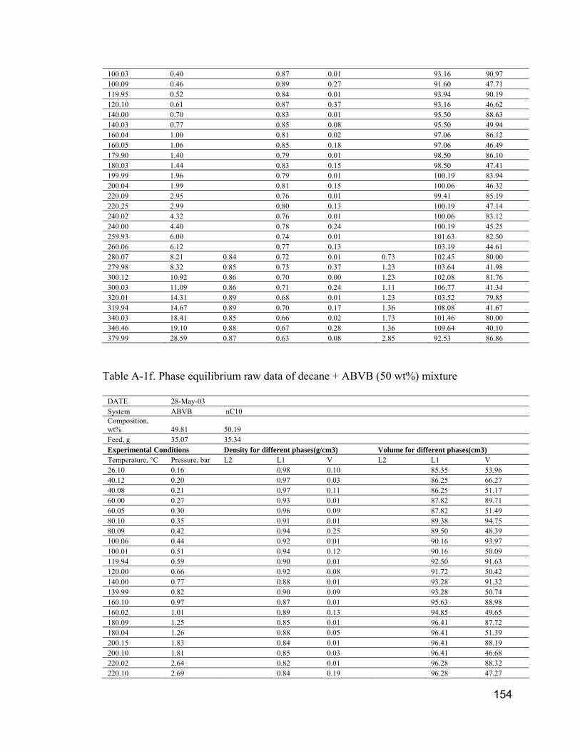
154
100.03 0.40 0.87 0.01 93.16 90.97 100.09 0.46 0.89 0.27 91.60 47.71 119.95 0.52 0.84 0.01 93.94 90.19 120.10 0.61 0.87 0.37 93.16 46.62 140.00 0.70 0.83 0.01 95.50 88.63 140.03 0.77 0.85 0.08 95.50 49.94 160.04 1.00 0.81 0.02 97.06 86.12 160.05 1.06 0.85 0.18 97.06 46.49 179.90 1.40 0.79 0.01 98.50 86.10 180.03 1.44 0.83 0.15 98.50 47.41 199.99 1.96 0.79 0.01 100.19 83.94 200.04 1.99 0.81 0.15 100.06 46.32 220.09 2.95 0.76 0.01 99.41 85.19 220.25 2.99 0.80 0.13 100.19 47.14 240.02 4.32 0.76 0.01 100.06 83.12 240.00 4.40 0.78 0.24 100.19 45.25 259.93 6.00 0.74 0.01 101.63 82.50 260.06 6.12 0.77 0.13 103.19 44.61 280.07 8.21 0.84 0.72 0.01 0.73 102.45 80.00 279.98 8.32 0.85 0.73 0.37 1.23 103.64 41.98 300.12 10.92 0.86 0.70 0.00 1.23 102.08 81.76 300.03 11.09 0.86 0.71 0.24 1.11 106.77 41.34 320.01 14.31 0.89 0.68 0.01 1.23 103.52 79.85 319.94 14.67 0.89 0.70 0.17 1.36 108.08 41.67 340.03 18.41 0.85 0.66 0.02 1.73 101.46 80.00 340.46 19.10 0.88 0.67 0.28 1.36 109.64 40.10 379.99 28.59 0.87 0.63 0.08 2.85 92.53 86.86
Table A-1f. Phase equilibrium raw data of decane + ABVB (50 wt%) mixture
DATE 28-May-03 System ABVB nC10 Composition, wt% 49.81 50.19 Feed, g 35.07 35.34 Experimental Conditions Density for different phases(g/cm3) Volume for different phases(cm3) Temperature, °C Pressure, bar L2 L1 V L2 L1 V 26.10 0.16 0.98 0.10 85.35 53.96 40.12 0.20 0.97 0.03 86.25 66.27 40.08 0.21 0.97 0.11 86.25 51.17 60.00 0.27 0.93 0.01 87.82 89.71 60.05 0.30 0.96 0.09 87.82 51.49 80.10 0.35 0.91 0.01 89.38 94.75 80.09 0.42 0.94 0.25 89.50 48.39 100.06 0.44 0.92 0.01 90.16 93.97 100.01 0.51 0.94 0.12 90.16 50.09 119.94 0.59 0.90 0.01 92.50 91.63 120.00 0.66 0.92 0.08 91.72 50.42 140.00 0.77 0.88 0.01 93.28 91.32 139.99 0.82 0.90 0.09 93.28 50.74 160.10 0.97 0.87 0.01 95.63 88.98 160.02 1.01 0.89 0.13 94.85 49.65 180.09 1.25 0.85 0.01 96.41 87.72 180.04 1.26 0.88 0.05 96.41 51.39 200.15 1.83 0.84 0.01 96.41 88.19 200.10 1.81 0.85 0.03 96.41 46.68 220.02 2.64 0.82 0.01 96.28 88.32 220.10 2.69 0.84 0.19 96.28 47.27
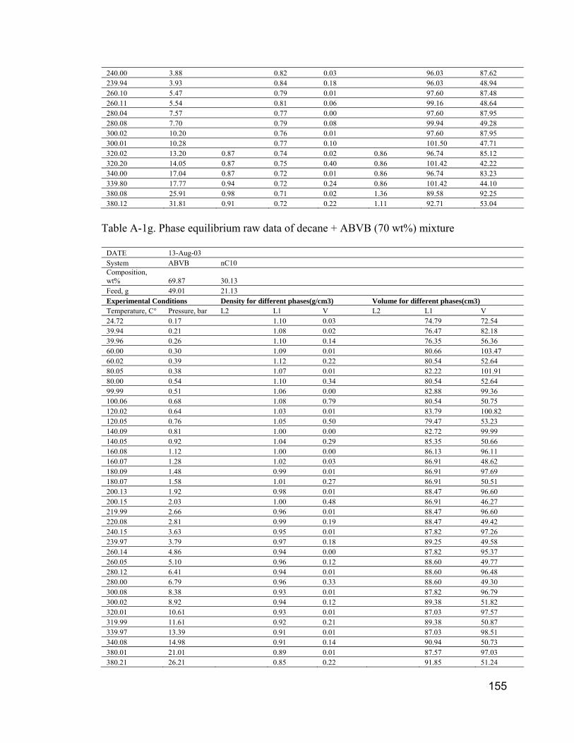
155
240.00 3.88 0.82 0.03 96.03 87.62 239.94 3.93 0.84 0.18 96.03 48.94 260.10 5.47 0.79 0.01 97.60 87.48 260.11 5.54 0.81 0.06 99.16 48.64 280.04 7.57 0.77 0.00 97.60 87.95 280.08 7.70 0.79 0.08 99.94 49.28 300.02 10.20 0.76 0.01 97.60 87.95 300.01 10.28 0.77 0.10 101.50 47.71 320.02 13.20 0.87 0.74 0.02 0.86 96.74 85.12 320.20 14.05 0.87 0.75 0.40 0.86 101.42 42.22 340.00 17.04 0.87 0.72 0.01 0.86 96.74 83.23 339.80 17.77 0.94 0.72 0.24 0.86 101.42 44.10 380.08 25.91 0.98 0.71 0.02 1.36 89.58 92.25 380.12 31.81 0.91 0.72 0.22 1.11 92.71 53.04
Table A-1g. Phase equilibrium raw data of decane + ABVB (70 wt%) mixture
DATE 13-Aug-03 System ABVB nC10 Composition, wt% 69.87 30.13 Feed, g 49.01 21.13 Experimental Conditions Density for different phases(g/cm3) Volume for different phases(cm3) Temperature, C° Pressure, bar L2 L1 V L2 L1 V 24.72 0.17 1.10 0.03 74.79 72.54 39.94 0.21 1.08 0.02 76.47 82.18 39.96 0.26 1.10 0.14 76.35 56.36 60.00 0.30 1.09 0.01 80.66 103.47 60.02 0.39 1.12 0.22 80.54 52.64 80.05 0.38 1.07 0.01 82.22 101.91 80.00 0.54 1.10 0.34 80.54 52.64 99.99 0.51 1.06 0.00 82.88 99.36 100.06 0.68 1.08 0.79 80.54 50.75 120.02 0.64 1.03 0.01 83.79 100.82 120.05 0.76 1.05 0.50 79.47 53.23 140.09 0.81 1.00 0.00 82.72 99.99 140.05 0.92 1.04 0.29 85.35 50.66 160.08 1.12 1.00 0.00 86.13 96.11 160.07 1.28 1.02 0.03 86.91 48.62 180.09 1.48 0.99 0.01 86.91 97.69 180.07 1.58 1.01 0.27 86.91 50.51 200.13 1.92 0.98 0.01 88.47 96.60 200.15 2.03 1.00 0.48 86.91 46.27 219.99 2.66 0.96 0.01 88.47 96.60 220.08 2.81 0.99 0.19 88.47 49.42 240.15 3.63 0.95 0.01 87.82 97.26 239.97 3.79 0.97 0.18 89.25 49.58 260.14 4.86 0.94 0.00 87.82 95.37 260.05 5.10 0.96 0.12 88.60 49.77 280.12 6.41 0.94 0.01 88.60 96.48 280.00 6.79 0.96 0.33 88.60 49.30 300.08 8.38 0.93 0.01 87.82 96.79 300.02 8.92 0.94 0.12 89.38 51.82 320.01 10.61 0.93 0.01 87.03 97.57 319.99 11.61 0.92 0.21 89.38 50.87 339.97 13.39 0.91 0.01 87.03 98.51 340.08 14.98 0.91 0.14 90.94 50.73 380.01 21.01 0.89 0.01 87.57 97.03 380.21 26.21 0.85 0.22 91.85 51.24
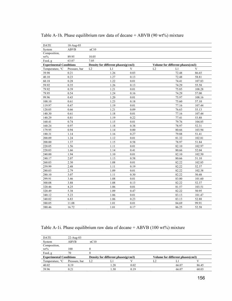
156
Table A-1h. Phase equilibrium raw data of decane + ABVB (90 wt%) mixture
DATE 18-Aug-03 System ABVB nC10 Composition, wt% 89.95 10.05 Feed, g 63.07 7.05 Experimental Conditions Density for different phases(g/cm3) Volume for different phases(cm3) Temperature, °C Pressure, bar L2 L1 V L2 L1 V 39.98 0.21 1.26 0.03 72.48 86.65 40.10 0.23 1.27 0.13 72.48 58.81 60.18 0.28 1.22 0.01 74.41 107.83 59.92 0.35 1.26 0.13 74.29 55.58 79.92 0.39 1.21 0.01 75.85 108.28 79.95 0.54 1.24 0.16 74.29 57.00 99.96 0.43 1.20 0.01 75.97 108.16 100.10 0.61 1.23 0.18 75.60 57.10 119.97 0.47 1.19 0.01 77.16 107.44 120.05 0.66 1.21 0.09 76.63 55.13 140.30 0.61 1.18 0.01 77.16 107.44 140.29 0.81 1.19 0.22 77.41 53.88 160.41 0.74 1.15 0.01 79.76 104.85 160.24 0.97 1.18 0.38 78.97 52.31 179.95 0.94 1.14 0.00 80.66 103.94 180.31 1.14 1.16 0.27 79.88 51.41 200.09 1.24 1.12 0.01 81.32 102.81 200.00 1.37 1.15 0.58 78.97 51.84 220.05 1.56 1.11 0.01 82.10 102.97 220.03 1.66 1.14 0.41 80.66 52.04 240.00 1.94 1.10 0.01 82.10 102.50 240.17 2.07 1.13 0.58 80.66 51.10 260.03 2.30 1.08 0.01 82.22 102.85 259.99 2.48 1.11 0.19 82.22 52.37 280.03 2.79 1.09 0.01 82.22 102.38 280.10 3.07 1.11 0.30 82.22 50.48 299.91 3.46 1.08 0.01 83.00 101.60 300.08 3.88 1.08 0.13 82.22 52.37 320.46 4.25 1.06 0.01 81.57 103.51 320.49 5.38 1.09 0.47 82.22 50.95 340.12 5.23 1.06 0.01 83.13 101.47 340.02 6.83 1.06 0.23 83.13 52.88 380.05 11.08 1.01 0.01 84.69 99.91 380.46 16.72 1.01 0.17 86.25 52.58
Table A-1i. Phase equilibrium raw data of decane + ABVB (100 wt%) mixture
DATE 22-Aug-03 System ABVB nC10 Composition, wt% 100 0 Feed, g 70 0 Experimental Conditions Density for different phases(g/cm3) Volume for different phases(cm3) Temperature, °C Pressure, bar L2 L1 V L2 L1 V 40.02 0.19 1.28 0.02 66.07 86.45 39.96 0.21 1.30 0.19 66.07 60.03
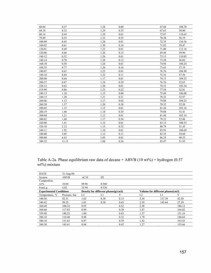
157
60.04 0.27 1.24 0.00 67.88 108.70 60.10 0.32 1.29 0.35 67.63 58.00 80.16 0.44 1.29 0.01 72.07 110.65 79.89 0.55 1.33 0.35 70.38 56.19 100.09 0.45 1.28 0.01 72.35 110.36 100.02 0.61 1.30 0.16 71.82 59.47 120.01 0.49 1.22 0.01 71.00 112.18 120.06 0.66 1.26 0.15 69.44 59.96 140.12 0.52 1.26 0.01 73.13 110.05 140.14 0.70 1.28 0.12 73.38 56.02 160.10 0.58 1.24 0.01 74.94 108.24 160.35 0.77 1.26 0.16 73.63 57.19 180.07 0.63 1.23 0.01 76.76 106.90 180.18 0.84 1.22 0.11 72.32 57.56 200.08 0.64 1.17 0.01 74.13 109.53 200.57 0.87 1.24 0.39 76.76 52.65 220.12 0.62 1.20 0.01 78.32 105.34 219.99 0.86 1.23 0.22 77.54 52.81 240.13 1.10 1.15 0.00 75.69 106.08 240.15 1.28 1.21 0.21 78.32 52.97 260.06 1.12 1.17 0.02 79.88 104.25 260.20 1.37 1.20 0.38 78.32 52.50 280.05 1.15 1.15 0.01 81.44 103.16 280.19 1.46 1.18 0.34 79.88 51.41 300.04 1.21 1.13 0.01 81.44 103.16 300.02 1.68 1.17 0.54 79.22 52.06 320.00 1.41 1.12 0.01 83.13 100.53 320.10 2.12 1.15 0.52 80.79 51.45 340.11 1.92 1.10 0.01 83.91 100.69 340.08 3.05 1.12 0.11 82.35 54.60 380.08 6.63 1.05 0.01 86.25 98.35 380.35 11.15 1.08 0.26 85.47 51.95
Table A-2a. Phase equilibrium raw data of decane + ABVB (10 wt%) + hydrogen (0.57 wt%) mixture
DATE 31-Aug-04 System ABVB nC10 H2 Compostion, wt% 10.04 89.96 0.560 Feed, g 6.02 53.94 0.336 Experimental Conditions Density for different phases(g/cm3) Volume for different phases(cm3) Temperature, °C Pressure, bar L2 L1 V L2 L1 V 340.56 92.51 1.02 0.38 0.15 2.39 137.39 42.50 340.42 99.25 1.01 0.38 0.43 2.39 143.64 27.29 360.68 100.32 0.95 0.32 2.58 180.12 360.60 117.03 0.99 0.38 1.87 164.82 359.98 140.23 1.00 0.43 1.57 151.16 380.10 110.48 0.98 0.32 1.79 180.64 380.10 131.63 0.97 0.39 1.42 163.43 380.30 145.61 0.94 0.42 1.27 155.66
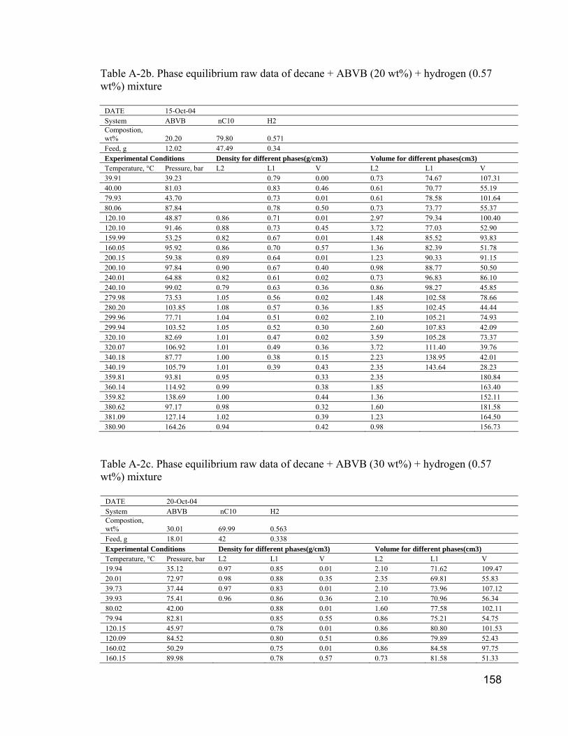
158
Table A-2b. Phase equilibrium raw data of decane + ABVB (20 wt%) + hydrogen (0.57 wt%) mixture
DATE 15-Oct-04 System ABVB nC10 H2 Compostion, wt% 20.20 79.80 0.571 Feed, g 12.02 47.49 0.34 Experimental Conditions Density for different phases(g/cm3) Volume for different phases(cm3) Temperature, °C Pressure, bar L2 L1 V L2 L1 V 39.91 39.23 0.79 0.00 0.73 74.67 107.31 40.00 81.03 0.83 0.46 0.61 70.77 55.19 79.93 43.70 0.73 0.01 0.61 78.58 101.64 80.06 87.84 0.78 0.50 0.73 73.77 55.37 120.10 48.87 0.86 0.71 0.01 2.97 79.34 100.40 120.10 91.46 0.88 0.73 0.45 3.72 77.03 52.90 159.99 53.25 0.82 0.67 0.01 1.48 85.52 93.83 160.05 95.92 0.86 0.70 0.57 1.36 82.39 51.78 200.15 59.38 0.89 0.64 0.01 1.23 90.33 91.15 200.10 97.84 0.90 0.67 0.40 0.98 88.77 50.50 240.01 64.88 0.82 0.61 0.02 0.73 96.83 86.10 240.10 99.02 0.79 0.63 0.36 0.86 98.27 45.85 279.98 73.53 1.05 0.56 0.02 1.48 102.58 78.66 280.20 103.85 1.08 0.57 0.36 1.85 102.45 44.44 299.96 77.71 1.04 0.51 0.02 2.10 105.21 74.93 299.94 103.52 1.05 0.52 0.30 2.60 107.83 42.09 320.10 82.69 1.01 0.47 0.02 3.59 105.28 73.37 320.07 106.92 1.01 0.49 0.36 3.72 111.40 39.76 340.18 87.77 1.00 0.38 0.15 2.23 138.95 42.01 340.19 105.79 1.01 0.39 0.43 2.35 143.64 28.23 359.81 93.81 0.95 0.33 2.35 180.84 360.14 114.92 0.99 0.38 1.85 163.40 359.82 138.69 1.00 0.44 1.36 152.11 380.62 97.17 0.98 0.32 1.60 181.58 381.09 127.14 1.02 0.39 1.23 164.50 380.90 164.26 0.94 0.42 0.98 156.73
Table A-2c. Phase equilibrium raw data of decane + ABVB (30 wt%) + hydrogen (0.57 wt%) mixture
DATE 20-Oct-04 System ABVB nC10 H2 Compostion, wt% 30.01 69.99 0.563 Feed, g 18.01 42 0.338 Experimental Conditions Density for different phases(g/cm3) Volume for different phases(cm3) Temperature, °C Pressure, bar L2 L1 V L2 L1 V 19.94 35.12 0.97 0.85 0.01 2.10 71.62 109.47 20.01 72.97 0.98 0.88 0.35 2.35 69.81 55.83 39.73 37.44 0.97 0.83 0.01 2.10 73.96 107.12 39.93 75.41 0.96 0.86 0.36 2.10 70.96 56.34 80.02 42.00 0.88 0.01 1.60 77.58 102.11 79.94 82.81 0.85 0.55 0.86 75.21 54.75 120.15 45.97 0.78 0.01 0.86 80.80 101.53 120.09 84.52 0.80 0.51 0.86 79.89 52.43 160.02 50.29 0.75 0.01 0.86 84.58 97.75 160.15 89.98 0.78 0.57 0.73 81.58 51.33
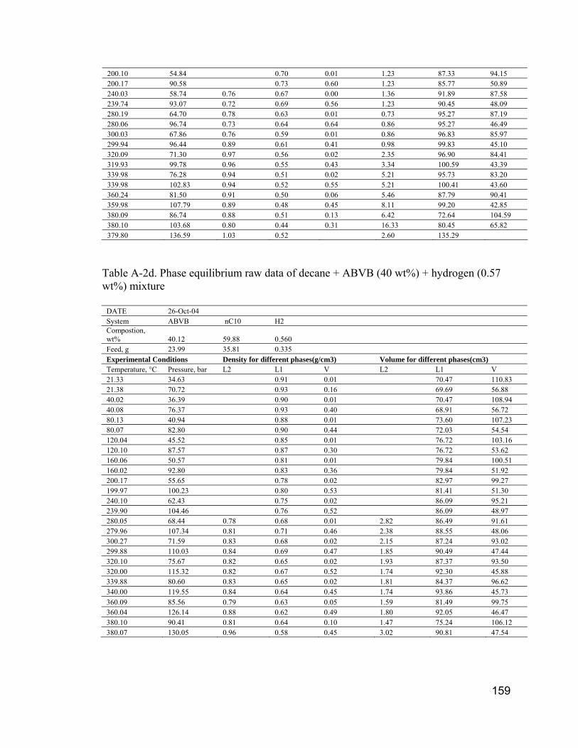
159
200.10 54.84 0.70 0.01 1.23 87.33 94.15 200.17 90.58 0.73 0.60 1.23 85.77 50.89 240.03 58.74 0.76 0.67 0.00 1.36 91.89 87.58 239.74 93.07 0.72 0.69 0.56 1.23 90.45 48.09 280.19 64.70 0.78 0.63 0.01 0.73 95.27 87.19 280.06 96.74 0.73 0.64 0.64 0.86 95.27 46.49 300.03 67.86 0.76 0.59 0.01 0.86 96.83 85.97 299.94 96.44 0.89 0.61 0.41 0.98 99.83 45.10 320.09 71.30 0.97 0.56 0.02 2.35 96.90 84.41 319.93 99.78 0.96 0.55 0.43 3.34 100.59 43.39 339.98 76.28 0.94 0.51 0.02 5.21 95.73 83.20 339.98 102.83 0.94 0.52 0.55 5.21 100.41 43.60 360.24 81.50 0.91 0.50 0.06 5.46 87.79 90.41 359.98 107.79 0.89 0.48 0.45 8.11 99.20 42.85 380.09 86.74 0.88 0.51 0.13 6.42 72.64 104.59 380.10 103.68 0.80 0.44 0.31 16.33 80.45 65.82 379.80 136.59 1.03 0.52 2.60 135.29
Table A-2d. Phase equilibrium raw data of decane + ABVB (40 wt%) + hydrogen (0.57 wt%) mixture
DATE 26-Oct-04 System ABVB nC10 H2 Compostion, wt% 40.12 59.88 0.560 Feed, g 23.99 35.81 0.335 Experimental Conditions Density for different phases(g/cm3) Volume for different phases(cm3) Temperature, °C Pressure, bar L2 L1 V L2 L1 V 21.33 34.63 0.91 0.01 70.47 110.83 21.38 70.72 0.93 0.16 69.69 56.88 40.02 36.39 0.90 0.01 70.47 108.94 40.08 76.37 0.93 0.40 68.91 56.72 80.13 40.94 0.88 0.01 73.60 107.23 80.07 82.80 0.90 0.44 72.03 54.54 120.04 45.52 0.85 0.01 76.72 103.16 120.10 87.57 0.87 0.30 76.72 53.62 160.06 50.57 0.81 0.01 79.84 100.51 160.02 92.80 0.83 0.36 79.84 51.92 200.17 55.65 0.78 0.02 82.97 99.27 199.97 100.23 0.80 0.53 81.41 51.30 240.10 62.43 0.75 0.02 86.09 95.21 239.90 104.46 0.76 0.52 86.09 48.97 280.05 68.44 0.78 0.68 0.01 2.82 86.49 91.61 279.96 107.34 0.81 0.71 0.46 2.38 88.55 48.06 300.27 71.59 0.83 0.68 0.02 2.15 87.24 93.02 299.88 110.03 0.84 0.69 0.47 1.85 90.49 47.44 320.10 75.67 0.82 0.65 0.02 1.93 87.37 93.50 320.00 115.32 0.82 0.67 0.52 1.74 92.30 45.88 339.88 80.60 0.83 0.65 0.02 1.81 84.37 96.62 340.00 119.55 0.84 0.64 0.45 1.74 93.86 45.73 360.09 85.56 0.79 0.63 0.05 1.59 81.49 99.75 360.04 126.14 0.88 0.62 0.49 1.80 92.05 46.47 380.10 90.41 0.81 0.64 0.10 1.47 75.24 106.12 380.07 130.05 0.96 0.58 0.45 3.02 90.81 47.54
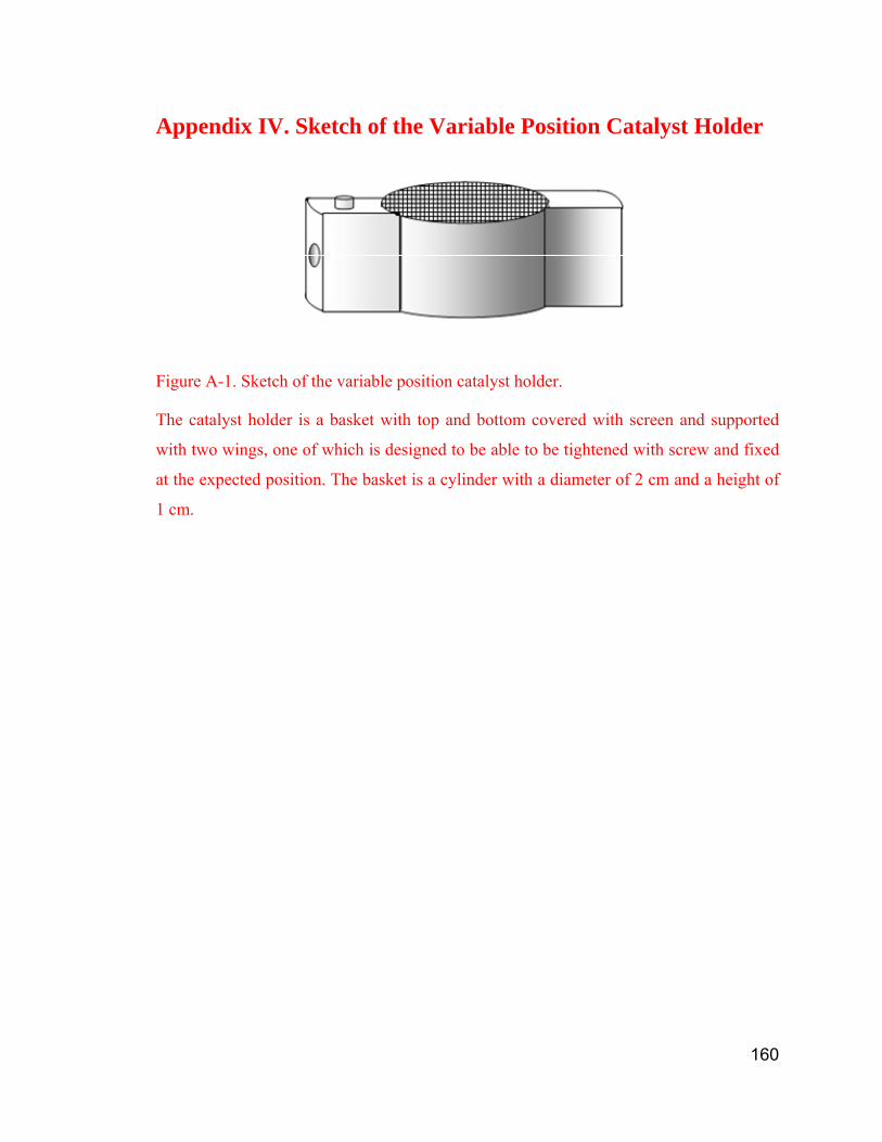
160
Appendix IV. Sketch of the Variable Position Catalyst Holder
Figure A-1. Sketch of the variable position catalyst holder.
The catalyst holder is a basket with top and bottom covered with screen and supported
with two wings, one of which is designed to be able to be tightened with screw and fixed
at the expected position. The basket is a cylinder with a diameter of 2 cm and a height of
1 cm.
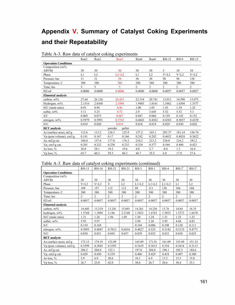
161
Appendix V. Summary of Catalyst Coking Experiments and their Repeatability
Table A-3. Raw data of catalyst coking experiments Run2 Run2 Run3 Run6 Run6 RH-12 RH-9 RH-15 Operation Conditions Composition (wt% ABVB) 30 30 30 30 30 5 10 10 Phase L1 L2 L1+L2 L1 L2 V+L2 V+L2 V+L2 Pressure, bar 31 31 29 30 30 98 96 158 Temperature, C 380 380 380 380 380 380 380 380 Time, hrs 5 5 5 2 2 2 2 2 H2/oil 0.0000 0.0000 0.0000 0.0000 0.0000 0.0057 0.0057 0.0057 Elmental analysis carbon, wt% 27.64 26.126 26.435 23.318 20.741 13.013 14.598 13.075 Hydrogen, wt% 2.1516 2.0368 2.1094 1.9403 1.8161 1.5462 1.6304 1.3577 H/C (mole ratio) 0.93 0.94 0.96 1.00 1.05 1.43 1.34 1.25 sulfur, wt% 5.11 5.25 4.72 2.9 3.645 5.52 5.52 5.3 S/C 0.069 0.075 0.067 0.047 0.066 0.159 0.142 0.152 nitrogen, wt% 0.5979 0.5991 0.5765 0.4843 0.4563 0.4383 0.5037 0.4239 N/C 0.019 0.020 0.019 0.018 0.019 0.029 0.030 0.028 BET analysis powder pellet As (surface area), m2/g 112.6 113.2 126.5 125.9 157.2 165.1 203.37 181.14 156.74 Vp (pore volume), cm3/g 0.141 0.167 0.17 0.166 0.242 0.292 0.4652 0.4024 0.3622 As, m2/g cat. 160.4 157.6 177.0 176.2 210.3 213.2 238.0 216.2 183.2 Vp, cm3/g cat. 0.201 0.232 0.238 0.232 0.324 0.377 0.544 0.480 0.423 As loss, % 26.8 28.1 19.2 19.6 4.0 2.7 -8.6 1.3 16.4 Vp loss, % 65.7 60.3 59.3 60.3 44.7 35.5 6.9 17.9 27.6
Table A-3. Raw data of catalyst coking experiments (continued)
RH-13 RH-14 RH-21 RH-21 RH-3 RH-1 RH-4 RH-21 RH-21 Operation Conditions Composition (wt% ABVB) 20 20 20 20 30 30 30 30 30 Phase V+L2 V+L2 V L2 L1+L2 L1+L2 L1+L2 L1 L2 Pressure, bar 109 157 112 112 89 111 138 104 104 Temperature, C 380 380 380 380 380 380 380 380 380 Time, hrs 2 2 2 2 2 2 2 2 2 H2/oil 0.0057 0.0057 0.0057 0.0057 0.0057 0.0057 0.0057 0.0057 0.0057 Elmental analysis carbon, wt% 14.445 13.219 13.241 15.691 14.261 14.236 13.76 14.64 16.35 hydrogen, wt% 1.5768 1.3894 2.146 2.2148 1.5423 1.4763 1.5033 1.5272 1.6678 H/C (mole ratio) 1.31 1.26 1.94 1.69 1.30 1.24 1.31 1.25 1.22 sulfur, wt% 5.93 5.97 3.94 3.26 3.95 4.68 4.83 S/C 0.154 0.169 0.104 0.086 0.108 0.120 0.111 nitrogen, wt% 0.5093 0.4847 0.7013 0.6816 0.4827 0.525 0.5142 0.5135 0.4771 N/C 0.030 0.031 0.045 0.037 0.029 0.032 0.032 0.030 0.025 BET analysis As (surface area), m2/g 173.15 174.19 152.09 165.89 171.91 161.09 155.49 151.33 Vp (pore volume), cm3/g 0.3599 0.3845 0.3393 0.3419 0.3613 0.354 0.3414 0.3113 As, m2/g cat. 206.2 204.0 152.1 197.0 204.0 190.1 185.5 184.6 Vp, cm3/g cat. 0.429 0.450 0.339 0.406 0.429 0.418 0.407 0.380 As loss, % 5.9 6.9 30.6 10.1 6.9 13.2 15.3 15.8 Vp loss, % 26.7 23.0 42.0 30.6 26.7 28.6 30.4 35.1
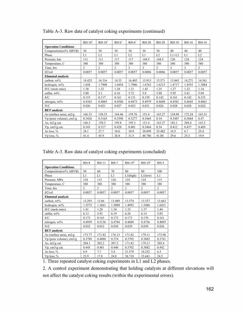
162
Table A-3. Raw data of catalyst coking experiments (continued)
RH-181 RH-181 RH-61 RH-61 RH-20 RH-20 RH-10 RH-16 RH-16 Operation Conditions Composition(wt% ABVB) 30 30 30 30 30 30 40 40 40 Phase L1 L2 L1 L2 L1 L2 L1+L2 L1 L2 Pressure, bar 111 111 117 117 144.5 144.5 120 124 124 Temperature, C 380 380 380 380 380 380 380 380 380 Time, hrs 2 2 2 2 2 2 2 2 2 H2/oil 0.0057 0.0057 0.0057 0.0057 0.0086 0.0086 0.0057 0.0057 0.0057 Elmental analysis carbon, wt% 14.425 16.316 14.35 16.405 13.915 15.571 13.865 14.271 14.561 hydrogen, wt% 1.658 1.7908 1.6454 1.7906 1.6763 1.6215 1.4717 1.4555 1.3884 H/C (mole ratio) 1.38 1.32 1.38 1.31 1.45 1.25 1.27 1.22 1.14 sulfur, wt% 5.88 5.1 6.16 5.72 5.9 5.88 5.95 5.41 5.94 S/C 0.153 0.117 0.161 0.131 0.159 0.142 0.161 0.142 0.153 nitrogen, wt% 0.4362 0.4065 0.4586 0.4473 0.4979 0.4688 0.4581 0.4645 0.4061 N/C 0.026 0.021 0.027 0.023 0.031 0.026 0.028 0.028 0.024 BET analysis As (surface area), m2/g 166.33 158.33 164.46 159.76 151.4 163.27 154.98 172.24 163.51 Vp (pore volume), cm3/g 0.3426 0.3165 0.3598 0.3277 0.3464 0.34 0.3487 0.3684 0.47 As, m2/g cat. 166.3 158.3 195.8 195.3 151.4 163.27 183.1 204.4 163.5 Vp, cm3/g cat. 0.343 0.317 0.428 0.401 0.3464 0.34 0.412 0.437 0.469 As loss, % 24.1 27.7 10.6 10.9 30.899 25.482 16.5 6.7 25.4 Vp loss, % 41.4 45.9 26.8 31.5 40.786 41.88 29.6 25.3 19.9
Table A-3. Raw data of catalyst coking experiments (concluded)
RH-8 RH-11 RH-7 RH-192 RH-192 RH-5 Operation Conditions Composition(wt% ABVB) 50 60 70 80 80 100 Phase L1 L1 L1 L1(high) L1(low) L1 Pressure, MPa 124 115 126 124 124 115 Temperature, C 380 380 380 380 380 380 Time, hrs 2 2 2 2 2 2 H2/oil 0.0057 0.0057 0.0057 0.0057 0.0057 0.0057 Elmental analysis carbon, wt% 13.293 13.66 13.489 13.574 13.537 13.663 hydrogen, wt% 1.5575 1.3661 1.5089 1.4992 1.5486 1.6431 H/C (mole ratio) 1.41 1.20 1.34 1.33 1.37 1.44 sulfur, wt% 6.13 5.92 6.19 6.26 6.14 5.85 S/C 0.173 0.163 0.172 0.173 0.170 0.161 nitrogen, wt% 0.4959 0.5136 0.4784 0.4609 0.4756 0.4095 N/C 0.032 0.032 0.030 0.029 0.030 0.026 BET analysis As (surface area), m2/g 173.77 171.82 176.13 171.82 179.11 173.96 Vp (pore volume), cm3/g 0.3789 0.4088 0.374 0.3702 0.3882 0.3741 As, m2/g cat. 204.1 202.2 207.2 171.82 179.11 205.4 Vp, cm3/g cat. 0.445 0.481 0.440 0.3702 0.3882 0.442 As loss, % 6.9 7.7 5.4 21.579 18.252 6.3 Vp loss, % 23.9 17.8 24.8 36.718 33.641 24.5
1. Three repeated catalyst coking experiments in L1 and L2 phases. 2. A control experiment demonstrating that holding catalysts at different elevations will not affect the catalyst coking results (within the experimental errors).
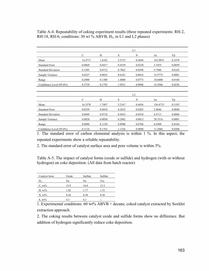
163
Table A-4. Repeatability of coking experiment results (three repeated experiments: RH-2, RH-18, RH-6; conditions: 30 wt % ABVB, H2, in L1 and L2 phases)
L1
C H S N As Vp
Mean 14.4717 1.6102 5.5733 0.4694 162.0933 0.3479
Standard Error 0.0869 0.0417 0.4539 0.0230 3.3455 0.0059
Standard Deviation 0.1505 0.0722 0.7862 0.0398 5.7946 0.0103
Sample Variance 0.0227 0.0052 0.6181 0.0016 33.5772 0.0001
Range 0.2900 0.1308 1.4800 0.0773 10.8400 0.0184
Confidence Level (95.0%) 0.3739 0.1792 1.9531 0.0988 14.3946 0.0256
L2
C H S N As Vp
Mean 16.3570 1.7497 5.2167 0.4436 156.4733 0.3185
Standard Error 0.0259 0.0410 0.2635 0.0205 2.6046 0.0048
Standard Deviation 0.0449 0.0710 0.4563 0.0354 4.5113 0.0084
Sample Variance 0.0020 0.0050 0.2082 0.0013 20.3516 0.0001
Range 0.0890 0.1230 0.8900 0.0706 8.4300 0.0164
Confidence Level (95.0%) 0.1116 0.1763 1.1336 0.0880 11.2066 0.0208
1. The standard error of carbon elemental analysis is within 1 %. In this aspect, the repeated experiments show a reliable repeatability. 2. The standard error of catalyst surface area and pore volume is within 3%. Table A-5. The impact of catalyst forms (oxide or sulfide) and hydrogen (with or without hydrogen) on coke deposition. (All data from batch reactor)
Catalyst form: Oxide Sulfide Sulfide
H2: No No Yes
C, wt% 15.9 16.0 13.3
H, wt% 1.82 1.77 1.31
N, wt% 0.36 0.38 0.36
S, wt% 4.3 6.1 --
1. Experimental conditions: 60 wt% ABVB + decane, coked catalyst extracted by Soxhlet extraction approach. 2. The coking results between catalyst oxide and sulfide forms show no difference. But addition of hydrogen significantly reduce coke deposition.
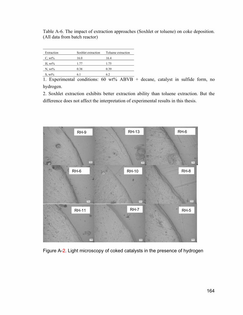
164
Table A-6. The impact of extraction approaches (Soxhlet or toluene) on coke deposition. (All data from batch reactor)
Extraction Soxhlet extraction Toluene extraction
C, wt% 16.0 16.4
H, wt% 1.77 1.75
N, wt% 0.38 0.39
S, wt% 6.1 6.2
1. Experimental conditions: 60 wt% ABVB + decane, catalyst in sulfide form, no hydrogen. 2. Soxhlet extraction exhibits better extraction ability than toluene extraction. But the difference does not affect the interpretation of experimental results in this thesis.
Figure A-2. Light microscopy of coked catalysts in the presence of hydrogen
RH-9 RH-13 RH-6
RH-6 RH-10 RH-8
RH-11 RH-7 RH-5
Recommended