WORKING PAPERS
THE IMPACT OF AUTOMOBILE FUEL ECONOMY STANDARDS
Andrew N. Kleit
WORKING PAPER NO. 160
February 1988
FiC Burean of Ecooomics working papers are preliminary materials circulated to stimulate discussion and critical commeot All data cootained in them are in the pnblic domaio. This includes infonnation obtained by the CommiSliioo which has become part of pnblic record. The analyses and conclnsions set forth are those of the anthors 8IId do not necessarily reflect the views of other members of the Burean of Economics, other Commissioo staff, or the Commission itself. Upon request, single copies of the paper will be provided. References in publications to FTC Bureau of Economics working papers by FTC economists (other than acknowledgement by a writer that he has access to such unpublished materials) should be cleared with the author to protect the teotative character of these papers.
BUREAU OF ECONOMICS FEDERAL TRADE COMMISSION
WASIllNGTON, DC 20580
The Impact of Automobile
Fuel Economy Standards
Andrew N. Kleit
Federal Trade Commission
The views presented here are solely those of the author and not those of the Federal Trade Commission or any of its members. The author would like to thank Alvin Klevorick, Richard Levin, Merton Peck, and Robert Rogers for their help with this paper.
I. INTRODUCTION
Since 1978 the Federal government has mandated that new fleets of all
firms selling over 10,000 cars per year in the United States reach a
certain level of average fuel efficiency. CAFE (Corporate Average Fuel
Economy) standards were intended to decrease energy consumption by
automobiles. In 1985, under an escape clause in the CAFE legislation,
General Motors and Ford petitioned the National Highway Transport and
Safety Administration (NHTSA) for relief from the standards. GM and Ford
claimed that meeting the standards for model year 1986 would cause
significant economic damage, and requested that the 1986 model standard be
lowered from 27.5 to 26.0 MPG. GM and Ford repeated this process in 1986
for model year 1987. Opponents of the petition claimed that granting the
petition would generate a substantial increase in energy consumption with
little or no gain to the economy. The auto manufacturers' requests were
granted in both 1985 and 1986, but not before sparking heated public
debate.
Stucker et. al [1980] have -examined the equilibrium impact of CAFE
standards on the market for automobiles and energy. They did not, however,
investigate the effects of a one year change in the standard, such as the
question facing NHTSA in various years. Kwoka [1983] derives a model of
how a monopoly firm could be expected to react to the imposition of a CAFE
standard.
Section II of this paper will present a brief outline of the CAFE
program and debate. Section III extends the analysis of Kwoka to a
competitive framework and demonstrates how CAFE standards can have several
1
perverse impacts. In particular, it is shown that CAFE standards
discourage specialization among automobile firms and indeed, creates a
special regulatory economi"es of scope.
economic efficiencies.
These, however, are not real
The magnitude of these effects is then presented in Section IV with a
simulation of market performance. The simulations demonstrate who gains
and who loses from the imposition of various CAFE standards. The results
of the simulation in the automobile market are then used to estimate the
savings in gasoline consumption from the imposition of CAFE standards. It
is shown that CAFE standards are an extraordinarily expensive method of
saving energy. The nature of the CAFE regulation, however, make it
possible for certain automobile firms to increase their profits through the
imposition of higher standards. The conclusion of this paper is that CAFE
standard mayor may not generate reductions in gasoline consumption. If
they do, it is only at a very large cost to the economy. While the economy
as a whole appears to be adversely affected, this analysis shows that firms
that are in the proper position in the marketplace may f-iQ5ithe imposition
of CAFE standards to be highly profitable.
II. DESCRIPTION OF CAFE REGULATIONS
The CAFE program, as enacted in 1975, called for all manufacturers
selling more than 10,000 auto units per year in the United States to reach
the mandated CAFE levels. CAFE levels were to rise from 18.0 MPG in 1978
to 27.5 MPG in 1985 and later years. The measurement of a firm's CAFE
level was not defined as the simple average of a manufacturer's fleet MPG.
Instead, firm's CAFE level is the .harmonic average of that firm's fleet
2
MPG1 (discussed below). One property of a harmonic average is that if it
is, doubled, fuel consumed by driving the same number of miles in each
type of car is halved.
If a review process finds that a manufacturer has not met the CAFE
standard, that manufacturer is subject to a civil fine. The level of the
fine is set equal to fifty dollars times the difference in MPG between the
CAFE standard and the fuel economy actually reached by the firm times the
number of automobiles produced by the firm in that year. For example, if
the standard is 20 MPG, and a producer makes one million cars with a
harmonic average fuel efficiency of 18.5 MPG, that firm is liable for a
fine of $75 million. Firms, however, are reluctant to be seen as
lawbreakers; they therefore appear to view the standards as binding. 2
Apparently, the implicit cost of breaking the law is greater than the
additional cost of reaching the CAFE standard.
Under the statute a firm can apply credits earned during the three
previous model years to its CAFE level in a given year. If no such credits
are available, the firm has the option of using credits 'it. expects to earn
in the next three model year, 'if it can convince NHTSA that such an
expectation was reasonable. This carry forwardjback provision of the CAFE
program was designed to increase firms' flexibility . The legislation
• divided a firm's fleet into two distinct groups. All domestic cars and all
1 Public Law 46:15-2003.
2 General Motors and Ford have stated on numerous occasion in 1985 and 1986 before Congress and in submissions to NHTSA that they viewed the standards as binding and would not contemplate paying fines. The only firm that has actually paid CAFE fines is Jaguar. However, when Jaguar was spun off from British Leyland it was explicitly stated in Jaguar's articles of incorporation that Jaguar expected to pay CAFE fines. This apparently reduced the legal cost to Jaguar of paying the fines.
3
foreign cars of a firm were to be averaged separately.3 This provision was
designed explicitly to prevent U. S. manufacturers from meeting the CAFE
standard by importing small foreign cars: 4
NHTSA was given the authority to modify the standard for model years
after 1984, to the "maximum feasible average fuel economy" after taking
into account four factors: technological feasibility; economic
practicability; the effect of other federal motor vehicle standards such as
emissions controls on fuel economy; and the need of the nation to conserve
energy. NHTSA was given clear authority to modify the post-1984 standards
between 26.0 and 27.5 MPG. Any modification outside this range was subject
to a one house veto by Congress. Such legislative vetoes were later
declared unconstitutional by the Supreme Court.
III. THEORETICAL ANALYSIS OF CAFE STANDARDS
There was only a period of a few months between the time the CAFE
relief was filed by GM and Ford and the beginning of the model year to
which the CAFE standard was to apply. Indeed, in both m&delyears 1986 and
1987 NHTSA did not announce that it was granting relief until the very
start of the model year. In the short time available, the Big Two would not
have been able to increase the fuel efficiencies of particular automobiles,
for such technological changes generally take several years to put into
place. GM and Ford had already exhausted their supply of credits earned in
previous years. Thus, if NHTSA had denied the relief petition, the only
3 Under a prov~s~on in the 1980 amendments to the CAFE law, Volkswagen's domestic production is included with its foreign output when determining VW's CAFE level.
4 NHTSA annual report on fuel economy, 1982, at 9.
4
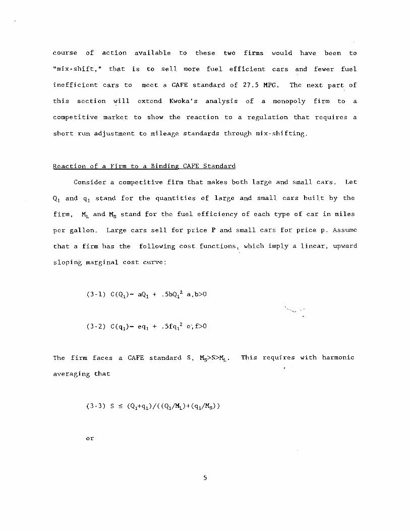
course of action available to these two firms would have been to
"mix-shift, n that is to sell more fuel efficient cars and fewer fuel
inefficient cars to meet a CAFE standard of 27.5 MPG. The next part of
this section will extend Kwoka's analysis of a monopoly firm to a
competitive market to show the reaction to a regulation that requires a
short run adjustment to mileage standards through mix-shifting.
Reaction of a Firm to a Binding CAFE Standard
Consider a competitive firm that makes both large and small cars. Let
Q1 and ql stand for the quantities of large and small cars built by the
firm, ML and Ms stand for the fuel efficiency of each type of car in miles
per gallon. Large cars sell for price P and small cars for price p. Assume
that a firm has the following cost functions, which imply a linear, upward
sloping marginal cost curve:
The firm faces a CAFE standard S, Ms>S>ML •
averaging that
or
5
This requires with harmonic
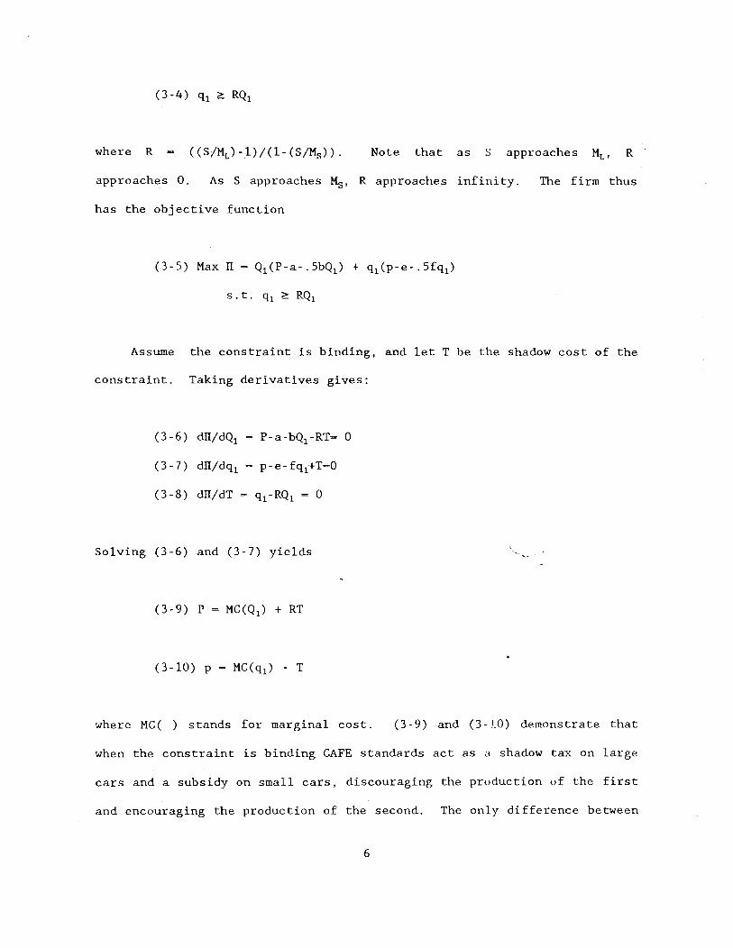
where R «S/ML)-l)/(l-(S/Ms». Note that as S approaches ML, R
approaches O. As S approaches Ms,
has the objective function
R approaches infinity.
(3-5) Max IT = Ql(P-a-.5bQl) + ql(p-e-.5fql)
s.t. ql ~ RQ1
The firm thus
Assume the constraint is binding, and let T be the shadow cost of the
constraint. Taking derivatives gives:
(3-6) dll/dQl
(3-7) dll/dql p-e-fql+T~O
(3-8) dIT/dT = ql-RQl ~ 0
Solving (3-6) and (3-7) yields
(3-9) P = MC(Ql) + RT
(3-10) p ~ MC(Ql) - T
where MC( ) stands for marginal cost.
.~-
(3-9) and (3-10) demonstrate that
when the constraint is binding CAFE standards act as a shadow tax on large
cars and a subsidy on small cars, discouraging the production of the first
and encouraging the production of the second. The only difference between
6
the implicit taxes and subsidies generated by the standard and an explicit
tax/subsidy scheme is that under the CAFE standard the producers get to
keep the tax revenue. This tax revenue, however, must be used to subsidize
the production of small cars.
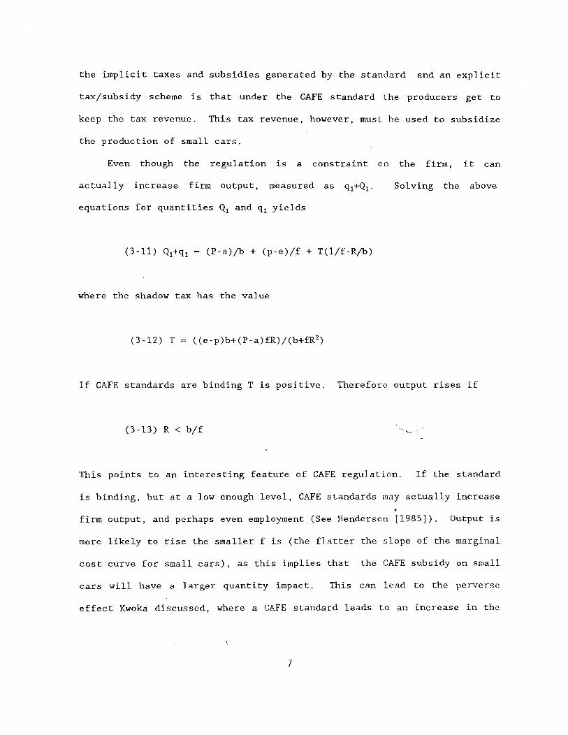
Even though the regulation is a constraint on the firm, it can
actually increase firm output, measured as ql+Ql' Solving the above
equations for quantities Q1 and ql yields
(3-11) Ql+ql - (P-a)jb + (p-e)/f + T(l/f-Rjb)
where the shadow tax has the value
(3-12) T «e-p)b+(P-a)fR)/(b+fR2 )
If CAFE standards are binding T is positive. Therefore output rises if
(3-13) R < b/f ~ ..
This points to an interesting feature of CAFE regulation. If the standard
is binding, but at a low enough level, CAFE standards may actually increase
firm output, and perhaps even employment (See Henderson [1985]). Output is
more likely to rise the smaller f is (the flatter the slope of the marginal
cost curve for small cars), as this implies that the CAFE subsidy on small
cars will have a larger quantity impact. This can lead to the perverse
effect Kwoka discussed, where a CAFE standard leads to an increase in the
7
number of cars on the road, and therefore to an increase in total gasoline
consumption.
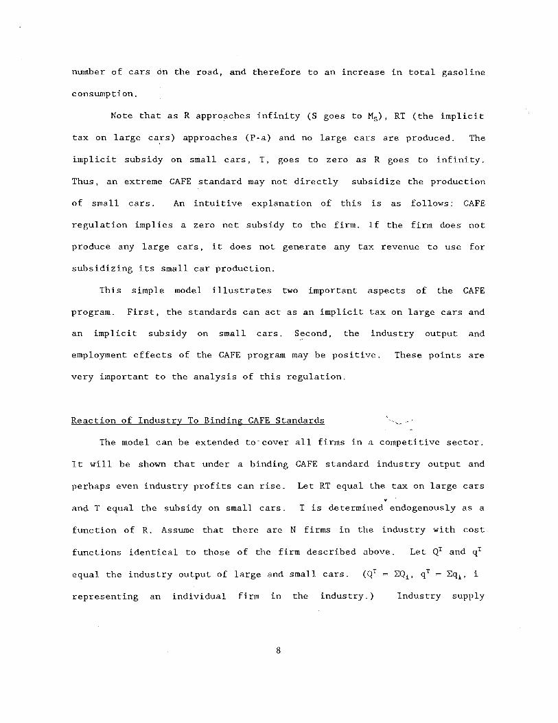
Note that as R approaches infinity (S goes to Ms), RT (the implicit
tax on large ca,rs) approaches (P-a) and no large cars are produced. The
implicit subsidy on small cars, T, goes to zero as R goes to infinity.
Thus, an extreme CAFE standard may not directly subsidize the production
of small cars. An intuitive explanation of this is as follows: CAFE
regulation implies a zero net subsidy to the firm. If the firm does not
produce any large cars, it does not generate any tax revenue to use for
subsidizing its small car production.
This simple model illustrates two important aspects of the CAFE
program. First, the standards can act as an implicit tax on large cars and
an implicit subsidy on small cars. Second, the industry output and
employment effects of the CAFE program may be positive. These points are
very important to the analysis of this regulation.
Reaction of Industry To Binding CAFE Standards
The model can be extended to'cover all firms in a competitive sector.
It will be shown that under a binding CAFE standard industry output and
perhaps even industry profits can rise. Let RT equal the tax on large cars
~
and T equal the subsidy on small cars. T is determined endogenously as a
function of R. Assume that there are N firms in the industry with cost
functions identical to those of the firm described above. Let QT and qT
equal the industry output of large and small cars.
representing an individual firm in the industry.) Industry supply
8

functions are generated by horizontally adding each firm's marginal cost
curve
(3-14) p(QT) - MC(QT) - a+(bQlfN) + RT - a+BQT + RT
(3-15) p(qT) - MC(qT) - e+(fql/N) - T - e+FqT - T
Industry demand curves are
(3-16) p(QT) _ g_hQT
(3-17) p(qT) _ j_kqT
(Cross-price effects are omitted for the sake of simplicity. This omission
does not significantly alter the results of this section.)
firm output and implicit subsidy levels, we have
Solving for
(3-18) T ~ T(R) = (R(g-a)(k+F)-(j-e)(h+B»/(h+B+R2 (k+F»,
(3-19) QT - (g-a-TR)/(h+B) P = g - h(g-a-TR)/(h-t-'B).,
(3-20) qT (j -e+T)/(k+F)' p - j - k(j -e+T)/(k+F).
Total industry output QT + qT is
(3-21) QT+qT - (g-a)/(h+B) + (j-e)/(k+F) + T«l/(k+F»-R/(h+B»)
Similar to the results for one firm shown in (3-13), industry output will
rise as a result of the shadow tax (given R constant) if and only if
9
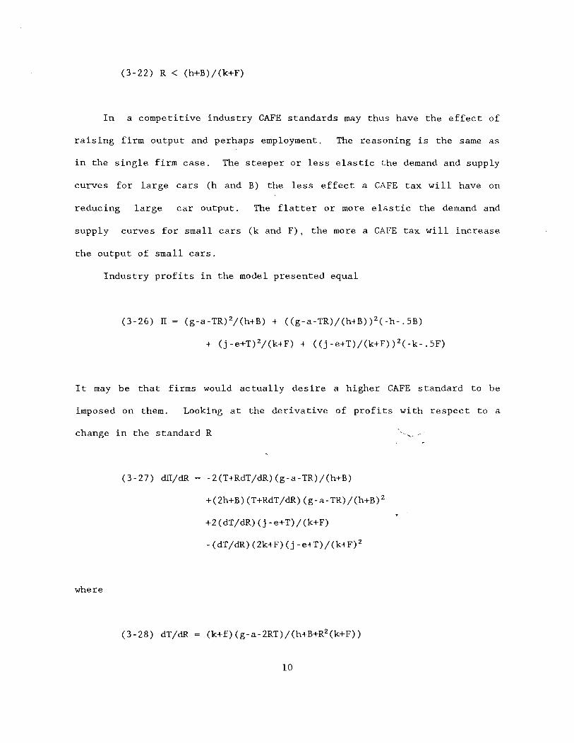
(3-22) R < (h+B)/(k+F)
In a competitive industry CAFE standards may thus have the effect of
raising firm output and perhaps employment. The reasoning is the same as
in the single firm case. The steeper or less elastic the demand and supply
curves for large cars (h and B) the less effect a CAFE tax will have on
reducing large car output. The flatter or more elastic the demand and
supply curves for small cars (k and F), the more a CAFE tax will increase
the output of small cars.
Industry profits in the model presented equal
(3-26) IT = (g-a-TR)2/(h+B) + «g-a-TR)/(h+B»2(-h-.5B)
+ (j-e+T)2/(k+F) + «j-e+T)/(k+F»2(-k-.5F)
It may be that firms would actually desire a higher CAFE standard to be
imposed on them. Looking at the derivative of profits with respect to a
change in the standard R
where
(3-27) dil/dR - -2(T+RdT/dR)(g-a-TR)/(h+B)
+(2h+B) (T+RdT/dR) (g-a-TR)/(h+B)2
+2 (dT/dR) (j-e+T)/(k+F)
-(dT/dR) (2k+F)(j-e+T)/(k+F)2
(3-28) dT/dR = (k+f)(g-a-2RT)/(h+B+R2(k+F»
10
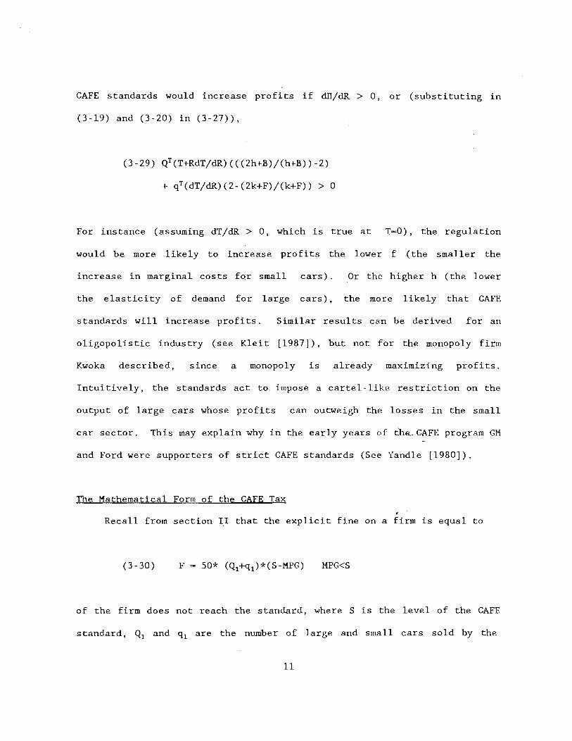
CAFE standards would increase profits if dlI/dR > 0, or (substituting in
(3-19) and (3-20) in (3-27»,
(3-29) QT(T+RdT/dR)«(2h+B)/(h+B»-2)
+ qT(dT/dR) (2-(2k+F)/(k+F» > 0
For instance (assuming dT/dR > 0, which is true at T=O) , the regulation
would be more likely to increase profits the lower f (the smaller the
increase in marginal costs for small cars). Or the higher h (the lower
the elasticity of demand for large cars), the more likely that CAFE
standards will increase profits. Similar results can be derived for an
oligopolistic industry (see Kleit [1987]), but not for the monopoly firm
Kwoka described, since a monopoly is already maximizing profits.
Intuitively, the standards act to impose a cartel-like restriction on the
output of large cars whose profits can outweigh the losses in the small
car sector. This may explain why in the early years of the. CAFE program GM
and Ford were supporters of strict CAFE standards (See Yandle [1980]).
The Mathematical Form of the CAFE Tax . Recall from section II that the explicit fine on a firm is equal to
(3-30) MPG<S
of the firm does not reach the standard, where S is the level of the CAFE
standard, Q1 and ql are the number of large and small cars sold by the
11
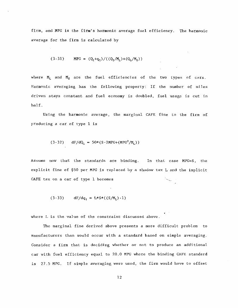
firm, and MPG is the firm's harmonic average fuel efficiency. The harmonic
average for the firm is calculated by
(3-31)
where ML and lis are the fuel efficiencies of the two types of cars.
Harmonic averaging has the following property: If the number of miles
driven stays constant and fuel economy is doubled, fuel usage is cut in
half.
Using the harmonic average, the marginal CAFE fine to the firm of
producing a car of type 1 is
(3-32)
Assume now that the standards are binding. In that case MPG-S, the
explicit fine of $50 per MPG is replaced by a shadow tax L and the implicit
CAFE tax on a car of type 1 becomes
(3-33)
where L is the value of the constraint discussed above.
The marginal fine derived above presents a more difficult problem to
manufacturers than would occur with a standard based on simple averaging.
Consider a firm that is deciding whether or not to produce an additional
car with fuel efficiency equal to 20.0 MPG where the binding CAFE standard
is 27.5 MPG. If simple averaging were used, the firm would have to offset
12
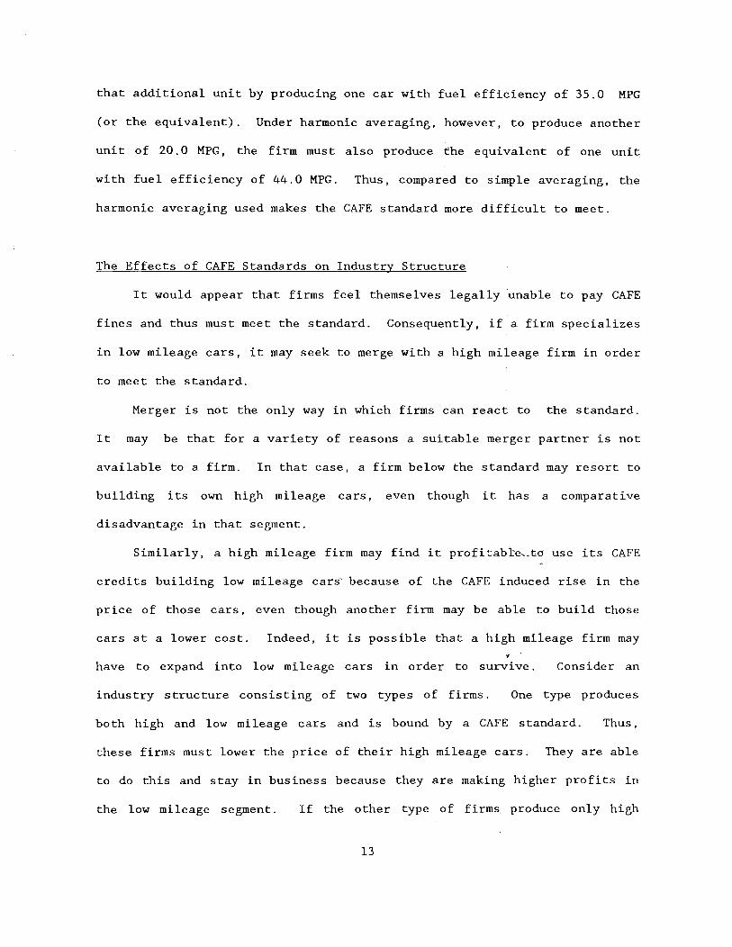
that additional unit by producing one car with fuel efficiency of 35.0 MPG
(or the equivalent). Under harmonic averaging, however, to produce another
unit of 20.0 MPG, the firm must also produce the equivalent of one unit
with fuel efficiency of 44.0 MPG. Thus, compared to simple averaging, the
harmonic averaging used makes the CAFE standard more difficult to meet.
The Effects of CAFE Standards on Industry Structure
It would appear that firms feel themselves legally unable to pay CAFE
fines and thus must meet the standard. Consequently, if a firm specializes
in low mileage cars, it may seek to merge with a high mileage firm in order
to meet the standard.
Merger is not the only way in which firms can react to the standard.
It may be that for a variety of reasons a suitable merger partner is not
available to a firm. In that case, a firm below the standard may resort to
building its own high mileage cars, even though it has a comparative
disadvantage in that segment.
Similarly, a high mileage firm may find it profitable",td use its CAFE
credits building low mileage car~ because of the CAFE induced rise in the
price of those cars, even though another firm may be able to build those
cars at a lower cost. Indeed, it is possible that a high mileage firm may
have to expand into low mileage cars in order to survive. Consider an
industry structure consisting of two types of firms. One type produces
both high and low mileage cars and is bound by a CAFE standard. Thus,
these firms must lower the price of their high mileage cars. They are able
to do this and stay in business because they are making higher profits in
the low mileage segment. If the other type of firms produce only high
13
mileage cars they are at a serious disadvantage. They must sell their
products in a market where their competitors are being subsidized by
lucrative sales of large cars. Given this situation, a high mileage firm
may have no choice but to expand into low mileage cars.
Thus, a binding CAFE standard creates what may best be described as
regulatory economies of scope in the auto industry. No firm can legally be
below the standard and no firm can afford to be above the standard.
Therefore, in a regime of binding CAFE standards it could be expected that
in the long run all firms in the industry will converge towards the CAFE
standard. Thus, all firms will produce both large and small cars.
This result depends on three assumptions. First, standards must be
binding. Second, CAFE credits must not be tradeable across firms. Third,
it must be possible for all firms in one way or another to produce and sell
cars that have mileage above the standard.
IV. SIMULATION OF THE EFFECTS OF CAFE STANDARDS
This section will simulate the effects of various CAFE 'levels on the
automobile market and on energy consumption. The model presented analyzes
whether if enforcing CAFE standards is likely to have the perverse effects
on industry profits, structure and employment, that Section III indicates
are possible. It will also examine if CAFE standards do indeed save
energy. The simulation will make a cost-benefit analysis of the decision
faced by NHTSA for model years 1986 and 1987. If NHTSA had not granted the
relief petitions, firms would have been forced to "mix-shift" in the manner
described above to meet the standards. In the short period available to
14
the firms to change their fleet MPG's, changing the fuel efficiency of
various automobiles would not have been a viable option.
This section is divided into two parts. The first will analyze the
results of a static model of CAFE standards. The effects of various
binding CAFE levels industry profits, employment and structure will be
calculated. The second part will generate any savings in gasoline that
the results of the static model imply. It will chart the course of the
fuel savings from the flow of new automobiles, adjusted for the changes
induced by the imposition of CAFE standards, as well as the change in the
stock of used automobiles due to the change in the price of new cars.
Static Model
The comparative statics model used here is an extension of the 1985
Council of Economic Advisers model used to analyze the effects of import
quotas on the total number of Japanese cars. Model year 1984 is used as
the base period. In the model there are five types of automobiles: 1)
Japanese Basic Small, which includes regular minicompact's-,and subcompacts
such as the Sentra and the Corolla; 2) Japanese Luxury Small, which
includes specialty subcompacts and regular compacts such as the RX7 and the
Stanza; 3) American Basic Small, which includes minicompacts and
subcompacts such as the Cavalier and the Escort; 4) American Luxury Small,
which includes specialty subcompacts and regular compacts such as the
Reliant K and the Mustang; 5) American Large, which includes intermediate
and large cars such as the Cutlass and the LTD. Luxury European cars,
which comprise about 3.5 percent of the market, are excluded from the
model. Other European cars (Volkswagen-Audi and AMC-Renault) are included
15
in the American segments. On-shore Japanese production is included in
the Japanese segments.
Each segment is divided into constrained and unconstrained production.
Constrained are Japanese imports (by the quota) and General Motors and Ford
(by CAFE standards). Unconstrained production includes on-shore Japanese
output, Chrysler, AMC- Renault, and Volkswagen (which under the nuances of
CAFE regulation includes on-shore VW production, off-shore VW production,
and Audi). "Captive" imports (autos built in Japan but sold under American
nameplates) are included in the Japanese segments. The quantities, prices,
and fuel efficiencies for each type of car for model year 1984, are shown
in Table 1. 5
Equilibrium prices and quantities are computed through a series of
five demand and five supply equations. Quantity demanded is determined by
a set of linear demand curves6
(4-1) Q - AP + B
....... '
where Q a the vector of five quantities, P is the price vector, A is a five
by five matrix of slope coefficients, and B is a vector of intercepts.
5 Actual final mileage figures are somewhat above those reported in Table 1. There are two possible reasons for this discrepancy. First, EPA mileage figures are subj ect to revision for CAFE regulatory purposes. Second, Ward's segment data are calculated through registration data for calendar, not model years. Data included in the 1985 yearbook includes some sales for model year 1985 (fourth quarter 1984), which could have reflected as increased consumer demand for large cars.
6 With the imposition of a standard, linear curves generate less deadweight loss than constant elasticity curves.
16
Quantity supplied is determined by a set of linear supply curves
(4-2) Q = C(P-T) + DP + E
where C is a diagonal five by five matrix of sur'ply coefficients for
constrained firms, D a diagonal five by five matrix of supply coefficients
for the unconstrained firms, E a vector of supply curve intercepts, and T
is a vector of implicit taxes, T' = (T1, Tz, T3 , T4 , Ts). Note that T is
only applied to constrained firms. Tl and Tz are the implicit tariffs for
each type of off-shore Japanese car, T1-Tz . T3 , T4 , Ts are the implicit
CAFE taxes applied to each type of American car produced by constrained
firms GM and Ford. 7 The level of these taxes will be generated by the
model.
During the 1980s, Japanese car sales in the United States have been
restricted by import quotas (so-called "voluntary res traint agreements").
The implicit tariff generated by the quota is set at an initial level of
$2400 and is assumed to be equal for each type of Japnnes~,~ar. Given the
elasticity assumptions of this model, a tariff of $2400 is consistent with
Crandall [1984].8 The quota is set at 1.85 million cars. CAFE standards
are assumed to be just non-binding in the initial conditions and equally
7 Assume that under one scenario in the model the implicIt tariff on Japanese cars is $2500 and the implicit CAFE tax is $300 per MPG. Using the formula for calculating implicit CAFE taxes (3 - 33) and the MPG per class in Table 1 yields an implicit tax vector T' (2500, 2500, 300*27.5*«27.5/33.30)-1), 300*27.5*«27.5/26.72)-1), 300*27.5*«27.5/22.30)-1» - (2500, 2500, -1437, 241, 1924).
8 Assuming a supply elasticity of 2, a demand elasticity of 3.5, and an increase in the price of Japanese cars of $872 yields an implicit tariff of $2400. Crandall estimates the price impact of quotas for Japanese cars as being from $800 to $1000.
17
binding on the "Big Two" (General Motors and Ford) if the policy is
enforced. 9 This is likely to yield an underestimate of deadweight loss, as
DWL is a function of the implicit tax squared and Crandall [1986] suggests
that even without relief CAFE standards would be binding on GM and Ford.
If CAFE standards are imposed, they are assumed to be binding, and the
implicit tax per "Big Two" car is calculated according to equation [3-33].
The system of 12 equations (five demand curves, five supply curves, and
two constraints) in 12 unknowns (five quantities, five prices, and two
implicit taxes) is solved and the implicit tariff and the shadow tax per
MPG are iterated until the desired quota and CAFE standard level are
reached.
The point elasticities of demand at the original 1984 equilibrium are
shown in Table 2. The own elasticity of demand for automobiles as a whole
is assumed to be one. (This is consistent with the results reported in
Irvine[1983].) It is assumed here that the demand for small cars is more
elastic than the demand for large cars, though this is questioned by
Langenfeld and Munger [1985]. The cross-elasticities snown are not meant
to be accurate figures, but merely internally consistent. The method for
the derivation of the cross-elasticities is presented in the technical
appendix (which is available from the author).
To this author's knowledge, no study exists of short-run cost curves
in the auto industry. Results of Friedlander et. al. [1983] indicate that
the industry may have constant long-run marginal cost curves. In the short
run, however, it seems likely that marginal costs are increasing. Thus, the
9 Chrysler is assumed not to be bound by CAFE regulations in the simulation. Its supply of credits earned in previous years are more than sufficient to cover any likely shortfall.
18
point elasticity of supply (marginal cost) in the model is set equal to 2,
which assumes that while the industry has a competitive structure, there
are rents to be earned in the sale of automobiles.
Results of Static Model
The most obvious conclusion to be derived from running the static
model is that imposing CAFE standards can create tremendous losses for the
economy. For instance, imposing an increase in fuel economy levels of 1.5
MPG costs the economy about $3.5 billion. This is of the same magnitude
as the losses from import quotas on Japanese cars (See Crandall [1984]).
As for winners and losers, it depends on how tight a CAFE standard is set.
Effects of Firms, Autoworkers. and Consumers
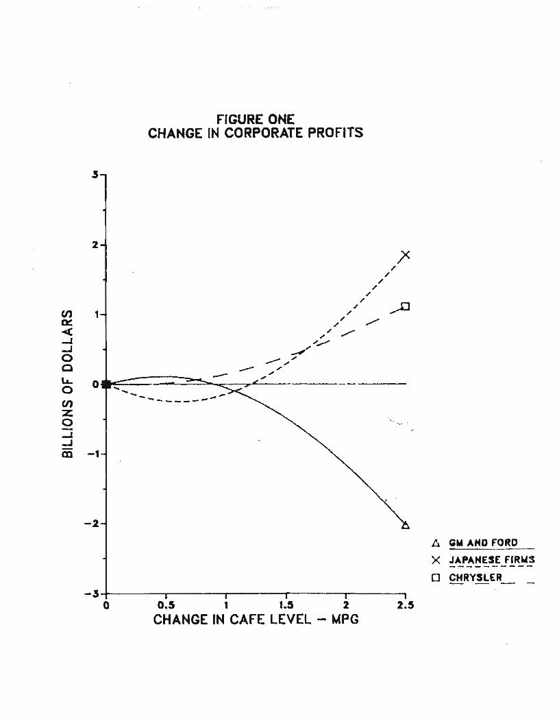
Figure 1 shows the changes in profits for the Big Two companies,
Chrysler, and the Japanese firms. It turns out that it is not all that
unlikely for the constrained firms to have increased profits as a result of
increased fuel economy levels. At CAFE- imposed fuel ec'onomy increases of
below 0.9 MPG profits of GM and Ford rise, reaching a level of $144 million
with an increase of 0.5 MPG. Viewed in this context, Big Two support for
higher CAFE levels in the 1970s is not at all surprising . .-
Unfortunately for the Big Two, profits turn sharply negative after 0.9
MPG. At increases of 1.5 MPG the Big Two suffer losses of almost $500
million, and at 2.5 MPG their estimated regulation induced losses are over
$2 billion. This would seem to explain why GM and Ford were so eager to
gain relief for both model years 1985 and 1986.
19
The impact of CAFE regulations on Chrysler's profits are quite
different. Chrysler loses a little money (at most $10 million) at low CAFE
increase levels as increased Big Two small car sales lower the price
Chrys ler can gain for its small cars. However, at higher CAFE levels
Chrysler's profits are sharply positive as Chrysler increases its sale of
large cars while GM and Ford are severely constrained in that segment. A
CAFE increase of 1.5 MPG raises Chrysler profits by $386 million, while an
increase in CAFE levels of 2.5 MPG reaps a windfall of over $1 billion for
the nation's number three automaker. This may explain why Chrysler is such
a vocal supporter of CAFE standards.
Japanese firms did not produce any large cars and hence would seem to
be more vulnerable in the short run to CAFE increases than Chrysler. With
a CAFE increase of up to 1.1 MPG the Japanese lose money as GM and Ford
lower small car prices. However, as CAFE standards rise above that level,
more and more would-be large car buyers switch into Japanese luxury small
cars, resulting in increasing Japanese profits. With a CAFE increase of
1.5 MPG the Japanese gain $313 million in profits, and at'2~5MPG they make
about $1.8 billion. Given the inherent range of error in a simulation like
this one, it is not at all clear whether Japanese firms stand to gain from
an increase in CAFE levels of 1.5 MPG.
~
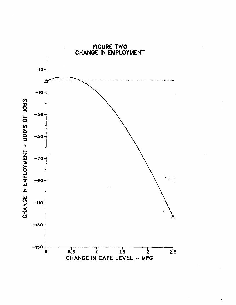
Figure 2 illustrates the effects of higher CAFE levels on automobile
industry employment. Potential gains for autoworkers through CAFE
regulation appear to be quite small. At most, imposing a higher CAFE level
results in an increase of only about 4000 jobs. However, as the CAFE
levels increases, the effect on autoworkers turns sharply negative. With a
CAFE increase of 1.5 MPG 37,900 jobs are lost, and imposing an increase of
20
2.5 MPG results in the loss of 121,900 jobs. Thus, while it is possible
CAFE standards can serve as a means of domestic content legislation to
protect industry jobs, they are more likely to reduce auto employment.
Figure 3 illustrates that consumers are the big losers when higher
CAFE standards are imposed. An increase of 1.5 MPG leads to consumer
losses of almost $3.4 billion, while an increase of 2.5 MPG costs consumers
a staggering $8.8 billion. Oddly enough, at very low levels of CAFE
increases, consumers, and the nation as a whole, actually benefit from the
higher standards. What is occurring here is that the extraction of quota
rents from Japanese firms outweighs the deadweight loss resulting from
implicit CAFE subsidies and taxes.
Increasing Big Two CAFE levels by any significant amount generates
large implicit taxes. Increasing CAFE by 0.5 MPG induces a shadow tax of
$241 per MPG on Big Two cars. A CAFE increase of 1.S MPG results in an
implicit fuel efficiency tax of $646, while a shadow tax of $894 per MPG is
required to increase Big Two CAFE levels by 2.5 MPG.
Not surprisingly, the fuel efficiency levels of non'~Qnstrained firms
decrease as the CAFE levels of the Big Two increase. Non-constrained CAFE
levels decline from 30.17 MPG to 29.43 MPG when the Big Two are forced to
increase their CAFE levels by 2.5 MPG. The non-cons trained firms expand
" their share in larger cars and decrease their presence in the small car
market as higher CAFE levels are imposed. This can be taken as at least
partial evidence that imposing CAFE standards creates economies of scope in
the auto industry.
21
Gasoline Consumption Model
To measure the gasoline savings from CAFE standards, it is necessary
to trace the consUmption of new cars sold under the standards for their
entire lifespan and to compare that to the consumption that would take
place without the imposition of CAFE standards. It is also necessary to
take account of the "scrappage effect," the change in the stock of used
cars that results from a change in the price of new cars. Several studies,
such as Gruenspecht [1982] have found that scrappage rates of used cars are
significantly affected by new car prices.
The average miles driven and the scrappage rates for automobiles for
fifteen years after they are sold, obtained from surveys of the Department
of Transportation, are used in the model. The scrappage rates are adjusted
for new car prices changes using the average of Gruenspecht' s results.
Gruenspecht showed that if the price of new cars is raised (lowered), it
causes a significant decrease (increase) in the scrappage rates of used
cars. This effect was so large, in fact, that it was shown that imposition
of more stringent pollution controls would actually cB:us.e' pollution to
increase. It is assumed that Gruenspecht's results hold for each of the
three classes of automobiles (Basic Small, Luxury Small, and Large). For
purposes of the consumption model Japanese cars are combined with their
corresponding American segments.
Much of the fleet changes analyzed above from large car buyers
switching into new cars due to the change in relative prices. Smaller
cars, however, are more fuel efficient, which lowers the marginal cost of
driving, which will encourage more driving. Blair et. al.'s [1984]
estimate of this effect will be used to adjust the miles driven for the new
22
cars coming onto the road. The values of MPG for the three classes can be
determined from the information used in the static model. The entire
fleet fuel efficiency for 1973 is known to be about 14.2 MPG. The model
assumes that the ratio of fuel efficiencies between classes is the same
for each year. With this assumption, knowledge of the fraction of cars
in each class for 1973 and the entire fleet fuel efficiency for 1973, the
fuel efficiency for each class of new car in 1973 can be calculated. It is
also assumed that fuel efficiency grew exponentially for each class of car
between 1973 and 1984. MPG's are then calculated accordingly. Fuel
efficiency for cars made before 1973 is assumed to be equal to 1973 levels
and fuel efficiencies after 1984 are assumed to be equal to 1984 levels.
Results of Consumption Model
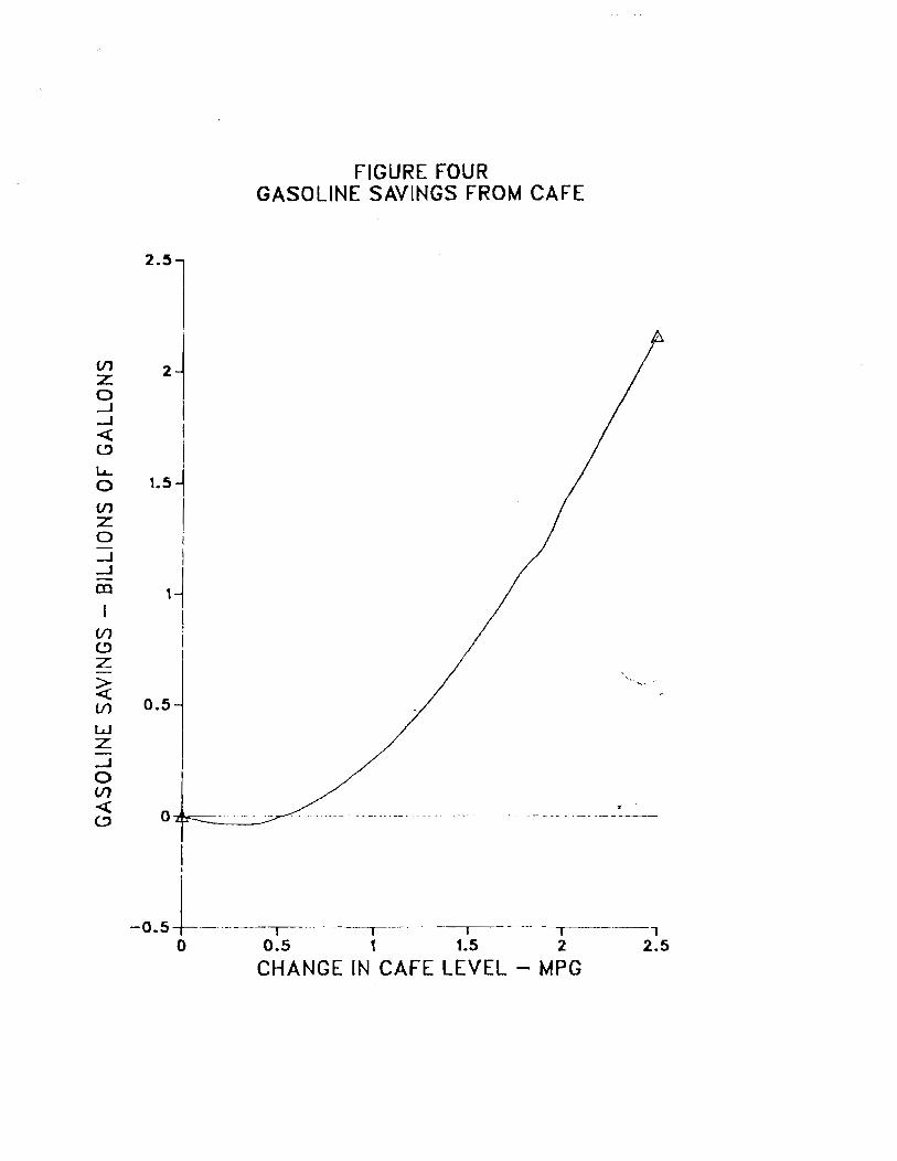
The gasoline consumption results are summarized in Figure 4. The
simulation was run with the CAFE increase of 1.5 MPG in force for one year
and with the additional scrappage and substitution effects described above
for various CAFE levels. A discount rate of 4 percent is',,~~ed.
As noted before, Kwoka hypothesized that CAFE standards could increase
gasoline consumption by placing more cars on the road. Gruenspecht reached
a similar conclusion when he showed that pollution standards could actually
increase pollution levels by raising the price of n~w cars and hence
decreasing the scrappage rates of old cars. Figure 4 shows that CAFE
standards can indeed have such a perverse effect. CAFE level increases of
up to 0.5 MPG do lead to small increases in gasoline consumption (no more
than 43 million gallons out of an annual automobile consumption of about 60
billion) . As CAFE standards grow tighter, fuel savings turn positive,
23
reaching 712 million gallons at 1.5 MPG and 2.105 billion gallons with a
CAFE increase of 2.5 MFG.
While CAFE policy can save gasoline, it does so at a prohibitive cost
to the economy. The average cost per gallon saved with a CAFE increase
of 1.5 MFG is $4.87, which declines slightly to $4.61 with a CAFE increase
of 2.5 MFG.
I t is not appropriate to compare the CAFE- imposed cos t of saving
gasoline with the cost of the gasoline being saved. If gasoline costs $1
per gallon and consumers give up 1 gallon of gasoline, consumers lose, at
the margin, $1 worth of consumption. The loss per gallon noted here is in
addition to this even tradeoff. (See Stucker et. a1. [1980] at 61.) The
true benefit from this policy is the reduction of the externality
associated with gasoline consumption. This also implies that it is
appropriate to discount future savings of gasoline in any cost-benefit
analysis.
Sensitivity Analysis
Given the need to make a large number of assumptions when establishing
this model, it would be informative to see how the robust the conclusions
of this paper are. The most important assumptions of the model are the
relative elasticities of demand (whether demand for sma{l cars is more or
less elastic than the demand for small cars) and the elasticity of supply.
Table 3 shows the results of the model under various supply and demand
elasticity conditions with an increase in CAFE of 1.5 MFG. Supply
elasticities are set at 1. 0, 2.0, and 4.0. A demand elasticity of "same"
refer to the same demand elasticity being used as in the base case.
24
"Alternative" refers to alternative demand elasticities where the own
elasticity of demand for small cars is reduced from 4.00 to 2.50 and the
own elasticity of demand for large cars is increased from 2.50 to 4.00. New
cross-elasticities are then computed using the different assumptions
according to the method described in the technical appendix of this paper.
In five of the six scenarios examined GM and Ford lose a substantial
amount of money, ranging from $234 million to $2.693 billion. Only when the
supply elasticity is 4.0 (which given the circumstances of the industry
would seem extremely high) and the basic scenario is used do they make
money, and then only a bare $64 million.
The results for Chrysler are even more consistent. Chrysler makes
money in every scenario examined, with profits ranging from $311 to $526
million. Thus, it would seem almost certain that enforcement of the higher
standards results in a major windfall for Chrysler.
Japanese firms make money in five of the six scenarios, with profits
ranging from $286 million to $1.903 billion. The most crucial factor for
the Japanese is the elasticity of demand for large cars .',J~~ the large car
elasticity is high, then many would be large car customers respond to
higher prices by looking for alternatives. Japanese luxury small car prices
rise in response to this additional demand, with resulting profits to
Japanese firms.
The effect on consumers is always negative, with losses ranging from
$2.347 billion to $4.646 billion. Auto industry employment declines as
well, with from 25,600 to 59,00 workers being put out of work. From 532
million to 1.084 billion gallons of gasoline are saved, but at an
exorbitant loss to the economy. Costs per gallon range from $3.71 to $6.29.
25
Thus, under a wide range of assumptions imposition of the higher CAFE
standard saves gasoline at a large cost to consumers while benefitting
Chrysler and Japanese firms. GM and Ford, would appear to lose millions and
perhaps billions of dollars from higher standards while job losses in the
auto industry measure in the tens of thousands.
V. CONCLUSION
While CAFE standards were originally designed to decrease consumption
of gasoline in this country, they can have other effects that perhaps were
not considered by the authors of the legislation. By placing a check on
competition in large cars, CAFE regulation can serve to increase the
profits of constrained firms. CAFE standards can also increase domestic
employment in the auto industry and actually increase consumption of
gasoline. The simulation model presented in this paper shows that these
perverse effects can occur, but with varying likelihood. Auto employment
can increase slightly when CAFE standards are imposed, but is more likely
to decline as the standard level increase.
Results for gasoline consumption are similar, as Kwoka's hypothesis is
borne out only at only at CAFE imposed fuel economy increases of less than
0.6 MPG. What does come out of the simulations is that unconstrained firms,
~
if they can adapt to the changed marketplace, have the opportunity to make
a good deal of money as a result of CAFE standards. The profit
possibilities in the large car market can outweigh the losses in the small
car segment. Thus, CAFE regulation encourages and perhaps even forces all
firms to produce each type of automobile, creating regulatory economies of
scope in the industry.
26
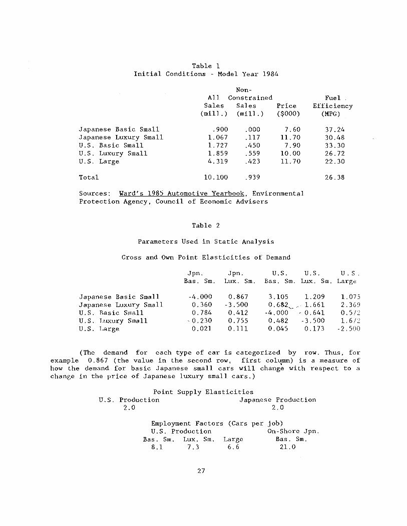
Table 1 Initial Conditions - Model Year 1984
All Sales
(mill. )
NonConstrained
Sales (mill. )
Price ($000)
Fuel Efficiency
(MPG)
Japanese Basic Small .900 .000 7.60 Japanese Luxury Small 1.067 .117 11. 70 U.S. Basic Small 1. 727 .450 7.90 U.S. Luxury Small 1. 859 .559 10.00 u.S. Large 4.319 .423 11.70
Total 10.100 .939
Sources: Ward's 1985 Automotive Yearbook, Environmental Protection Agency, Council of Economic Advisers
Table 2
Parameters Used in Static Analysis
Cross and Own Point Elasticities of Demand
Jpn. Jpn. U.S. U.S.
37.24 30.48 33.30 26.72 22.30
26.38
u.s. Bas. Sm. Lux. Sm. Bas. Sm. Lux. Sm. Large
Japanese Basic Small -4.000 0.867 3.105 1.209 1.075 Japanese Luxury Small 0.360 -3.500 0.68.2 '-- .- 1. 661 2.369 u.S. Basic Small 0.784 0.412 -4.000 ~ 0.641 0.572 u.S. Luxury Small ,0.230 0.755 0.482 -3.500 l.672 u.S. Large 0.021 0.111 0.045 0.173 -2.500
(The demand for each type of car is categorized by row. Thus, for example 0.867 (the value in the second row, first column) is a measure of how the demand for basic Japanese small cars will chang~ with respect to a change in the price of Japanese luxury small cars.)
Point Supply Elasticities u.S. Production
2.0 Japanese Production
2.0
Employment Factors (Cars U.S. Production
Bas. Sm. Lux. Sm. Large 8.1 7.3 6.6
27
per job) On-Shore Jpn.
Bas. Sm. 21.0
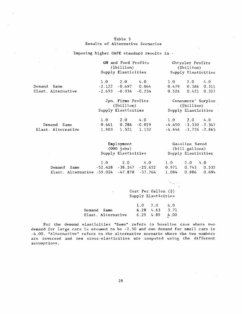
Table 3 Results of Alternative Scenarios
Imposing higher CAFE standard results in -
Demand Same Elast. Alternative
Demand Same Elast. Alternative
GM and Ford Profits ($billion)
Supply Elasticities
1.0 -2.122 -2.693
2.0 -0.497 -0.934
4.0 0.064
-0.234
Jpn. Firms Profits ($billion)
Supply Elasticities
1.0 0.661 1. 903
2.0 0.286 1.521
Employment
4.0 -0.019 1.132
(000 jobs) Supply Elasticities
1.0 Demand Same -52.428 Elast. Alternative -59.024
2.0 -38.247 -47.878
4.0 -25.652 -37.764
Chrysler Profits ($billion)
Supply Elasticities
1.0 0.479 0.526
2.0 0.386 0.421
4.0 0.311 0.327
Consumers' Surplus ($billion)
Supply Elasticities
1.0 -4.450 -4.646
2.0 4.0 -3.330 -2.347 -3.726 -2.865
Gasoline Saved (bill. gallons)
Supply Elasticities
1.0 0.971 1.084
2.0 0.743 0.886
4.0 0.532 0.694
Cost Per Gallon ($) Supply Elasticities
Demand Same Elast. Alternative
1.0 6.28 6.29
2.0 4.63 4.89
4.0 3.71 4 . .00 ~
For the demand elasticities "Same" refers to baseline case where own demand for large cars is assumed to be -2.50 and own demand for small cars is -4.00. "Alternative" refers to the alternative scenario where the two numbers are reversed and new cross-elasticities are computed using the different assumptions.
28
en IX ~ ...J ...J o C La.. o en z o -...J ...J -
2
1
o ....
ell -1
-2
FIGURE ONE CHANGE IN CORPORATE PROFITS
-," --",,"" -- -- ",,"" ""
'........... .,.. ... ..... ------~
" "
" " " ,/" ..-...0
,," / ,," /
",......
-3-+-------.,...----------------.-------. o 0.5 1 1.5 2 2.5
CHANGE IN CAFE LEVEL - MPG
A gilt AHD FORO
X JAPANESE FlRWS ----------o CHRYSLER_ _
(J) CD 0 -, I.&.. 0 (J) -0 0 0
I t-Z ..... ::E >-0 ...J 0.. ~ LaJ
Z
LaJ
" Z < :c 0
10
-to
-30
-50
-70
-10
-ltO
-130
FIGURE TWO CHANGE IN EMPLOYMENT
-150~------------------~~------------o 0.5 1 1.5 2 2.5
CHANGE IN CAFE LEVEL - MPG
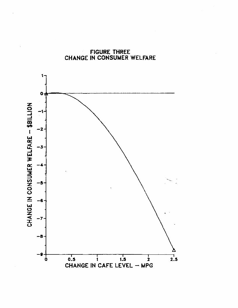
FIGURE THREE CHANGE IN CONSUMER WELFARE
1
0
z 0
-1 -.... ...I -CD .... ( -2
LaJ 0::::
~ -3 ...J LaJ ~ 0:: -4 LaJ :l: ::::::. (I) -5
~ ..
Z 0 (.)
Z -6 LaJ (!)
Z < -7 ::I: (.)
-8
-I~----~------~-------------------o 0.5 1 1.5 2 2.5 CHANGE IN CAFE LEVEL - MPG
V')
C> Z
~ V')
w Z -.J o (f)
~ C>
0.5
o
I I
FIGURE FOUR GASOLINE SAVINGS FROM CAFE
• - ...... ----.. _ .. -------- .... ------_.- ._-----_._------
-0.51-----,-------- I I --'1"--- ------. o 0.5 t 1.5 2 2.5
CHANGE IN CAFE LEVEL - MPG
REFERENCES
Bamberger, Robert Economy Standards," 21, 1984
L., "Prospects Congressional
of Non-Compliance with Automobile Fuel Research Service, Washington, D.C. December
Berkovic, James, "New Car Sales and Used Car Stocks," Rand Journal of Economics. Summer 1985, pages 195-214
Blair, Roger D., David L. Kaserman, and Richard C. Tepel, "The Impact of Improved Mileage on Gasoline Consumption," Economic Inquiry, April, 1984, pp.209-217
Bohi, Douglass R., Analyzing Demand Behavior: A Study of Energy Elasticities Johns Hopkins, Baltimore, 1981
Bryan, Michael F., and Owen F. Humpage, "Voluntary Export Restraints: The Cost of Building Walls" Economic Review (Federal Reserve Bank of Cleveland) Summer 1984, pages 17-37.
Department of Commerce (United States), "Comments on Issues Raised in Petitions by General Motors Corporation and Ford Motor Company," Washington, D.C., April 30, 1985
Council of Economic Advisers, "Impact of the Japanese Automobile Voluntary Restraint Agreemcnt," Mimeo, February, 1985
Crandall, Robert W., "Import Quotas and the Automobile Industry, The Brookings Review, Summer 1984, pages 8-16
Crandall, Robert, "Why Should We Regulate Fuel Economy At All?" The Brookings Review Vol. 3, No.3, Spring 1985, pp.3-8
Crandall, Robert Lave, Regulating 1986
F., Howard K. Gruenspecht, Theodore E. the Automobile, The Brookings Institution,
Keeler, Lester B. Washington, D.C.,
Friedlander, A.F., C. Winston, and K. Wang, "Costs, Technology, and Productivity in the U.S. Automobile Industry," Bell Journal of Economics, Winter, 1982, pp.I-20.
Gruenspecht, Howard K., "Differentiated Regula lion: A Theory Applications to Automobile Emissions Controls" Yale University Dissertation, 1982
with Ph.D.
Henderson, David R., "The Economics of Fuel Economy Standards", Regulation January/February 1985, pp. 45-48
Hess, Alan C. "A Comparison of Automobile Demand Equations", Econometrica 45(3):680-701, April, 1977
29
Irvine, F. Owen Jr., "Demand Equations for Individual New Car Models", Southern Economic Journal Jan. 1983 pp. 764-782
Kalt, Joseph P. The Economics and Politics of Oil Price Regulation MIT Press, Cambridge, MA 1981
Kleit, Andrew N., "The Economics of Automobile Fuel Economy Standards," Yale University Ph.D. dissertation, 1987
Knoll, Michael S., "The Economics of the Corporate Average Fuel Economy Standards and Their Effect on Automobile Prices", mimeo, International Trade Commission, 1986
Kwoka, John E. Jr., "The Limits of Market Oriented Regulatory Techniques: The Case of Automotive Fuel Economy", The Ouarterly Journal of Economics, November 1983, pp. 695-704
Langenfeld, James A., and Michael C. Munger, "The I mpact of Federal Automobile Emissions," Mimeo, Federal Trade Commission (J une, 1985)
Parks, Richard W., "Determinants of Scrappage Rates for Postwar Vintage Automobiles", Econometrica 45(5):1099-1115, 1977
Rogers, Robert P., "The Short-Run Impact of Changes in the Corporate Average Fuel Economy Standards," mimeo, Federal Trade Commission, May 12, 1986
Stucker, J.P., B.K. Burright, and W.E. Mooz, "Evaluating Fuel Economy Mandates", A Rand Note N-I005, February, 1980
Sweeney, James L., "New Car Efficiency Standards and the Demand for Gasoline", Advances in the Economics of Energy and Resources Vol. 1, pp. 105-133, 1979
White, Lawrence J., The Automobile Industry Since 1945 University Press, Cambridge MA, 1971
Yandle, Bruce, "Fuel Efficiency by Government Mandate: A Cost-Benefit Analysis", Policy Analysis Volume 6, Number 3 Summer InO, pages 291-304.
30
Recommended

![Advances in Automobile Hamzehlouia et al., Engineeringaizadian/index_files/Papers/J-6.pdf · Advances in Automobile Engineering. Hamzehlouia et al., ... [9,10] report 79% fuel economy](https://img.pdfslide.us/doc/110x75/5ab347497f8b9aea528e285f/advances-in-automobile-hamzehlouia-et-al-aizadianindexfilespapersj-6pdfadvances.jpg)