No. 14-10
The Forecasting Power of Consumer Attitudes for Consumer Spending
Michelle L. Barnes and Giovanni P. Olivei
Abstract: We assess the ability of the Reuters/Michigan Surveys of Consumers to predict future changes in consumer expenditures. The information in the Surveys is summarized by means of principal components of consumer attitudes with respect to income and wealth, interest rates, and prices. These summary measures contain information that goes beyond the information captured by the Index of Consumer Sentiment from the same Surveys. The summary measures have forecasting power for aggregate consumption behavior, even when controlling for current and future economic fundamentals. These measures also help to explain a nontrivial portion of consumption and other real activity forecast errors from the Survey of Professional Forecasters and the Federal Reserve Board’s Greenbook. This finding is consistent with the ability of these summary measures to predict consumption even when conditioning on a broader set of funda-mentals and on forecasters’ judgmental assessments of developments that are not easily quantifiable.
JEL Classifications: E21, E27, E52, E66
Michelle L. Barnes is a senior economist and policy advisor in the research department at the Federal Reserve Bank of Boston. Her e-mail address is [email protected]. Giovanni P. Olivei is a vice president and head of the macro-international group in the research department at the Federal Reserve Bank of Boston. His e-mail address is [email protected]. The authors thank Ye Ji Kee for excellent research assistance. This paper presents preliminary analysis and results intended to stimulate discussion and critical comment. The views expressed herein are those of the authors and do not indicate concurrence by the Federal Reserve Bank of Boston, or by the principals of the Board of Governors, or the Federal Reserve System. This paper, which may be revised, is available on the web site of the Federal Reserve Bank of Boston at http://www.bostonfed.org/economic/ppdp/index.htm. This version: October 30, 2014

1. Introduction
The Reuters/Michigan Index of Consumer Sentiment’s ability to explain consumer
expenditures has been extensively studied in the literature, and a consensus has emerged that
the role of consumer sentiment in consumption is typically small from an economic standpoint,
even if often statistically significant. This finding is especially true when controlling for
economic fundamentals: in this case, the independent information from sentiment is limited
and arises at least in part from sentiment’s ability to forecast subsequent developments in
income and, more generally, in aggregate demand.1
Despite the prevalence of studies pertaining to consumer sentiment, little attention has been
devoted to assessing the role that more broadly defined consumer attitudes play in
consumption behavior. The widely studied Index of Consumer Sentiment, a representative
measure of survey-based assessments of sentiment, is constructed from the answers to five
survey questions.2 These questions, however, are part of a more comprehensive survey of
consumers’ attitudes and expectations, the Reuters/Michigan Surveys of Consumers. In this
paper, we exploit this broader set of questions to investigate which aspects of consumer
attitudes matter for consumption behavior. In doing so, one challenge is devising a way to
summarize the information contained in the questions from the Surveys in a manner that is
economically meaningful. We propose a limited set of summary measures of various aspects of
the economic environment covered by the Surveys. These measures are constructed from
1 See Carroll, Fuhrer, and Wilcox (1994) and Fuhrer (1993). For a survey of the literature on the role of consumer sentiment in consumer spending dynamics, see Ludvigson (2004).
2 The five equally weighted questions that compose the sentiment index are the following:
(1) "We are interested in how people are getting along financially these days. Would you say that you (and your family living there) are better off or worse off financially than you were a year ago?"
(2) "Now looking ahead—do you think that a year from now you (and your family living there) will be better off financially, or worse off, or just about the same as now?"
(3) "Now turning to business conditions in the country as a whole—do you think that during the next twelve months we'll have good times financially, or bad times, or what?"
(4) "Looking ahead, which would you say is more likely—that in the country as a whole we'll have continuous good times during the next five years or so, or that we will have periods of widespread unemployment or depression, or what?"
(5) "About the big things people buy for their homes—such as furniture, a refrigerator, stove, television, and things like that. Generally speaking, do you think now is a good or bad time for people to buy major household items?"
1
subsets of the questions from the Reuters/Michigan Surveys of Consumers, with each subset
corresponding to a broad economic determinant of consumption—income, wealth, prices, and
interest rates.
We find that a noticeable portion of the information in the broader Surveys is not being
captured by the widely studied headline Index of Consumer Sentiment (or, interchangeably,
“consumer sentiment”), which is constructed from the five questions detailed in footnote 2
above. More importantly, the information embedded in our summary measures has
explanatory power for consumption behavior beyond that of the consumer sentiment index
itself. This information in our broader summary measures pertains to consumer attitudes
toward interest rates, credit availability, and prices. In particular, the informational content
from responses regarding the interest rate appears to be robust across various specifications and
sample periods. While the information pertaining to consumer attitudes toward income and
wealth does have explanatory power for consumption, this portion of the broader survey
information is well conveyed by the summary measure of consumer sentiment.
The power of the Surveys’ summary measures for forecasting consumption is robust to the
inclusion of fundamentals. As with previous results in the literature concerning consumer
sentiment, the improvement in forecasting power is relatively limited but, compared to the
inclusion of sentiment only, is significant from a statistical standpoint and is economically
relevant at times. The summary measures’ ability to forecast future consumption growth
continues to hold when, instead of controlling for lagged fundamentals, we control for
fundamentals that are contemporaneous with consumption growth. This result is shown in the
context of an augmented Campbell and Mankiw (1990) framework, and expands on the results
in Carroll, Fuhrer, and Wilcox (1994).
The summary measures’ ability to forecast future consumption growth even in the presence
of fundamentals, whether lagged or contemporaneous to consumption growth, is not easily
explained. The potential reasons that involve the omission of relevant determinants of
consumption, such as uncertainty, are not necessarily consistent with our empirical findings. In
some cases, our measured fundamentals are only a proxy for the true fundamental. For
example, this issue arises for the interest rate measure we are controlling for, which is not
2

perfectly correlated with the actual cost of credit faced by consumers. In sum, we cannot rule
out that a larger and more precisely measured set of fundamentals may overturn some of our
findings.
We address this issue to some extent, however, by showing that the summary measures
taken from the broader Surveys have significant explanatory power for real side forecast errors
that inform the Survey of Professional Forecasters and the Federal Reserve Board’s Greenbook.3
Presumably, these forecasts are conditioned on a broader set of fundamentals than those we
consider in our forecasting exercises. Furthermore, these forecasts contain a judgmental
component that in principle could capture animal spirits or other features of the economic
environment. These features are hard to measure and could be correlated with the portion of
the survey’s summary measures that is orthogonal to fundamentals. Still, these measures have a
sizable explanatory power for the forecast errors. This finding is true not just for the
consumption growth forecast errors, but also for broader activity measures such as real GDP
growth and the unemployment rate.
Our paper is related to previous work by Slacalek (2006), who used the same principal
components approach we employ here to summarize the questions in the Reuters/Michigan
Surveys of Consumers. To our knowledge, this is the only other paper assessing the Surveys’
information content for consumption. Our approach differs from Slacalek’s work in that we
consider a more detailed, and hence larger, set of questions, and we form our principal
components in such a way as to link them to fundamentals. Moreover, to better assess the
forecasting power of the information contained in the Surveys, the principal components are
constructed in real time. The scope of our exercise is also different because we assess the
Surveys’ ability to predict consumption in a broader context that controls for fundamentals in a
variety of ways.
While in principle there are different approaches to summarizing information from a large
dataset, our approach has the advantage of relating the Surveys’ information to important
economic determinants of consumption. This allows us to ascertain the relationship between the
3 The Greenbook forecast of the U.S. economy is produced by the research staff of the Federal Reserve Board before each FOMC meeting to support the FOMC members in their policy deliberations.
3
survey data and consumption dynamics in a more transparent way than by resorting to
summary measures of the survey information that do not have an immediate correspondence to
an economic fundamental. For example, one can speak directly to consumers’ attitudes or
expectations about wealth and income or interest rates in isolation, as opposed to using some
indices that may confound the influence of a number of different drivers of consumption.
Moreover, when controlling for fundamentals, having summary measures from the Surveys
that can be linked, albeit broadly, to these fundamentals can help further elucidate what
information in the Surveys might play an independent role in explaining consumption
dynamics.
The rest of this paper proceeds as follows. In Section 2, we briefly describe the
Reuters/Michigan Surveys of Consumers, the construction of the real-time summary measures
from the Surveys’, and the summary measures’ relationship with the Index of Consumer
Sentiment and commonly measured fundamentals. Section 3 analyzes the forecasting power of
the real-time survey measures for consumption, considered both in isolation and when
controlling for fundamentals. Section 4 uses a Campbell-Mankiw type of framework to show
that even if the summary measures based on the Surveys’ have predictive power for future
fundamentals, these measures still play an independent role in consumption dynamics. In
Section 5 we show that these real-time survey measures have substantial explanatory power for
both Survey of Professional Forecasters and Greenbook forecast errors. Section 6 provides
concluding remarks.
2. The Reuters/Michigan Surveys of Consumers
This section describes how we summarize the information from a broad range of questions in
the Reuters/Michigan Surveys of Consumers (in what follows this is referred to by the abridged
“Surveys of Consumers,” or “Surveys,” as used above), and how this information relates to
commonly measured fundamentals. Based on a representative sample of households in the 48
contiguous United States, the Surveys’ questions range from inquiring about an individual
household’s own current and expected financial situation to its assessment of the broader
4
economic environment in terms of unemployment, inflation, the buying conditions for a variety
of products, and other topics. We select 42 questions from the Surveys of Consumers that
pertain to income, wealth, prices, and interest rates. For these variables, the questions may refer
to current or expected developments and to developments that are household-specific or
economy-wide. The Appendix has a list of the 42 questions we draw from the Surveys.
The selected questions can be viewed as complementing and adding detail to the five survey
questions used to construct the Reuters/Michigan Index of Consumer Sentiment. For example,
one of the questions included in the consumer sentiment index is “Do you think now is a good
or bad time for people to buy major household items?” For this question, the Surveys also ask
why participants have a particular perception about buying major household items. The reasons
pertain to different aspects of the current and expected economic environment, such as income
and prosperity, interest rates and credit availability, and prices. Rather than just considering the
answer to the higher-level summary question, our analysis includes the reasons that households
provide to justify their answers to the higher-level question.
A large portion of the Surveys, however, features questions that are not directly or indirectly
related to the questions upon which the consumer sentiment index is formed. Several of these
questions, such as whether the respondent thinks it is a good time to buy a home or not, share
the same multiple-level structure we have just illustrated. For this type of multi-layered
question, we thus follow a similar procedure. Other questions, such as a household’s
expectations about unemployment during the coming 12 months, do not have sub-questions
delving deeper into their reasoning, and we include these directly to the extent that they can be
attributed to a particular feature of the economic environment.
The questions we select from the Surveys of Consumers typically elicit a qualitative
response. Consequently, these responses can be used as the basis for constructing a diffusion
measure of how favorably respondents view a certain economic development. For example,
with respect to the question about buying conditions for major household items, the selection of
“Good Time to Buy: Interest Rates are Low” to the sub-question about why this is a good time
to buy a major household item indicates the percentage of respondents who chose this
particular answer from several potential selections. For this type of question, the Surveys of
5
Consumers also includes a mirroring question about why this is a bad time to buy a major
household item, including the possible response, “Bad Time to Buy: Interest Rates are High.”
Thus, from the responses, it is possible to provide a diffusion index for how important low
interest rates are in the respondents’ assessment of buying conditions for major household
items, which is constructed by subtracting the percentage of those who chose the “Good Time to
Buy: Interest Rates Are Low” response to the first question from the percentage of respondents
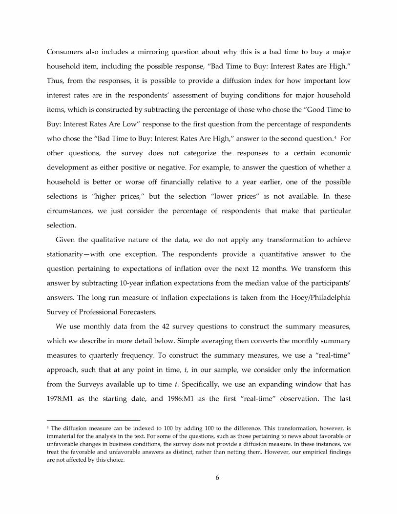
who chose the “Bad Time to Buy: Interest Rates Are High,” answer to the second question.4 For
other questions, the survey does not categorize the responses to a certain economic
development as either positive or negative. For example, to answer the question of whether a
household is better or worse off financially relative to a year earlier, one of the possible
selections is “higher prices,” but the selection “lower prices” is not available. In these
circumstances, we just consider the percentage of respondents that make that particular
selection.
Given the qualitative nature of the data, we do not apply any transformation to achieve
stationarity—with one exception. The respondents provide a quantitative answer to the
question pertaining to expectations of inflation over the next 12 months. We transform this
answer by subtracting 10-year inflation expectations from the median value of the participants’
answers. The long-run measure of inflation expectations is taken from the Hoey/Philadelphia
Survey of Professional Forecasters.
We use monthly data from the 42 survey questions to construct the summary measures,
which we describe in more detail below. Simple averaging then converts the monthly summary
measures to quarterly frequency. To construct the summary measures, we use a “real-time”
approach, such that at any point in time, t, in our sample, we consider only the information
from the Surveys available up to time t. Specifically, we use an expanding window that has
1978:M1 as the starting date, and 1986:M1 as the first “real-time” observation. The last
4 The diffusion measure can be indexed to 100 by adding 100 to the difference. This transformation, however, is immaterial for the analysis in the text. For some of the questions, such as those pertaining to news about favorable or unfavorable changes in business conditions, the survey does not provide a diffusion measure. In these instances, we treat the favorable and unfavorable answers as distinct, rather than netting them. However, our empirical findings are not affected by this choice.
6
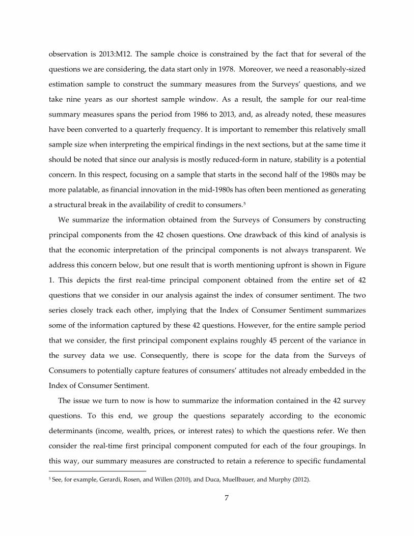
observation is 2013:M12. The sample choice is constrained by the fact that for several of the
questions we are considering, the data start only in 1978. Moreover, we need a reasonably-sized
estimation sample to construct the summary measures from the Surveys’ questions, and we
take nine years as our shortest sample window. As a result, the sample for our real-time
summary measures spans the period from 1986 to 2013, and, as already noted, these measures
have been converted to a quarterly frequency. It is important to remember this relatively small
sample size when interpreting the empirical findings in the next sections, but at the same time it
should be noted that since our analysis is mostly reduced-form in nature, stability is a potential
concern. In this respect, focusing on a sample that starts in the second half of the 1980s may be
more palatable, as financial innovation in the mid-1980s has often been mentioned as generating
a structural break in the availability of credit to consumers.5
We summarize the information obtained from the Surveys of Consumers by constructing
principal components from the 42 chosen questions. One drawback of this kind of analysis is
that the economic interpretation of the principal components is not always transparent. We
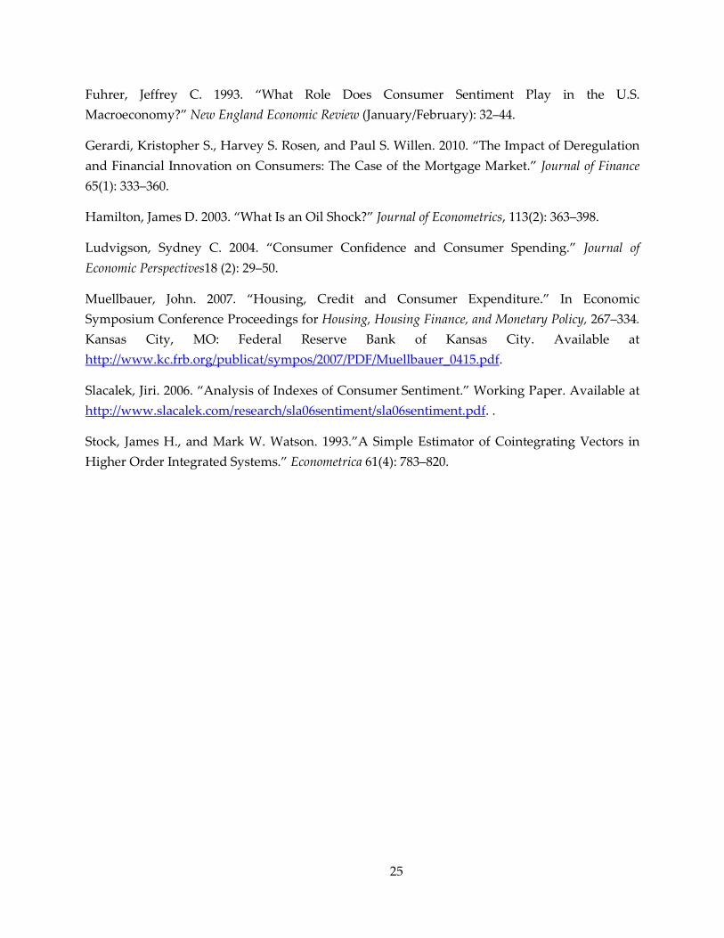
address this concern below, but one result that is worth mentioning upfront is shown in Figure
1. This depicts the first real-time principal component obtained from the entire set of 42
questions that we consider in our analysis against the index of consumer sentiment. The two
series closely track each other, implying that the Index of Consumer Sentiment summarizes
some of the information captured by these 42 questions. However, for the entire sample period
that we consider, the first principal component explains roughly 45 percent of the variance in
the survey data we use. Consequently, there is scope for the data from the Surveys of
Consumers to potentially capture features of consumers’ attitudes not already embedded in the
Index of Consumer Sentiment.
The issue we turn to now is how to summarize the information contained in the 42 survey
questions. To this end, we group the questions separately according to the economic
determinants (income, wealth, prices, or interest rates) to which the questions refer. We then
consider the real-time first principal component computed for each of the four groupings. In
this way, our summary measures are constructed to retain a reference to specific fundamental
5 See, for example, Gerardi, Rosen, and Willen (2010), and Duca, Muellbauer, and Murphy (2012).
7

determinants of consumption. This approach may prove useful if there is information in the
survey that can explain consumption, as then it will be possible to provide a somewhat more
precise economic interpretation of consumers’ attitudes.
The preliminary analysis reveals that the first principal component for the survey questions
referring to income and the first principal component for the survey questions referring to
wealth tend to be highly correlated with each other. To preserve degrees of freedom in the
analysis that follows, we jointly consider the survey questions referring to income and those
referring to wealth. This complete set comprises 25 survey questions, and the relationship
between the first principal component from these questions and a simple average of the changes
in real household income and wealth is depicted in Figure 2. From this figure it is apparent that
the real-time evolution of the principal component from the questions concerning income and
wealth captures some of the actual dynamics of households’ real income and wealth. Another
notable feature of this principal component is that it tracks consumer sentiment fairly closely.
This relationship is shown in Figure 3, which plots the principal component against consumer
sentiment, implying that consumer sentiment captures most of the elements of the survey
questions that broadly refer to income and wealth.
The first principal component is computed in real time for the eight survey questions
concerning prices, which we refer to as the prices component, and is plotted in Figure 4 against
the log real price of oil.6 This summary measure exhibits some co-movement with energy
prices.7 Additionally, it can be shown that the price component is correlated with the income
and wealth component we have just described, and thus with consumer sentiment. It is well
known that short-term fluctuations in sentiment can be driven by fluctuations in energy prices.
Given the high correlation of consumer sentiment with our real time income and wealth
component, the effect of energy prices on sentiment is presumably working via a real income
effect. However, a significant fraction of the variation in the price component is orthogonal to
6 The real price of oil is defined as the domestic crude spot oil price (West Texas intermediate) divided by the core CPI price index.
7 Fluctuations in the real price of food provide marginal additional explanatory power to the component.
8
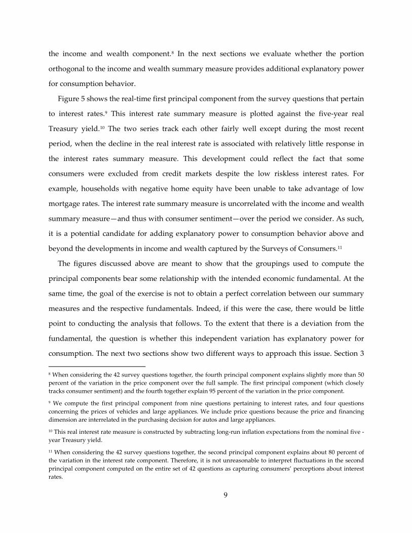
the income and wealth component.8 In the next sections we evaluate whether the portion
orthogonal to the income and wealth summary measure provides additional explanatory power
for consumption behavior.
Figure 5 shows the real-time first principal component from the survey questions that pertain
to interest rates.9 This interest rate summary measure is plotted against the five-year real
Treasury yield.10 The two series track each other fairly well except during the most recent
period, when the decline in the real interest rate is associated with relatively little response in
the interest rates summary measure. This development could reflect the fact that some
consumers were excluded from credit markets despite the low riskless interest rates. For
example, households with negative home equity have been unable to take advantage of low
mortgage rates. The interest rate summary measure is uncorrelated with the income and wealth
summary measure—and thus with consumer sentiment—over the period we consider. As such,
it is a potential candidate for adding explanatory power to consumption behavior above and
beyond the developments in income and wealth captured by the Surveys of Consumers.11
The figures discussed above are meant to show that the groupings used to compute the
principal components bear some relationship with the intended economic fundamental. At the
same time, the goal of the exercise is not to obtain a perfect correlation between our summary
measures and the respective fundamentals. Indeed, if this were the case, there would be little
point to conducting the analysis that follows. To the extent that there is a deviation from the
fundamental, the question is whether this independent variation has explanatory power for
consumption. The next two sections show two different ways to approach this issue. Section 3
8 When considering the 42 survey questions together, the fourth principal component explains slightly more than 50 percent of the variation in the price component over the full sample. The first principal component (which closely tracks consumer sentiment) and the fourth together explain 95 percent of the variation in the price component.
9 We compute the first principal component from nine questions pertaining to interest rates, and four questions concerning the prices of vehicles and large appliances. We include price questions because the price and financing dimension are interrelated in the purchasing decision for autos and large appliances.
10 This real interest rate measure is constructed by subtracting long-run inflation expectations from the nominal five -year Treasury yield.
11 When considering the 42 survey questions together, the second principal component explains about 80 percent of the variation in the interest rate component. Therefore, it is not unreasonable to interpret fluctuations in the second principal component computed on the entire set of 42 questions as capturing consumers’ perceptions about interest rates.
9
analyzes the usefulness of the summary measures for predicting future consumption, at the
same time controlling for lagged fundamentals, while section 4 performs a Campbell-Mankiw
type exercise where the usefulness of these measures to predict future consumption is gauged
in a context where we explicitly control for future fundamentals.
3. Forecasting Consumption Using the Surveys of Consumers
We now turn to examining the forecasting power of our three real-time summary
components for the dynamics of consumption growth. There is an extensive literature on the
predictive power of sentiment for consumption growth, but so far there is little work on the
predictive power of the information available in the broader Surveys of Consumers. We
consider the period from 1986:Q3 to 2013:Q4, and also examine the subsample that ends in
2007:Q4, before the onset of the last recession. We predict the growth in consumption over the
next quarter and over the next four quarters. For the regressions involving four-quarter
consumption growth, it is important to keep in mind that the number of independent
observations is limited.
We begin by assessing the explanatory power of our real-time summary measures from the
Surveys of Consumers in isolation and compare this performance with using consumer
sentiment in a real-time prediction exercise. The top panel of Table 1A shows the adjusted R2 in
regressions forecasting one-quarter-ahead personal consumption expenditures growth with two
lags of each of the three real-time measures based on the Surveys of Consumers that we
consider. The summary measure for prices is included as a first difference, since such a
restriction is not rejected by the data. The first column in the table reports the regression fit
when consumption is predicted by consumer sentiment alone, replicating and updating
findings in the extant literature. The second column shows the forecasting power of the three
summary measures from the survey—the income and wealth component, the price component,
and the interest rate component. The third column provides the regression results when both
consumer sentiment and the three summary measures from the Surveys of Consumers are used
as predictors. The bottom panel of the table performs the same exercise as used for the results
shown in the top panel, but the dependent variable is now the growth in real private
10
consumption expenditures measured over the next four quarters. Table 1A reports the results
for the whole sample whereas Table 1B reports the same results for the pre-2008 sample.12
The main message from the two tables is that there is information in the broader Surveys that
can be used to forecast consumption in real time above and beyond the information captured by
the Index of Consumer Sentiment. The adjusted R2s in the regressions where the three real-time
survey summary measures are included (the second column) rises noticeably compared to the
benchmark regressions where consumer sentiment is the only predictor for consumption (the
first column). It is also the case that when the summary measures are used as predictors,
including consumer sentiment as an additional predictor (the third column) does not improve
the predictability of consumption when growth is measured on a one-quarter basis. There is
some improvement in fit when consumption growth is measured on a four-quarter basis in the
shorter sample period, but these results could be affected by the small sample. As already
shown, the income and wealth summary measure and consumer sentiment are highly
correlated, and thus the lack of consistent improvement in fit when sentiment is added as a
predictor is not surprising. What is important in the present context is that the price and the
interest rate components both add significant explanatory power when predicting consumption
growth, regardless of the time horizon over which consumption growth is being measured.
While the analysis has been carried out on total consumption, the results in the previous
table also hold when considering the decomposition of consumption into expenditures on
durables, nondurables, and services. Table 2 reports the results for these consumption
categories over the full sample with the dependent variables expressed in terms of one-quarter-
ahead growth rates. Table 3 reports the results from performing the same exercise with the
dependent variables expressed in terms of four-quarter-ahead growth rates. It is apparent that
there is some improvement in fit when considering the real-time survey summary measures
relative to the forecasts generated with the information just contained in consumer sentiment
alone. Similar findings (not reported) hold for the pre-2008 sample.
12 A similar analysis is performed in a related exercise by Barnes and Olivei (2013), except that the analysis is not performed in real time.
11
Having established that the summary measures from the Surveys of Consumers contain
information that is useful for forecasting consumption, we now turn to assessing how much of
the predictive content is preserved when controlling for standard consumption fundamentals.
This determination is especially important in the current context, as we constructed the
summary measures from the Surveys of Consumers with reference to broad economic
categories representing different drivers of consumption behavior. It is possible that when
controlling explicitly for these predictors, our summary measures become redundant. On the
other hand, the measures could still capture features, such as animal spirits and the subjective
perceptions of economic outcomes, which help to explain consumer behavior above and beyond
the observed economic fundamentals.
Table 4 reports the adjusted R2s for regressions that forecast the growth in total consumption
expenditures while controlling for fundamentals and shows the improvement in fit when either
lags of consumer sentiment or lags of the three real-time summary measures are added to the
regressions. The fundamentals we include are two lags each of the quarterly growth rate in
consumption, real labor income as defined in Carroll, Fuhrer and Wilcox (1994),13 households’
real net worth, real oil price inflation, the level of the real interest rate (measured as the five-
year nominal Treasury yield less long-run inflation expectations), and banks’ willingness to
make consumer installment loans, a measure obtained from the Federal Reserve Board’s Senior
Loan Officer Opinion Survey on Banking Lending Practices. Controlling for the discrepancy
between the level of consumption and the level predicted from income and net worth—a
cointegrating error that captures deviations from the long-run relationship between
consumption and fundamentals—does not alter the results. The table’s first column shows the
adjusted R2s with only the standard fundamentals just described. The second column reports
the goodness of fit when these fundamentals are augmented by the inclusion of two lags of
consumer sentiment. The third column reports the results when these fundamentals are
13 Real labor income is defined to be real wages, salaries, and transfers less personal contributions for social insurance. This measure differs from disposable income in that it excludes other labor income such as employer contributions for pension and benefit plans in addition to interest, dividend, rental, and proprietor’s income. It also does not deduct personal tax and nontax payments. As argued in Carroll, Fuhrer, and Wilcox (1994), the tax data can be dominated by changes in payments largely available to, and used by, higher-income households.
12
augmented with the three summary components from the Surveys, where each component is
entered with two lags. When controlling for these components, we do not include sentiment as
an additional explanatory variable, as sentiment and the income and wealth component
essentially convey the same information. The exercise is also repeated for the pre-2008 sample
(not shown).
Comparing the fit between the first and second columns shows, similar to previous results in
the literature, that once the fundamentals are controlled for, the role of consumer sentiment in
predicting consumption is marginal at best. Instead, there is a significant improvement in fit
when the Surveys’ summary measures are added to the fundamentals. As shown in the bottom
panel of Table 4, these findings also hold when consumption growth is measured over a four-
quarter-ahead horizon. The same pattern of findings (not reported) emerges when evaluating
the different components of consumption. Overall, there appears to be explanatory power in the
real-time components from the Surveys of Consumers that goes beyond the observed
fundamentals. The relative statistical significance of the three summary measures can vary
according to the set of fundamentals included in the forecasting regressions. However, the
interest rate component is typically an important contributor to the improvement in fit.
4. Consumption Behavior and the Surveys of Consumers: An Augmented Campbell-Mankiw Framework
An important issue is to what extent our summary measures from the Surveys have
predictive power for consumption growth because these measures can forecast future
developments in household income, household net worth, and credit availability. In the simple
version of the permanent income hypothesis, changes in consumption are solely a function of
innovations to permanent income. However, if a portion of households follow a rule of thumb
whereby every period they consume a certain fraction of their income (Campbell and Mankiw
1989, 1990), or if a portion of consumers are credit constrained, then contemporaneous changes
in consumption can be associated with contemporaneous changes in income, household net
worth, and credit availability. It is thus relevant to assess whether the summary measures’
13
ability to predict consumption arises from their forecasting power for these fundamentals, or
from another independent channel.
The first step in testing this hypothesis is to check the extent to which the summary measures
have forecasting power for household income, net worth, and credit availability. If the
summary measures are uncorrelated with these fundamentals, then the previous section’s
assessment of the ability of the summary measures to forecast consumption would be unbiased.
Table 5 reports the results of forecasting regressions where the dependent variables are labor
income,14 household stock market wealth, household wealth excluding stock market wealth,
and credit conditions. The sample period is 1986:Q3 to 2013:Q4. The first three variables are
expressed in growth rates, while the credit conditions variable is taken from the Senior Loan
Officer Opinion Survey, which measures banks’ willingness to make consumer installment
loans relative to three months earlier. Given that this variable is already defined as a change, no
transformation is needed.
The table compares the adjusted 2R statistics once the simple autoregressive forecasting
regressions are augmented with lags of the summary measures. The baseline forecasting
regressions include two lags of the dependent variable. In the augmented regressions, we use
two lags of each of the summary measures, with the price measure constrained to enter as a first
difference. The values in parenthesis are p-values from a Wald test on the joint significance of
the summary measures in the augmented specification. Introducing the summary measures
increases the adjusted 2R only when the dependent variable is either labor income or credit
availability. In those two cases, the increment in the adjusted 2R is near 7 percent. The Wald test
indicates the hypothesis that the summary measures have no forecasting power can be rejected
at the 2 percent level or less. For the household wealth variables, represented either by stock
market wealth or non-stock market wealth, the summary measures provide no additional
forecasting power over the sample we consider.
Given these findings, in what follows we consider a consumption specification that controls
only for contemporaneous changes in labor income and credit conditions. In particular, by
14 The labor income variable is defined as in the previous section and according to Carroll, Fuhrer, and Wilcox (1994). For the definition and a motivation for how the variable is constructed, see footnote 12.
14
expanding on the specification of Carroll, Fuhrer, and Wilcox (1994), we estimate the following
relationship:
(1) 1't t t t tC Y FWILLλ γ ν ϑν −∆ = ∆ + + + −t-1β X ,
where C is real total consumption expenditures, Y is labor income, and FWILL is banks’
willingness to make consumer installment loans in the current period relative to three months
earlier. The operator ∆ computes the quarterly annualized percentage change for the variable
to which it is applied. The vector of variables X contains the lagged summary measures from
the Surveys of Consumers. In this exercise, we do not include lagged consumer sentiment—the
focus of the Carroll, Fuhrer, and Wilcox analysis—as we have shown that sentiment is highly
correlated with our income and wealth summary measure. Our setup augments the Campbell-
Mankiw framework by allowing changes in consumption to be affected not just by rule-of-
thumb behavior, but also by the presence of credit-dependent households whose consumption
can vary according to changes in credit availability. The specification explicitly features an
MA(1) error term to account for time aggregation in the measurement of consumption
(Christiano, Eichenbaum, and Marshall, 1991).
Since Y and FWILL enter the regression contemporaneously, the endogeneity issue is
addressed by means of instrumental variable estimation. Moreover, the explicit estimation of
the MA(1) error term in the regression implies that instruments dated t–1 and earlier are
permissible. The set of instruments is comprised of a constant and three lags each of the C∆ ,
Y∆ , FWILL , the unemployment rate, the real interest rate, the risk premium, and inflation. The
real interest rate, as in the previous section, is given by the difference between the five-year
Treasury nominal yield and an estimate of long-run inflation expectations.15 The risk premium
is defined as the difference between the yield on BAA-rated corporate bonds and the 10-year
Treasury yield, while inflation is the quarterly annualized percentage change in the PCE
deflator.
The estimation results are reported in Table 6 for the same sample period, 1986:Q3 to
2013:Q4. Column (1) provides estimates of equation (2) without including X , the lagged
15 The long-run measure of inflation expectations is taken from the Hoey/Philadelphia Survey of Professional Forecasters.
15
summary measures. The estimate for the rule-of-thumb parameter λ is insignificant, while the
credit availability measure is highly significant and economically meaningful. A 10 percentage
point increase in FWILL raises consumption by roughly seven-tenths of a percentage point at
an annual rate.16 This insignificance of the rule-of-thumb parameter contrasts with estimates
obtained in previous studies on earlier sample periods. However, the estimated responsiveness
of consumption to income changes when the first lag of the change in income is included as an
additional regressor. These results are shown in column (2), where now both the
contemporaneous and the lagged change in income are significant. The sum of these coefficients
is estimated at 0.50. One interpretation of this finding is that rule-of-thumb consumers respond
to contemporaneous and lagged income. Another interpretation, which is that lagged income
growth is proxying for consumption habits, does not find support over this specific sample
period. The estimation results in column (3) show that the inclusion of lagged consumption
growth neither adds explanatory power nor materially alters the previous finding about the
relevance of lagged income growth.
In Table 6, Column (4) shows the regression results obtained from augmenting the
specification in the second column by including the three summary measures from the Surveys
of Consumers. We include two lags of these measures, with the prices component constrained
to enter the relationship in first differences. The column also reports test results for the sum of
the estimated coefficients for current and lagged income growth, and for the sum of the
coefficients for the two lags, respectively, of the income and wealth and the interest rate
components. With respect to the income and credit availability fundamentals, controlling for
the summary measures does not alter the economic significance of current and lagged changes
in income, but slightly weakens the significance of the change in current credit conditions.
Comparing the estimated coefficients for the summary measures with those from column (5),
where we consider only the summary measures as explanatory variables, reveals the degree to
which the predictive ability of the summary measures is independent of their ability to predict
the fundamentals that matter for future consumption growth. Relative to the estimates in
16 The variable FWILL measures the net percentage of bank respondents who are willing to increase consumer installment loans relative to three months earlier.
16
column (5), the test of the sum of the coefficients on the income and wealth component yields a
sum that is roughly half the size of that in the regression that does not control for fundamentals,
and it is less precisely estimated. In addition, the economic and statistical significance of the first
difference of the prices component diminishes somewhat. In contrast, the sum of the coefficients
on the interest rate component becomes both more economically significant and more precisely
estimated when controlling for income and credit fundamentals. Still, the overall implication of
these findings is that while the summary measures predict future consumption growth partly
because of their ability to predict real income growth and credit conditions, they retain an
independent predictive power. These findings are along the lines of the results in Carroll,
Fuhrer, and Wilcox (1994) for consumer sentiment, though our focus is broader as some of the
informational content from the Surveys of Consumers that we consider is orthogonal to
consumer sentiment. This is especially true for the interest rate component, which contributes
significantly to the Surveys’ independent explanatory power for future consumption growth.
The results in this and in the previous section illustrate that there is information in the
Surveys of Consumers that helps to predict consumption growth above and beyond
fundamentals. Yet these findings could still be driven by the omission of relevant economic
developments. For this reason, in the next section we consider the extent to which the survey
information is incorporated efficiently into professional forecasts of economic activity, which
are likely conditioned on a broader set of fundamentals than the one we have considered here.
Moreover, these professional forecasts contain a judgmental component that could capture
animal spirits or other features of the economic environment. These features are hard to
measure and could be correlated with the portion of the Surveys’ summary measures that is
orthogonal to fundamentals.
5. The Informational Content of the Surveys of Consumers for Professional Forecasters
In this section, we consider whether the summary measures we derive from the Surveys of
Consumers can explain errors in the Survey of Professional Forecasters’ (SPF) and the Federal
Reserve Board’s Greenbook forecasts of real consumption growth. We also present results
pertaining to forecast errors in real GDP growth and in the level of the unemployment rate in
17
order to assess the importance of the summary measures for forecasting broader economic
developments, as well as to explore channels other than consumption through which this
information may be relevant.
For current-quarter forecasts, we consider the SPF and Greenbook forecast errors in the context
of the following specification:
(2) 2 2 2
, ,0 1
1 1 1
E t E tt t t Yk t k Rk t k Pk t k t
k k k
X X a a X b PY b PR b PP e− − −= = =
− = + + + + +∑ ∑ ∑ .
In this equation, X denotes the variable that is being forecast (real consumption growth, real GDP
growth, or the unemployment rate). The superscript ,E t indicates the time t forecast of variable
X with the forecast being either from the SPF or the Greenbook. The variable PY denotes the
summary measure for income and wealth, while PR and PP denote the summary measures for
interest rates and prices, respectively. The forecasters that comprise the SPF are surveyed in the
middle-month of the quarter, and we use the median forecast. For the Greenbook forecasts,
which were made eight times a year over the period we consider, we convert to a quarterly
frequency in order to align the forecasts as closely as possible with those of the SPF. This
typically means keeping the January, March, August and October Greenbook forecasts; that is,
the forecast made early in the given quarter. For year-out forecasts of real consumption and
GDP growth, the previous equation is modified as follows:
(3) 2 2 2
, ,4, 3 4, 3 0 1 4, 3
1 1 1
E t E tt t t Yk t k Rk t k Pk t k t
k k k
X X a a b PY b bX PR PP e+ + + − − −= = =
− = + + + + +∑ ∑ ∑ ,
where 4, 3tX + is defined as 3
4, 30
0.25*t t ii
X X+ +=
≡ ∑ . In other words, 4, 3tX + is the four-quarter change
of the variable in question over the period 1t − to 3t + . The forecast of 4, 3tX + is similarly defined
as 3
, ,4, 3
00.25*E t E t
t t ii
X X+ +=
≡ ∑ . For the level of the unemployment rate, the year-out specification
instead becomes:
(3’) 2 2 2
, ,3 3 0 1 3
1 1 1
E t E tt t t Yk t k Rk t k Pk t k t
k k k
X X a a X b PY b PR b PP e+ + + − − −= = =
− = + + + + +∑ ∑ ∑ .
18
In all of the specifications we consider, the actual value for real consumption and GDP growth
is taken to be the value measured by the Bureau of Economic Analysis (BEA) eight quarters after
the BEA’s third (or final) release. Equivalently, this is the prevailing “actual” value nine quarters
after the forecast is made. We have chosen such a definition for actual values as a compromise
between more “real-time” estimates, which are incomplete and can undergo substantial revisions,
and more distant estimates, which can encompass methodological changes that a forecaster
would not take into consideration when predicting real activity.17 For the unemployment rate, we
simply take the most recent vintage of the data because the unemployment rate—aside from
minor seasonal adjustments—is not being revised. The specifications describe the forecast errors
as a function of a constant, the forecast itself, and two lags of each summary measure from the
Surveys of Consumers. The forecast is included as an explanatory variable to account for the
possibility that it is correlated with the summary measures and that it is inefficient when
explicitly controlling for the survey information.
The regression sample begins in 1987:Q1. The sample ends in 2008:Q4 for the Greenbook
forecasts, since the Greenbook information is publicly released with a five-year lag. For the SPF
forecasts, we use information up to 2013:Q4. Given that the actual values are defined as the
values prevailing nine quarters after the forecast is being made, the current-quarter forecast
error regressions stop in 2011:Q3, while the year-out forecast error regressions stop in 2010:Q3.
When considering the year-out forecasts, the estimation takes into account the moving-average
nature of the error term.18
Tables 7 to 9 show that for all of the different forecasting errors considered (current quarter,
year-ahead; SPF or Greenbook; real consumption growth, real GDP growth, or the
unemployment rate), roughly 20 to 40 percent of the variation in the forecasting errors can be
explained by including the three summary measures from the Surveys of Consumers. In order
to illustrate the similarity of the results for both the Greenbook and SPF forecasts for the same
17 The results provided in this section are qualitatively similar when other data release “vintages” are considered, in that the additional information provided by the summary measures always yields a significant increase in the percent variation explained of the forecast error, regardless which “vintage” of the data series are taken to be the actuals.
18 Specifically, we are correcting the standard errors of the estimated parameters to account for a moving average structure of order three in the residuals.
19

sample, the tables also include the SPF results for the shorter Greenbook sample. The signs of
the estimated coefficients for the summary measures have some economic rationale as well, in
that improvements in the component capturing the income and wealth effect, as well as the
component measuring improved credit conditions and lower interest rates, are associated with
actual real activity values above those forecasted, whereas the component for prices is
associated with lower activity than forecasted, perhaps due to the effect of inflation on
disposable income. Still, there is no obvious pattern to the particular summary measures that
contribute most to explaining the variation in forecast errors. For example, the income and
wealth summary measure tends to matter for explaining unemployment rate forecast errors, but
it matters less for the two other real activity measures, for which the interest or prices summary
measures have relatively more explanatory power. From the tables, it is also apparent that once
controlling for the summary measures, the estimate for the coefficient 1a on the forecast often
becomes significantly negative. This finding implies that forecasts do not efficiently incorporate
the information from the Surveys of Consumers’ summary measures.19 Therefore, a more
efficient forecast will down-weight the Greenbook or the SPF forecast and will combine its
predictions with the summary measures.
Figures 6 to 11 visually illustrate the benefit of using information from the Surveys of
Consumers to adjust the Greenbook and SPF forecasts at the one-year horizon for the three
activity variables that we consider. For the SPF forecasts, the sample runs through 2014:Q1,
since the adjusted and unadjusted forecasts are not reliant upon the existence of the actual value
(which for real consumption and GDP growth is the value prevailing nine quarters after the
forecast is made). From these figures, it is apparent that the adjusted forecasts track the actual
values better than the unadjusted forecasts do near turning points, which are notoriously hard
to predict.
19 When one cannot reject the hypothesis that the coefficient 1a is zero even after controlling for the summary
measures, the implication is that the information in the summary measures, while explaining variation in the forecast error, is not significantly correlated with the forecast. This case, however, does not occur for the year-out forecasts, where the forecasts and the information in the summary measures exhibit correlation. In contrast, for the current-quarter forecasts, the correlation tends to be much less pronounced.
20
As discussed, for real consumption and GDP growth, we have chosen actual values in the
forecast error regressions that, being two years removed from the third BEA release, allow for
some revisions to the data. The issue then turns to what extent the information contained in the
Surveys of Consumers’ summary measures do improve professional forecasts—whether simply
through an ability to predict data revisions or because the informational content goes beyond this
predictability. It can be shown that the summary measures have some predictive power for data
revisions—when the revisions are defined as the difference between the value that prevails two
years after the third BEA release, and the third release. This is especially true for real consumption
growth, whereas for real GDP growth the summary measures’ predictive power is marginal.20 We
thus augment the previous forecast error regressions by controlling for the two-years-out revision
to the third release, meaning REV RTt t tX X X≡ − , where we keep the previous notation for tX as
representing the actual value for variable X (either real consumption or GDP growth) that
prevails at time t as measured and released by the BEA two years after the third release, RTtX . As
already mentioned, this exercise is not necessary for the unemployment rate, which does not get
revised.
Tables 10 and 11 report the estimation results for the forecast error regressions when
controlling for REVtX . Overall, the findings are qualitatively similar to those shown in the previous
tables. The summary measures from the Surveys of Consumers continue to have predictive power
for forecast errors, with the signs of the estimated coefficients maintaining a sensible economic
interpretation. While forecasters do not have the benefit of knowing future data revisions at the
time they make their forecasts, the findings are consistent with the idea that the summary
measures contain information useful for improving forecasts of real economic activity above and
beyond their ability to predict revisions to the data being forecasted.
6. Conclusions
20 These results are available from the authors upon request; this result also holds for the one- and three-years-out revisions of the third BEA release.
21
We have shown that the Reuters/Michigan Surveys of Consumers contain information about
future aggregate consumption behavior that is not embedded in standard economic
determinants of consumer spending. This information goes beyond the predictive power of
consumer sentiment for consumption growth, which already has been widely documented in
the literature. Considering information in the survey orthogonal to consumer sentiment
provides additional explanatory power when forecasting aggregate real consumption growth,
even when controlling for standard consumption fundamentals. The forecasting power from the
survey still remains when considering a rule-of-thumb specification of consumption behavior or
credit-dependent consumers.
While it is possible that we have not adequately captured the relevant measures of economic
fundamentals—for example, in some exercises we control for a risk-free real interest rate which
is only correlated with the relevant cost of credit faced by consumers—we have also shown that
the information in the Surveys of Consumers helps to reduce errors in the Survey of
Professional Forecasters and in the Greenbook forecasts of real consumption and other
measures of real economic activity. Presumably, such forecasts control for a broader set of
fundamentals than we have considered, and yet the reduction in the forecast errors that come
from including the summary information from the Surveys can be noticeable. Still, the
possibility of not including or mismeasuring a relevant fundamental cannot be ruled out
entirely, as the forecasts are not always factoring in the relevant fundamentals in an efficient
manner. For example, it has been shown that over much of the sample period we consider, the
Survey of Professional Forecasters and the Greenbook forecasts were not efficiently
incorporating information on economic activity related to credit availability as gauged by the
Senior Loan Officer Opinion Survey (Barnes 2014).
It is often argued that deviations of consumer attitudes from fundamental determinants of
consumption may reflect uncertainty surrounding the economic environment. Still, recasting
the findings in terms of uncertainty as providing the “missing” fundamental is not
straightforward, as already pointed out in the literature (Carroll, Fuhrer, and Wilcox 1994). If,
for example, our summary measure for consumers’ current attitudes toward income and wealth
is low due to an uncertain environment, consumption growth should be higher in the future as
22
this uncertainty dissipates. This situation would generate a negative relationship between
future consumption growth and our summary measure, rather than the positive relationship
found in the data.
While the explanation for why consumer attitudes help forecast consumption remains
unclear, this study offers some understanding in terms of the type of consumer attitudes that
provide the forecasting power. Consumer attitudes that broadly relate to income and wealth
developments matter. These attitudes are also captured by the consumer sentiment index, and
in this respect the forecasting power for consumption is, therefore, not too surprising. However,
consumer attitudes regarding interest rates and credit availability, which over the period we
consider provide information that is largely orthogonal to consumer sentiment, also have
forecasting power. This is also the case for consumer attitudes towards prices, whose relevance
for forecasting consumption while controlling for consumers’ attitudes toward income and
wealth could reflect the low short-run price elasticity of certain items, such as energy-related
goods and services. Further distinguishing between attitudes towards present conditions and
expectations about future conditions is a potential extension of this analysis.
The information from the Surveys that is summarized by our principal components is
generally significant from a statistical standpoint, but its economic relevance is apparent only
occasionally. With the inclusion of these summary measures, a sizable portion of the variation
in consumption growth still remains unexplained even if the summary measures’ explanatory
power is noticeably larger than that of consumer sentiment. Yet a consideration of some of these
measures appears to be of consequence in certain episodes. For example, our analysis of forecast
errors in the previous section illustrates how efficiently incorporating the information from the
Surveys could have appreciably lowered the forecast errors during the second half of the 1990s
and during the Great Recession. Information from the Surveys could also prove useful at the
current juncture. With the waning of the restraining effects of fiscal policy on households’
income and a sizable appreciation in net worth, real consumption growth is expected to
accelerate over the course of 2014. The extent of such acceleration, however, can be affected by
credit conditions. In this respect, the Surveys of Consumers provide a somewhat more
23

pessimistic assessment of credit conditions than simple readings of the level of the real interest
rate, which remains very low by historical standards.
References
Barnes, Michelle L.Forthcoming. “What Kind of Finance Matters for Forecast Errors?” Working Paper . Boston: Federal Reserve Bank of Boston.
Barnes, Michelle L., and Giovanni P. Olivei. 2013. “The Michigan Surveys of Consumers and Consumer Spending.” Public Policy Brief No. 13-2. Boston: Federal Reserve Bank of Boston. Available at https://www.bostonfed.org/economic/ppb/2013/ppb138.pdf.
Brayton, Flint, Morris Davis, and Peter Tulip. 2000. “Polynomial Adjustment Costs in FRB/US.” Unpublished Note. Available at http://petertulip.com/pacmay2000.pdf.
Campbell, John Y., and Gregory N. Mankiw. 1989. “Consumption, Income, and Interest Rates: Reinterpreting the Time Series Evidence.” In NBER Macroeconomics Annual 1989, eds. Olivier J. Blanchard and Stanley Fischer, pp. 185–216. Cambridge, MA: The MIT Press.
Campbell, John Y., and Gregory N. Mankiw. 1990. “Permanent Income, Current Income, and Consumption.” Journal of Business and Economic Statistics 8(3): 265–279.
Carroll, Christopher D., Jeffrey C. Fuhrer, and David W. Wilcox. 1994. “Does Consumer Sentiment Forecast Household Spending? If So, Why?” American Economic Review 84(5): 1397–1408.
Carroll, Christopher D., Jiri Slacalek, and Martin Sommer. 2012. “Dissecting Saving Dynamics: Measuring Wealth, Precautionary, and Credit Effects.” IMF Working Paper No. 219. Washing-ton, DC: International Monetary Fund. Available at https://www.imf.org/external/pubs/ft/wp/2012/wp12219.pdf.
Christiano, Lawrence J., Martin Eichenbaum, and David Marshall. 1991. “The Permanent Income Hypothesis Revisited.” Econometrica 59(2): 397–423.
Duca, John V., John Muellbauer, and Anthony Murphy. 2010. “Credit Market Architecture and the Boom and Bust in U.S. Consumption.” Working Paper. Available at https://editorialexpress.com/cgibin/conference/download.cgi?db_name=res2011&paper_id=1213
Duca, John V., John Muellbauer, and Anthony Murphy. 2012. “How Financial Innovations and Accelerators Drive Booms and Busts in U.S. Consumption.” Working Paper. Available at https://www.stlouisfed.org/household-financial-stability/events/20130205/papers/Duca.pdf.
24
Fuhrer, Jeffrey C. 1993. “What Role Does Consumer Sentiment Play in the U.S. Macroeconomy?” New England Economic Review (January/February): 32–44.
Gerardi, Kristopher S., Harvey S. Rosen, and Paul S. Willen. 2010. “The Impact of Deregulation and Financial Innovation on Consumers: The Case of the Mortgage Market.” Journal of Finance 65(1): 333–360.
Hamilton, James D. 2003. “What Is an Oil Shock?” Journal of Econometrics, 113(2): 363–398.
Ludvigson, Sydney C. 2004. “Consumer Confidence and Consumer Spending.” Journal of Economic Perspectives18 (2): 29–50.
Muellbauer, John. 2007. “Housing, Credit and Consumer Expenditure.” In Economic Symposium Conference Proceedings for Housing, Housing Finance, and Monetary Policy, 267–334. Kansas City, MO: Federal Reserve Bank of Kansas City. Available at http://www.kc.frb.org/publicat/sympos/2007/PDF/Muellbauer_0415.pdf.
Slacalek, Jiri. 2006. “Analysis of Indexes of Consumer Sentiment.” Working Paper. Available at http://www.slacalek.com/research/sla06sentiment/sla06sentiment.pdf. .
Stock, James H., and Mark W. Watson. 1993.”A Simple Estimator of Cointegrating Vectors in Higher Order Integrated Systems.” Econometrica 61(4): 783–820.
25
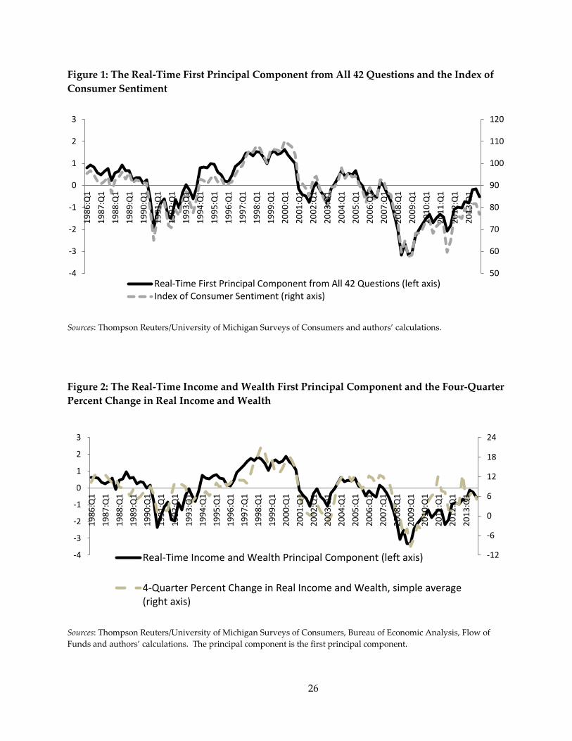
Figure 1: The Real-Time First Principal Component from All 42 Questions and the Index of Consumer Sentiment
Sources: Thompson Reuters/University of Michigan Surveys of Consumers and authors’ calculations.
Figure 2: The Real-Time Income and Wealth First Principal Component and the Four-Quarter Percent Change in Real Income and Wealth
Sources: Thompson Reuters/University of Michigan Surveys of Consumers, Bureau of Economic Analysis, Flow of Funds and authors’ calculations. The principal component is the first principal component.
50
60
70
80
90
100
110
120
-4
-3
-2
-1
0
1
2
3
1986
:Q1
1987
:Q1
1988
:Q1
1989
:Q1
1990
:Q1
1991
:Q1
1992
:Q1
1993
:Q1
1994
:Q1
1995
:Q1
1996
:Q1
1997
:Q1
1998
:Q1
1999
:Q1
2000
:Q1
2001
:Q1
2002
:Q1
2003
:Q1
2004
:Q1
2005
:Q1
2006
:Q1
2007
:Q1
2008
:Q1
2009
:Q1
2010
:Q1
2011
:Q1
2012
:Q1
2013
:Q1
Real-Time First Principal Component from All 42 Questions (left axis)Index of Consumer Sentiment (right axis)
-12
-6
0
6
12
18
24
-4
-3
-2
-1
0
1
2
3
1986
:Q1
1987
:Q1
1988
:Q1
1989
:Q1
1990
:Q1
1991
:Q1
1992
:Q1
1993
:Q1
1994
:Q1
1995
:Q1
1996
:Q1
1997
:Q1
1998
:Q1
1999
:Q1
2000
:Q1
2001
:Q1
2002
:Q1
2003
:Q1
2004
:Q1
2005
:Q1
2006
:Q1
2007
:Q1
2008
:Q1
2009
:Q1
2010
:Q1
2011
:Q1
2012
:Q1
2013
:Q1
Real-Time Income and Wealth Principal Component (left axis)
4-Quarter Percent Change in Real Income and Wealth, simple average(right axis)
26
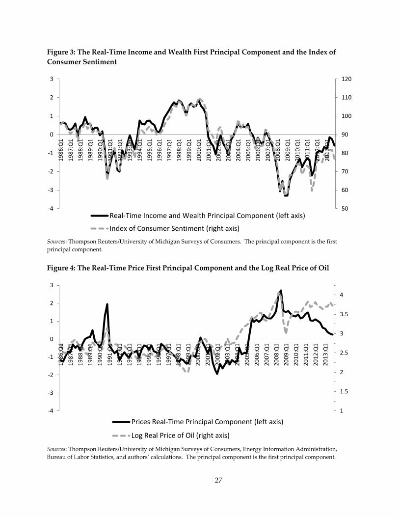
Figure 3: The Real-Time Income and Wealth First Principal Component and the Index of Consumer Sentiment
Sources: Thompson Reuters/University of Michigan Surveys of Consumers. The principal component is the first principal component. Figure 4: The Real-Time Price First Principal Component and the Log Real Price of Oil
Sources: Thompson Reuters/University of Michigan Surveys of Consumers, Energy Information Administration, Bureau of Labor Statistics, and authors’ calculations. The principal component is the first principal component.
50
60
70
80
90
100
110
120
-4
-3
-2
-1
0
1
2
3
1986
:Q1
1987
:Q1
1988
:Q1
1989
:Q1
1990
:Q1
1991
:Q1
1992
:Q1
1993
:Q1
1994
:Q1
1995
:Q1
1996
:Q1
1997
:Q1
1998
:Q1
1999
:Q1
2000
:Q1
2001
:Q1
2002
:Q1
2003
:Q1
2004
:Q1
2005
:Q1
2006
:Q1
2007
:Q1
2008
:Q1
2009
:Q1
2010
:Q1
2011
:Q1
2012
:Q1
2013
:Q1
Real-Time Income and Wealth Principal Component (left axis)
Index of Consumer Sentiment (right axis)
1
1.5
2
2.5
3
3.5
4
-4
-3
-2
-1
0
1
2
3
1986
:Q1
1987
:Q1
1988
:Q1
1989
:Q1
1990
:Q1
1991
:Q1
1992
:Q1
1993
:Q1
1994
:Q1
1995
:Q1
1996
:Q1
1997
:Q1
1998
:Q1
1999
:Q1
2000
:Q1
2001
:Q1
2002
:Q1
2003
:Q1
2004
:Q1
2005
:Q1
2006
:Q1
2007
:Q1
2008
:Q1
2009
:Q1
2010
:Q1
2011
:Q1
2012
:Q1
2013
:Q1
Prices Real-Time Principal Component (left axis)
Log Real Price of Oil (right axis)
27
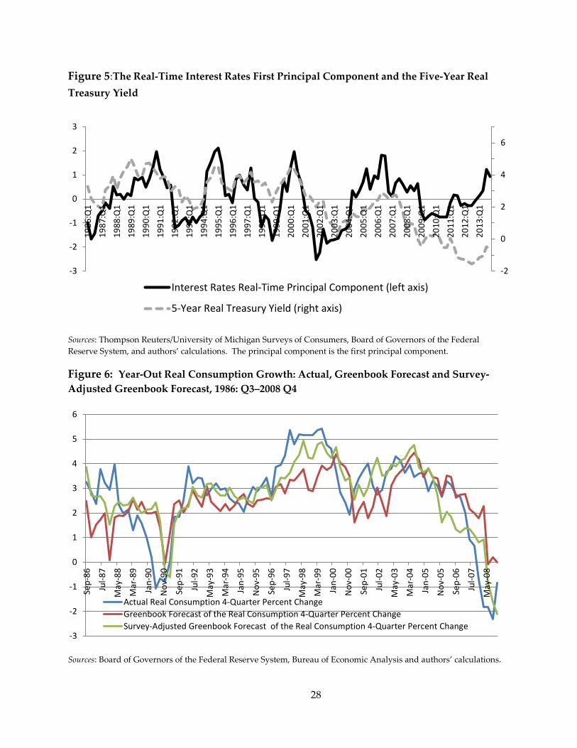
Figure 5:The Real-Time Interest Rates First Principal Component and the Five-Year Real Treasury Yield
Sources: Thompson Reuters/University of Michigan Surveys of Consumers, Board of Governors of the Federal Reserve System, and authors’ calculations. The principal component is the first principal component.
Figure 6: Year-Out Real Consumption Growth: Actual, Greenbook Forecast and Survey-Adjusted Greenbook Forecast, 1986: Q3–2008 Q4
Sources: Board of Governors of the Federal Reserve System, Bureau of Economic Analysis and authors’ calculations.
-2
0
2
4
6
-3
-2
-1
0
1
2
3
1986
:Q1
1987
:Q1
1988
:Q1
1989
:Q1
1990
:Q1
1991
:Q1
1992
:Q1
1993
:Q1
1994
:Q1
1995
:Q1
1996
:Q1
1997
:Q1
1998
:Q1
1999
:Q1
2000
:Q1
2001
:Q1
2002
:Q1
2003
:Q1
2004
:Q1
2005
:Q1
2006
:Q1
2007
:Q1
2008
:Q1
2009
:Q1
2010
:Q1
2011
:Q1
2012
:Q1
2013
:Q1
Interest Rates Real-Time Principal Component (left axis)
5-Year Real Treasury Yield (right axis)
-3
-2
-1
0
1
2
3
4
5
6
Sep-
86
Jul-8
7
May
-88
Mar
-89
Jan-
90
Nov
-90
Sep-
91
Jul-9
2
May
-93
Mar
-94
Jan-
95
Nov
-95
Sep-
96
Jul-9
7
May
-98
Mar
-99
Jan-
00
Nov
-00
Sep-
01
Jul-0
2
May
-03
Mar
-04
Jan-
05
Nov
-05
Sep-
06
Jul-0
7
May
-08
Actual Real Consumption 4-Quarter Percent ChangeGreenbook Forecast of the Real Consumption 4-Quarter Percent ChangeSurvey-Adjusted Greenbook Forecast of the Real Consumption 4-Quarter Percent Change
28
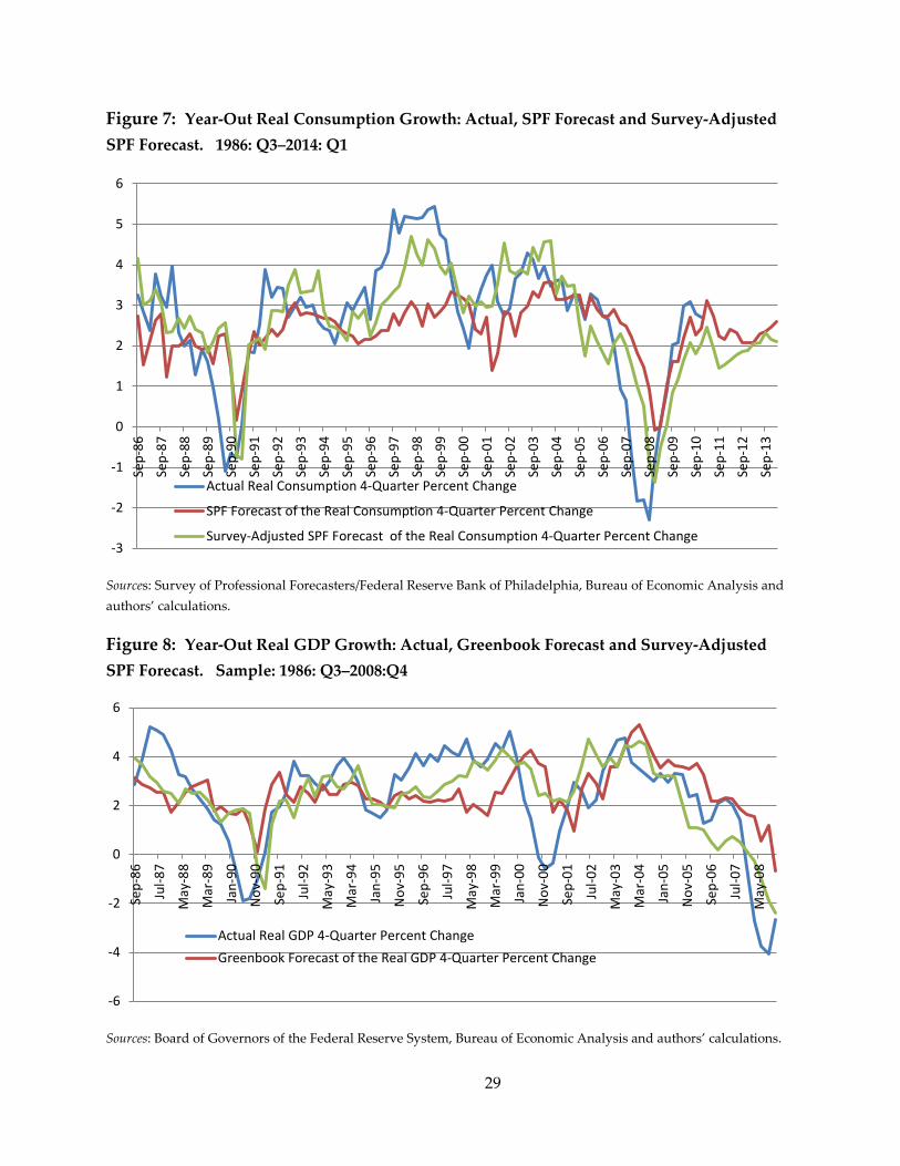
Figure 7: Year-Out Real Consumption Growth: Actual, SPF Forecast and Survey-Adjusted SPF Forecast. 1986: Q3–2014: Q1
Sources: Survey of Professional Forecasters/Federal Reserve Bank of Philadelphia, Bureau of Economic Analysis and authors’ calculations.
Figure 8: Year-Out Real GDP Growth: Actual, Greenbook Forecast and Survey-Adjusted SPF Forecast. Sample: 1986: Q3–2008:Q4
Sources: Board of Governors of the Federal Reserve System, Bureau of Economic Analysis and authors’ calculations.
-3
-2
-1
0
1
2
3
4
5
6
Sep-
86
Sep-
87
Sep-
88
Sep-
89
Sep-
90
Sep-
91
Sep-
92
Sep-
93
Sep-
94
Sep-
95
Sep-
96
Sep-
97
Sep-
98
Sep-
99
Sep-
00
Sep-
01
Sep-
02
Sep-
03
Sep-
04
Sep-
05
Sep-
06
Sep-
07
Sep-
08
Sep-
09
Sep-
10
Sep-
11
Sep-
12
Sep-
13
Actual Real Consumption 4-Quarter Percent Change
SPF Forecast of the Real Consumption 4-Quarter Percent Change
Survey-Adjusted SPF Forecast of the Real Consumption 4-Quarter Percent Change
-6
-4
-2
0
2
4
6
Sep-
86
Jul-8
7
May
-88
Mar
-89
Jan-
90
Nov
-90
Sep-
91
Jul-9
2
May
-93
Mar
-94
Jan-
95
Nov
-95
Sep-
96
Jul-9
7
May
-98
Mar
-99
Jan-
00
Nov
-00
Sep-
01
Jul-0
2
May
-03
Mar
-04
Jan-
05
Nov
-05
Sep-
06
Jul-0
7
May
-08
Actual Real GDP 4-Quarter Percent ChangeGreenbook Forecast of the Real GDP 4-Quarter Percent Change
29
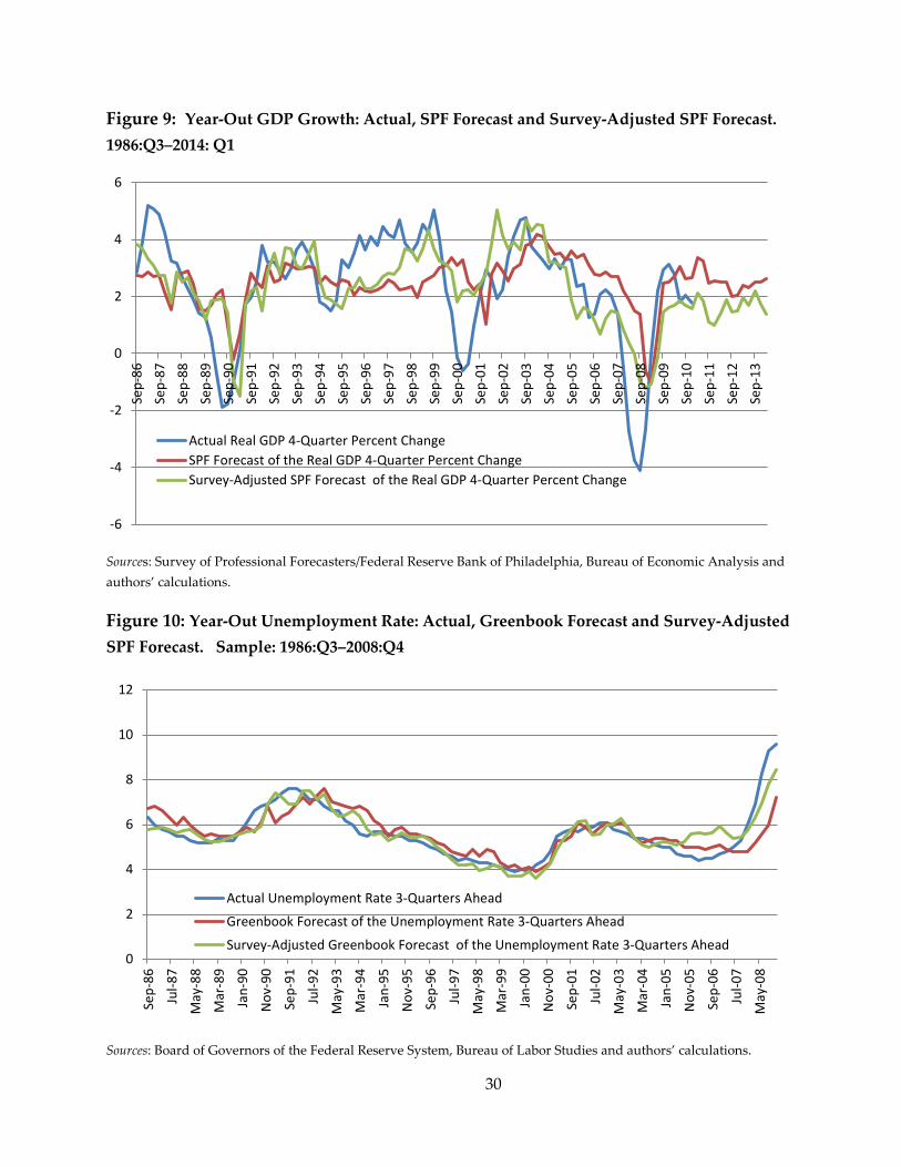
Figure 9: Year-Out GDP Growth: Actual, SPF Forecast and Survey-Adjusted SPF Forecast. 1986:Q3–2014: Q1
Sources: Survey of Professional Forecasters/Federal Reserve Bank of Philadelphia, Bureau of Economic Analysis and authors’ calculations.
Figure 10: Year-Out Unemployment Rate: Actual, Greenbook Forecast and Survey-Adjusted SPF Forecast. Sample: 1986:Q3–2008:Q4
Sources: Board of Governors of the Federal Reserve System, Bureau of Labor Studies and authors’ calculations.
-6
-4
-2
0
2
4
6
Sep-
86Se
p-87
Sep-
88Se
p-89
Sep-
90Se
p-91
Sep-
92Se
p-93
Sep-
94Se
p-95
Sep-
96Se
p-97
Sep-
98Se
p-99
Sep-
00Se
p-01
Sep-
02Se
p-03
Sep-
04Se
p-05
Sep-
06Se
p-07
Sep-
08Se
p-09
Sep-
10Se
p-11
Sep-
12Se
p-13
Actual Real GDP 4-Quarter Percent ChangeSPF Forecast of the Real GDP 4-Quarter Percent ChangeSurvey-Adjusted SPF Forecast of the Real GDP 4-Quarter Percent Change
0
2
4
6
8
10
12
Sep-
86
Jul-8
7
May
-88
Mar
-89
Jan-
90
Nov
-90
Sep-
91
Jul-9
2
May
-93
Mar
-94
Jan-
95
Nov
-95
Sep-
96
Jul-9
7
May
-98
Mar
-99
Jan-
00
Nov
-00
Sep-
01
Jul-0
2
May
-03
Mar
-04
Jan-
05
Nov
-05
Sep-
06
Jul-0
7
May
-08
Actual Unemployment Rate 3-Quarters Ahead
Greenbook Forecast of the Unemployment Rate 3-Quarters Ahead
Survey-Adjusted Greenbook Forecast of the Unemployment Rate 3-Quarters Ahead
30
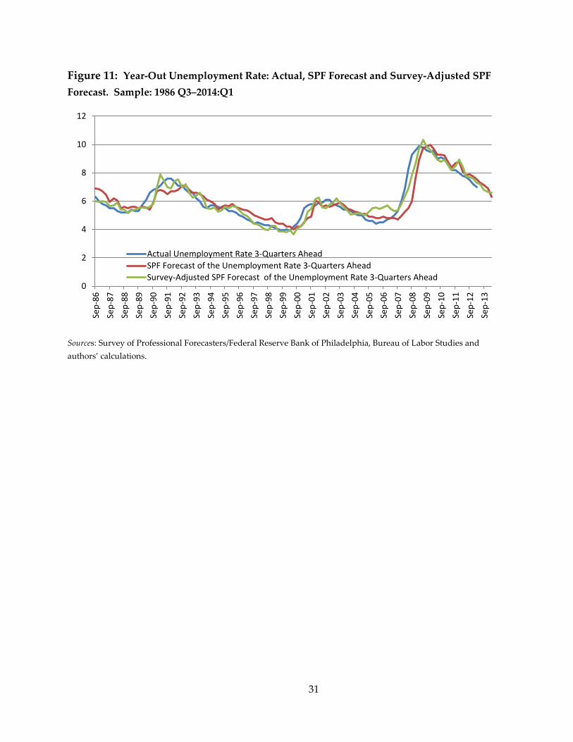
Figure 11: Year-Out Unemployment Rate: Actual, SPF Forecast and Survey-Adjusted SPF Forecast. Sample: 1986 Q3–2014:Q1
Sources: Survey of Professional Forecasters/Federal Reserve Bank of Philadelphia, Bureau of Labor Studies and authors’ calculations.
0
2
4
6
8
10
12
Sep-
86Se
p-87
Sep-
88Se
p-89
Sep-
90Se
p-91
Sep-
92Se
p-93
Sep-
94Se
p-95
Sep-
96Se
p-97
Sep-
98Se
p-99
Sep-
00Se
p-01
Sep-
02Se
p-03
Sep-
04Se
p-05
Sep-
06Se
p-07
Sep-
08Se
p-09
Sep-
10Se
p-11
Sep-
12Se
p-13
Actual Unemployment Rate 3-Quarters AheadSPF Forecast of the Unemployment Rate 3-Quarters AheadSurvey-Adjusted SPF Forecast of the Unemployment Rate 3-Quarters Ahead
31
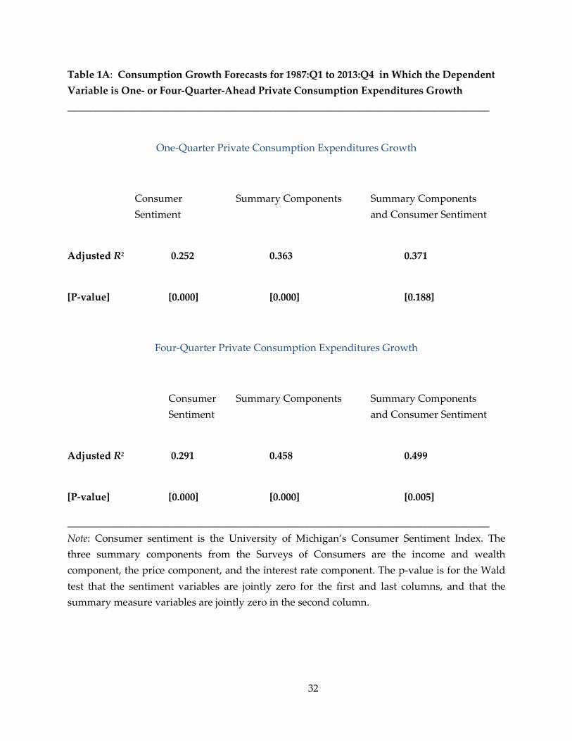
Table 1A: Consumption Growth Forecasts for 1987:Q1 to 2013:Q4 in Which the Dependent Variable is One- or Four-Quarter-Ahead Private Consumption Expenditures Growth __________________________________________________________________________________
One-Quarter Private Consumption Expenditures Growth
Consumer Summary Components Summary Components Sentiment and Consumer Sentiment
Adjusted R2 0.252 0.363 0.371
[P-value] [0.000] [0.000] [0.188]
Four-Quarter Private Consumption Expenditures Growth
Consumer Summary Components Summary Components Sentiment and Consumer Sentiment
Adjusted R2 0.291 0.458 0.499
[P-value] [0.000] [0.000] [0.005]
__________________________________________________________________________________ Note: Consumer sentiment is the University of Michigan’s Consumer Sentiment Index. The three summary components from the Surveys of Consumers are the income and wealth component, the price component, and the interest rate component. The p-value is for the Wald test that the sentiment variables are jointly zero for the first and last columns, and that the summary measure variables are jointly zero in the second column.
32
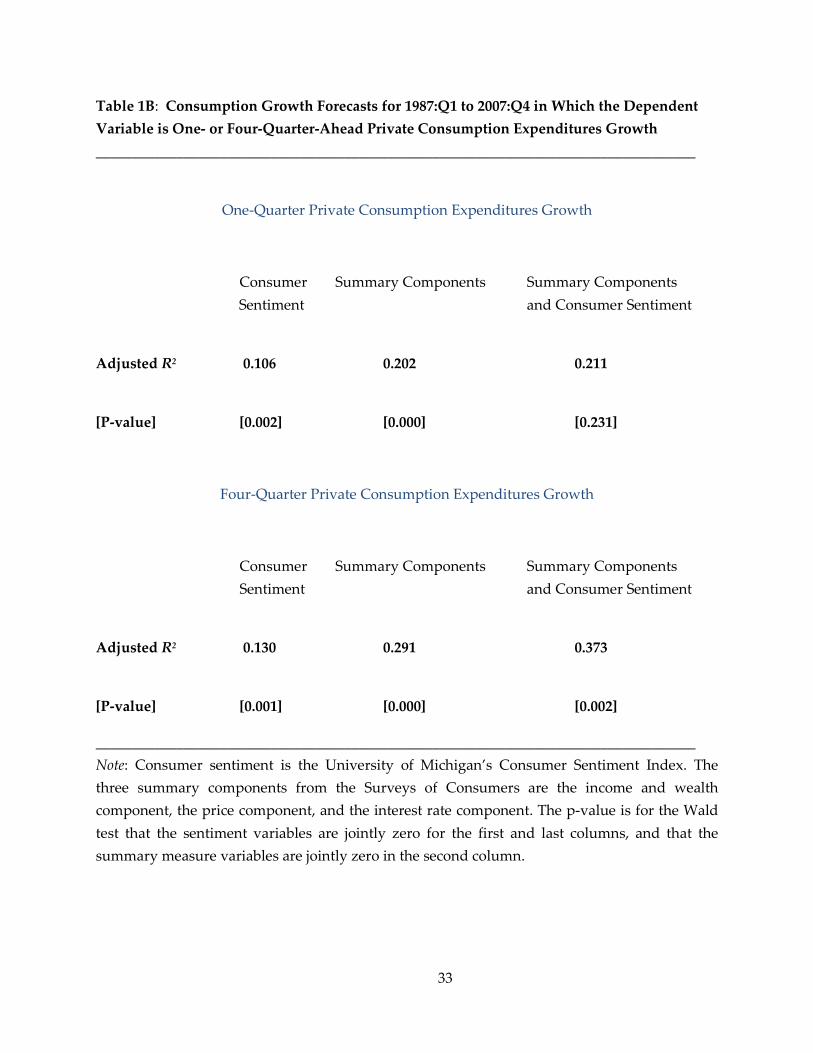
Table 1B: Consumption Growth Forecasts for 1987:Q1 to 2007:Q4 in Which the Dependent Variable is One- or Four-Quarter-Ahead Private Consumption Expenditures Growth __________________________________________________________________________________
One-Quarter Private Consumption Expenditures Growth
Consumer Summary Components Summary Components Sentiment and Consumer Sentiment
Adjusted R2 0.106 0.202 0.211
[P-value] [0.002] [0.000] [0.231]
Four-Quarter Private Consumption Expenditures Growth
Consumer Summary Components Summary Components Sentiment and Consumer Sentiment
Adjusted R2 0.130 0.291 0.373
[P-value] [0.001] [0.000] [0.002]
__________________________________________________________________________________ Note: Consumer sentiment is the University of Michigan’s Consumer Sentiment Index. The three summary components from the Surveys of Consumers are the income and wealth component, the price component, and the interest rate component. The p-value is for the Wald test that the sentiment variables are jointly zero for the first and last columns, and that the summary measure variables are jointly zero in the second column.
33
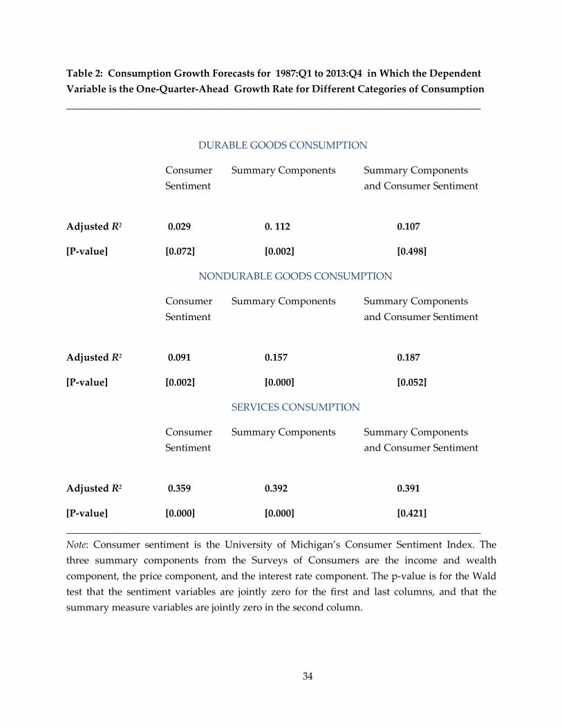
Table 2: Consumption Growth Forecasts for 1987:Q1 to 2013:Q4 in Which the Dependent Variable is the One-Quarter-Ahead Growth Rate for Different Categories of Consumption __________________________________________________________________________________
DURABLE GOODS CONSUMPTION
Consumer Summary Components Summary Components Sentiment and Consumer Sentiment
Adjusted R2 0.029 0. 112 0.107
[P-value] [0.072] [0.002] [0.498]
NONDURABLE GOODS CONSUMPTION
Consumer Summary Components Summary Components Sentiment and Consumer Sentiment
Adjusted R2 0.091 0.157 0.187
[P-value] [0.002] [0.000] [0.052]
SERVICES CONSUMPTION
Consumer Summary Components Summary Components Sentiment and Consumer Sentiment
Adjusted R2 0.359 0.392 0.391
[P-value] [0.000] [0.000] [0.421] __________________________________________________________________________________ Note: Consumer sentiment is the University of Michigan’s Consumer Sentiment Index. The three summary components from the Surveys of Consumers are the income and wealth component, the price component, and the interest rate component. The p-value is for the Wald test that the sentiment variables are jointly zero for the first and last columns, and that the summary measure variables are jointly zero in the second column.
34
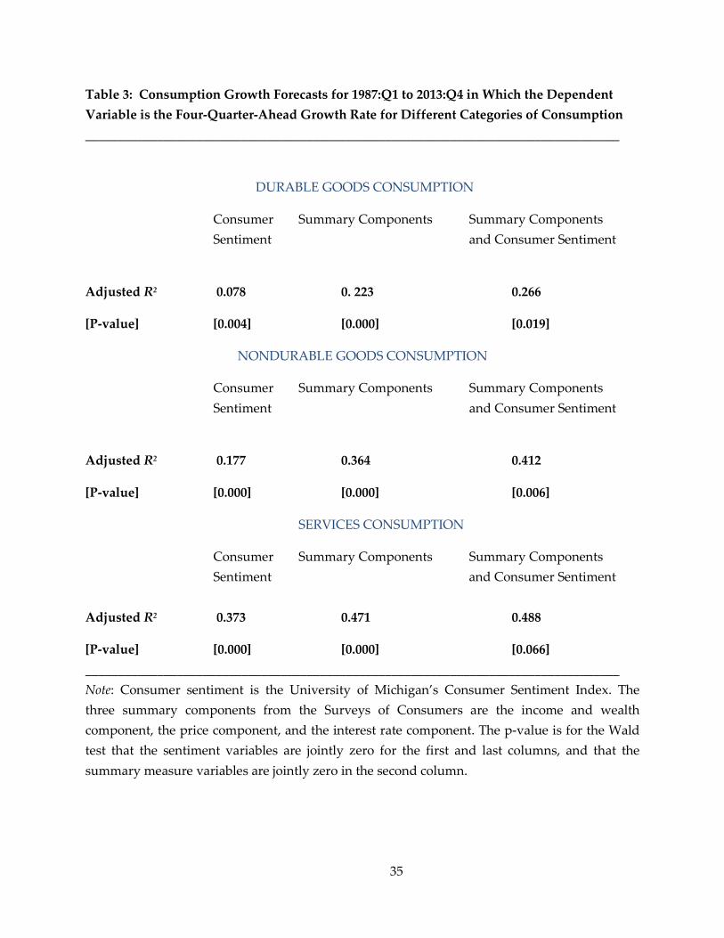
Table 3: Consumption Growth Forecasts for 1987:Q1 to 2013:Q4 in Which the Dependent Variable is the Four-Quarter-Ahead Growth Rate for Different Categories of Consumption __________________________________________________________________________________
DURABLE GOODS CONSUMPTION
Consumer Summary Components Summary Components Sentiment and Consumer Sentiment
Adjusted R2 0.078 0. 223 0.266
[P-value] [0.004] [0.000] [0.019]
NONDURABLE GOODS CONSUMPTION
Consumer Summary Components Summary Components Sentiment and Consumer Sentiment
Adjusted R2 0.177 0.364 0.412
[P-value] [0.000] [0.000] [0.006]
SERVICES CONSUMPTION
Consumer Summary Components Summary Components Sentiment and Consumer Sentiment Adjusted R2 0.373 0.471 0.488
[P-value] [0.000] [0.000] [0.066] __________________________________________________________________________________ Note: Consumer sentiment is the University of Michigan’s Consumer Sentiment Index. The three summary components from the Surveys of Consumers are the income and wealth component, the price component, and the interest rate component. The p-value is for the Wald test that the sentiment variables are jointly zero for the first and last columns, and that the summary measure variables are jointly zero in the second column.
35
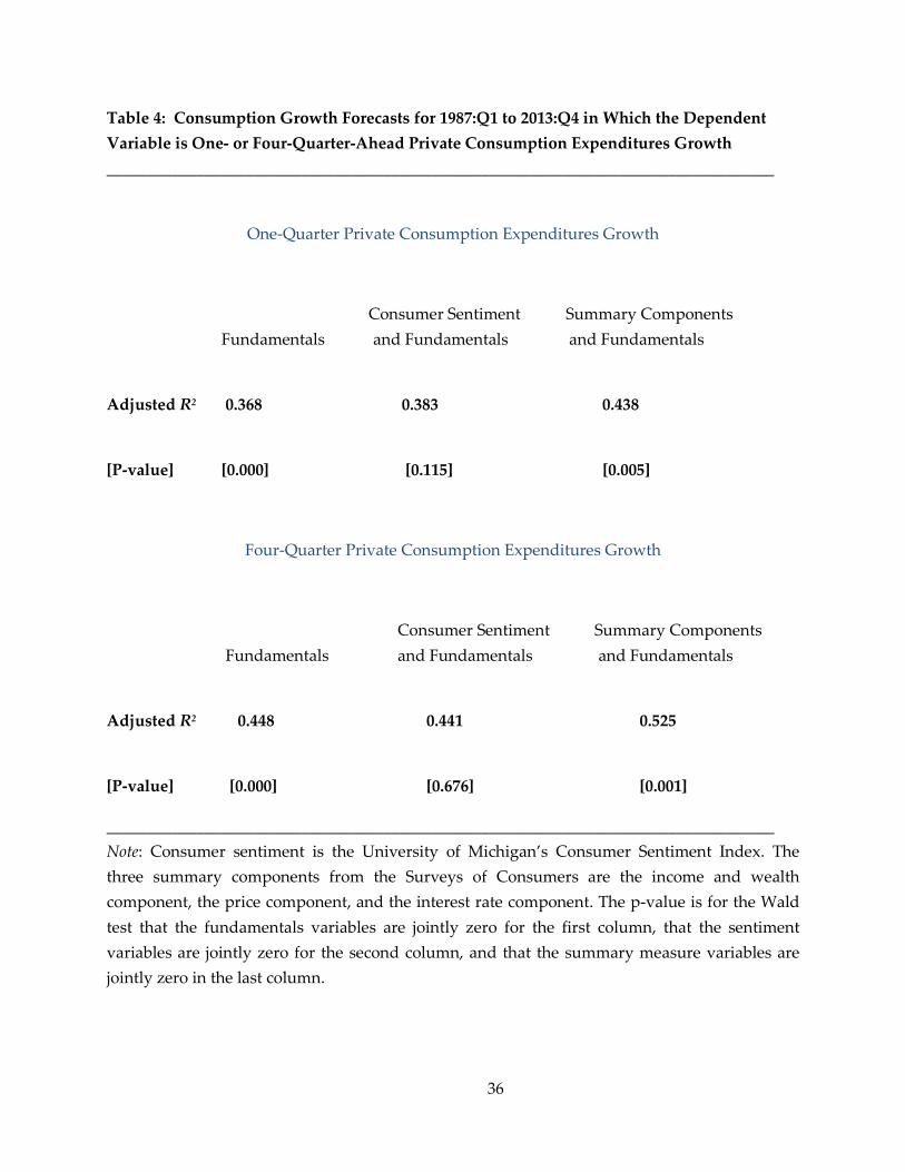
Table 4: Consumption Growth Forecasts for 1987:Q1 to 2013:Q4 in Which the Dependent Variable is One- or Four-Quarter-Ahead Private Consumption Expenditures Growth __________________________________________________________________________________
One-Quarter Private Consumption Expenditures Growth
Consumer Sentiment Summary Components Fundamentals and Fundamentals and Fundamentals
Adjusted R2 0.368 0.383 0.438
[P-value] [0.000] [0.115] [0.005]
Four-Quarter Private Consumption Expenditures Growth
Consumer Sentiment Summary Components Fundamentals and Fundamentals and Fundamentals
Adjusted R2 0.448 0.441 0.525
[P-value] [0.000] [0.676] [0.001]
__________________________________________________________________________________ Note: Consumer sentiment is the University of Michigan’s Consumer Sentiment Index. The three summary components from the Surveys of Consumers are the income and wealth component, the price component, and the interest rate component. The p-value is for the Wald test that the fundamentals variables are jointly zero for the first column, that the sentiment variables are jointly zero for the second column, and that the summary measure variables are jointly zero in the last column.
36
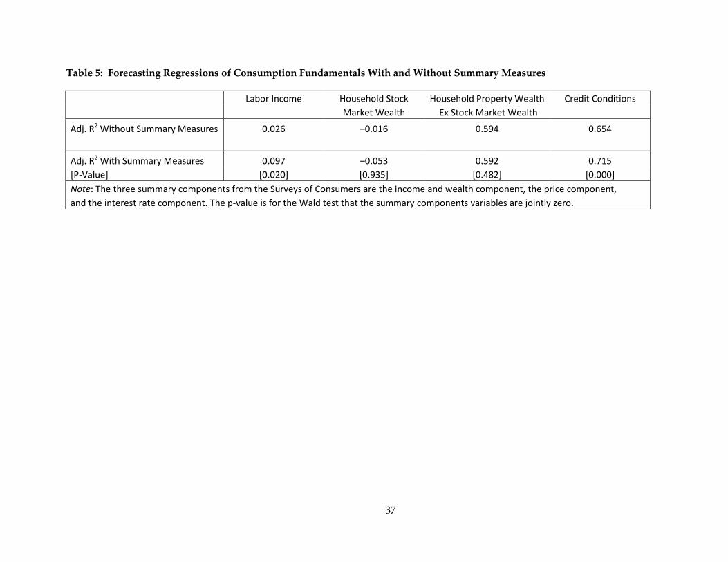
Table 5: Forecasting Regressions of Consumption Fundamentals With and Without Summary Measures
Labor Income Household Stock Household Property Wealth Credit Conditions Market Wealth Ex Stock Market Wealth
Adj. R2 Without Summary Measures 0.026 –0.016 0.594 0.654
Adj. R2 With Summary Measures 0.097 –0.053 0.592 0.715 [P-Value] [0.020] [0.935] [0.482] [0.000] Note: The three summary components from the Surveys of Consumers are the income and wealth component, the price component, and the interest rate component. The p-value is for the Wald test that the summary components variables are jointly zero.
37
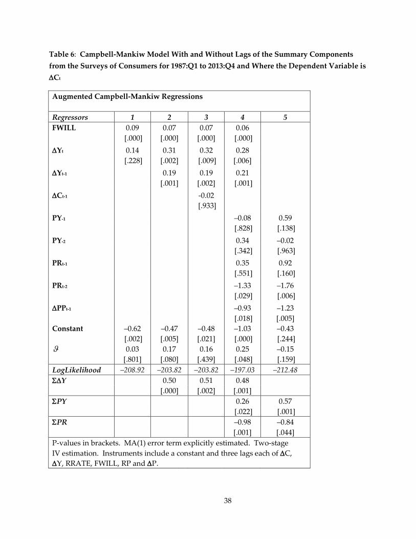
Table 6: Campbell-Mankiw Model With and Without Lags of the Summary Components from the Surveys of Consumers for 1987:Q1 to 2013:Q4 and Where the Dependent Variable is ∆Ct
Augmented Campbell-Mankiw Regressions Regressors 1 2 3 4 5 FWILL 0.09 0.07 0.07 0.06 [.000] [.000] [.000] [.000] ∆Yt 0.14 0.31 0.32 0.28 [.228] [.002] [.009] [.006] ∆Yt-1 0.19 0.19 0.21 [.001] [.002] [.001] ∆Ct-1 -0.02 [.933] PY-1 –0.08 0.59 [.828] [.138] PY-2 0.34 –0.02 [.342] [.963] PRt-1 0.35 0.92 [.551] [.160] PRt-2 –1.33 –1.76 [.029] [.006] ∆PPt-1 –0.93 –1.23 [.018] [.005] Constant –0.62 –0.47 –0.48 –1.03 –0.43 [.002] [.005] [.021] [.000] [.244] ϑ 0.03 0.17 0.16 0.25 –0.15 [.801] [.080] [.439] [.048] [.159] LogLikelihood –208.92 –203.82 –203.82 –197.03 –212.48 Σ∆Y 0.50 0.51 0.48 [.000] [.002] [.001] ΣPY 0.26 0.57 [.022] [.001] ΣPR –0.98 –0.84 [.001] [.044] P-values in brackets. MA(1) error term explicitly estimated. Two-stage IV estimation. Instruments include a constant and three lags each of ∆C, ∆Y, RRATE, FWILL, RP and ∆P.
38
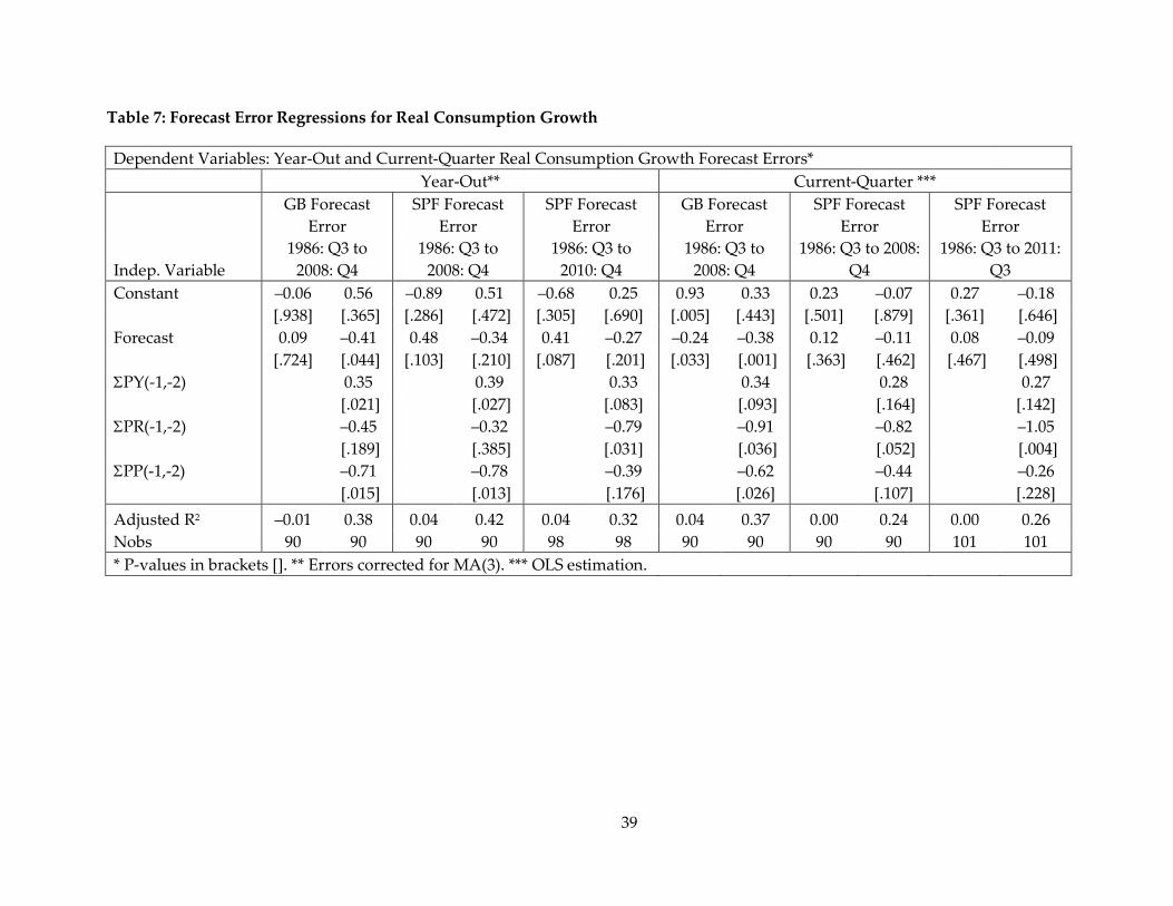
Table 7: Forecast Error Regressions for Real Consumption Growth
Dependent Variables: Year-Out and Current-Quarter Real Consumption Growth Forecast Errors* Year-Out** Current-Quarter ***
GB Forecast
Error SPF Forecast
Error SPF Forecast
Error GB Forecast
Error SPF Forecast
Error SPF Forecast
Error
Indep. Variable 1986: Q3 to
2008: Q4 1986: Q3 to
2008: Q4 1986: Q3 to
2010: Q4 1986: Q3 to
2008: Q4 1986: Q3 to 2008:
Q4 1986: Q3 to 2011:
Q3 Constant –0.06 0.56 –0.89 0.51 –0.68 0.25 0.93 0.33 0.23 –0.07 0.27 –0.18 [.938] [.365] [.286] [.472] [.305] [.690] [.005] [.443] [.501] [.879] [.361] [.646] Forecast 0.09 –0.41 0.48 –0.34 0.41 –0.27 –0.24 –0.38 0.12 –0.11 0.08 –0.09 [.724] [.044] [.103] [.210] [.087] [.201] [.033] [.001] [.363] [.462] [.467] [.498] ΣPY(-1,-2) 0.35 0.39 0.33 0.34 0.28 0.27
[.021] [.027] [.083] [.093] [.164] [.142]
ΣPR(-1,-2) –0.45 –0.32 –0.79 –0.91 –0.82 –1.05 [.189] [.385] [.031] [.036] [.052] [.004] ΣPP(-1,-2) –0.71 –0.78 –0.39 –0.62 –0.44 –0.26 [.015] [.013] [.176] [.026] [.107] [.228] Adjusted R2 –0.01 0.38 0.04 0.42 0.04 0.32 0.04 0.37 0.00 0.24 0.00 0.26 Nobs 90 90 90 90 98 98 90 90 90 90 101 101 * P-values in brackets []. ** Errors corrected for MA(3). *** OLS estimation.
39
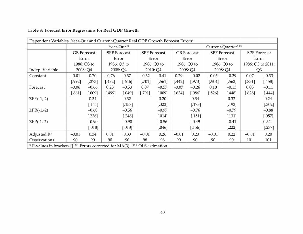
Table 8: Forecast Error Regressions for Real GDP Growth
Dependent Variables: Year-Out and Current-Quarter Real GDP Growth Forecast Errors* Year-Out** Current-Quarter***
GB Forecast
Error SPF Forecast
Error SPF Forecast
Error GB Forecast
Error SPF Forecast
Error SPF Forecast
Error
Indep. Variable 1986: Q3 to
2008: Q4 1986: Q3 to
2008: Q4 1986: Q3 to
2010: Q4 1986: Q3 to
2008: Q4 1986: Q3 to
2008: Q4 1986: Q3 to 2011:
Q3 Constant –0.01 0.70 –0.76 0.37 –0.32 0.41 0.29 –0.02 -0.05 –0.29 0.07 –0.33 [.992] [.373] [.472] [.646] [.701] [.561] [.442] [.973] [.904] [.562] [.831] [.458] Forecast –0.06 –0.66 0.23 –0.53 0.07 –0.57 -0.07 –0.26 0.10 –0.13 0.03 –0.11 [.861] [.009] [.499] [.049] [.791] [.009] [.634] [.086] [.526] [.448] [.828] [.444] ΣPY(-1,-2) 0.34 0.32 0.20 0.34 0.32 0.24
[.141] [.158] [.323] [.173] [.193] [.302]
ΣPR(-1,-2) –0.60 –0.56 –0.97 –0.76 –0.79 –0.88 [.236] [.248] [.014] [.151] [.131] [.057] ΣPP(-1,-2) –0.90 –0.90 –0.56 –0.49 –0.41 –0.32 [.018] [.013] [.046] [.156] [.222] [.237] Adjusted R2 –0.01 0.34 0.01 0.33 –0.01 0.26 –0.01 0.23 –0.01 0.22 –0.01 0.20 Observations 90 90 90 90 98 98 90 90 90 90 101 101 * P-values in brackets []. ** Errors corrected for MA(3). *** OLS estimation.
40
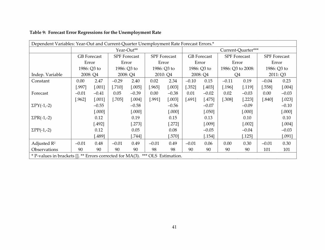
Table 9: Forecast Error Regressions for the Unemployment Rate
Dependent Variables: Year-Out and Current-Quarter Unemployment Rate Forecast Errors.* Year-Out** Current-Quarter***
GB Forecast
Error SPF Forecast
Error SPF Forecast
Error GB Forecast
Error SPF Forecast
Error SPF Forecast
Error
Indep. Variable 1986: Q3 to
2008: Q4 1986: Q3 to
2008: Q4 1986: Q3 to
2010: Q4 1986: Q3 to
2008: Q4 1986: Q3 to 2008:
Q4 1986: Q3 to 2011: Q3
Constant 0.00 2.47 –0.29 2.40 0.02 2.34 –0.10 0.15 –0.11 0.19 –0.04 0.23 [.997] [.001] [.710] [.005] [.965] [.003] [.352] [.403] [.196] [.119] [.558] [.004] Forecast –0.01 –0.41 0.05 –0.39 0.00 –0.38 0.01 –0.02 0.02 –0.03 0.00 –0.03 [.962] [.001] [.705] [.004] [.991] [.003] [.691] [.475] [.308] [.223] [.840] [.023] ΣPY(-1,-2) –0.55 –0.58 –0.56 –0.07 –0.09 –0.10
[.000] [.000] [.000] [.050] [.000] [.000]
ΣPR(-1,-2) 0.12 0.19 0.15 0.13 0.10 0.10 [.492] [.273] [.272] [.009] [.002] [.004] ΣPP(-1,-2) 0.12 0.05 0.08 –0.05 –0.04 –0.03 [.489] [.744] [.570] [.154] [.125] [.091] Adjusted R2 –0.01 0.48 –0.01 0.49 –0.01 0.49 –0.01 0.06 0.00 0.30 –0.01 0.30 Observations 90 90 90 90 98 98 90 90 90 90 101 101 * P-values in brackets []. ** Errors corrected for MA(3). *** OLS Estimation.
41
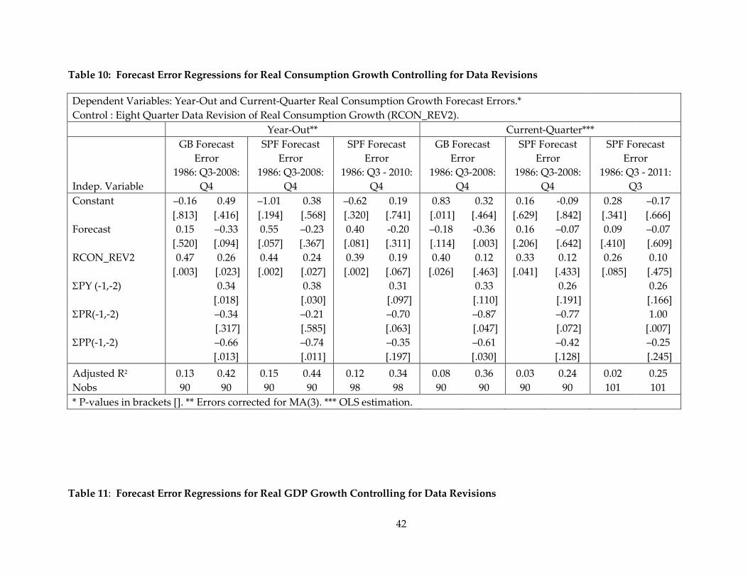
Table 10: Forecast Error Regressions for Real Consumption Growth Controlling for Data Revisions
Dependent Variables: Year-Out and Current-Quarter Real Consumption Growth Forecast Errors.* Control : Eight Quarter Data Revision of Real Consumption Growth (RCON_REV2). Year-Out** Current-Quarter***
GB Forecast
Error SPF Forecast
Error SPF Forecast
Error GB Forecast
Error SPF Forecast
Error SPF Forecast
Error
Indep. Variable 1986: Q3-2008:
Q4 1986: Q3-2008:
Q4 1986: Q3 - 2010:
Q4 1986: Q3-2008:
Q4 1986: Q3-2008:
Q4 1986: Q3 - 2011:
Q3 Constant –0.16 0.49 –1.01 0.38 –0.62 0.19 0.83 0.32 0.16 -0.09 0.28 –0.17 [.813] [.416] [.194] [.568] [.320] [.741] [.011] [.464] [.629] [.842] [.341] [.666] Forecast 0.15 –0.33 0.55 –0.23 0.40 -0.20 –0.18 -0.36 0.16 –0.07 0.09 –0.07 [.520] [.094] [.057] [.367] [.081] [.311] [.114] [.003] [.206] [.642] [.410] [.609] RCON_REV2 0.47 0.26 0.44 0.24 0.39 0.19 0.40 0.12 0.33 0.12 0.26 0.10 [.003] [.023] [.002] [.027] [.002] [.067] [.026] [.463] [.041] [.433] [.085] [.475] ΣPY (-1,-2) 0.34 0.38 0.31 0.33 0.26 0.26
[.018] [.030] [.097] [.110] [.191] [.166]
ΣPR(-1,-2) –0.34 –0.21 –0.70 –0.87 –0.77 1.00 [.317] [.585] [.063] [.047] [.072] [.007] ΣPP(-1,-2) –0.66 –0.74 –0.35 –0.61 –0.42 –0.25 [.013] [.011] [.197] [.030] [.128] [.245] Adjusted R2 0.13 0.42 0.15 0.44 0.12 0.34 0.08 0.36 0.03 0.24 0.02 0.25 Nobs 90 90 90 90 98 98 90 90 90 90 101 101 * P-values in brackets []. ** Errors corrected for MA(3). *** OLS estimation.
Table 11: Forecast Error Regressions for Real GDP Growth Controlling for Data Revisions
42
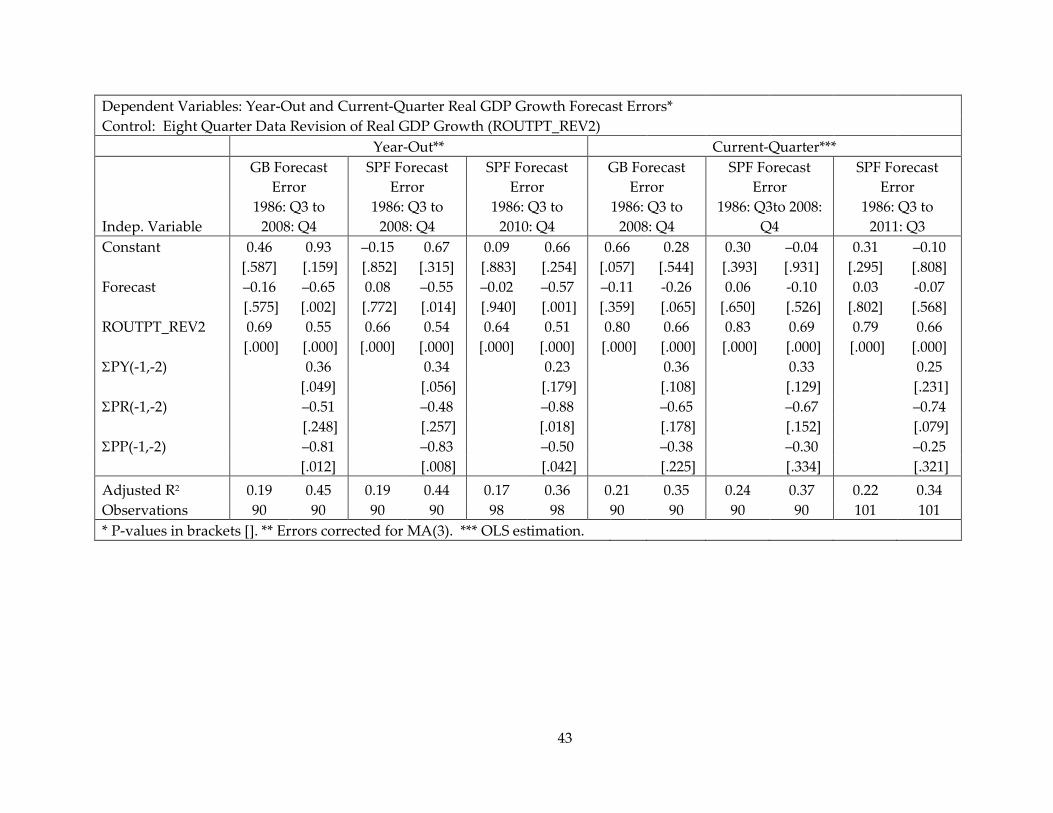
Dependent Variables: Year-Out and Current-Quarter Real GDP Growth Forecast Errors* Control: Eight Quarter Data Revision of Real GDP Growth (ROUTPT_REV2) Year-Out** Current-Quarter***
GB Forecast
Error SPF Forecast
Error SPF Forecast
Error GB Forecast
Error SPF Forecast
Error SPF Forecast
Error
Indep. Variable 1986: Q3 to
2008: Q4 1986: Q3 to
2008: Q4 1986: Q3 to
2010: Q4 1986: Q3 to
2008: Q4 1986: Q3to 2008:
Q4 1986: Q3 to
2011: Q3 Constant 0.46 0.93 –0.15 0.67 0.09 0.66 0.66 0.28 0.30 –0.04 0.31 –0.10 [.587] [.159] [.852] [.315] [.883] [.254] [.057] [.544] [.393] [.931] [.295] [.808] Forecast –0.16 –0.65 0.08 –0.55 –0.02 –0.57 –0.11 -0.26 0.06 -0.10 0.03 -0.07 [.575] [.002] [.772] [.014] [.940] [.001] [.359] [.065] [.650] [.526] [.802] [.568] ROUTPT_REV2 0.69 0.55 0.66 0.54 0.64 0.51 0.80 0.66 0.83 0.69 0.79 0.66 [.000] [.000] [.000] [.000] [.000] [.000] [.000] [.000] [.000] [.000] [.000] [.000] ΣPY(-1,-2) 0.36 0.34 0.23 0.36 0.33 0.25
[.049] [.056] [.179] [.108] [.129] [.231]
ΣPR(-1,-2) –0.51 –0.48 –0.88 –0.65 –0.67 –0.74 [.248] [.257] [.018] [.178] [.152] [.079] ΣPP(-1,-2) –0.81 –0.83 –0.50 –0.38 –0.30 –0.25 [.012] [.008] [.042] [.225] [.334] [.321] Adjusted R2 0.19 0.45 0.19 0.44 0.17 0.36 0.21 0.35 0.24 0.37 0.22 0.34 Observations 90 90 90 90 98 98 90 90 90 90 101 101 * P-values in brackets []. ** Errors corrected for MA(3). *** OLS estimation.
43
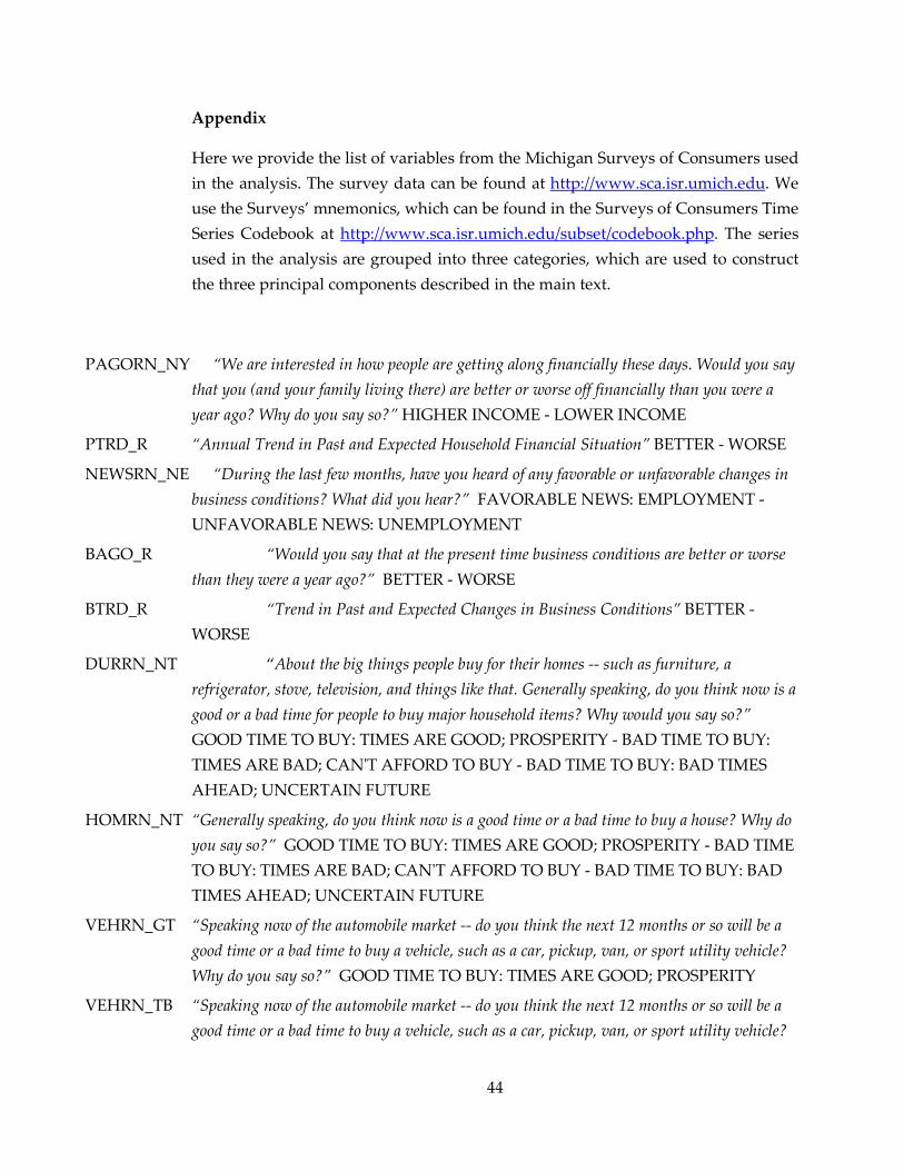
Appendix
Here we provide the list of variables from the Michigan Surveys of Consumers used in the analysis. The survey data can be found at http://www.sca.isr.umich.edu. We use the Surveys’ mnemonics, which can be found in the Surveys of Consumers Time Series Codebook at http://www.sca.isr.umich.edu/subset/codebook.php. The series used in the analysis are grouped into three categories, which are used to construct the three principal components described in the main text.
PAGORN_NY “We are interested in how people are getting along financially these days. Would you say that you (and your family living there) are better or worse off financially than you were a year ago? Why do you say so?” HIGHER INCOME - LOWER INCOME
PTRD_R “Annual Trend in Past and Expected Household Financial Situation” BETTER - WORSE
NEWSRN_NE “During the last few months, have you heard of any favorable or unfavorable changes in business conditions? What did you hear?” FAVORABLE NEWS: EMPLOYMENT - UNFAVORABLE NEWS: UNEMPLOYMENT
BAGO_R “Would you say that at the present time business conditions are better or worse than they were a year ago?” BETTER - WORSE
BTRD_R “Trend in Past and Expected Changes in Business Conditions” BETTER - WORSE
DURRN_NT “About the big things people buy for their homes -- such as furniture, a refrigerator, stove, television, and things like that. Generally speaking, do you think now is a good or a bad time for people to buy major household items? Why would you say so?” GOOD TIME TO BUY: TIMES ARE GOOD; PROSPERITY - BAD TIME TO BUY: TIMES ARE BAD; CAN'T AFFORD TO BUY - BAD TIME TO BUY: BAD TIMES AHEAD; UNCERTAIN FUTURE
HOMRN_NT “Generally speaking, do you think now is a good time or a bad time to buy a house? Why do you say so?” GOOD TIME TO BUY: TIMES ARE GOOD; PROSPERITY - BAD TIME TO BUY: TIMES ARE BAD; CAN'T AFFORD TO BUY - BAD TIME TO BUY: BAD TIMES AHEAD; UNCERTAIN FUTURE
VEHRN_GT “Speaking now of the automobile market -- do you think the next 12 months or so will be a good time or a bad time to buy a vehicle, such as a car, pickup, van, or sport utility vehicle? Why do you say so?” GOOD TIME TO BUY: TIMES ARE GOOD; PROSPERITY
VEHRN_TB “Speaking now of the automobile market -- do you think the next 12 months or so will be a good time or a bad time to buy a vehicle, such as a car, pickup, van, or sport utility vehicle?
44

Why do you say so?” BAD TIME TO BUY: TIMES ARE BAD; CAN’T AFFORD TO BUY
VEHRN_FB “Speaking now of the automobile market -- do you think the next 12 months or so will be a good time or a bad time to buy a vehicle, such as a car, pickup, van, or sport utility vehicle? Why do you say so?” BAD TIME TO BUY: BAD TIMES AHEAD, UNCERTAIN FUTURE
NEWSRN_F_DEM “During the last few months, have you heard of any favorable or unfavorable changes in business conditions? What did you hear?” FAVORABLE NEWS: HIGHER CONSUMER DEMAND
NEWSRN_U_DEM “During the last few months, have you heard of any favorable or unfavorable changes in business conditions? What did you hear?” UNFAVORABLE NEWS: LOWER CONSUMER DEMAND
PEXP_R “Now looking ahead -- do you think that a year from now you (and your family living there) will be better off financially, worse off, or just about the same as now?” BETTER - WORSE
INEX_R “During the next 12 months, do you expect your (family) income to be higher or lower than during the past year?” RELATIVE SCORE
RINC_R “During the next year or two, do you expect that your (family) income will go up more than prices will go up, about the same, or less than prices will go up?” MORE - LESS
BEXP_R “And how about a year from now, do you expect that in the country as a whole business conditions will be better, or worse than they are at present, or just about the same?” BETTER - WORSE
BUS12_R “Now turning to business conditions in the country as a whole -- do you think that during the next 12 months we'll have good times financially, or bad times, or what?” GOOD - BAD
BUS5_R “Looking ahead, which would you say is more likely -- that in the country as a whole we'll have continuous good times during the next 5 years or so, or that we will have periods of widespread unemployment or depression, or what?” GOOD - BAD
UMEX_R “How about people out of work during the coming 12 months -- do you think that there will be more unemployment than now, about the same, or less?” LESS - MORE
PAGORN_NAD “We are interested in how people are getting along financially these days. Would you say that you (and your family living there) are better or worse off financially than you were a year ago? Why do you say so?” HIGHER ASSETS + LOWER DEBTS - LOWER ASSETS - HIGHER DEBTS
45

NEWSRN_F_STK “During the last few months, have you heard of any favorable or unfavorable changes in business conditions? What did you hear?” FAVORABLE NEWS: STOCK MARKET
NEWSRN_U_STK “During the last few months, have you heard of any favorable or unfavorable changes in business conditions? What did you hear?” UNFAVORABLE NEWS: STOCK MARKET
HOMRN_NP “Generally speaking, do you think now is a good time or a bad time to buy a house? Why do you say so?” GOOD TIME TO BUY: PRICES ARE LOW; GOOD BUYS AVAILABLE - BAD TIME TO BUY: PRICES HIGH
HOMRN_NI “Generally speaking, do you think now is a good time or a bad time to buy a house? Why do you say so?” GOOD TIME TO BUY: GOOD INVESTMENT - BAD TIME TO BUY: BAD INVESTMENT
HOMRN_BIAP “Generally speaking, do you think now is a good time or a bad time to buy a house? Why do you say so?” GOOD TIME TO BUY: PRICES WON’T COME DOWN; ARE GOING HIGHER
PAGORN_HP “We are interested in how people are getting along financially these days. Would you say that you (and your family living there) are better or worse off financially than you were a year ago? Why do you say so?” HIGHER PRICES
NEWSRN_NP “During the last few months, have you heard of any favorable or unfavorable changes in business conditions? What did you hear?” FAVORABLE NEWS: LOWER PRICES - UNFAVORABLE NEWS: HIGHER PRICES
DURRN_NP “About the big things people buy for their homes -- such as furniture, a refrigerator, stove, television, and things like that. Generally speaking, do you think now is a good or a bad time for people to buy major household items? Why would you say so?” GOOD TIME TO BUY: PRICES ARE LOW; GOOD BUYS AVAILABLE - BAD TIME TO BUY: PRICES ARE HIGH
VEHRN_NP “Speaking now of the automobile market -- do you think the next 12 months or so will be a good time or a bad time to buy a vehicle, such as a car, pickup, van, or sport utility vehicle? Why do you say so?” GOOD TIME TO BUY: PRICES ARE LOW; GOOD BUYS AVAILABLE - BAD TIME TO BUY: PRICES ARE HIGH
PX1_MED “During the next 12 months, do you think that prices in general will go up, or go down, or stay where they are now? By what percent do you expect prices to go up, on the average, during the next 12 months?” MEDIAN
46

DURRN_BIAP “About the big things people buy for their homes -- such as furniture, a refrigerator, stove, television, and things like that. Generally speaking, do you think now is a good or a bad time for people to buy major household items? Why would you say so?” GOOD TIME TO BUY: PRICES WON'T COME DOWN; ARE GOING HIGHER
VEHRN_BIAP “Speaking now of the automobile market -- do you think the next 12 months or so will be a good time or a bad time to buy a vehicle, such as a car, pickup, van, or sport utility vehicle? Why do you say so?” GOOD TIME TO BUY: PRICES WON'T COME DOWN; ARE GOING HIGHER
VEHRN_GAS “Speaking now of the automobile market -- do you think the next 12 months or so will be a good time or a bad time to buy a vehicle, such as a car, pickup, van, or sport utility vehicle? Why do you say so?” BAD TIME TO BUY: PRICE OF GAS
NEWSRN_F_CRED “During the last few months, have you heard of any favorable or unfavorable changes in business conditions? What did you hear?” FAVORABLE NEWS: EASIER CREDIT
NEWSRN_U_CRED “During the last few months, have you heard of any favorable or unfavorable changes in business conditions? What did you hear?” UNFAVORABLE NEWS: TIGHTER CREDIT
DURRN_NR “About the big things people buy for their homes -- such as furniture, a refrigerator, stove, television, and things like that. Generally speaking, do you think now is a good or a bad time for people to buy major household items? Why would you say so?” GOOD TIME TO BUY: INTEREST RATES ARE LOW - BAD TIME TO BUY: INTEREST RATES ARE HIGH; CREDIT IS TIGHT
VEHRN_NR “Speaking now of the automobile market -- do you think the next 12 months or so will be a good time or a bad time to buy a vehicle, such as a car, pickup, van, or sport utility vehicle? Why do you say so?” GOOD TIME TO BUY: INTEREST RATES ARE LOW - BAD TIME TO BUY: INTEREST RATES ARE HIGH; CREDIT IS TIGHT
HOMRN_NR “Generally speaking, do you think now is a good time or a bad time to buy a house? Why do you say so?” GOOD TIME TO BUY: INTEREST RATES ARE LOW - BAD TIME TO BUY: INTEREST RATES ARE HIGH; CREDIT IS TIGHT
RATEX_R “No one can say for sure, but what do you think will happen to interest rates for borrowing money during the next 12 months -- will they go up, stay the same, or go down?” DOWN - UP
DURRN_BIAR “About the big things people buy for their homes -- such as furniture, a refrigerator, stove, television, and things like that. Generally speaking, do you think now is a good or a
47

bad time for people to buy major household items? Why would you say so?” GOOD TIME TO BUY: BORROW IN ADVANCE OF RISING INTEREST RATES
VEHRN_BIAR “Speaking now of the automobile market -- do you think the next 12 months or so will be a good time or a bad time to buy a vehicle, such as a car, pickup, van, or sport utility vehicle? Why do you say so?” GOOD TIME TO BUY: BORROW IN ADVANCE OF RISING INTEREST RATES
HOMRN_BIAR “Generally speaking, do you think now is a good time or a bad time to buy a house? Why do you say so?” GOOD TIME TO BUY: BORROW IN ADVANCE OF RISING INTEREST RATES
48

49
Recommended