© Crown copyright 2004 Page 1
The
Forecasting Ocean Assimilation Model
System
Mike Bell 25 Sept 2004
© Crown copyright 2004 Page 2
Content
Summary of capability and formulation
Trouble shooting
Assessments
Adapting to changing world

© Crown copyright 2004 Page 3
Summary of capability and formulation
© Crown copyright 2004 Page 4
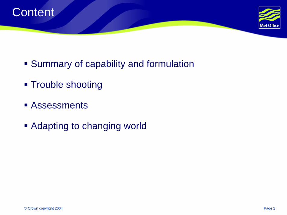
The Met Office’s Operational Ocean Products
SST analyses for NWP (global & regional); dailySurface waves (global & regional); twice dailyStorm surges to T+48: NW European shelf; twice dailyDeep ocean forecasts (T, S, u, v) to T+120; daily (FOAM)3D Shelf-seas (T, S, u, v) to T+48; daily (POLCOMS)Seasonal forecasts (coupled OIA); weekly (GloSea)SST and sea-ice analyses (HadISST); monthly
Operational characteristics: Routine service to existing (paying) usersTimeliness determined by user requirementsMonitoring and verification Dedicated operational staff
© Crown copyright 2004 Page 5
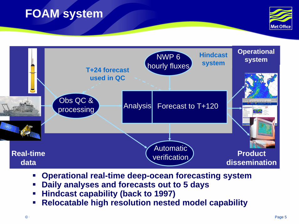
FOAM system
Operational real-time deep-ocean forecasting systemDaily analyses and forecasts out to 5 daysHindcast capability (back to 1997)Relocatable high resolution nested model capability
Real-time data
Obs QC & processing Analysis Forecast to T+120
NWP 6 hourly fluxes
Automatic verification
T+24 forecast used in QC
Product dissemination
Operational systemHindcast
system
© Crown copyright 2004 Page 6
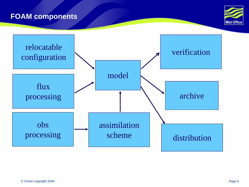
FOAM components
assimilationscheme
modelflux
processing
obsprocessing
archive
verification
distribution
relocatableconfiguration
© Crown copyright 2004 Page 7
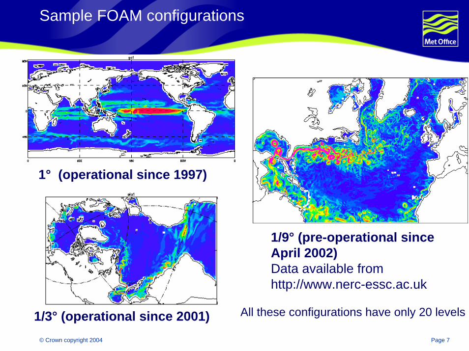
Sample FOAM configurations
1° (operational since 1997)
1/9° (pre-operational since April 2002) Data available from http://www.nerc-essc.ac.uk
1/3° (operational since 2001) All these configurations have only 20 levels
© Crown copyright 2004 Page 8
Relocatable Nested Configurations
Have used various bathymetries (Smith & Sandwell, GEBCO, DBDB2)
Use latitude-longitude grid (with rotated pole in limited area models to give uniform grid)
1-2-1 filter is applied twice to bathymetry to avoid forcing at grid-scale
Grid-scale channels are filled to prevent an instability (appears to be associated with B-grid)
Channels are adjusted using list by Thompson (1996)
Bathymetry in relaxation zone of nested models is “matched” to that of outer model
Flow relaxation scheme used for all prognostic variables with boundary rim of 4-8 points
© Crown copyright 2004 Page 9
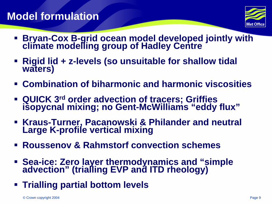
Model formulation
Bryan-Cox B-grid ocean model developed jointly with climate modelling group of Hadley CentreRigid lid + z-levels (so unsuitable for shallow tidal waters)Combination of biharmonic and harmonic viscositiesQUICK 3rd order advection of tracers; Griffiesisopycnal mixing; no Gent-McWilliams “eddy flux” Kraus-Turner, Pacanowski & Philander and neutral Large K-profile vertical mixingRoussenov & Rahmstorf convection schemes
Sea-ice: Zero layer thermodynamics and “simple advection” (trialling EVP and ITD rheology)Trialling partial bottom levels

© Crown copyright 2004 Page 10
Observations and surface fluxes
Temperature and salinity profile data at all depths
Surface temperature data; in situ and coarse grid (2.5o) AVHRR products
Altimeter data processed by CLS (Jason-1, Envisat, GFO) twice a week
Sea ice concentration fields from CMC (based on SSMI)
Surface fluxes from global NWP system: wind stress, wind mixing energy, heat fluxes (penetrating & non-), precipitation minus evaporation; weak Haney relaxation to climate T & S
Over sea-ice, both fluxes through ice and leads
River inflow (based on GRDC monthly climate; largest rivers modified; global only)
© Crown copyright 2004 Page 11
Formulation of Assimilation
Timely assimilation
Two component background error covariances
Revised FOAM assimilation scheme

© Crown copyright 2004 Page 12
Standard 4D-Variational Assimilation
Observation (y)
t
Initialcondition
(x)
Best fit
Assim time window
Adjust the initial condition until the sum of the squares of the normalised errors is minimised
1 1( ) ( ) [ ( ( ))] ( ) [ ( ( ))]T Tb bJ y h g O F y h g− −= − − + − + −x x B x x x x
© Crown copyright 2004 Page 13
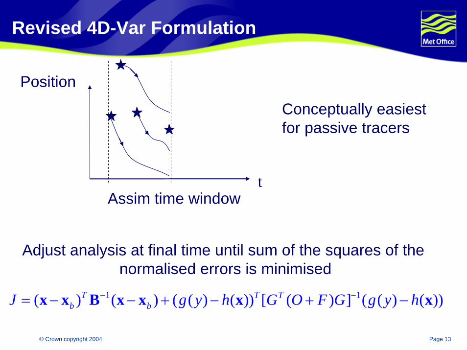
Revised 4D-Var Formulation
Position
Conceptually easiestfor passive tracers
tAssim time window
Adjust analysis at final time until sum of the squares of the normalised errors is minimised
1 1( ) ( ) ( ( ) ( )) [ ( ) ] ( ( ) ( ))T T Tb bJ g y h G O F G g y h− −= − − + − + −x x B x x x x
© Crown copyright 2004 Page 14
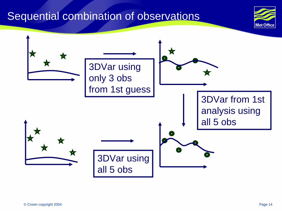
Sequential combination of observations
3DVar usingonly 3 obsfrom 1st guess
3DVar from 1st analysis usingall 5 obs
3DVar usingall 5 obs

© Crown copyright 2004 Page 15
Timely Variational Assimilation
Assimilate observations into the model fields as soon as they arrive
Keep track of where information from each observation has been received, evolving its location and increasing its estimated error with time
This method avoids having to calculate the evolution of the temperature (etc.) of each observation - which would be difficult to do accurately enough

© Crown copyright 2004 Page 16
Two component background error covariances
We assume the forecast errors arise from two distinct sources:errors in the internal model dynamics => “mesoscale” errorserrors in the atmospheric forcing & biases => “synoptic” scale errors
Assume separability of the error covariance for each component, i.e. horizontal and vertical correlations can be calculated separately:
Use collocated observation and model forecast values to estimate covariance values – bin together to have enough statistical information
Fit the sum of 2 SOAR functions to the (obs-f/c) covariance values to estimate the variance and horizontal correlation scales of the two forecast error components.
m s= +B B B
m m s sh v h v= +B B B B B
© Crown copyright 2004 Page 17
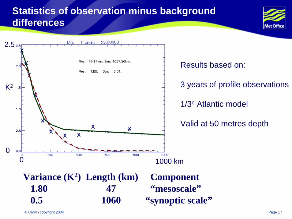
Statistics of observation minus background differences
x
x
x
x
xxx x x
x
Results based on:
3 years of profile observations
1/3o Atlantic model
Valid at 50 metres depth
1000 km
2.5
00
K2
Variance (K2) Length (km) Component 1.80 47 “mesoscale”0.5 1060 “synoptic scale”
© Crown copyright 2004 Page 18
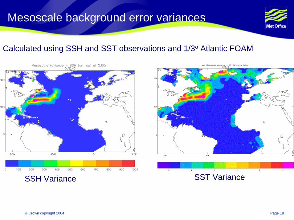
Mesoscale background error variances
Calculated using SSH and SST observations and 1/3o Atlantic FOAM
SST VarianceSSH Variance
© Crown copyright 2004 Page 19
Discussion of background error covariances
Spatial and temporal resolution of results is restricted by the number of observations
Difficult to extract information about vertical correlations
Observation errors assumed to be uncorrelated – not always true
Scales calculated are isotropic – could also calculate anisotropic scales using the same method
Some of these shortcomings could be addressed by using methods which estimate covariances using model fields, e.g. NMC method, although these methods don’t relate the model fields to the “truth”.
© Crown copyright 2004 Page 20
Outline of assimilation scheme
We perform one analysis each dayEach analysis consists of a number of iterations On each iteration observations are separated into groups which are easily related (thermal profiles, saline profiles, surface temperature, surface height)For each group of observations (e.g. the temperature profile data), increments are calculated first for the directly related model variables (e.g. the temperature fields) More detail on next slideThese increment fields are then used to calculate increments for less directly related model variables (e.g. the velocity fields using hydrostatic and geostrophic balance relationships)
The analysis increment fields are smoothly applied over the next24 hours

© Crown copyright 2004 Page 21
Details of univariate step
The analysis equation is ∆x= B HT (H B HT + R)-1 ∆y
We calculate the differences between each observation and the model (the observation increment vector ∆y)
B HTv is performed either as B (HTv) using a recursive filter or as (B HT) v by explicit calculations for each observation in its neighbourhood
Filtering performed for each component in 2 or 3 dimensions
A simple approximation is made to the matrix inverseMore efficient techniques could be implemented
We make increments to the observations so that the iterations converge to the 3DVar solution (Bratseth1986)
© Crown copyright 2004 Page 22
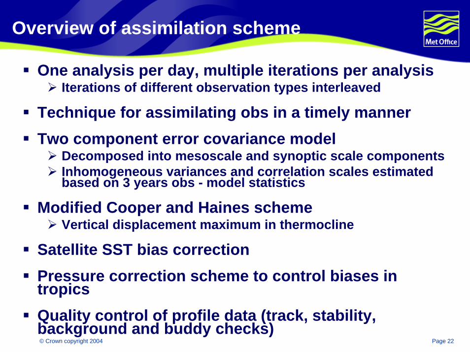
Overview of assimilation scheme
One analysis per day, multiple iterations per analysisIterations of different observation types interleaved
Technique for assimilating obs in a timely mannerTwo component error covariance model
Decomposed into mesoscale and synoptic scale componentsInhomogeneous variances and correlation scales estimated based on 3 years obs - model statistics
Modified Cooper and Haines schemeVertical displacement maximum in thermocline
Satellite SST bias correctionPressure correction scheme to control biases in tropicsQuality control of profile data (track, stability, background and buddy checks)

© Crown copyright 2004 Page 23
Troubleshooting
© Crown copyright 2004 Page 24
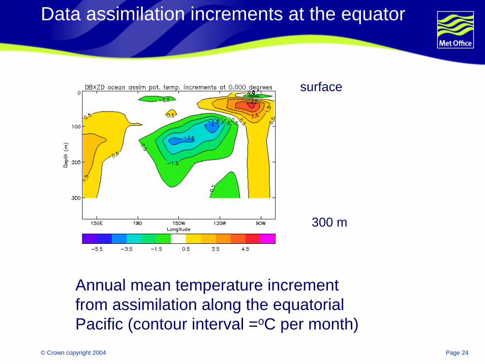
Data assimilation increments at the equator
surface
300 m
Annual mean temperature increment from assimilation along the equatorial Pacific (contour interval =oC per month)

© Crown copyright 2004 Page 25
Effect of simple data assimilation
surface
400 m
No assimilation With assimilation
Annual mean vertical velocities at 110 oW (5 oN to 5 oS) contour interval = 10-3 cm/s = 100 m/day
© Crown copyright 2004 Page 26
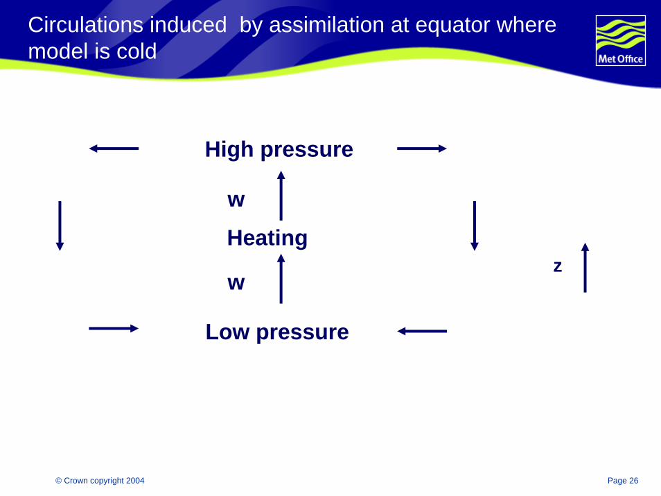
Circulations induced by assimilation at equator where model is cold
High pressure
w
Heatingz
w
Low pressure

© Crown copyright 2004 Page 27
Balance of forces along equator in Eastern Pacific
Surface winds
Surface slope
Thermocline slope
z
With assimilationNo assimilationEast
© Crown copyright 2004 Page 28
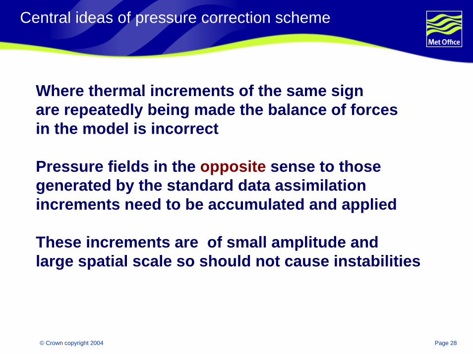
Central ideas of pressure correction scheme
Where thermal increments of the same sign are repeatedly being made the balance of forcesin the model is incorrect
Pressure fields in the opposite sense to thosegenerated by the standard data assimilation increments need to be accumulated and applied
These increments are of small amplitude and large spatial scale so should not cause instabilities
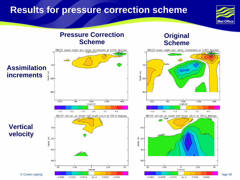
© Crown copyright 2004 Page 29
Results for pressure correction scheme
Assimilationincrements
Verticalvelocity
Pressure CorrectionScheme
OriginalScheme
© Crown copyright 2004 Page 30
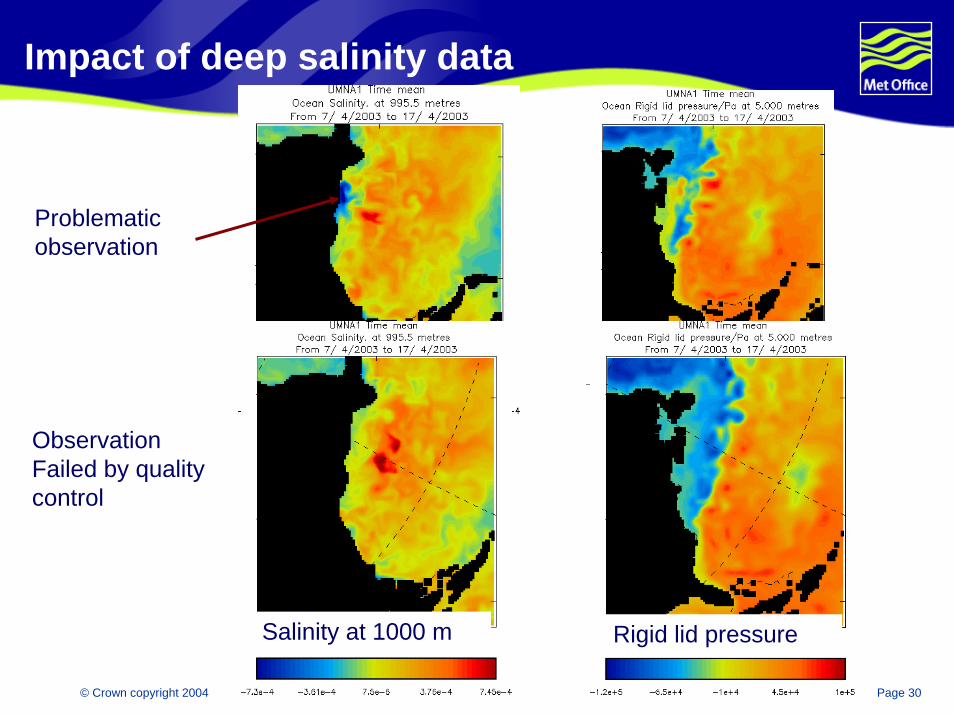
Impact of deep salinity data
Problematicobservation
Salinity at 1000 m
ObservationFailed by qualitycontrol
Rigid lid pressure
© Crown copyright 2004 Page 31
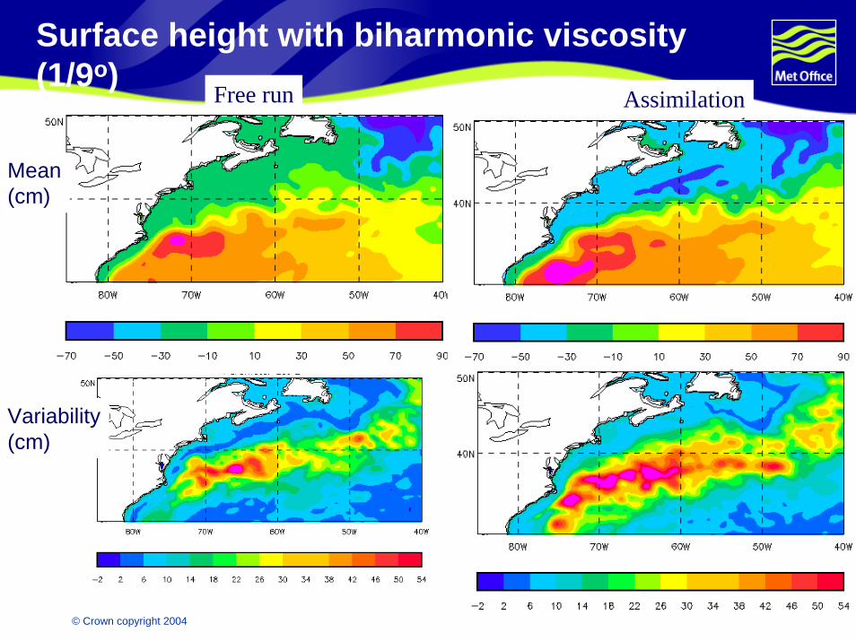
Surface height with biharmonic viscosity (1/9o)
Free run
Mean(cm)
Variability(cm)
Assimilation
© Crown copyright 2004 Page 32
Impact of viscosity on Gulf Stream
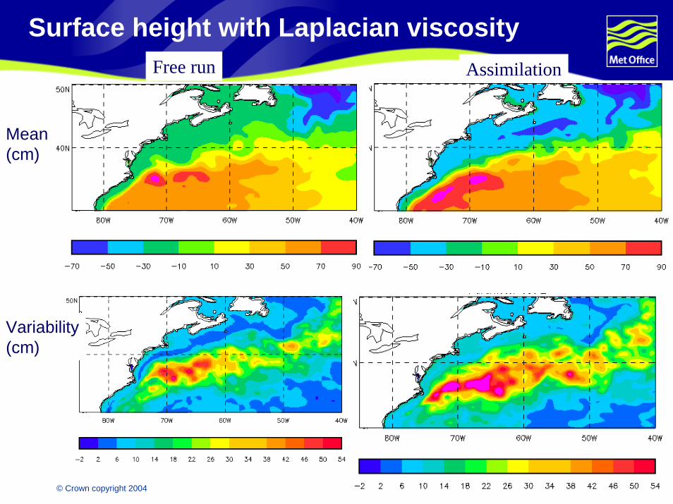
Chassignet & Garraffo found separation of 1/12o MICOM isopycnal model to be sensitive to formulation of viscosityJust biharmonic viscosity gave too much mesoscaleactivity and unsatisfactory separationJust Laplacian viscosity improved separation, but not enough penetration of Gulfstream jetBest results with combination of biharmonic and LaplacianviscosityDave Storkey repeated experiments with effectively Laplacian viscosity
© Crown copyright 2004 Page 33
Surface height with Laplacian viscosity
Mean(cm)
AssimilationFree run
Variability(cm)

© Crown copyright 2004 Page 34
Assessments
© Crown copyright 2004 Page 35
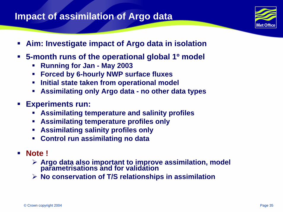
Impact of assimilation of Argo data
Aim: Investigate impact of Argo data in isolation5-month runs of the operational global 1º model
Running for Jan - May 2003 Forced by 6-hourly NWP surface fluxesInitial state taken from operational modelAssimilating only Argo data - no other data types
Experiments run:Assimilating temperature and salinity profilesAssimilating temperature profiles onlyAssimilating salinity profiles onlyControl run assimilating no data
Note !Argo data also important to improve assimilation, model parametrisations and for validationNo conservation of T/S relationships in assimilation
© Crown copyright 2004 Page 36
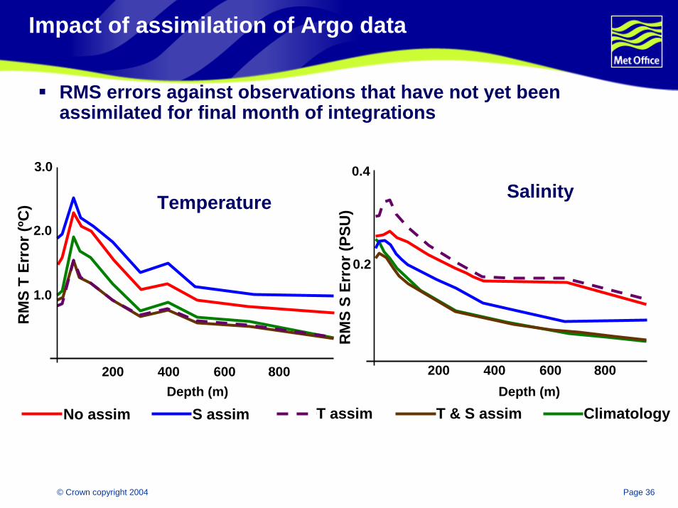
Impact of assimilation of Argo data
RMS errors against observations that have not yet been assimilated for final month of integrations
Temperature Salinity
RM
S T
Erro
r (ºC
)
RM
S S
Erro
r (PS
U)
1.0
2.0
3.0
0.2
Depth (m) Depth (m)200 400 600 800 200 400 600 800
No assim S assim T assim T & S assim Climatology
0.4
© Crown copyright 2004 Page 37
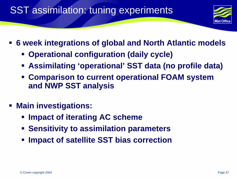
SST assimilation: tuning experiments
6 week integrations of global and North Atlantic modelsOperational configuration (daily cycle)Assimilating ‘operational’ SST data (no profile data)Comparison to current operational FOAM system and NWP SST analysis
Main investigations:Impact of iterating AC schemeSensitivity to assimilation parametersImpact of satellite SST bias correction
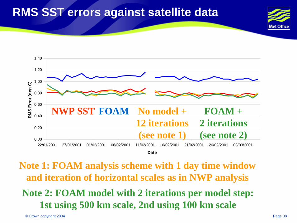
© Crown copyright 2004 Page 38
RMS SST errors against satellite data
Figure 3
0.00
0.20
0.40
0.60
0.80
1.00
1.20
1.40
22/01/2001 27/01/2001 01/02/2001 06/02/2001 11/02/2001 16/02/2001 21/02/2001 26/02/2001 03/03/2001
Date
RM
S Er
ror (
deg
C)
NWP SST FOAM No Model + 12 its Model + 2its
NWP SST FOAM No model +12 iterations(see note 1)
FOAM +2 iterations(see note 2)
Note 1: FOAM analysis scheme with 1 day time windowand iteration of horizontal scales as in NWP analysis
Note 2: FOAM model with 2 iterations per model step: 1st using 500 km scale, 2nd using 100 km scale
© Crown copyright 2004 Page 39
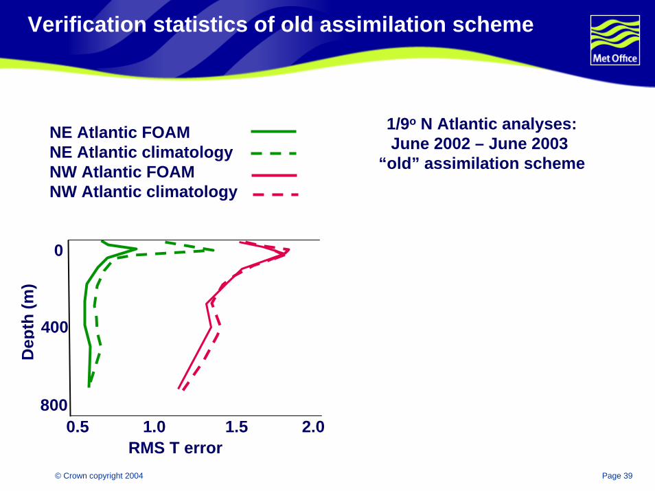
Verification statistics of old assimilation scheme
1/9o N Atlantic analyses:June 2002 – June 2003
“old” assimilation schemeChNE Atlantic FOAM
NE Atlantic climatologyNW Atlantic FOAMNW Atlantic climatology
Dep
th (m
)
800
0
400
RMS T error0.5 1.0 1.5 2.0
© Crown copyright 2004 Page 40
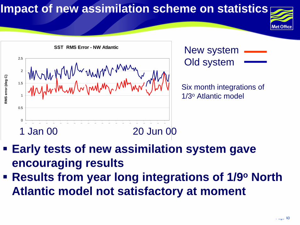
Impact of new assimilation scheme on statistics
SST RMS Error - NW Atlantic
0
0.5
1
1.5
2
2.5
01/0
2/20
00
08/0
2/20
00
15/0
2/20
00
22/0
2/20
00
29/0
2/20
00
07/0
3/20
00
14/0
3/20
00
21/0
3/20
00
28/0
3/20
00
04/0
4/20
00
11/0
4/20
00
18/0
4/20
00
25/0
4/20
00
02/0
5/20
00
09/0
5/20
00
16/0
5/20
00
23/0
5/20
00
30/0
5/20
00
06/0
6/20
00
13/0
6/20
00
20/0
6/20
00
RM
S er
ror (
deg
C)
vs in situ - new system vs in situ -old system
New system Old system
1 Jan 00 20 Jun 00
Early tests of new assimilation system gave encouraging resultsResults from year long integrations of 1/9o North Atlantic model not satisfactory at moment
Six month integrations of 1/3o Atlantic model

© Crown copyright 2004 Page 41
Changing Priorities

© Crown copyright 2004 Page 42
Changing context
FOAM project proposed to Navy in 1985 by Howard Cattle and Adrian Gill during Cold War
By 1995 Navy requirement for high resolution open ocean forecasts had diminished; forecasts of shelf seas and coastal waters main priority
GODAE started in 1997. Demonstration motivated by need to transition ocean satellites to operational funding
© Crown copyright 2004 Page 43
Changing context: last 5-10 years
Consolidation of freely available ocean community models and user groups
Software for Earth system models (e.g. OASIS coupler and PRISM) emerging
Need for sustainable management of ocean environment, particularly near coast, recognised (GMES program of EC and ESA)
Building on GODAE, Mersea project is strengthening coordination and collaboration in Europe

© Crown copyright 2004 Page 44
Transition to NEMO
NEMO=Nucleus for European Modelling of Ocean
Jointly owned by consortium who undertake to maintain and develop it (CNRS, Mercator, Met Office)
Free-ware
Initial version is based on OPA
Will be developed for shelf seas (in collaboration with POL)
Met Office will transition climate simulations, seasonal forecasting and short-range forecasting to this system
© Crown copyright 2004 Page 45
Broadening Applications
We have set up an Ocean Customer Group containing representatives of
DEFRA (Environment, Food and Rural Affairs)Environment AgencyMaritime Coastguard AgencyDTI (Trade and Industry)oil companies
Seeking to build joint programs to support their activities, particularly on European Shelf
What will be the main use of deep ocean forecast systems ?
Coupled two-week ensemble atmospheric forecasts ? Boundary data for shelf models ?Monitoring of climate circulation (e.g. THC) ?
© Crown copyright 2004 Page 46
National Centre for Ocean Forecasting
We will become UK’s National Centre for Ocean Forecasting
In association with NERC labs:
POL, PMLSOC, ESSC
Strengthens and recognises need for science base for operational ocean forecasting
Improves our visibility

© Crown copyright 2004 Page 47
Short-term priorities
Improvement of mesoscale surface currents; altimeter assimilation in high resolution models; investigation/demonstration of forecast skill
Transition to NEMO
Improvement of mixed layer forecasts
Development of sea-ice assimilation
Deep ocean ecosystem, ocean colour assimilation, air-sea CO2 flux (CASIX)

© Crown copyright 2004 Page 48
Questions & Answers
Recommended


![A Dimensions: [mm] B Recommended land pattern: [mm] D ... · 2013-03-12 2013-01-13 2012-12-10 2012-10-29 2012-08-27 2006-05-05 DATE SSt SSt SSt SSt SSt SSt SSt BY SSt COt COt SSt](https://img.pdfslide.us/doc/110x75/604b228bc93c005c75431c51/a-dimensions-mm-b-recommended-land-pattern-mm-d-2013-03-12-2013-01-13.jpg)