The Effects of Redistricting on Incumbents
CitationAnsolabehere, Stephen, and James M. Snyder, Jr. 2012. "The Effects of Redistricting on Incumbents." Election Law Journal: Rules, Politics, and Policy 11(4): 490-502.
Published Versiondoi:10.1089/elj.2012.0152
Permanent linkhttp://nrs.harvard.edu/urn-3:HUL.InstRepos:11910880
Terms of UseThis article was downloaded from Harvard University’s DASH repository, and is made available under the terms and conditions applicable to Open Access Policy Articles, as set forth at http://nrs.harvard.edu/urn-3:HUL.InstRepos:dash.current.terms-of-use#OAP
Share Your StoryThe Harvard community has made this article openly available.Please share how this access benefits you. Submit a story .
Accessibility
The Effects of Redistricting on Incumbents1
Stephen Ansolabehere
Department of Government
Harvard University
James M. Snyder, Jr.
Departments of Political Science and Economics
Massachusetts Institute of Technology
August, 2012
1Paper to be presented at the Voting Power in Practice Workshop at the University of Caen,1-3 July 2008, sponsored by the Leverhulme Trust (Grant F/07-004/AJ).
Abstract
We analyze the effects of redistricting on the electoral fortunes of incumbent legislators, usingvoting data on U.S. congressional districts, state legislative districts, and statewide races.We find little evidence that redistricting helps incumbents in U.S. legislative elections. Ifanything, redrawing district lines reduces the average vote margin of those in districtedoffices compared with offices that are not districted, reduces electoral security, and increasesturnover in the legislature.
1. Introduction
Over the past 50 years U.S. elections have witnessed the rising importance of incumbency.
While party remains the central and most important predictor of voting behavior, American
voters now also base their decisions on the individuals running for office and what those
individuals have done to serve local interests. Sitting legislators, when they run for reelection,
evidently enjoy substantial electoral advantages, which are manifest both in voters’ behavior
and in aggregate rates of electoral competition and legislative turnover. For their part, voters
favor incumbents, and as a result incumbents today receive vote margins approximately 10
percentage points greater than candidates running in open seats. Aggregate turnover in
U.S. legislative elections has similarly fallen. Many fewer incumbents retire today than in
previous generations; reelection rates of those who do run for reelection exceed 90 percent.
As a result, turnover in U. S. legislatures is extremely low and the tenure of the typical
legislator grows longer.
The rising advantages of incumbency, whatever their causes, have altered the patterns
of representation and electoral responsiveness in the U.S. The incumbency effect has muted
the effects of short-run factors, such as economic fluctuations, on the composition of U.S.
legislatures (Mayhew, 1974). It has insulated the majority party in Congress and length-
ened the time that the majority party can expect to remain in power (Ansolabehere and
Gerber, 1997). It is thought to reflect a lack of collective responsibility inside the legislature,
especially where matters of budgeting are concerned (Fiorina, 1980).
Why American legislators win reelection at such high rates remains an unsolved puzzle.
Here we examine one of the most enduring and controversial conjectures – namely, that
redistricting accounts for the rise of incumbent-centered politics. Incumbency arose at same
time as redistricting revolution in the U.S., set off by the landmark U.S. Supreme Court case
Baker v. Carr.1 That case, decided in March, 1962, led to the redrawing of nearly every U.S.
House and states legislative district in America within a four year span.2 Research in political
science identifies this as precisely the time period with the steepest rise in incumbents’ vote
1For a history of that case and its consequences see Ansolabehere and Snyder (2008).2Ibid, page 187.
2
margins (Jacobson, 1987). The coincidence of rising incumbency advantages and widespread
court-mandated redistricting has led many observers to conclude that the two are inextricably
linked.
Three specific arguments claim a causal relation between redistricting and incumbency.
First, incumbents use redistricting to create safe (partisan) seats. Perhaps the clearest
statement of this argument comes from the Samuel Issacharoff (2002), who likens redistricting
to the foxes guarding the hen house. The two major parties, he argues, engage in duopolistic
behavior to guarantee their continued dominance of American elections by creating large
numbers of safe Democratic and safe Republican seats.3 Second, incumbents use redistricting
to protect their own seats. Redistricting turns the normal representation process on its
head. It is at this moment that politicians choose their constituencies, rather than the
constituencies choosing the politicians. That opportunity might allow incumbents to create
districts that are particularly favorable to them on personal grounds. Third, redistricting
creates incumbency advantages by creating barriers to entry for challengers. Political control
of redistricting allegedly gives incumbents another instrument with which to deter entry. As a
result, new district boundaries are thought to increase legislators’ vote shares. Note that this
argument is distinct from traditional partisan gerrymandering, in which the majority party
creates more seats for itself by “packing” voters of the opposition party. Under partisan
gerrymandering seats held by the minority party’s incumbents will tend to get safer, but
districts held by the majority party’s incumbents may become more competitive.4
Alan Ehrenhalt, executive editor of Governing magazine, offered the following succinct
assessment:
“Decades of litigation and judicial activism have created a system in which bizarrely
shaped districts exist to serve undisguised racial purposes. Partisan gamesmanship has
brought us legislatures stacked with safe seats that preclude competition at election time.
All of this has taken place under the auspices of a Supreme Court doctrine that virtually
any political outrage is permissible as long as the census populations of the districts are
3See especially, Issacharoff, op cit, page 598. See also, Cox and Katz (2002). For other arguments, see,e.g. Coate and Knight (2007).
4See Butler and Cain (1992) for a discussion of these distinctions.
3
mathematically the same – even though no such mathematical precision even exists.”5
These arguments represent an important line of thinking about the political consequences
of allowing legislators to draw district boundaries. In one sense, they are right. An obvious
conflict of interest arises when a politician chooses his or her constituency, and legislators
devote considerable effort to influence the composition of their districts. The presence of
such a conflict of interest does not translate necessarily into a political advantage, however.
What actually happens to incumbents around redistricting is quite a different picture.
Redistricting is a disruptive factor, for incumbents and parties. Looking at electoral outcomes
across redistricting periods we conclude that periodic redistricting forced by the courts since
the 1960s has, on the whole, weakened incumbency and partisan electoral advantages.
We examine five key indicators of the consequences of political control over electoral
institutions. The first is the partisanship of districts. Insulation of incumbents and of
the incumbent party predicts that most districts are either overwhelmingly Democratic or
overwhelmingly Republican, with few mixed or moderate constituencies. Using conventional
measures we show that the opposite is true – most districts are moderate and there is no or
little bimodality in the distribution of districts’ partisanship.
The second indicator is vote differentials between “new” and “old” parts of incumbents’
districts. Changes in district boundaries hurt incumbents since they lose voters whom they
had served and gain voters who don’t know them. There is, in fact, a large difference
between the votes that incumbents win among familiar and new parts of their districts. (See
Ansolabehere, Snyder, and Stewart 2001.)
The third indicator is the incumbency effect on the vote, estimated either using regression
analysis or sophomore surge. The incumbency effect is defined as the expected difference
between the vote share won by a party when an incumbent is running and when an incumbent
is not running. This quantity can be estimated for any type of office, such as all U. S.
House elections or all U. S. Senate elections. (See Erikson 1971; Gelman and King 1990)
We compare the incumbency effects for offices that are districted and offices that are not
districted, and find that the incumbency effect is in fact much smaller in districted elections
5Alan Ehrenhalt, “Frankfurter’s Curse,” Governing, January 2004 (www.governing.com).
4
(state legislatures and the U.S. House) than in non-districted elections (U.S. senate, governor,
and other statewide offices).
The fourth indicator is changes in district partisanship. We find small changes in parti-
sanship, and in the case of Democrats, changes that hurt incumbents on average rather than
help them. Persily (2002) makes a similar observation in response to Issacharoff.6
Finally, we examine turnover. If redistricting amounts to incumbency protection then
there should be little or no turnover in the elections following the creation of new constituen-
cies. In fact, redistricting years regularly show the highest turnover.
We present a series of statistical analyses and show that in one analysis after another
the data do not break in the direction one would expect if incumbents were able to carefully
control the process and carve up the electoral terrain to their benefit. There are, of course,
exceptions to this overall picture, but the typical state legislator or member of Congress
dreads the redistricting process. It disrupts relations that the legislature has built up with
a constituency over the course of a decade. Those disruptions, though, are a necessary part
of democratic politics; they are required in order to allow Congress and state legislatures to
evolve with the ever changing American electorate.
2. Partisanship of Districts
There are really two distinct arguments. The first alleges that incumbents of both parties
have raised their electoral security by crafting safe partisan districts, with overwhelming
numbers of Democrats or of Republicans. The second claims that incumbents are able to
increase their personal vote through the redistricting process. In this section we turn to the
first of these two conjectures. We examine the second possibility in the sections that follow.
Isaacharoff, writing in the Harvard Law Review, offers the most cogent expression of this
idea, which he calls duopolistic gerrymandering. The two parties he argues have formed
something of a cartel, a duopoly through which they decide to divide the political turf to
suit each party’s interest and fend off all potential entrants into their market. Most states are
6On it’s own, Persily’s criticism may not hold much force, as one might argue that legislators’ involvementin redistricting prevented their districts from becoming even worse. However, the fact that commissions andcourts produce very similar results to legislature-drawn maps suggests that incumbents have relatively littleability control their own fates through the redistricting process.
5
closely divided between the parties. Arbitrarily drawn districts would create a large number
of districts that are split evenly between Democratic and Republican adherents, and with a
good dose of Independent voters thrown in as well. For politicians, this would be a terrible
state of affairs as competitive districts are difficult to win and hard to hold onto. Democratic
and Republican legislators, realizing this problem, may join forces and divide their state so
that most seats are safe for one party or another, leaving only a handful of evenly split,
competitive districts. Focusing on the facts in Gaffney v. Cummings, Issacharoff argues
that the ”conceptual weakness in how the Court has treated the potential for mischievous
manipulation of redistricting is evident in ... a political compromise between the Democrats
and Republicans of Connecticut to partition the state so as to lock in the political status
quo ante.”7
This is a nice argument. Sitting legislators can improve their own political positions and
reduce the risk facing their party. Duopolistic gerrymandering buys the support of the large
majority of sitting legislators since the large majority of them are guaranteed safe (partisan)
seats. Such a plan minimizes the electoral uncertainty and electoral costs that the parties’
face, since competition is limited to a few places. It does not cause incumbency advantages,
but it would have the side effect of protecting those incumbents who happen to be in safe
Democratic and safe Republican seats. It would, if real, deepen the partisan division among
the constituencies that the legislators represent and further polarize of the parties inside
the legislature. Of course it assumes that the members of the minority party would prefer
to remain a permanent legislative minority, safe in their own seats but with little hope of
gaining control of the house.
This is not just the stuff of academic debates. It is widely believed to be the new reality.
Jeffrey Toobin, writing in the New Yorker magazine, has called this “The Great Election
Grab.” Republican congressman James Leach of Iowa said of Congress in 2003 that “a little
less than 400 seats are totally safe.” Even those who had once defended the current process
now think it broken. The sharp increases in incumbent departures following redistricting cast
a shadow of doubt over this conjecture. Patterns of defeat increase those doubts still further.
7Issacharoff op cit, page 598.
6
It is indeed true that in the typical election only one in ten seats are highly competitive,
the set of close elections varies from year to year - hardly what one would expect from a
carefully crafted set of boundaries. Indeed, three years after Congressman Leach offered his
assessment, the voters bounced Leach and 30 of his Republican colleagues, giving Democrats
control of Congress for the first time in 12 years.
The districts themselves provide direct evidence that the politicians have not been able to
capture the redistricting process in the ways that Issacharoff, Toobin, and others conjecture.
It is not that they haven’t tried, they just haven’t succeeded wholesale. Successive rounds
of duopolistic gerrymandering over the past 40 years should have created large numbers
of highly safe Democratic seats and highly safe Republican seats. The result would be a
small number of marginal districts in which the ratio of Democrats to Republicans is about
even, and a very large number of districts where the fraction of Democrats far exceeds the
fraction of Republican identifiers or vice versa. If one were to rank order the legislative
districts in the country from most Democratic to most Republican and count the frequency
of districts that were safely Democratic, marginal, or safely Republican, a two-humped or
bimodal shape would occur. Such a bimodal distribution of the underlying partisanship of
district partisanship would effectively insulate incumbents against national swings in the
two-party vote. In other words, if the distribution of district partisanship were bimodal,
then a national swing in the vote of, say 5 or 10 percentage points from the Democrats to
the Republicans or vice versa, would produce relatively few incumbent defeats.
By contrast, the districts may be drawn with little regard for or opportunity to create
safe seats or protect incumbents. The bargaining over redistricting across legislative cham-
bers and with the executive maybe so intense and subject to so many competing demands
that it leaves little leeway for party. If the lines were drawn without regard to party, the
typical district would reflect the division of the vote statewide, and the partisan division in
most of the districts would deviate only somewhat from the division of the statewide vote.
There would be a few highly Republican and highly Democratic districts. This principle
has been conjectured, at least among statisticians, for over a century. The eminent 19th
Century statistician F.Y. Edgeworth studied English Parliamentary elections with just such
7
a hypothetical district system in mind and predicted that if redistricting did not matter we
should expect a bell-shaped, or normal, curve. Under this possibility, a swing of 5 or 10
points nationwide would turn out of office relatively large numbers of incumbents. Conven-
tionally, Political Scientists have used margins of 60-40 or 55-45 to define which districts are
marginal.
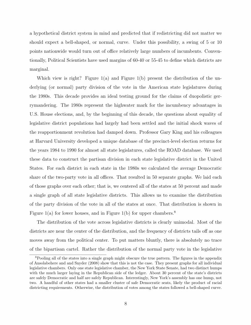
Which view is right? Figure 1(a) and Figure 1(b) present the distribution of the un-
derlying (or normal) party division of the vote in the American state legislatures during
the 1980s. This decade provides an ideal testing ground for the claims of duopolistic ger-
rymandering. The 1980s represent the highwater mark for the incumbency advantages in
U.S. House elections, and, by the beginning of this decade, the questions about equality of
legislative district populations had largely had been settled and the initial shock waves of
the reapportionment revolution had damped down. Professor Gary King and his colleagues
at Harvard University developed a unique database of the precinct-level election returns for
the years 1984 to 1990 for almost all state legislatures, called the ROAD database. We used
these data to construct the partisan division in each state legislative district in the United
States. For each district in each state in the 1980s we calculated the average Democratic
share of the two-party vote in all offices. That resulted in 50 separate graphs. We laid each
of those graphs over each other; that is, we centered all of the states at 50 percent and made
a single graph of all state legislative districts. This allows us to examine the distribution
of the party division of the vote in all of the states at once. That distribution is shown in
Figure 1(a) for lower houses, and in Figure 1(b) for upper chambers.8
The distribution of the vote across legislative districts is clearly unimodal. Most of the
districts are near the center of the distribution, and the frequency of districts tails off as one
moves away from the political center. To put matters bluntly, there is absolutely no trace
of the bipartisan cartel. Rather the distribution of the normal party vote in the legislative
8Pooling all of the states into a single graph might obscure the true pattern. The figures in the appendixof Ansolabehere and and Snyder (2008) show that this is not the case. They present graphs for all individuallegislative chambers. Only one state legislative chamber, the New York State Senate, had two distinct humpswith the much larger laying in the Republican side of the ledger. About 30 percent of the state’s districtsare safely Democratic and half are safely Republican. Interestingly, New York’s assembly has one hump, nottwo. A handful of other states had a smaller cluster of safe Democratic seats, likely the product of racialdistricting requirements. Otherwise, the distribution of votes among the states followed a bell-shaped curve.
8
districts looks to be consistent with the notion that the parties can exert relatively little
influence over the contours of legislative districts. They have some influence on the margin,
but, consistent with our earlier findings on partisan bias, state legislative districts do not
seem to reflect a strongly partisan tilt.
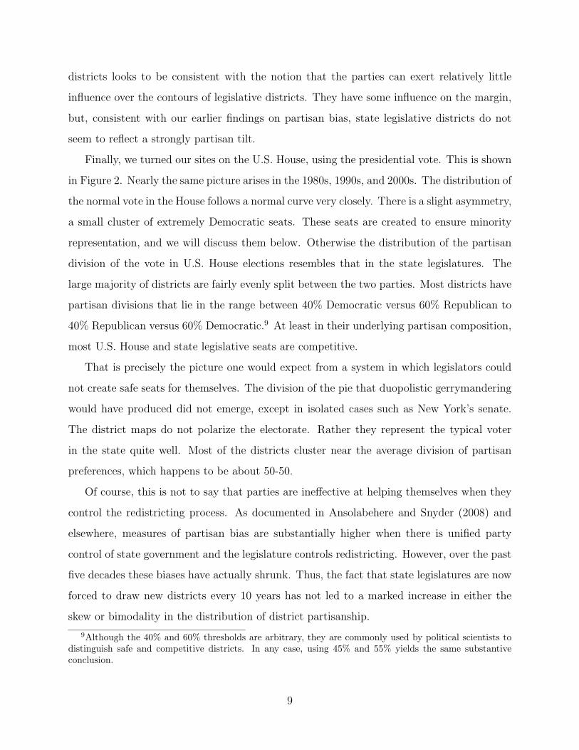
Finally, we turned our sites on the U.S. House, using the presidential vote. This is shown
in Figure 2. Nearly the same picture arises in the 1980s, 1990s, and 2000s. The distribution of
the normal vote in the House follows a normal curve very closely. There is a slight asymmetry,
a small cluster of extremely Democratic seats. These seats are created to ensure minority
representation, and we will discuss them below. Otherwise the distribution of the partisan
division of the vote in U.S. House elections resembles that in the state legislatures. The
large majority of districts are fairly evenly split between the two parties. Most districts have
partisan divisions that lie in the range between 40% Democratic versus 60% Republican to
40% Republican versus 60% Democratic.9 At least in their underlying partisan composition,
most U.S. House and state legislative seats are competitive.
That is precisely the picture one would expect from a system in which legislators could
not create safe seats for themselves. The division of the pie that duopolistic gerrymandering
would have produced did not emerge, except in isolated cases such as New York’s senate.
The district maps do not polarize the electorate. Rather they represent the typical voter
in the state quite well. Most of the districts cluster near the average division of partisan
preferences, which happens to be about 50-50.
Of course, this is not to say that parties are ineffective at helping themselves when they
control the redistricting process. As documented in Ansolabehere and Snyder (2008) and
elsewhere, measures of partisan bias are substantially higher when there is unified party
control of state government and the legislature controls redistricting. However, over the past
five decades these biases have actually shrunk. Thus, the fact that state legislatures are now
forced to draw new districts every 10 years has not led to a marked increase in either the
skew or bimodality in the distribution of district partisanship.
9Although the 40% and 60% thresholds are arbitrary, they are commonly used by political scientists todistinguish safe and competitive districts. In any case, using 45% and 55% yields the same substantiveconclusion.
9
3. Old vs. New Areas
The second form of the argument that redistricting causes incumbents’ electoral advan-
tages alleges that the districts themselves are carved up in a way that creates a personal
vote for the individual representative. That might come from the creation of a district that
contains voters loyal to the incumbent from past service and name recognition or from the
creation of a district with higher numbers of voters inclined to favor the incumbent by virtue
of party or for sociological affinities (such as ethnicity or religion).
We look at each of these factors separately. The approach in this section is to examine
how redistricting alters the constituencies represented by incumbents and, in turn, changes
their vote shares.
3.1. Changing Partisanship of Districts
One line of thinking holds that each redistricting makes marginal changes in the partisan-
ship of districts. Through successive rounds of redistricting incumbents gain more favorable
partisan compositions of their districts. One important branch in this vein reflects the polit-
ical control of the institutions that conduct or oversee the redistricting. In some states the
legislatures draw lines; in others lines are drawn by independent commissions; in still oth-
ers the duty falls to the courts. Does redistricting improve the partisan composition of the
typical incumbent’s districts? Does political control of redistricting make for more partisan
districts?
For the three most recent redistricting episodes, we measure directly the degree to which
redistricting helps incumbents by shifting the partisan composition of their districts in their
favor. We cannot directly measure party identification at the congressional district level, but
we can use the presidential vote.10
Importantly, for the three most recent episodes, voting data are available for the same
presidential election in both the old and new districts after redistricting. Specifically, the
10Many previous studies use the presidential vote to measure district partisanship, including Erikson(1971b), Cantor and Herrnson (1997), Ansolabehere, Snyder and Stewart (2000, 2001), Powell (2000), Ja-cobson (2004), and Abramowitz, Alexander and Gunning (2006). It is not perfect, of course, but it isprobably the best single measure available at the congressional district level.
10
results of the 1980 presidential election are available for the districts that applied in 1980
and also the districts that applied in 1982; the results of the 1988 election are available for
the both the 1990 and 1992 districts; and the results of the 2000 election are available for
both the 2000 and 2002 districts.
Given this data, the analysis is straightforward and proceeds as follows. Fix a par-
ticular redistricting episode. Let V Bi be the Democratic percentage of the two-party vote
in the relevant presidential election in incumbent i’s district before redistricting, let V Ai
be the Democratic percentage of the two-party vote in the relevant presidential election
in incumbent i’s district after redistricting, and let ∆i = V Ai − V B
i . Let SD (SR) be the
set of districts held by Democratic (Republican) incumbents running for reelection in the
year after redistricting, and let ND (NR) be the number of districts in SD (SR). Finally,
let ∆D = (1/ND)∑
i∈SD∆i and let ∆R = −(1/NR)
∑i∈SR
∆i (note the reversal of sign for
Republican incumbents). These last quantities are the main quantities of interest, and pro-
vide measures of the average extent of pro-incumbent or anti-incumbent partisan shifts in
districts. In both cases, positive values imply changes in district partisanship that favor
incumbents.
The results are shown in Table 1. We find that, on average, redistricting slightly helps
Democratic incumbents in terms of district partisanship, and slightly helps Republican in-
cumbents. Specifically, districts held by Democratic incumbents become about 0.5 percent-
age points less Democratic after redistricting, and districts held by Republican incumbents
become about 1 to 1.5 percentage points more Republican. Neither of these changes is over-
whelming. That is, those drawing district lines indeed try to help incumbents, but the effects
are on the order of 1 percentage point.
Finally, there is the question of agency. Who does the redistricting might determine
the effects on the electoral process. Table 2 considers whether it matters if redistricting
is done by state legislatures, commissions, or courts.11 Carson and Crepsin (n.d.) argue
that plans drawn by commissions and courts generally lead to more electoral competition
than those drawn by state legislatures. Overall, we find little differences with respect to
11We use the coding in Appendix Table A in Carson and Crespin (n.d).
11
changes in district partisanship. In none of the four rows are the F-statistics for tests of the
equality of the three cell means statistically significant from zero at the .05 level.12 The one
noticeable difference is for Democratic incumbents under court-ordered plans (row 1 and row
3). In this case district partisanship shifts against the incumbent by more than 1 percentage
point, on average, while under legislative or commission plans the changes are minimal. On
the other hand, court-ordered plans are not much different than other types for Republican
incumbents. Thus, the findings by Carson and Crespin are likely due to factors other than
district partisanship, such as race or ethnicity.
Table 3 takes a closer look at the plans drawn by state legislatures, divided according to
the party in control of the state government at the time of redistricting. A state is under
Democratic control if Democrats have a majority in both houses of the state legislature the
governor is a Democrat, or if Democrats have veto-proof majorities in both houses of the state
legislature. Republican control is defined analogously, and the remaining cases are classified
as Divided. There is some evidence of “packing” in Table 3. Democratic incumbents are
helped by redistricting when Republicans control the state government, but not in other
cases. Also, while Republican incumbents are helped in all cases, they are especially helped
when Democrats control the state government. In all four rows of the table the F-statistics
for tests of the equality of the three cell means are statistically significant from zero at the
.05 level.
Note that the analyses above focus on incumbents who run for reelection. Thus, they
may understate the degree to which redistricting hurts incumbents. This would be the case,
for example, if redistricting also induces retirements, especially among incumbents whose
districts shift more sharply against them. The following quote is illustrative: “Wolpe decided
against either of two unpalatable alternatives: a primary fight against Democrat Bob Carr
in the 8th, or a run in the new 7th, which was at least 5% more Republican than his old seat
and in which about half the voters had no acquaintance with the hard-driving constituency
service which has offset his liberal voting record.”13 In future work we will analyze data on
12The differences in the first row – for Democratic incumbents in states with two or more districts – issignificant at the .10 level.
13From the Almanac of American Politics, 1994 (page 651).
12
the districts in which retiring incumbents would have run had they run for reelection, which
will allow us to check this.
To the extent that we find that redistricting increases the partisan vote share of incum-
bents, the effects are small. On average, a typical Democratic incumbent’s average district
partisanship increases by .5 percentage points, and a typical Republican incumbent’s average
district partisanship increases by 1 percentage point. When one party controls the entire
process the effects are somewhat larger for some seats. The dominant party does not change
appreciably the average partisanship of it’s own incumbents’ districts, but it does pack the
opposition somewhat, by increasing the average partisanship of the out party’s incumbents
by about 2 percentage points. When control is divided the changes in district partisanship
are quite small, and only Republican incumbents appear to benefit. On average, Democratic
incumbents lose slightly. Thus, the changes in district partisanship are not consistent with
bipartisan gerrymandering along the lines alleged in the Connecticut redistricting challenged
under Gaffney v. Cummings. If anything, they are more consistent with claims of partisan
gerrymandering.
This is not to say that instances of bipartisan gerrymandering never arise. But, even
under divided government, such cases are evidently exceptions, not the norm. To the extent
there is any evidence that gerrymandering affects the underlying partisanship of districts
it is of old-fashioned variety – packing the out-party – rather than duopolistic, cartel-like
division of the electoral terrain “to preserve status quo ante.” Even these effects, however,
are quite small and not systematic.
3.2. Changing Personal Votes
An alternate line of thinking holds that redistricting might increase the personal vote for
the representative. One view of the incumbency effect holds that it reflects personal support
in the district arising through such factors as name recognition, constituency service, and
a voting record tailored to local voters’ preferences (Cain, Ferejohn, and Fiorina, 1987).
Redistricting might increase the personal vote of incumbents by shaving off precincts where
the incumbent has the weakest personal support.
13
Changes in districts have been used in past studies to capture the extent of the personal
vote. Following redistricting many districts consist of areas that the legislator previously
represented and areas that the legislator had not represented in the past – old voters and
new voters. Controlling for the partisanship of the areas, the difference in the incumbent’s
vote share between old areas and new areas in the election following redistricting will reflect
the extent of the personal vote (see, e.g., Fiorina, 1974; Rush, 1993; Ansolabehere, Snyder,
and Stewart, 2000). As Ansolabehere, Snyder and Stewart (2000) note, when new areas are
added to an incumbent’s district, the incumbent will initially have far less name recognition
in the new area, and fewer voters in the new area will know about the incumbent’s prior
constituency service, voting record, etc.14 From the incumbents’ point of view, these new
areas are unknown, potentially hostile areas that require extra attention and investment to
win over.
Analysis of the difference in vote between old voters and new voters suggests that the
personal vote accounts for approximately half of the incumbency effect. The overall incum-
bency effect in a typical U. S. House race is approximately 8 to 10 percent and the estimate
of the personal vote from the analysis of old and new areas is approximately 4 to 5 percent.15
The comparison of old voters and new voters suggest that redistricting itself hurts in-
cumbents to the extent that it changes their constituencies, thereby lowering the size of the
personal vote. That fact, combined with the result that gains in partisan support tend to
be small, suggests that redistricting itself tends to lower the normal avenues through which
incumbents might gain electorally – that is through the partisan vote and the personal
vote. Rearranging election boundaries, then, undermines the incumbency advantage at the
micro-level. We turn next to the macro-level.
4. Comparing the U.S. House with Other Offices
The comparison of elections across episodes of redistricting suggests that redistricting
tends to lower levels of electoral support and loyalty. This suggests that the incumbency
14McKee (2008) finds lower levels of name recognition of House incumbents among survey respondents inareas that are redrawn during districting.
15See Ansolabehere, Snyder and Stewart (2000). There is some evidence that the incumbency effect is notlinear, being smaller in districts that are overwhelmingly of one party (Krashensky and Milne 1993).
14
effect overall is muted, not inflated, by redistricting. Another way to check this is to compare
offices that are districted with those those that are not. Statewide offices – U.S. senator,
governor, attorney general, secretary of state, treasurer and so on – are never redistricted.
If redistricting were the main cause of the incumbency advantage, we would expect these
offices to exhibit a small incumbency effect, or none at all.
In fact, the incumbency advantage is a general phenomenon, not one limited to offices
chosen from districts. While the incumbency advantage was first noted in U.S. House elec-
tions, early studies also documented its presence in U.S. Senate elections and gubernatorial
elections – offices that are not districted. Subsequent studies have found that the incumbency
advantage exists in nearly every elected state office in the United States (e.g., Ansolabehere
and Snyder, 2002). Moreover, incumbency advantages rose in every office from 1940 to
the present, including those not districted. The incumbency advantages for offices ranging
from governor and U.S. senator to State Auditor and state commissioners rose at the same
time and at the same rate. In the 1940s all offices had relatively small incumbency ad-
vantages, of about 2 percentage points. During the 1950s, those advantages began to grow
and their growth accelerated in the 1960s, reaching about 7 percent by 1970. The incum-
bency advantage has continued to creep up, rising to about 10 percent in the 1980s and
1990s. The accelerated growth of the incumbency advantage during the 1960s leads many to
point to reapportionment as the culprit. However, those offices not subject to redistricting
saw the same pattern of growth. The incumbency advantage is also noticeably larger for
these statewide offices than for state legislatures. The coincidence between the rise of the
incumbency advantage and the reapportionment cases appears to be just that, a coincidence.
In Figure 3 we reproduce an updated version of one of the figures in Ansolabehere and
Snyder (2002). It shows the incumbency advantage, measured using the method in Levitt
and Wolfram (1997), for U.S. House races, “higher” statewide offices, and “lower” statewide
offices.16 We estimate the incumbency advantage for each group separately for each decade.
The three curves track one another closely, except in the past two decades where the incum-
16Higher statewide offices are U.S. senator, governor, lieutenant governor, attorney general and secretary ofstate. The lower offices are treasurer, auditor, controller, comptroller, school superintendent, commissionerof agriculture, commissioner of corporations, commissioner of public utilities, commissioner of insurance,commissioner of mines, commissioner of labor, and commissioner of lands.
15
bency effect for U.S. House races drops off sharply compared to the higher statewide offices.
Redistricting is clearly not the main force driving the growth and current high level of the
incumbency effect for the statewide offices, since these are never redistricted.
Redistricting, then, is not a cause of incumbency effects, nor does it increase vote margins.
Instead, redistricting lowers incumbents vote margins, and the more a legislator’s district
changes, the worse he or she can expect to do at the polls.
5. Turnover
Incumbency-centered politics concerns more than just the expected vote received by
candidates running for office; it shapes the overall rate of turnover and career lengths of
politicians. Arguments that redistricting increases electoral security ultimately turn on the
notion that politicians craft constituency boundaries to keep themselves in office, regardless
of their electoral margins. Turnover offers the ultimate proof that redistricting on average
hurts incumbents.
Consider the U.S. House of Representatives. Let Et be the percentage of representatives
who “exit” in year t (i.e., t is the election year of their last congress).17 Figure 1 shows a graph
of Et over time. There are usually large spikes upward during redistricting episodes, which
are indicated in the figure with year numbers rather than circles. The figure also reveals the
large overall decline in turnover that has occurred in the U.S. House, a phenomenon that
has been discussed at length in the congressional literature.
A simple regression confirms what the graphs show. Let Rt =1 if t is a year ending in zero
and 0 otherwise; so, R denotes the last election year prior to a congressional reapportionment.
We also set Rt = 1 for 1964 because of court-ordered redistrictings following the Baker v.
Carr decision.18 We regress E on R and also include a third-order polynomial in t to
capture trends such as increasing professionalization and the increasing electoral advantages
17We begin the analysis in 1912 because the size of the House has been constant at 435 since then, exceptfor 1959-1962 when the number of representatives was temporarily expanded to 437 following the admission ofAlaska and Hawaii as states. We adjust accordingly in computing Et. If a representative has non-contiguousperiods of service, he or she will have multiple exits, one for each period.
18In 1964 in Wesberry v. Sanders the Supreme Court held that all congressional districts must adhere tothe one-person-one-vote standard. Almost all states redistricted during the second half of the 1960s, somemore than once.
16
of incumbency. The results are shown in the first column of Table 4. The estimates imply
that the probability of an exit is 5 percentage points higher in the last year prior to a
reapportionment. Since the average exit rate over the period under study was about 20
percent, in relative terms the effect of reapportionment is substantial – on the order of 25
percent.
Figure 2 shows an analogous graph for state legislatures, aggregating across both upper
and lower chambers. The second column in Table 1 shows the analogous regression. The
estimated effect of redistricting is similar to that for the U.S. House, about 5 percentage
points. Note also that the effects of redistricting are clearest in the post-Baker period.19
Note also that, as in the case of the U.S. House, average turnover in state legislatures has
dropped sharply over time.
6. Conclusions
Redistricting has long been thought to create the conditions that favor incumbents in
elections. That line of thinking, we find, lacks empirical support. Redistricting actually low-
ers incumbency advantages and vote margins and increases turnover, rather than the other
way around. We have further focused on one important, recent line of thinking about the dis-
tricting process – namely that the current process protects incumbents through widespread
bipartisan gerrymanders that have made districts less responsive and have even produced
the incumbency advantage. A closer look at the key empirical indicators of electoral com-
petition – including the number of competitive districts, the degree of bimodality or spread
in the distribution of district partisanship, and the effects of the districting process on the
partisanship of incumbents’ districts – reveals little or no evidence consistent with the no-
tion that incumbents systematically engage in bipartisan gerrymanders or that bipartisan
gerrymanders have created a bimodal or skewed distribution of district partisanship. This is
not to say that individual legislators and parties do not try mightily to shape the districts in
their favor. They surely do. Rather, the evidence presented here suggests that incumbency
protection is difficult to accomplish. There may be some districts successfully drawn to pro-
19In 1964 in Reynolds v. Sims the Supreme Court held that all state legislative districts must adhere tothe one-person-one-vote standard.
17
tect incumbents, but the overall picture of legislative districting does not bear that out as a
systematic consequence of the redistricting process.
We might hope that by presenting a large number of empirical problems with the argu-
ment, we might succeed in putting it to rest. This would probably be overly optimistic, since
we are not the first to disconfirm the argument. In the 1970s, influential papers by Ferejohn
(1977) and others showed no link between these two phenomena. Several papers in the 1980s
also looked for the smoking gun that redistricting inflated the incumbency effect, but found
none. Even the best evidence mustered by advocates of a connection between redistricting
and incumbency accounts for only about a 2 percent effect and, then only under the right
circumstances. The overall incumbency effect is usually estimated to be in the range of 8 to
10 percentage points.
The link between redistricting and incumbency advantages has strong intuitive appeal.
The argument gained currency in the mid 1970s shortly after the redistricting revolution of
the 1960s and the observation of rising incumbency advantages in the same period. Indeed,
every 10 years or so, the idea resurfaces. Most recently, Shotts (2001, 2002) and Cox and
Katz (2002) provide game theoretic models, supported by some empirical evidence, showing
how politicians can manipulate boundaries given the constraints imposed by the courts. Most
troubling, the argument seems to have found new adherents in the debate over polarization,
and it is widely believed among casual observers of contemporary U. S. politics that the
structure of districts contributes to the dissensus in the country. It cannot – the distribution
of district preferences is unimodal in its underlying partisanship, not bimodal.
Why this argument lives on despite repeated empirical studies to the contrary owes, we
think, to three reasons. First, the coincidence is just too good. Both phenomena arose in
the 1960s; could that really have been an accident? We think the answer is yes. Aldrich
and Niemi (1996) describe both phenomena as part of a culture of dealignment, but see no
link between them. Second, every 10 years every American state engages in bitter battles
over new legislative district boundaries. These fights expose the deep interests that sitting
legislators have in reinforcing their electoral security. The evidence mounted here suggests
that what is really exposed is the fear associated with losing seats that are otherwise secure.
18
Third, political science as yet has no compelling explanation for the incumbency advantage.
In the absence of such an explanation, any and every story, including those inconsistent with
basic facts, inexorably live on.
We are not arguing that legislative control of the redistricting process is without problems.
Quite the contrary. In the age before Baker v. Carr, legislatures had complete control over
the process. In that era, malapportionment and other maladies protected the status quo
ante, often by not shifting district lines at all. Today, thanks to the interventions of the
courts since the 1960s, legislators are forced to draw new district lines on a regular decennial
schedule. The current process has been roundly criticized for allowing legislators to skew
the process. The potential for legislators to use redistricting to benefit themselves of their
party is always present. However, since the 1960s, the primacy of the state legislatures in
the districting process has been greatly reduced, and their authority is regularly challenged
in the courts and at the ballot.
The districting process itself continues to evolve. While most states still allow their state
legislatures to draw the lines, several states departed from politics as usual and experimented
with commissions and other rules in 2012. California enacted a new commission, designed
with firewalls against influence by the legislature. State legislators and members of Congress
were not even allowed to testify at the commission’s proceedings. Arizona, Washington,
Idaho, and New Jersey have similarly strong commissions. Florida amended its constitution
to impose a new set of criteria, including provisions that prohibit favoring or disfavoring any
incumbent or party. And, the legal wrangling over districting is as intense as ever. By Justin
Levitt’s count, courts heard 190 law suits concerning redistricting in 25 different states. At
the time of this writing with the 2012 election 2 months away, 69 of those suits were still
active, including suits in the most populace states (California, Texas, New York, Florida,
Illinois, and Pennsylvania).20 Radically new procedures in states like California, Arizona,
and Florida, and widespread legal challenges to legislative district plans will make 2012 a
critical year not only for the composition of American legislatures, but for our understanding
of how the districting process and the districting plans affects representation and electoral
20http://redistricting.lls.edu/cases.php
19
competition. The simple prediction from our analysis is that there will not be a significant
increase in incumbent reelection rates or vote margins. Rather, we expect 2012 to be one of
the most difficult elections for sitting legislators in recent history.
20
References
Abramowitz, Alan I., Brad Alexander, and Matthew Gunning. 2006. Dont Blame Redis-tricting for Uncompetitive Elections. PS: Political Science and Politics, 39: 8790.
Aldrich, John H., and Richard G. Niemi. 1996. “The Sixth American Party System:Electoral Change, 1952-1992.” In Broken Contract?, edited by Stephen C. Craig.Boulder, CO: Westview Press.
Ansolabehere, Stephen, and Alan Gerber. 1997. “Incumbency Advantage and the Persis-tence of Legislative Majorities.” Legislative Studies Quarterly 22: 161-178.
Ansolabehere, Stephen, and James M. Snyder, Jr. 2002. “The Incumbency Advantage inU.S. Elections: An Analysis of State and Federal Offices, 1942-2000.” Election LawJournal 1: 315-338.
Ansolabehere, Stephen, and James M. Snyder, Jr. 2008. The End of Inequality: One OnePerson, One Vote, and the Transformation of American Politics. New York: Norton.
Ansolabehere, Stephen, James M. Snyder, Jr., and Charles Stewart, III. 2000. “Old Voters,New Voters, and the Personal Vote: Using Redistricting to Measure the IncumbencyAdvantage.” American Journal of Political Science 44: 17-34.
Ansolabehere, Stephen, James M. Snyder, Jr., and Charles Stewart, III. 2001. “CandidatePositioning in U.S. House Elections.” American Journal of Political Science 45: 136-159.
Cain, Bruce, John Ferejohn and Morris P. Fiorina. 1987. The Personal Vote. Cambridge,MA: Harvard University Press.
Cantor, David M., and Paul S. Herrnson. 1997. “Party Campaign Activity and Party Unityin the U.S. House of Representatives.” Legislative Studies Quarterly 22: 393-415.
Coate, Stephen, and Brian G. Knight. 2007. “Socially Optimal Districting: A Theoreticaland Empirical Exploration.” Quarterly Journal of Economics 122: 1409-1471.
Cox, Gary W., and Jonathan N. Katz. 2002. Elbridge Gerry’s Salamander: the ElectoralConsequences of the Reapportionment Revolution. Cambridge: Cambridge UniversityPress.
Erikson, Robert S. 1971a. “The Advantage of Incumbency in Congressional Elections.”Polity 3: 395-405.
Erikson, Robert S. 1971b. “The Electoral Impact of Congressional Roll Call Voting.”American Political Science Review 65: 1018-1032.
Erikson, Robert S. 1972. “Malapportionment, Gerrymandering, and Party Fortunes inCongressional Elections.” American Political Science Review 66: 1234-1245.
Ferejohn, John A. 1977. “On the Decline of Competition in Congressional Elections.”American Political Science Review 71: 166-176.
21
Fiorina, Morris P. 1974. Representatives, Roll Calls, and Constituencies. Lexington, Mass.:Heath.
Fiorina, Morris P. 1980. “The Decline of Collective Responsibility in American Politics.”Daedalus 109: 25-45.
Fiorina, Morris P. 1989. Congress: Keystone of the Washington Establishment. SecondEdition. New Haven: Yale University Press.
Issacharoff, Samuel. 2002. “Gerrymandering and Political Cartels.” Harvard Law Review116: 598-648.
Jacobson, Gary C. 1987. “The Marginals Never Vanished: Incumbency and Competitionin Elections to the U.S. House of Representatives, 1952-82.” American Journal ofPolitical Science 31: 126-141.
Jacobson, Gary C. 2004. The Politics of Congressional Elections. 6th ed. New York:Addison Wesley Longman.
Krashinsky, Michael, and William J. Milne. 1993. “The Effects of Incumbency in U.S.Congressional Elections, 1950-1988.” Legislative Studies Quarterly 18: 321-344.
Levitt, Steven D., and Catherine D. Wolfram. 1997. “Decomposing the Sources of Incum-bency Advantage in the U.S. House.” Legislative Studies Quarterly 22: 45-60.
Mayhew, David R. 1974. Congress: The Electoral Connection. New Haven: Yale UniversityPress.
McKee, Steh. 2008 “Redistricting and Familiarity with U. S. House Candidates.” AmericanPolitics Research 36: 962-978.
Persily, Nathaniel. 2002. “In Defense of Foxes Guarding Hen Houses: The Case of JudicialAcquiescence to Incumbent-Protecting Gerrymanders.” Harvard Law Review 116: 649-682.
Rush 1993. Does Redistricting Make a Difference: Partisan Representation and ElectoralBehavior. Baltimore: Johns Hopkins University Press.
Shotts, Kenneth W. 2001. “The Effect of Majority-Minority Mandates on Partisan Gerry-mandering.” American Journal of Political Science 45: 120-135.
Shotts, Kenneth W. 2002. “Gerrymandering, Legislative Composition, and National PolicyOutcomes.” American Journal of Political Science 46: 398-414.
22
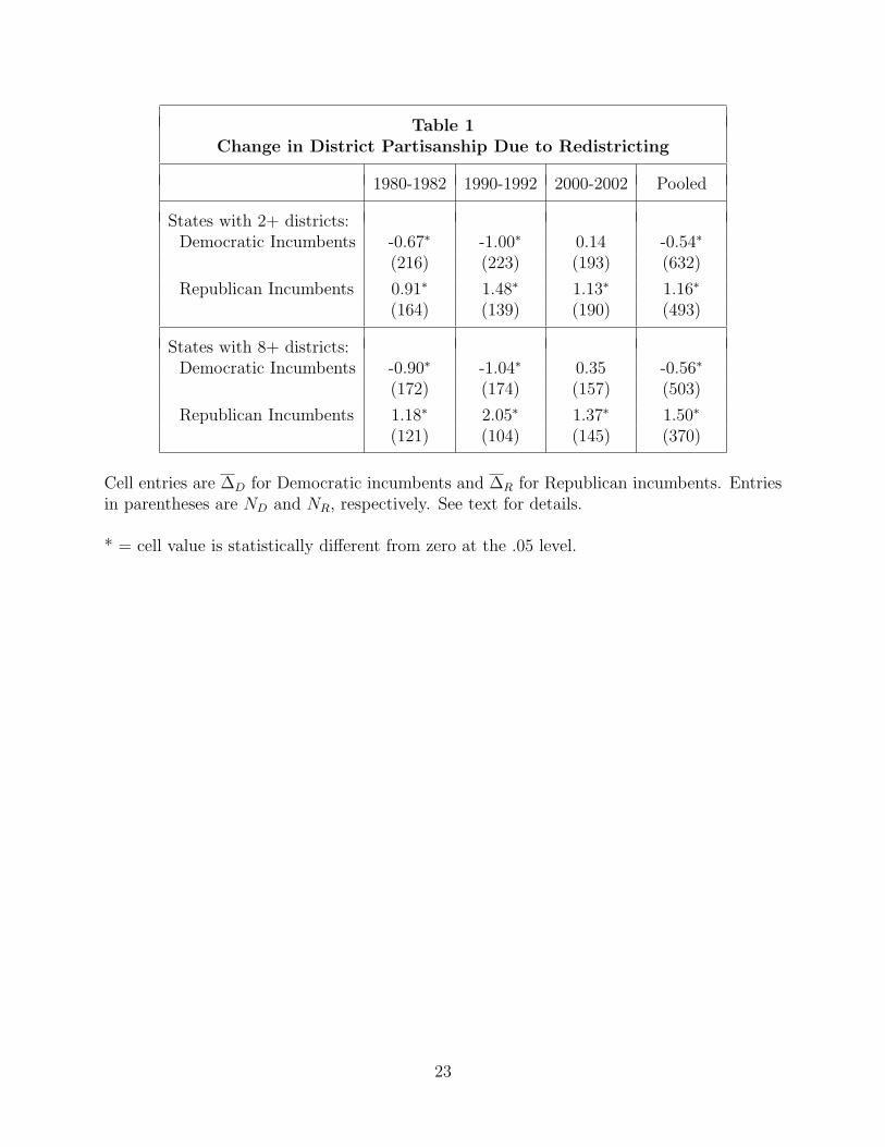
Table 1Change in District Partisanship Due to Redistricting
1980-1982 1990-1992 2000-2002 Pooled
States with 2+ districts:Democratic Incumbents -0.67∗ -1.00∗ 0.14 -0.54∗
(216) (223) (193) (632)
Republican Incumbents 0.91∗ 1.48∗ 1.13∗ 1.16∗
(164) (139) (190) (493)
States with 8+ districts:Democratic Incumbents -0.90∗ -1.04∗ 0.35 -0.56∗
(172) (174) (157) (503)
Republican Incumbents 1.18∗ 2.05∗ 1.37∗ 1.50∗
(121) (104) (145) (370)
Cell entries are ∆D for Democratic incumbents and ∆R for Republican incumbents. Entriesin parentheses are ND and NR, respectively. See text for details.
* = cell value is statistically different from zero at the .05 level.
23
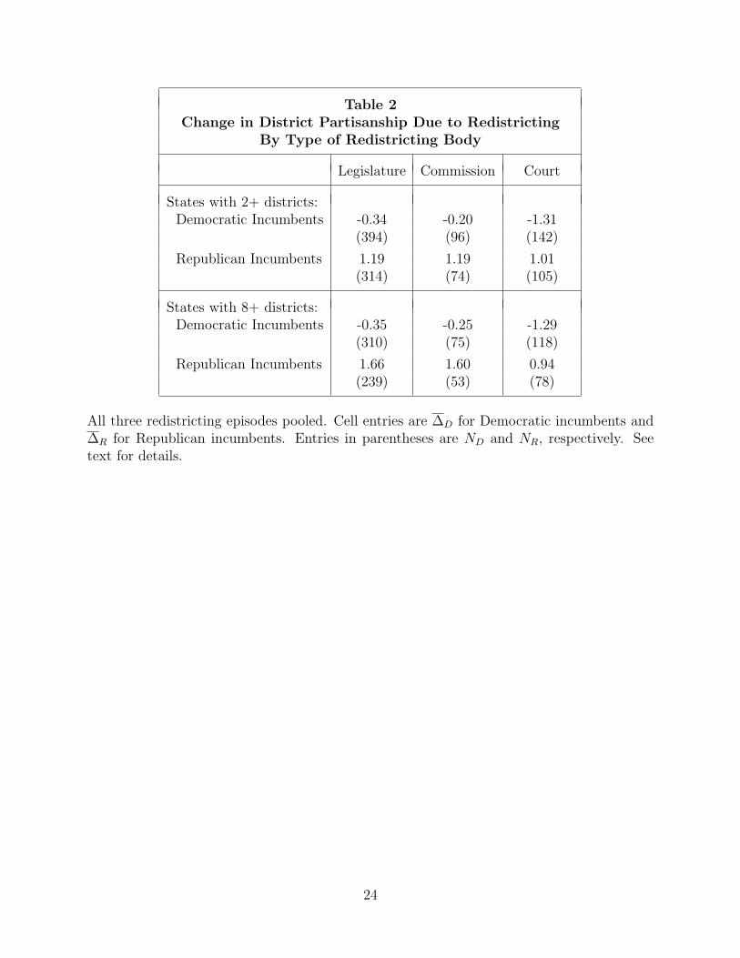
Table 2Change in District Partisanship Due to Redistricting
By Type of Redistricting Body
Legislature Commission Court
States with 2+ districts:Democratic Incumbents -0.34 -0.20 -1.31
(394) (96) (142)
Republican Incumbents 1.19 1.19 1.01(314) (74) (105)
States with 8+ districts:Democratic Incumbents -0.35 -0.25 -1.29
(310) (75) (118)
Republican Incumbents 1.66 1.60 0.94(239) (53) (78)
All three redistricting episodes pooled. Cell entries are ∆D for Democratic incumbents and∆R for Republican incumbents. Entries in parentheses are ND and NR, respectively. Seetext for details.
24
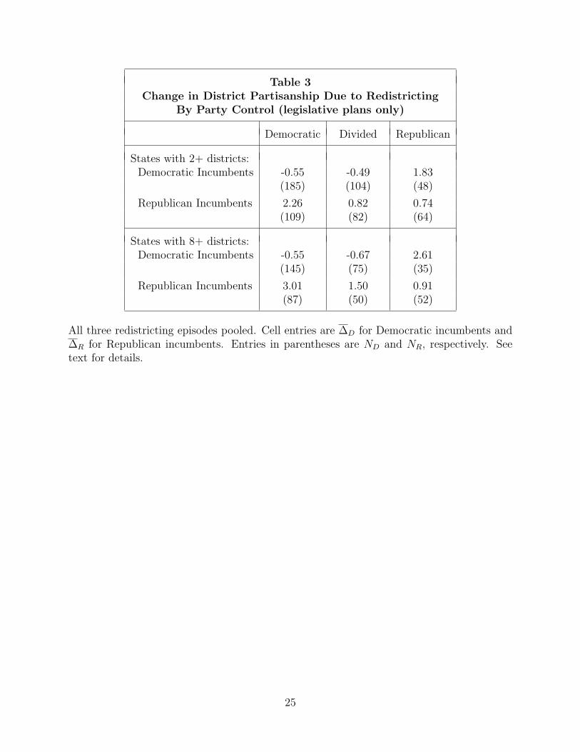
Table 3Change in District Partisanship Due to Redistricting
By Party Control (legislative plans only)
Democratic Divided Republican
States with 2+ districts:Democratic Incumbents -0.55 -0.49 1.83
(185) (104) (48)
Republican Incumbents 2.26 0.82 0.74(109) (82) (64)
States with 8+ districts:Democratic Incumbents -0.55 -0.67 2.61
(145) (75) (35)
Republican Incumbents 3.01 1.50 0.91(87) (50) (52)
All three redistricting episodes pooled. Cell entries are ∆D for Democratic incumbents and∆R for Republican incumbents. Entries in parentheses are ND and NR, respectively. Seetext for details.
25
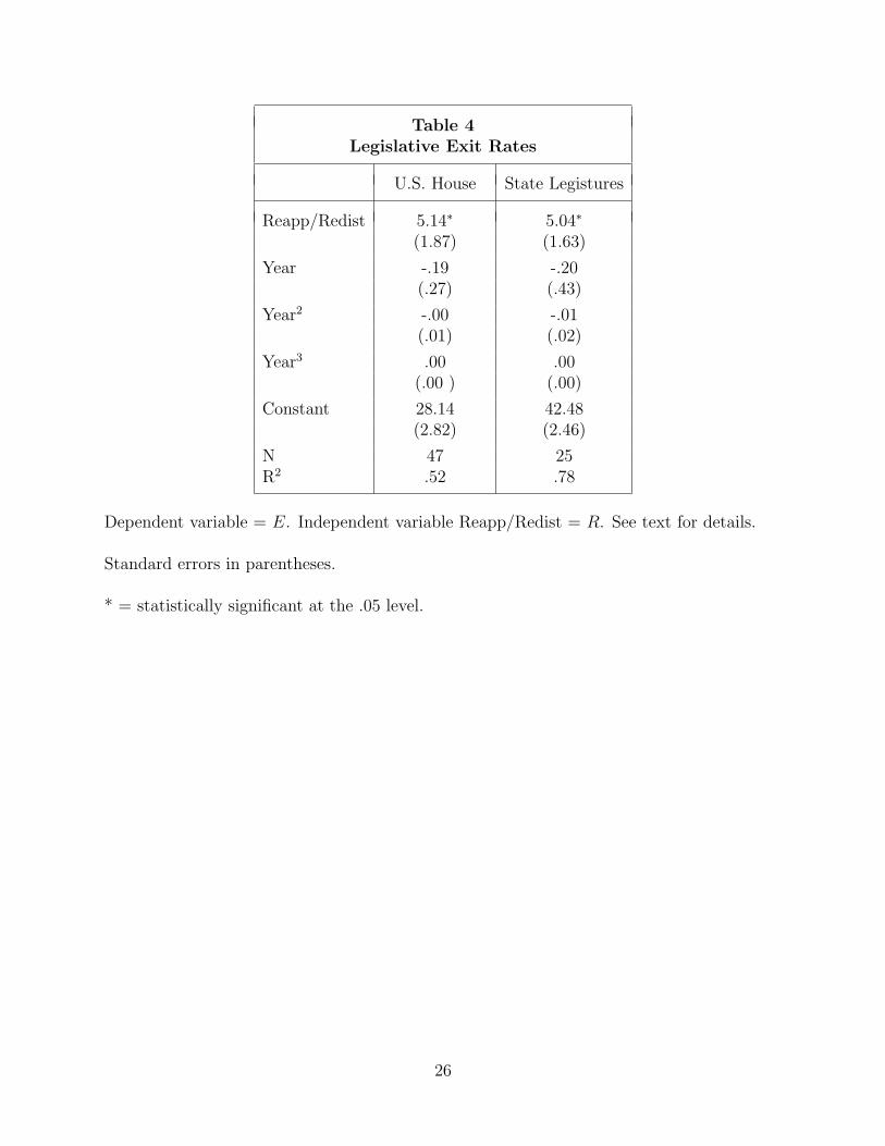
Table 4Legislative Exit Rates
U.S. House State Legistures
Reapp/Redist 5.14∗ 5.04∗
(1.87) (1.63)
Year -.19 -.20(.27) (.43)
Year2 -.00 -.01(.01) (.02)
Year3 .00 .00(.00 ) (.00)
Constant 28.14 42.48(2.82) (2.46)
N 47 25R2 .52 .78
Dependent variable = E. Independent variable Reapp/Redist = R. See text for details.
Standard errors in parentheses.
* = statistically significant at the .05 level.
26
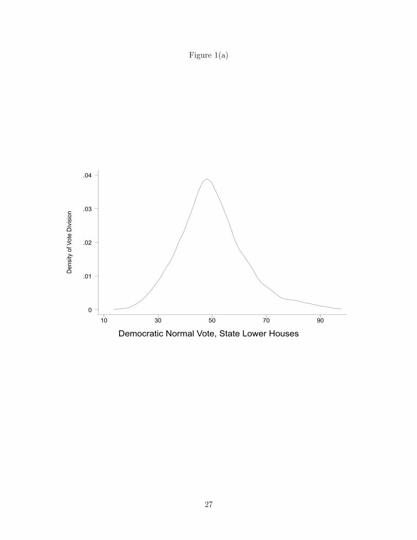
Figure 1(a)
Den
sity
of V
ote
Div
isio
n
Democratic Normal Vote, State Lower Houses
10 30 50 70 90
0
.01
.02
.03
.04
27
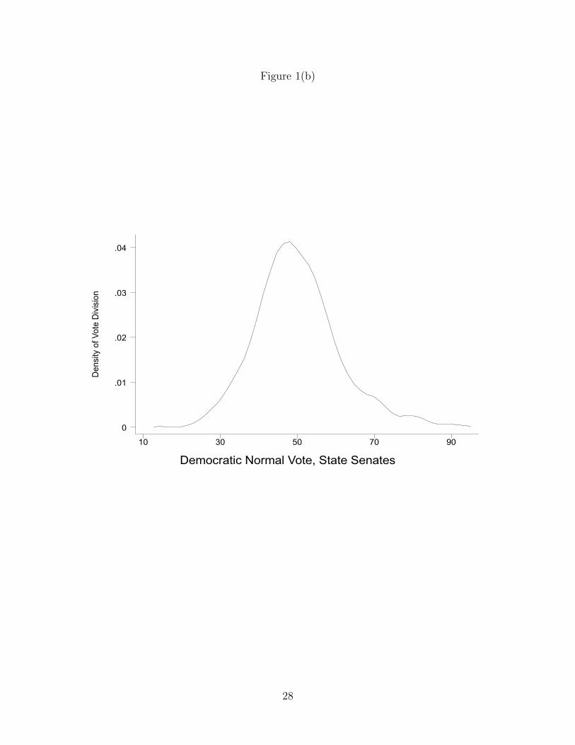
Figure 1(b)
Den
sity
of V
ote
Div
isio
n
Democratic Normal Vote, State Senates
10 30 50 70 90
0
.01
.02
.03
.04
28
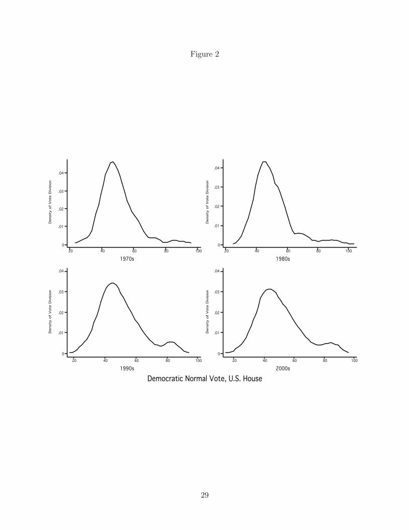
Figure 2
Democratic Normal Vote, U.S. House
Democratic Normal Vote, U.S. House
Democratic Normal Vote, U.S. HouseDensity of Vote Division
Den
sity
of
Vot
e D
ivis
ion
Density of Vote Division1970s
1970s
1970s
20
20
2040
40
4060
60
6080
80
80100
100
1000
0
0.01
.01
.01.02
.02
.02.03
.03
.03.04
.04
.04Density of Vote Division
Den
sity
of
Vot
e D
ivis
ion
Density of Vote Division1980s
1980s
1980s
20
20
2040
40
4060
60
6080
80
80100
100
1000
0
0.01
.01
.01.02
.02
.02.03
.03
.03.04
.04
.04Density of Vote Division
Den
sity
of
Vot
e D
ivis
ion
Density of Vote Division1990s
1990s
1990s
20
20
2040
40
4060
60
6080
80
80100
100
1000
0
0.01
.01
.01.02
.02
.02.03
.03
.03.04
.04
.04Density of Vote Division
Den
sity
of
Vot
e D
ivis
ion
Density of Vote Division2000s
2000s
2000s
20
20
2040
40
4060
60
6080
80
80100
100
1000
0
0.01
.01
.01.02
.02
.02.03
.03
.03.04
.04
.04
29
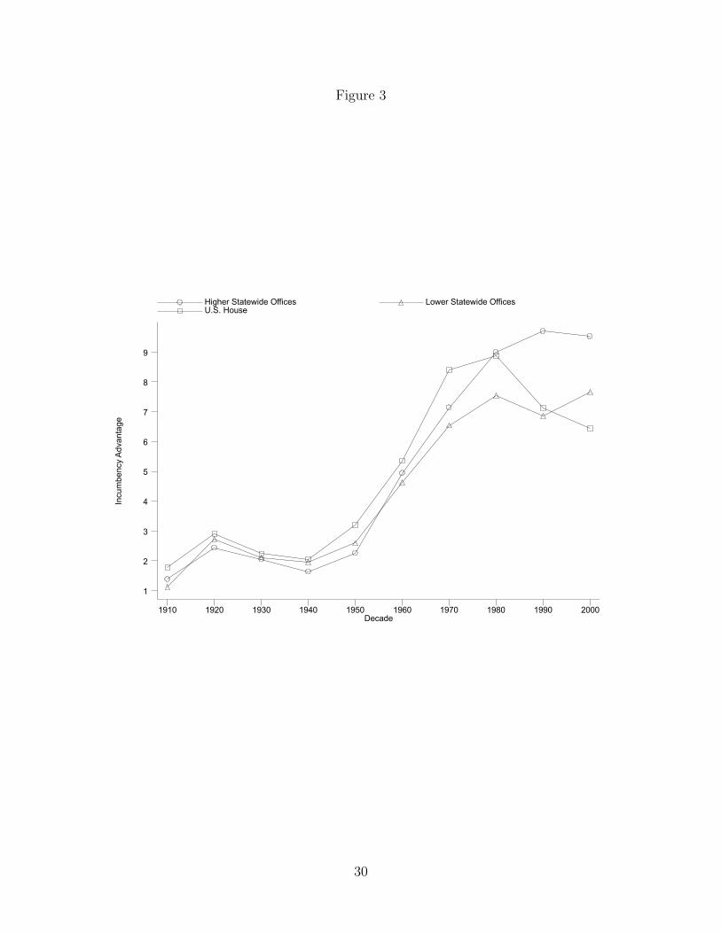
Figure 3
Incu
mbe
ncy
Ad
van
tage
Decade
Higher Statewide Offices Lower Statewide Offices U.S. House
1910 1920 1930 1940 1950 1960 1970 1980 1990 2000
1
2
3
4
5
6
7
8
9
30
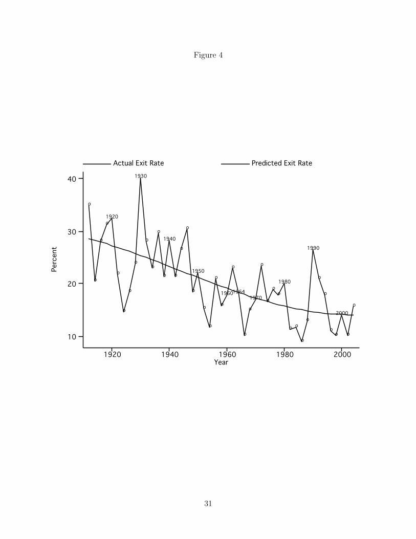
Figure 4
Percent
Perc
ent
PercentYear
Year
Year Actual Exit Rate
Actual Exit Rate Predicted Exit Rate
Predicted Exit Rate1920
1920
19201940
1940
19401960
1960
19601980
1980
19802000
2000
200010
10
1020
20
2030
30
3040
40
40o
o
oo
o
oo
o
oo
o
o1920
1920
1920o
o
oo
o
oo
o
oo
o
o1930
1930
1930o
o
oo
o
oo
o
oo
o
o1940
1940
1940o
o
oo
o
oo
o
oo
o
o1950
1950
1950o
o
oo
o
oo
o
oo
o
o1960
1960
1960o
o
o1964
1964
1964o
o
oo
o
o1970
1970
1970o
o
oo
o
oo
o
oo
o
o1980
1980
1980o
o
oo
o
oo
o
oo
o
o1990
1990
1990o
o
oo
o
oo
o
oo
o
o2000
2000
2000o
o
oo
o
o
31

Figure 5
Percent
Perc
ent
PercentYear
Year
Year Actual Exit Rate
Actual Exit Rate Predicted Exit Rate
Predicted Exit Rate1950
1950
19501960
1960
19601970
1970
19701980
1980
19801990
1990
19902000
2000
200025
25
2530
30
3035
35
3540
40
4045
45
451950
1950
1950o
o
oo
o
oo
o
oo
o
o1960
1960
1960o
o
o1964
1964
1964o
o
oo
o
o1970
1970
1970o
o
oo
o
oo
o
oo
o
o1980
1980
1980o
o
oo
o
oo
o
oo
o
o1990
1990
1990o
o
oo
o
oo
o
oo
o
o
32
Recommended