FEDERAL RESERVE BANK OF SAN FRANCISCO
WORKING PAPER SERIES
The Effects of Quasi-Random Monetary Experiments
Oscar Jorda Federal Reserve Bank of San Francisco
Moritz Schularick
University of Bonn and CEPR
Alan M. Taylor University of California, Davis
NBER, and CEPR
May 2018
Working Paper 2017-02 http://www.frbsf.org/economic-research/publications/working-papers/2017/02/
Suggested citation:
Jorda, Oscar, Moritz Schularick, Alan M. Taylor. 2018. “The Effects of Quasi-Random Monetary Experiments” Federal Reserve Bank of San Francisco Working Paper 2017-02. https://doi.org/10.24148/wp2017-02 The views in this paper are solely the responsibility of the authors and should not be interpreted as reflecting the views of the Federal Reserve Bank of San Francisco or the Board of Governors of the Federal Reserve System.
The effects of quasi-random monetary experiments?
Oscar Jorda† Moritz Schularick ‡ Alan M. Taylor §
April 2018
Abstract
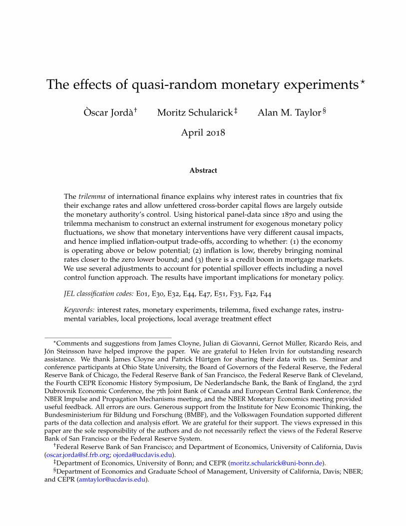
The trilemma of international finance explains why interest rates in countries that fixtheir exchange rates and allow unfettered cross-border capital flows are largely outsidethe monetary authority’s control. Using historical panel-data since 1870 and using thetrilemma mechanism to construct an external instrument for exogenous monetary policyfluctuations, we show that monetary interventions have very different causal impacts,and hence implied inflation-output trade-offs, according to whether: (1) the economyis operating above or below potential; (2) inflation is low, thereby bringing nominalrates closer to the zero lower bound; and (3) there is a credit boom in mortgage markets.We use several adjustments to account for potential spillover effects including a novelcontrol function approach. The results have important implications for monetary policy.
JEL classification codes: E01, E30, E32, E44, E47, E51, F33, F42, F44
Keywords: interest rates, monetary experiments, trilemma, fixed exchange rates, instru-mental variables, local projections, local average treatment effect
?Comments and suggestions from James Cloyne, Julian di Giovanni, Gernot Muller, Ricardo Reis, andJon Steinsson have helped improve the paper. We are grateful to Helen Irvin for outstanding researchassistance. We thank James Cloyne and Patrick Hurtgen for sharing their data with us. Seminar andconference participants at Ohio State University, the Board of Governors of the Federal Reserve, the FederalReserve Bank of Chicago, the Federal Reserve Bank of San Francisco, the Federal Reserve Bank of Cleveland,the Fourth CEPR Economic History Symposium, De Nederlandsche Bank, the Bank of England, the 23rdDubrovnik Economic Conference, the 7th Joint Bank of Canada and European Central Bank Conference, theNBER Impulse and Propagation Mechanisms meeting, and the NBER Monetary Economics meeting provideduseful feedback. All errors are ours. Generous support from the Institute for New Economic Thinking, theBundesministerium fur Bildung und Forschung (BMBF), and the Volkswagen Foundation supported differentparts of the data collection and analysis effort. We are grateful for their support. The views expressed in thispaper are the sole responsibility of the authors and do not necessarily reflect the views of the Federal ReserveBank of San Francisco or the Federal Reserve System.
†Federal Reserve Bank of San Francisco; and Department of Economics, University of California, Davis([email protected]; [email protected]).
‡Department of Economics, University of Bonn; and CEPR ([email protected]).§Department of Economics and Graduate School of Management, University of California, Davis; NBER;
and CEPR ([email protected]).

1. Introduction
Three features characterize the history of advanced economies in the past 20 years: (1) a dramatic
credit boom and bust; (2) unusually low and stable inflation throughout; and (3) a prolonged
period of below potential growth following the Global Financial Crisis. Given this background, we
investigate whether or not (1) periods of high credit growth make contractionary policy a more
forceful policy tool (2) monetary policy is less stimulative when inflation is low (and hence nominal
rates closer to the zero lower bound); and (3) monetary policy is more effective when the economy
is above potential. Answers to these questions have important implications for monetary policy and
for models of monetary economies.
It is largely an empirical matter to determine how useful a cyclical stabilizer monetary policy is.
However, empirical measures of the effect of interest rates on macroeconomic outcomes are fraught.
Macroeconomic aggregates and interest rates are jointly determined since monetary policy reflects
the central bank’s policy choices given the economic outlook. In the parlance of the policy-evaluation
literature (see, e.g., Rubin, 2005), any measure of the treatment effect of policy is contaminated by
confounders simultaneously correlated with the treatment assignment mechanism and the outcome.
Over time, several best-practice methods have emerged, but almost all are exclusively based on
the Post-WW2 U.S. experience. The general theme running through the literature is to control for
information that might explain the policymaker’s choices. Some of this control is explicit (along with
additional exclusion restrictions) such as the venerable literature based on vector autoregressions or
VARs (see, e.g., Christiano, Eichenbaum, and Evans, 1999). Romer and Romer (1989) infer exogenous
policy shifts from the narrative of the policy record though what may look like a surprise in the
minutes may not have been a surprise to the policymaker.
Continuing in this vein, Romer and Romer (2004), Cloyne and Hurgten (2016) and Coibion
et al. (2017) measure policy surprises by assuming that policymakers rely only on their staff’s
forecasts to choose policy. Taking a different approach, Kuttner (2001), Faust, Wright, and Swanson
(2004), Gertler and Karadi (2015), and Nakamura and Steinsson (forthcoming) instead appeal to
the efficiency of financial markets. A surprise change in policy rates inferred from high-frequency
asset price reactions in a short window may then serve as a natural proxy for exogenous policy
movements, though what surprised the market may not have surprised the policymaker.
This paper proposes a different approach based on a quasi-natural experiment. How a country
manages its exchange rate and how freely capital flows across its borders has direct implications for
its domestic interest rates, and hence for monetary policy. This is especially true for safe assets with
low liquidity and risk premiums, such as government securities and interbank credit.
Consider such assets which, though denominated in different currencies, are otherwise perfect
substitutes. Assume their currencies are credibly pegged for the duration of the investment and that
investors can freely transfer funds. Then, without exchange rate risk, arbitrage would equalize the
rates of return across all markets. Economic forces thus limit a country’s policy choices with respect
to the triad of capital mobility, exchange rates, and interest rates. The trilemma faced by policymakers
1
is that they can have control over two out of the three policies, but not all three simultaneously.
Articulating how and when the trilemma functions as a source of natural experiments in domestic
monetary policy is one of the contributions of this paper.
The general empirical validity of the trilemma, in both recent times and in distant historical
epochs, has been recognized for more than a decade: exogenous base country interest rate move-
ments spill into local interest rates for open pegs (Obstfeld, Shambaugh, and Taylor 2004, 2005;
Shambaugh 2004).1 Some important corollaries directly follow for empirical macroeconomics. A key
contribution by di Giovanni, McCrary, and von Wachter (2009) exploits the resulting identified local
monetary policy shocks to estimate impulse response functions for other macroeconomic outcome
variables of interest using standard VAR methods with instrumental variables.2
In this paper we take these ideas further. Variation in base rates can be used as a natural
experiment, but only by appropriately sorting the different channels of trilemma transmission.
We do this by extending the lessons from the policy evaluation literature and identification with
instrumental variables (IV) to a time series setting using local projections (Jorda 2005).
Instrumental variable applications using local projections (LP-IV) have recently appeared in a
variety of settings (see, e.g., Jorda, Schularick, and Taylor 2015; Ramey and Zubairy 2017; Stock and
Watson 2017). Here we expand the sample from the commonly studied post-WW2 period in the
U.S., and include now all of advanced economy macroeconomic history since 1870. Our results
are thus based on a much larger cross-sectional sample spanning over a century and are therefore
important in that they bring greater statistical power to robustly validate and generalize extant
findings based hitherto on the U.S. post-WW2 data alone.
Our main findings are easily summarized. First, using the subpopulation of open pegs, we find
evidence of considerable attenuation bias in policy responses when we estimate the responses to
monetary policy using traditional OLS selection-on-observables identification versus instrumental
variables identification. Second, we investigate the robustness of our new IV estimates for open
pegs as compared to the effects found by investigating the combined behavior of post-WW2 data
from the U.S. and U.K. using the established approaches of Romer and Romer (2004) and Cloyne
and Hurtgen (2016).
Third, we take several steps to control for spillover confounding (or failure of the exclusion
restriction), such as accounting for global business cycle effects, and working with base country
policy surprises rather than directly with interest rates. However, we go one step further. We discuss
a novel approach to assess spillover confounding using control functions (see Wooldridge 2010;
Conley, Hansen, and Rossi 2012) and by taking advantage of the subpopulations that make up our
data. Although it might appear obvious which way this bias goes, careful calculation shows that its
direction is ambiguous. Guided by economic reasoning, we place plausible bounds on this bias and
1Open pegs are countries that fix their exchange rate but allow relatively free movement of capital.2In related work, di Giovanni and Shambaugh (2008) used the trilemma to investigate post-WW2 output
volatility in fixed and floating regimes. Ilzetzki, Mendoza, and Vegh (2013) partition countries by exchangerate regime to study the impact of a fiscal policy shock. In previous work (Jorda, Schularick, and Taylor 2015),we studied the link between financial conditions, mortgage credit, and house prices.
2
show that this source of confounding, if anything, tends to reinforce our main findings.
We can also connect our empirical findings to recent theoretical developments that examine the
efficacy of monetary policy as a function of (household and/or firm) leverage. For example, Auclert
(2017) shows that the effectiveness of monetary policy depends on household balance sheet exposure
through the redistributive channels that interest rates can have. In Kaplan, Moll, and Violante (2017),
the mechanism operates via the heterogeneity in marginal propensities to consume of households
facing uninsurable income shocks in incomplete markets. Narrowing the focus, Iacioviello (2005)
and Cloyne, Ferreira, Surico (2015) argue that households’ reactions to monetary policy shocks
varies depending on variation in levels of mortgage indebtedness. We show that mortgage booms
indeed have strong effects on the policy trade-off that are consistent with this literature.
On the firm side, a venerable literature (Bernanke and Gertler 1995; Kashyap, Lamont, and Stein
1994; Kashyap and Stein 1995) has argued that credit constrained firms are more responsive to
monetary policy. More recently, Ottonello and Winberry (2017) focus on firm (credit) heterogeneity
to investigate asymmetry in the investment channel of monetary policy. In contrast to our earlier
findings on mortgage credit, we find little evidence of asymmetries related to firm-side credit
growth.
We also find—like others before us—that one source of state dependence comes from how
the economy responds to monetary policy in the boom versus the slump. Specifically, we find
that stimulating a weak economy is much harder than reining in a strong one. Yet another
source of state dependence comes from the level of inflation, however. Advanced economies have
recently struggled with a low-growth, low-inflation environment, referred to by commentators as
“lowflation.” The historical data show that monetary policy turns out to be rather ineffective in
lowflation environments, thus revealing another hitherto unexamined dimension in which monetary
policy is asymmetric. Perhaps this is not surprising as episodes where inflation is very low are
usually associated with nominal rates close to the zero lower bound, effectively limiting the available
monetary policy space.
This paper thus makes a number of contributions to monetary economics and to empirical
macroeconomics broadly speaking. On average, monetary policy has strong and long-lasting effects,
consistent with results from the recent literature. However, monetary policy effects can vary greatly
with the state of the economy, and that state may depend on a rich set of characteristics, including
the business cycle, inflation, and leverage. All of these findings matter when drafting theoretical
models of monetary economies. In terms of empirical methods, we are careful to spell out, in a
dynamic local projection framework, the crucial instrumental variable identification assumptions
and how they might be valid for some subpopulations but not for others. Moreover, we introduce
methods to provide well-reasoned bounds on potential biases coming from untestable failures of
the instrumental variables exclusion restriction. All of these new developments should provide for a
tighter link with long-standing policy evaluation methods in applied microeconomics and bring
empirical macroeconomics closer to a unified protocol for data analysis.
3
2. The trilemma of international finance:
a quasi-natural experiment
In open economies, exchange rates, capital flows, and monetary policy—and, thus, their management—
are all intertwined. The observation that countries cannot simultaneously control all three of these
policy components is known as the trilemma of international finance (see, e.g., Obstfeld and Taylor
1998, 2004; Obstfeld, Shambaugh, and Taylor 2004, 2005; Shambaugh 2004).
Due to the trilemma, there are situations where external conditions can generate exogenous
fluctuations in monetary policy. Inspired by this observation, at times the literature has used
short-term or central bank interest rates from major center economies as either exogenous shocks or
as instruments for domestic interest rates in noncenter countries. To take an example, di Giovanni,
McCrary, and von Wachter (2009) estimate the effect of monetary policy for twelve noncenter
European countries in the ERM system with a VAR and by using German center-country rates as an
instrument in an era of capital mobility and pegged exchange rates.
Here, due to the broader and richer historical context we study, we must separately consider
each of the three components of the trilemma to construct our instrument: (1) the choice of exchange
rate regime; (2) the degree of capital mobility; and (3) the interest rate of the base country. Moreover,
rather than directly using the base country interest rate, we first sterilize the predictable component
that could be explained by economic conditions in the base country. The specific construction of the
resulting instrumental variable, and the manner in which the analysis is designed around it, sets
our paper apart from the literature.
An international dimension is obviously critical for our analysis. So is having a long time series
to observe variation of the trilemma policy components over time. Our analysis therefore relies on
our previous work (Jorda, Schularick, and Taylor 2017). In particular, the data that we use covers
real and financial data for 17 advanced economies at annual frequency from 1870 to 2013.3 Unlike
the majority of empirical papers in monetary economics, which tend to rely on post-WW2 U.S. data,
our analysis rests both on a long time dimension and a large group of countries.
2.1. Defining the base country in fixed exchange rate regimes
As the first step in constructing the instrumental variable, we note that the trilemma naturally
breaks the data down into the three subpopulations. First, there is the group of base countries whose
currency serves as the focal anchor for pegging economies. The latter, the group denoted the pegs,
then form the second of our subpopulations. The remaining economies, which allow their currency
to be determined freely in the market, is the group we call the floats, the third subpopulation. This
subsection discusses the construction of the base subpopulation.
3These are: Australia, Belgium, Canada, Denmark, Finland, France, Germany, Italy, Japan, Netherlands,Norway, Portugal, Spain, Sweden, Switzerland, U.K. and U.S. The data and detailed descriptions are availableat http://www.macrohistory.net/data.
4
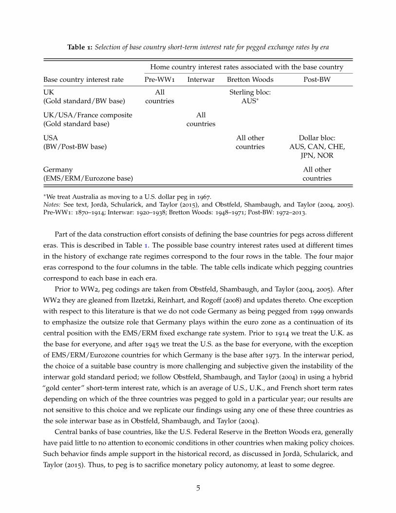
Table 1: Selection of base country short-term interest rate for pegged exchange rates by era
Home country interest rates associated with the base country
Base country interest rate Pre-WW1 Interwar Bretton Woods Post-BW
UK All Sterling bloc:(Gold standard/BW base) countries AUS∗
UK/USA/France composite All(Gold standard base) countries
USA All other Dollar bloc:(BW/Post-BW base) countries AUS, CAN, CHE,
JPN, NOR
Germany All other(EMS/ERM/Eurozone base) countries
∗We treat Australia as moving to a U.S. dollar peg in 1967.Notes: See text, Jorda, Schularick, and Taylor (2015), and Obstfeld, Shambaugh, and Taylor (2004, 2005).Pre-WW1: 1870–1914; Interwar: 1920–1938; Bretton Woods: 1948–1971; Post-BW: 1972–2013.
Part of the data construction effort consists of defining the base countries for pegs across different
eras. This is described in Table 1. The possible base country interest rates used at different times
in the history of exchange rate regimes correspond to the four rows in the table. The four major
eras correspond to the four columns in the table. The table cells indicate which pegging countries
correspond to each base in each era.
Prior to WW2, peg codings are taken from Obstfeld, Shambaugh, and Taylor (2004, 2005). After
WW2 they are gleaned from Ilzetzki, Reinhart, and Rogoff (2008) and updates thereto. One exception
with respect to this literature is that we do not code Germany as being pegged from 1999 onwards
to emphasize the outsize role that Germany plays within the euro zone as a continuation of its
central position with the EMS/ERM fixed exchange rate system. Prior to 1914 we treat the U.K. as
the base for everyone, and after 1945 we treat the U.S. as the base for everyone, with the exception
of EMS/ERM/Eurozone countries for which Germany is the base after 1973. In the interwar period,
the choice of a suitable base country is more challenging and subjective given the instability of the
interwar gold standard period; we follow Obstfeld, Shambaugh, and Taylor (2004) in using a hybrid
“gold center” short-term interest rate, which is an average of U.S., U.K., and French short term rates
depending on which of the three countries was pegged to gold in a particular year; our results are
not sensitive to this choice and we replicate our findings using any one of these three countries as
the sole interwar base as in Obstfeld, Shambaugh, and Taylor (2004).
Central banks of base countries, like the U.S. Federal Reserve in the Bretton Woods era, generally
have paid little to no attention to economic conditions in other countries when making policy choices.
Such behavior finds ample support in the historical record, as discussed in Jorda, Schularick, and
Taylor (2015). Thus, to peg is to sacrifice monetary policy autonomy, at least to some degree.
5
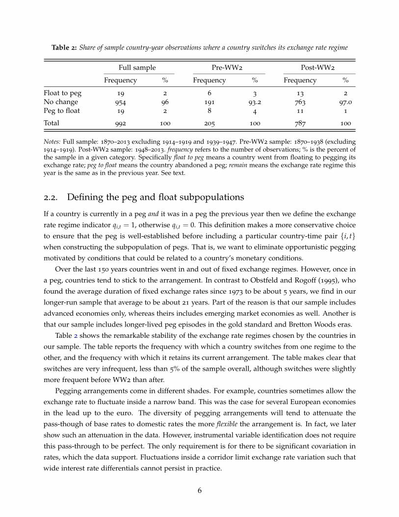
Table 2: Share of sample country-year observations where a country switches its exchange rate regime
Full sample Pre-WW2 Post-WW2
Frequency % Frequency % Frequency %
Float to peg 19 2 6 3 13 2
No change 954 96 191 93.2 763 97.0Peg to float 19 2 8 4 11 1
Total 992 100 205 100 787 100
Notes: Full sample: 1870–2013 excluding 1914–1919 and 1939–1947. Pre-WW2 sample: 1870–1938 (excluding1914–1919). Post-WW2 sample: 1948–2013. frequency refers to the number of observations; % is the percent ofthe sample in a given category. Specifically float to peg means a country went from floating to pegging itsexchange rate; peg to float means the country abandoned a peg; remain means the exchange rate regime thisyear is the same as in the previous year. See text.
2.2. Defining the peg and float subpopulations
If a country is currently in a peg and it was in a peg the previous year then we define the exchange
rate regime indicator qi,t = 1, otherwise qi,t = 0. This definition makes a more conservative choice
to ensure that the peg is well-established before including a particular country-time pair {i, t}when constructing the subpopulation of pegs. That is, we want to eliminate opportunistic pegging
motivated by conditions that could be related to a country’s monetary conditions.
Over the last 150 years countries went in and out of fixed exchange regimes. However, once in
a peg, countries tend to stick to the arrangement. In contrast to Obstfeld and Rogoff (1995), who
found the average duration of fixed exchange rates since 1973 to be about 5 years, we find in our
longer-run sample that average to be about 21 years. Part of the reason is that our sample includes
advanced economies only, whereas theirs includes emerging market economies as well. Another is
that our sample includes longer-lived peg episodes in the gold standard and Bretton Woods eras.
Table 2 shows the remarkable stability of the exchange rate regimes chosen by the countries in
our sample. The table reports the frequency with which a country switches from one regime to the
other, and the frequency with which it retains its current arrangement. The table makes clear that
switches are very infrequent, less than 5% of the sample overall, although switches were slightly
more frequent before WW2 than after.
Pegging arrangements come in different shades. For example, countries sometimes allow the
exchange rate to fluctuate inside a narrow band. This was the case for several European economies
in the lead up to the euro. The diversity of pegging arrangements will tend to attenuate the
pass-though of base rates to domestic rates the more flexible the arrangement is. In fact, we later
show such an attenuation in the data. However, instrumental variable identification does not require
this pass-through to be perfect. The only requirement is for there to be significant covariation in
rates, which the data support. Fluctuations inside a corridor limit exchange rate variation such that
wide interest rate differentials cannot persist in practice.
6
2.3. Constructing the instrument: the first stage
We have nearly all the elements in place to construct our instrumental variable. Specifically, let ∆ri,t
denote the change in short-term nominal interest rates in country i at time t, and let ∆rb(i,t),t denote
the short-term nominal interest in country i’s base country B at time t, which can differ across i and
over time—hence the notation b(i, t). Both ∆ri,t, and ∆rb(i,t),t are three-month short-term government
bill or private market interest rates, the closest measure of monetary conditions that we were able to
obtain consistently for our long and wide panel of historical data.4
Next, define the variable ki,t ∈ [0, 1] which indicates whether country i is open to international
markets or not. We base this capital mobility indicator on the index (from 0 to 100) in Quinn,
Schindler, and Toyoda (2011). We use a continuous version of their index rescaled to the unit
interval, with 0 meaning fully closed and 1 fully open. Over time, in the advanced economies
we study, full international capital mobility has been notably interrupted by the two world wars.
Resumption of mobility was nearly immediate after WW1. It was not so after WW2, in large part
due to the tight constraints on capital movements that were central to the Bretton Woods regime.
Nowadays, capital mobility is commonplace in all advanced economies.
More specifically, we find that in our data the average value of k for the pegs in the full sample
is 0.87 (with a standard deviation of 0.21) versus 0.70 (0.31) for floats. In the post-WW2 era, these
averages are virtually indistinguishable from one another, with values of 0.76 (0.24) for pegs and
0.74 (0.30) for floats. Thus, it cannot be said that pegs on average used more restrictions on capital to
regain control over monetary policy than floats, and the subsamples are balanced on this dimension.
Moreover, note that it is clear that restrictions on capital mobility have not been used as a high-
frequency policy tool by pegging economies since the index is very slow moving, unlike interest
rate policy settings.
Finally, we denote with ∆rb(i,t),t movements in base country b(i, t) rates explained by observable
controls for that base country, denoted xb(i,t),t. Similarly, denote with xi,t a broad set of domestic
macroeconomic controls in country i at time t. Such controls include current and lagged values of
macroeconomic aggregates, and lagged values of the policy variable. Putting all these elements
together, our instrument is constructed to equal zi,t ≡ ki,t (∆rb(i,t),t − ∆rb(i,t),t) if qi,t = 1, and to equal
zi,t = 0 if qi,t = 0.
Notice three features of how the instrument is constructed. First is our focus on isolating
unpredictable movements in base country interest rates rather than base rates themselves. The idea
is to narrow the focus to movements in base country rates that would not have been predicted
using observable information by country i.5 Moreover, the extent to which there are external
factors affecting base and pegging economies will tend to contaminate the raw measure but not its
4Swanson and Williams (2014) and Gertler and Karadi (2015) are two recent examples of papers that stepback from using typical interbank overnight rates and instead measure monetary policy with governmentrates for bonds at a duration of up to 2-years in some cases.
5A lower standard of proof would be to use ∆rb(i,t),t directly. Experiments with such an instrumentproduced similar results to those reported below and are available upon request.
7
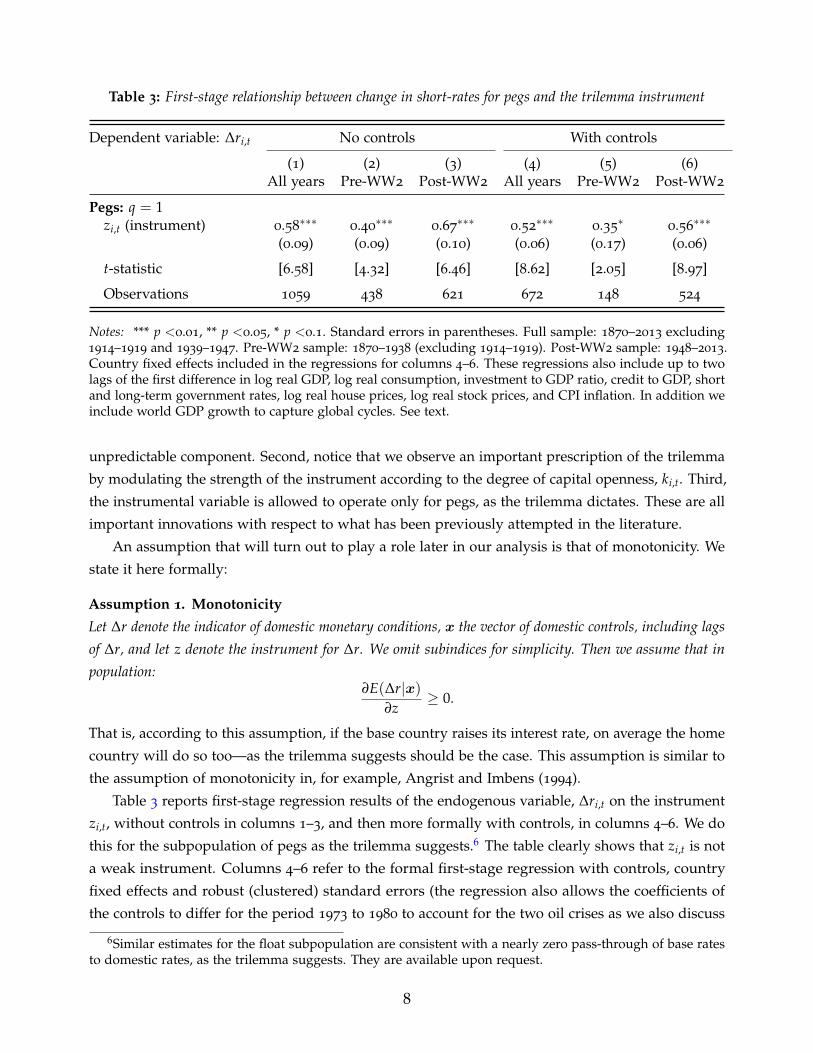
Table 3: First-stage relationship between change in short-rates for pegs and the trilemma instrument
Dependent variable: ∆ri,t No controls With controls
(1) (2) (3) (4) (5) (6)All years Pre-WW2 Post-WW2 All years Pre-WW2 Post-WW2
Pegs: q = 1zi,t (instrument) 0.58
∗∗∗0.40
∗∗∗0.67
∗∗∗0.52
∗∗∗0.35
∗0.56
∗∗∗
(0.09) (0.09) (0.10) (0.06) (0.17) (0.06)
t-statistic [6.58] [4.32] [6.46] [8.62] [2.05] [8.97]
Observations 1059 438 621 672 148 524
Notes: *** p <0.01, ** p <0.05, * p <0.1. Standard errors in parentheses. Full sample: 1870–2013 excluding1914–1919 and 1939–1947. Pre-WW2 sample: 1870–1938 (excluding 1914–1919). Post-WW2 sample: 1948–2013.Country fixed effects included in the regressions for columns 4–6. These regressions also include up to twolags of the first difference in log real GDP, log real consumption, investment to GDP ratio, credit to GDP, shortand long-term government rates, log real house prices, log real stock prices, and CPI inflation. In addition weinclude world GDP growth to capture global cycles. See text.
unpredictable component. Second, notice that we observe an important prescription of the trilemma
by modulating the strength of the instrument according to the degree of capital openness, ki,t. Third,
the instrumental variable is allowed to operate only for pegs, as the trilemma dictates. These are all
important innovations with respect to what has been previously attempted in the literature.
An assumption that will turn out to play a role later in our analysis is that of monotonicity. We
state it here formally:
Assumption 1. Monotonicity
Let ∆r denote the indicator of domestic monetary conditions, x the vector of domestic controls, including lagsof ∆r, and let z denote the instrument for ∆r. We omit subindices for simplicity. Then we assume that inpopulation:
∂E(∆r|x)∂z
≥ 0.
That is, according to this assumption, if the base country raises its interest rate, on average the home
country will do so too—as the trilemma suggests should be the case. This assumption is similar to
the assumption of monotonicity in, for example, Angrist and Imbens (1994).
Table 3 reports first-stage regression results of the endogenous variable, ∆ri,t on the instrument
zi,t, without controls in columns 1–3, and then more formally with controls, in columns 4–6. We do
this for the subpopulation of pegs as the trilemma suggests.6 The table clearly shows that zi,t is not
a weak instrument. Columns 4–6 refer to the formal first-stage regression with controls, country
fixed effects and robust (clustered) standard errors (the regression also allows the coefficients of
the controls to differ for the period 1973 to 1980 to account for the two oil crises as we also discuss
6Similar estimates for the float subpopulation are consistent with a nearly zero pass-through of base ratesto domestic rates, as the trilemma suggests. They are available upon request.
8
below). The t-statistic on zi,t is well above 3 for the full and post-WW2 samples. Moreover, notice
that the slope estimates in columns 4–6 are similar to those in columns 1–3, which suggests that the
instrument is relevant in that contains information that is quite different from that contained in the
controls.7
3. Methods
The central goal of our paper is to evaluate the effects of a domestic monetary policy intervention
on domestic macroeconomic outcomes. Identification of the causal effect is based on an external
instrumental variables (IV) approach using the trilemma discussed in the previous section. Identifi-
cation depends on the exclusion restriction, in this case the assumption that base country interest
rates affect peg economies only through the interest rate channel.
When the model is just identified—as ours is—the exclusion restriction is untestable. Based on
how the instrument is constructed and the economics of the trilemma, we have solid justification
for why the exclusion restriction holds, at least approximately. However, we also discuss a method
to provide interpretable bounds on spillover effects even if the exclusion restriction were to fail—
another innovation of this paper relative to the literature.
We calculate these bounds by taking advantage of the float subpopulation for which the trilemma
instrument is known to be invalid. The way we go about calculating such bounds it to assume
the worst case scenario, that is, that any effect of base country interest rates on floating economies
operates entirely through spillover effects and not through interest rate channels. We show how
an estimate of this worst-case scenario spillover effect in the floats can be used to then calculate a
bound for the IV estimates in the peg subpopulation, as we shall explain momentarily.
We can begin by defining the random variable y(h) in reference to a macroeconomic out-
come of interest observed h periods from today for h = 0, 1, . . . , H − 1. For example, we may
be interested in the growth rate approximation given by 100 times the log difference between
real GDP in t + h relative to t when computing a cumulative impulse response resulting from
a monetary policy intervention. We can collect all such random variables into an H × 1 vector
y = (y(0), y(1), . . . , y(h), . . . , y(H − 1)).
In reporting the average effects of a policy intervention over time, we will adopt the convention
of normalizing the intervention to a 1 percentage point (100 bps) increase in interest rates (∆r = 1)
compared to a counterfactual of leaving interest rates unchanged (∆r = 0). Further, we denote as
x the vector of controls which include lags of the outcome, lags of the intervention variable, and
any other exogenous or predetermined variables. Moreover, we assume that the controls affect the
outcome linearly for the moment.
7The control list includes up to two lags of the first difference in log real GDP, log real consumption,investment to GDP ratio, credit to GDP, short and long-term government rates, log real house prices, log realstock prices, and CPI inflation.
9
Like the average treatment effect in applied microeconomics, we are interested in the impulse
response given by the forecast path for the outcome variable and its counterfactual, that is:
RATE ≡ E(y|∆r = 1; x)− E(y|∆r = 0; x) (1)
where we note that RATE is a vector of dimension H × 1. Notice that RATE could be estimated by
using a vector autoregression (or VAR). For reasons that will become apparent shortly, we prefer to
approximate the conditional expectations in (1) using local projections (Jorda, 2005). In particular,
consider the following set of panel local projections:
yi,t+h = αi,h + ∆ri,tβh + xi,tγh + νi,t+h ; for h = 0, . . . , H − 1, (2)
using a longitudinal sample where i = 1, . . . , N; and t = 1, . . . , T. Expression (2) could be naıvely
estimated by standard OLS panel-data methods, and we will refer such an estimate as LP-OLS.
Notice that αi,h is a fixed effect. We also note for later reference that we will include a global GDP
variable to parsimoniously remove global business cycle effects. From this regression it is easy to
see that RATE = β = (β0, . . . , βH−1)′.
What about causality? Under OLS, the identification of causal effects for the coefficient βh in
expression (2) relies, roughly speaking, on ∆r being randomly assigned given the controls included
in the regression. One way to express the conditions under which such a regression would be
causally interpretable is to use the potential outcomes approach (see Rubin, 1974). Using standard
notation, and in a linear setup such as ours, it would suffice to assume the following:
Assumption 2. Conditional mean independence
Let y1 denote the random variable drawn from the distribution of potential outcomes when ∆r = 1—thetreated subpopulation. Similarly, let y0 refer to potential outcomes from the control subpopulation, that is,when ∆r = 0. We assume that:
E(y1|∆r = 1, x) = E(y1|x) and E(y0|∆r = 0, x) = E(y0|x) , (3)
that is, conditional on the controls, x, there is no selection mechanism that explains differences in theconditional means of the potential outcomes y1 and y0.
Put differently, given x, ∆r is as good as if it were randomly assigned. Parenthetically, this type of
assumption permeates the VAR literature, although it is rarely stated like this. For example, identifi-
cation based on zero short-run restrictions and Cholesky ordering is a type of conditional mean
assumption. The Cholesky ordering is equivalent to calculating the conditional mean E(y|∆r, x)
by including in the control vector x those variables ordered first in the assumed ordering dated
contemporaneously with the treatment variable ∆r in addition to their lags. However, as we show
below, the data strongly reject this conditional mean assumption. For this reason we have to explore
other methods to achieve identification based on the trilemma instrument that we now discuss.
10
3.1. Identification with external instruments
Fluctuations in the unpredictable component of the base country policy rate, modulated according
to the mobility of arbitrage capital across borders, induce exogenous fluctuations in the policy
rate of countries that peg their exchange rate to it. This leads us to conclude that the correlation
between the trilemma instrument and the policy intervention variable can thus be used to calculate
a local impulse response in the sense of the local average treatment effect in Angrist and Imbens (1994).
However, we need to be aware that, because the instrument does not operate for floats, causal effects
can only be formally estimated for the subpopulation of pegs.
In terms of the conditions needed for our instrument to be valid, we make the usual assumptions,
that is:
Assumption 3. Relevance and exogeneity
L(∆r|x, z; q = 1) 6= L(∆|x; q = 1) relevance
L(yj|x, ∆r, z; q = 1) = L(yj|x, ∆r; q = 1) for j = 0, 1 exogeneity (4)
where, for example, L(∆r|x, z) refers to the linear projection of ∆r on x and z.
A few comments are in order. First, we see that Assumption 3 is milder than making assumptions
on conditional expectations since identification is based on the usual covariance between instrument
and policy intervention. Note also that we explicitly condition only on q = 1 to emphasize that
in our trilemma-based application, these assumptions only need to hold for the subpopulation of
pegs. And we remark again that one of the robustness checks that we introduce below will allow for
failure of the exclusion restriction in expression (4).
We now have the ingredients required to estimate the causal effects of a policy intervention for
the subpopulation of pegs. Using Assumptions 1 and 3, and given a sample of panel data, we can
now estimate the following set of local projections using instrumental variables (LP-IV):
yi,t+h = αi,h + xi,tγh + ∆ri,tβh + νi,t+h ; for h = 0, . . . , H − 1 , (5)
which can be compared to the LP-OLS form at (2), and where the estimates of ∆ri,t come from the
first stage regression:
∆ri,t = ai + xi,tg + zi,tb + ηi,t. (6)
The impulse response can therefore be expressed as:
RLATE = E(y1 − y0|∆r, x, z; q = 1) = β = (β0, . . . , βH−1)′ (7)
which can be estimated from the sequence of equations in expression (5).
11
Several remarks are worth making. First, the control vector x will include contemporaneous
values of all the variables except the outcome variable (since we begin at h = 0 to avoid singularity).
This is to provide insurance against variation in the policy intervention that could have been
explained by information observed concurrently with the policy treatment. Second, expressions (5)
and (6) include fixed effects and global GDP to capture global business cycle effects. Third, standard
errors are estimated using a clustered-robust covariance matrix estimator. This option allows for
a completely unrestricted specification of the covariance matrix of the residuals in the time series
dimension by taking advantage of the cross-section. This conveniently takes care of serial correlation
in the residuals induced by the local projection setup.
3.2. Checking for spillovers: robustness of the exclusion restriction
Economically speaking, a violation of the exclusion restriction could occur if base rates affect home
outcomes through channels other than movements in home rates. Additional influences via such
channels are sometimes referred to as spillover effects. These could occur if base rates proxy for
factors common to all countries. That said, these factors would have to persist despite having
included global GDP to soak up such business cycle variation. Our problem, specifically the break
down into different subpopulations, offers a unique opportunity to assess such spillover effects
more formally than is customarily possible.
Consider a simple example to present the basic idea (Appendix A contains more formal deriva-
tions). Let y be a univariate outcome variable, ∆r the intervention, and z the instrument. We
abstract from the constant term, controls, state dependence, and any other complication for now.
The standard IV setup consists of the first and second stage regressions given by:
∆r = z b + η ,
y = ∆r β + z φ + ν . (8)
Typically we assume E(∆r ν) 6= 0, but E(z ν) = 0. The exclusion restriction refers to the assumption
that φ = 0. If this restriction were not to hold, it is easy to see that
β IVp−→ β +
φ
b.
This last expression is both simple and intuitive: the bias induced by the failure of the exclusion
restriction depends on both the size of the failure, φ, and the strength of the instrument, b. Weaker
instruments will tend to make the bias worse. This point was made in, for example, Conley, Hansen,
and Rossi (2011).
The float subpopulation (q = 0) contains useful information that we now exploit. Continue
to assume that E(z ν) = 0. We think this is justified since large economies (typically bases) with
monetary policy autonomy are unlikely to consider the macroeconomic outlook of smaller countries
12
(typically non-base floats) when setting rates. Hence, consider estimating (8) using OLS when q = 0.
Estimates of the intervention effect β and the spillover effect φ will be biased as long as E(∆r ν) 6= 0
and b 6= 0. However, it is easy to show (under standard regularity conditions) that the equivalent
OLS estimates of expression (8) are such that
βOLSp−→ β− θ
φOLSp−→ φ + b θ
with a bias term θ =E(∆r ν)E(z2)
E(z ∆r)2 − E(z2)E(∆r2). (9)
Expression (9) is intuitive. If E(∆r ν) > 0, then θ > 0 and the effect of domestic interest rates on
outcomes, βOLS, will be attenuated by the bias term θ. Similarly, the spillover effect, φOLS, will be
amplified by an amount b θ. This amplification will be larger the stronger the correlation between ∆rand z, as measured by the pseudo first-stage coefficient b.
Later we show in Table 5 that the difference between OLS and IV estimates suggests that there
is considerable attenuation bias in β. The implication is that simple OLS will tend to make the
spillover effect seem larger than it really is, and the interest rate response smaller than it really is.
Of course, if E(∆r ν) < 0, then θ < 0, and the sign of the biases would be reversed. A priori the
direction of the bias is ambiguous, as we cautioned earlier.
Without loss of generality, suppose that β = λφ, that is, the true domestic interest rate effect on
outcomes is a scaled version of the spillover effect from the foreign interest rate. In this case,
φ(λ) =(φOLS + bβOLS)
1 + λbp−→ β(λ) . (10)
Taking λ as given, we can use a control function approach to correct our LP-IV estimates of RLATE
for biases due to potential spillover effects. Expression (8) can then be rewritten as
(y− zφ(λ)) = ∆rβ + ν + z(φ(λ)− φ(λ)) .
Moreover, the usual moment conditions imply that
E(z(y− zφ(λ))) = E(z ∆r)β + E(z ν) + E(z2(φ(λ)− φ(λ))) ,
with E(z ν) = 0 , and (φ(λ)− φ(λ))1
Np
Np
∑j
z2j
p−→ 0 ,
as long as
1Np
Np
∑j
z2j
p−→ Qz < ∞ , and N f −→ ∞ as Np −→ ∞ ,
with N f and Np denoting the sizes of the subpopulations of floats and pegs respectively.
From this, we can now present a extension of our IV estimator corrected for potential spillovereffects, where this new variant is constructed by subtracting the spillover term from the outcome
13
variable in the standard IV coefficient estimator, whereby
β(λ) ≡1
Np∑ zj(yj − zjφ(λ))
1Np
∑ zj ∆rj
p−→ β(λ) .
We assume that the sample sizes of both float and peg subpopulations tend to infinity. In practice, λ
is unknown. We proceed below by using economic arguments to provide an interval of plausible
values λ ∈ [λ, λ] over which we compute β(λ). This interval provides a sense of the sensitivity of
our benchmark LP-IV estimates of RLATE to potential spillover contamination.
3.3. The roadmap
The next sections apply the methods just described to investigate the effects of a monetary policy
intervention on a wide variety of outcomes central to monetary economics. We begin by assessing
identification. A comparison between LP-OLS and LP-IV estimates across subpopulations reveals
considerable attenutation bias from poor identification when relying on conditional mean indepen-
dence. The trilemma instrument greatly improves our estimates. Moreover, to remove any doubts
that these results are driven by spillover effects, we conduct robustness analysis. If anything, the
main results strengthen.
The next phase of our analysis explores potential state-dependence in our results. The LP-IV
framework that we espouse is then particularly well-suited to evaluate whether monetary policy
interventions are more or less effective depending on several stratifications of the data. This turns
out to be the case, with important implications for how we think about traditional monetary models.
4. Monetary policy interventions:
understanding the subpopulations
Throughout its history, a country can fall into any of the following bins defined earlier: pegs, floats,
and bases. For example, during Bretton Woods, Germany was in a peg to the dollar. With the end of
Bretton Woods, and later the introduction of the European Monetary System, we consider Germany
to become a base for many European economies. And there are other periods where we classify
Germany as a float, as was the case for much of the interwar period. Other than bases, all other
countries are either floats or pegs, depending on the period.
When presenting results, we will always measure and display the outcome variable in deviations
relative to its initial value in year 0, with units shown in percent of the initial year value (computed
as log change times 100), except in the case of interest rates where the response will be measured in
units of percentage points. The policy intervention variable will be defined as the one-year change
in the short-term interest rate in year 0, and normalized in all cases to a 1 percentage point, or 100
basis points (bps) increase.
14
The vector of explanatory variables includes a rich set of macroeconomic controls consisting
of the first-difference of the contemporaneous values of all variables (excluding the response or
outcome variable), and up to 2 lags of the first-difference of all variables, including the response
variable. The list of macroeconomic controls is: log real GDP per capita; log real real consumption
per capita; log real real investment per capita; log consumer price index; short-term interest rate
(usually a 3-month government security); long-term interest rate (usually a 5-year government
security); log real house prices; log real stock prices; and the credit to GDP ratio.8
In almost all respects, we found that this estimation setup produced stable outcomes. However,
in line with the well-known “price puzzle” literature (e.g., Eichenbaum 1992; Sims 1992; Hanson
2004), we found that there was substantial instability in the coefficients of the control variables,
and that this finding was driven by the postwar high-inflation period of the 1970s. The traditional
resolution of this puzzle has been to include commodity prices as a way to control for oil shocks.
Given the constraints of our data, we addressed this issue by allowing the controls to take on a
potentially different coefficient for the subsample period of years from 1973 to 1980 inclusive, thus
bracketing the volatile period of the two oil crises.
4.1. LP-OLS: subpopulation RATE under conditional mean independence
We begin our analysis by following the older selection-on-observables tradition. We naıvely estimate
via LP-OLS the effect of an interest rate intervention on output (measured by log real GDP per
capita) and prices (measured by log CPI)—two variables that commonly feature in many central
bank mandates. These results are provided in Table 4 and are based on a panel regression that allows
the relevant coefficient estimates to vary for each of the three subpopulations that we consider: pegs,
floats and bases.
These estimates are a natural benchmark: if regression control is sufficient to achieve identifica-
tion, then we could quite easily obtain estimates of RATE simply by averaging standard panel-based
estimates across subpopulations. Hence the table evaluates whether estimates across subpopulations
are statistically different from one another. In addition, we also provide a joint test that, over the
5 horizons considered, the effect of interest rates on output and prices is zero. The analysis is
conducted over the full and the post-WW2 samples.
Consider the output responses first, reported in columns 1–3. Full sample results indicate some
minor differences across subpopulations. The p-values of the null that the coefficients are equal is
reported in column 4. The differences are economically minor, however. The post-WW2 results in
column 4 suggest that if anything, the differences are even less important over this sample. Generally
speaking, the coefficient estimates have the expected signs. An increase in interest rates causes
output to decline. Note that in all cases the effect is statistically different from zero as reported in
the rows labeled H0 : subATE = 0, by which we denote “subpopulation ATE.”
8The data are described in more detail in Jorda, Schularick, and Taylor (2017), and its online appendix.
15
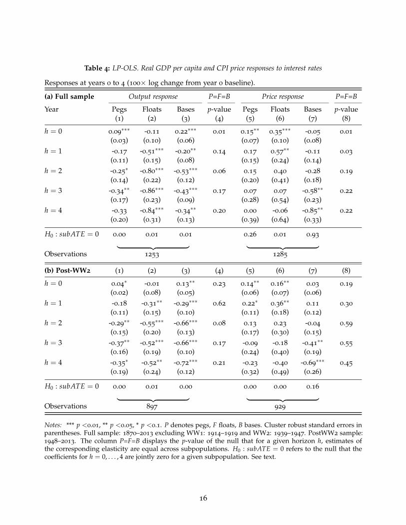
Table 4: LP-OLS. Real GDP per capita and CPI price responses to interest rates
Responses at years 0 to 4 (100× log change from year 0 baseline).
(a) Full sample Output response P=F=B Price response P=F=B
Year Pegs Floats Bases p-value Pegs Floats Bases p-value(1) (2) (3) (4) (5) (6) (7) (8)
h = 0 0.09∗∗∗ -0.11 0.22
∗∗∗0.01 0.15
∗∗0.35
∗∗∗ -0.05 0.01
(0.03) (0.10) (0.06) (0.07) (0.10) (0.08)h = 1 -0.17 -0.51
∗∗∗ -0.20∗∗
0.14 0.17 0.57∗∗ -0.11 0.03
(0.11) (0.15) (0.08) (0.15) (0.24) (0.14)h = 2 -0.25
∗ -0.80∗∗∗ -0.53
∗∗∗0.06 0.15 0.40 -0.28 0.19
(0.14) (0.22) (0.12) (0.20) (0.41) (0.18)h = 3 -0.34
∗∗ -0.86∗∗∗ -0.43
∗∗∗0.17 0.07 0.07 -0.58
∗∗0.22
(0.17) (0.23) (0.09) (0.28) (0.54) (0.23)h = 4 -0.33 -0.84
∗∗∗ -0.34∗∗
0.20 0.00 -0.06 -0.85∗∗
0.22
(0.20) (0.31) (0.13) (0.39) (0.64) (0.33)
H0 : subATE = 0 0.00 0.01 0.01 0.26 0.01 0.93︸ ︷︷ ︸ ︸ ︷︷ ︸Observations 1253 1285
(b) Post-WW2 (1) (2) (3) (4) (5) (6) (7) (8)
h = 0 0.04∗ -0.01 0.13
∗∗0.23 0.14
∗∗0.16
∗∗0.03 0.19
(0.02) (0.08) (0.05) (0.06) (0.07) (0.06)h = 1 -0.18 -0.31
∗∗ -0.29∗∗∗
0.62 0.22∗
0.36∗∗
0.11 0.30
(0.11) (0.15) (0.10) (0.11) (0.18) (0.12)h = 2 -0.29
∗∗ -0.55∗∗∗ -0.66
∗∗∗0.08 0.13 0.23 -0.04 0.59
(0.15) (0.20) (0.13) (0.17) (0.30) (0.15)h = 3 -0.37
∗∗ -0.52∗∗∗ -0.66
∗∗∗0.17 -0.09 -0.18 -0.41
∗∗0.55
(0.16) (0.19) (0.10) (0.24) (0.40) (0.19)h = 4 -0.35
∗ -0.52∗∗ -0.72
∗∗∗0.21 -0.23 -0.40 -0.69
∗∗∗0.45
(0.19) (0.24) (0.12) (0.32) (0.49) (0.26)
H0 : subATE = 0 0.00 0.01 0.00 0.00 0.00 0.16︸ ︷︷ ︸ ︸ ︷︷ ︸Observations 897 929
Notes: *** p <0.01, ** p <0.05, * p <0.1. P denotes pegs, F floats, B bases. Cluster robust standard errors inparentheses. Full sample: 1870–2013 excluding WW1: 1914–1919 and WW2: 1939–1947. PostWW2 sample:1948–2013. The column P=F=B displays the p-value of the null that for a given horizon h, estimates ofthe corresponding elasticity are equal across subpopulations. H0 : subATE = 0 refers to the null that thecoefficients for h = 0, . . . , 4 are jointly zero for a given subpopulation. See text.
16
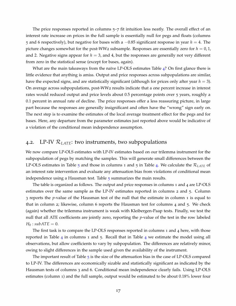
The price responses reported in columns 5–7 fit intuition less neatly. The overall effect of an
interest rate increase on prices in the full sample is essentially null for pegs and floats (columns
5 and 6 respectively), but negative for bases with a −0.85 significant response in year h = 4. The
picture changes somewhat for the post-WW2 subsample. Responses are essentially zero for h = 0, 1,
and 2. Negative signs appear for h = 3, and 4, but the responses are generally not very different
from zero in the statistical sense (except for bases, again).
What are the main takeaways from the naıve LP-OLS estimates Table 4? On first glance there is
little evidence that anything is amiss. Output and price responses across subpopulations are similar,
have the expected signs, and are statistically significant (although for prices only after year h = 3).
On average across subpopulations, post-WW2 results indicate that a one percent increase in interest
rates would reduced output and price levels about 0.5 percentage points over 5 years, roughly a
0.1 percent in annual rate of decline. The price responses offer a less reassuring picture, in large
part because the responses are generally insignificant and often have the “wrong” sign early on.
The next step is to examine the estimates of the local average treatment effect for the pegs and for
bases. Here, any departure from the parameter estimates just reported above would be indicative of
a violation of the conditional mean independence assumption.
4.2. LP-IV RLATE: two instruments, two subpopulations
We now compare LP-OLS estimates with LP-IV estimates based on our trilemma instrument for the
subpopulation of pegs by matching the samples. This will generate small differences between the
LP-OLS estimates in Table 5 and those in columns 1 and 5 in Table 4. We calculate the RLATE of
an interest rate intervention and evaluate any attenuation bias from violations of conditional mean
independence using a Hausman test. Table 5 summarizes the main results.
The table is organized as follows. The output and price responses in columns 1 and 4 are LP-OLS
estimates over the same sample as the LP-IV estimates reported in columns 2 and 5. Column
3 reports the p-value of the Hausman test of the null that the estimate in column 1 is equal to
that in column 2; likewise, column 6 reports the Hausman test for columns 4 and 5. We check
(again) whether the trilemma instrument is weak with Kleibergen-Paap tests. Finally, we test the
null that all ATE coefficients are jointly zero, reporting the p-value of the test in the row labeled
H0 : subATE = 0.
The first task is to compare the LP-OLS responses reported in columns 1 and 4 here, with those
reported in Table 4 in columns 1 and 5. Recall that in Table 4 we estimate the model using all
observations, but allow coefficients to vary by subpopulation. The differences are relatively minor,
owing to slight differences in the sample used given the availability of the instrument.
The important result of Table 5 is the size of the attenuation bias in the case of LP-OLS compared
to LP-IV. The differences are economically sizable and statistically significant as indicated by the
Hausman tests of columns 3 and 6. Conditional mean independence clearly fails. Using LP-OLS
estimates (column 1) and the full sample, output would be estimated to be about 0.18% lower four
17
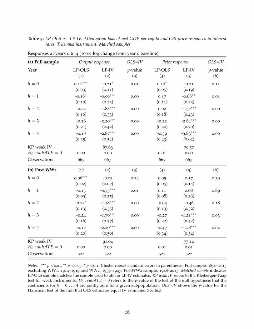
Table 5: LP-OLS vs. LP-IV. Attenuation bias of real GDP per capita and CPI price responses to interestrates. Trilemma instrument. Matched samples
Responses at years 0 to 4 (100× log change from year 0 baseline).
(a) Full sample Output response OLS=IV Price response OLS=IV
Year LP-OLS LP-IV p-value LP-OLS LP-IV p-value(1) (2) (3) (4) (5) (6)
h = 0 0.11∗∗∗ -0.21
∗0.01 0.10
∗ -0.21 0.11
(0.03) (0.11) (0.05) (0.19)h = 1 -0.18
∗ -0.99∗∗∗
0.00 0.17 -0.68∗∗
0.01
(0.10) (0.23) (0.11) (0.33)h = 2 -0.22 -1.88
∗∗∗0.00 0.02 -1.57
∗∗∗0.00
(0.16) (0.33) (0.18) (0.43)h = 3 -0.26 -2.20
∗∗∗0.00 -0.22 -2.84
∗∗∗0.00
(0.21) (0.42) (0.30) (0.70)h = 4 -0.18 -2.87
∗∗∗0.00 -0.39 -3.83
∗∗∗0.00
(0.25) (0.54) (0.43) (0.92)
KP weak IV 87.83 70.57
H0 : subATE = 0 0.00 0.00 0.01 0.00
Observations 667 667 667 667
(b) Post-WW2 (1) (2) (3) (4) (5) (6)
h = 0 0.06∗∗∗ -0.02 0.24 0.05 0.17 0.39
(0.02) (0.07) (0.05) (0.14)h = 1 -0.13 -0.75
∗∗∗0.01 0.11 0.08 0.89
(0.09) (0.25) (0.08) (0.26)h = 2 -0.22
∗ -1.58∗∗∗
0.00 -0.03 -0.46 0.18
(0.13) (0.35) (0.13) (0.32)h = 3 -0.24 -1.70
∗∗∗0.00 -0.27 -1.21
∗∗∗0.03
(0.16) (0.37) (0.22) (0.42)h = 4 -0.17 -2.20
∗∗∗0.00 -0.47 -1.78
∗∗∗0.02
(0.20) (0.50) (0.34) (0.54)
KP weak IV 91.04 77.14
H0 : subATE = 0 0.00 0.00 0.01 0.01
Observations 522 522 522 522
Notes: *** p <0.01, ** p <0.05, * p <0.1. Cluster robust standard errors in parentheses. Full sample: 1870–2013
excluding WW1: 1914–1919 and WW2: 1939–1947. PostWW2 sample: 1948–2013. Matched sample indicatesLP-OLS sample matches the sample used to obtain LP-IV estimates. KP weak IV refers to the Kleibergen-Paaptest for weak instruments. H0 : subATE = 0 refers to the p-value of the test of the null hypothesis that thecoefficients for h = 0, . . . , 4 are jointly zero for a given subpopulation. OLS=IV shows the p-value for theHausman test of the null that OLS estimates equal IV estimates. See text.
18
years after an increase in interest rates of 1%. In contrast, the LP-IV effect is measured to be nearly a
2.9% decline, or about a 0.5% annualized rate of lower growth. A similar pattern is observable for
the price response. Full sample LP-OLS estimates are largely insignificant and often have the wrong
sign. LP-IV estimates are sizable, significant, and have the right sign.
Comparing the full sample results with the post-WW2 results we find differences in the output
response to be relatively minor. The price response, however, becomes somewhat delayed or stickier
after WW2. The LP-IV response suggests that on impact and the year after, the price response is
essentially zero although by year 4, prices are expected to be about 1.8% lower than they were four
years earlier. Tests for weak instruments suggest the trilemma instrument is relevant and tests of the
null show that the RLATE estimated with LP-IV is statistically different from zero. Interest rates do
indeed have a strong causal effect on output and prices for the subpopulation of pegs.
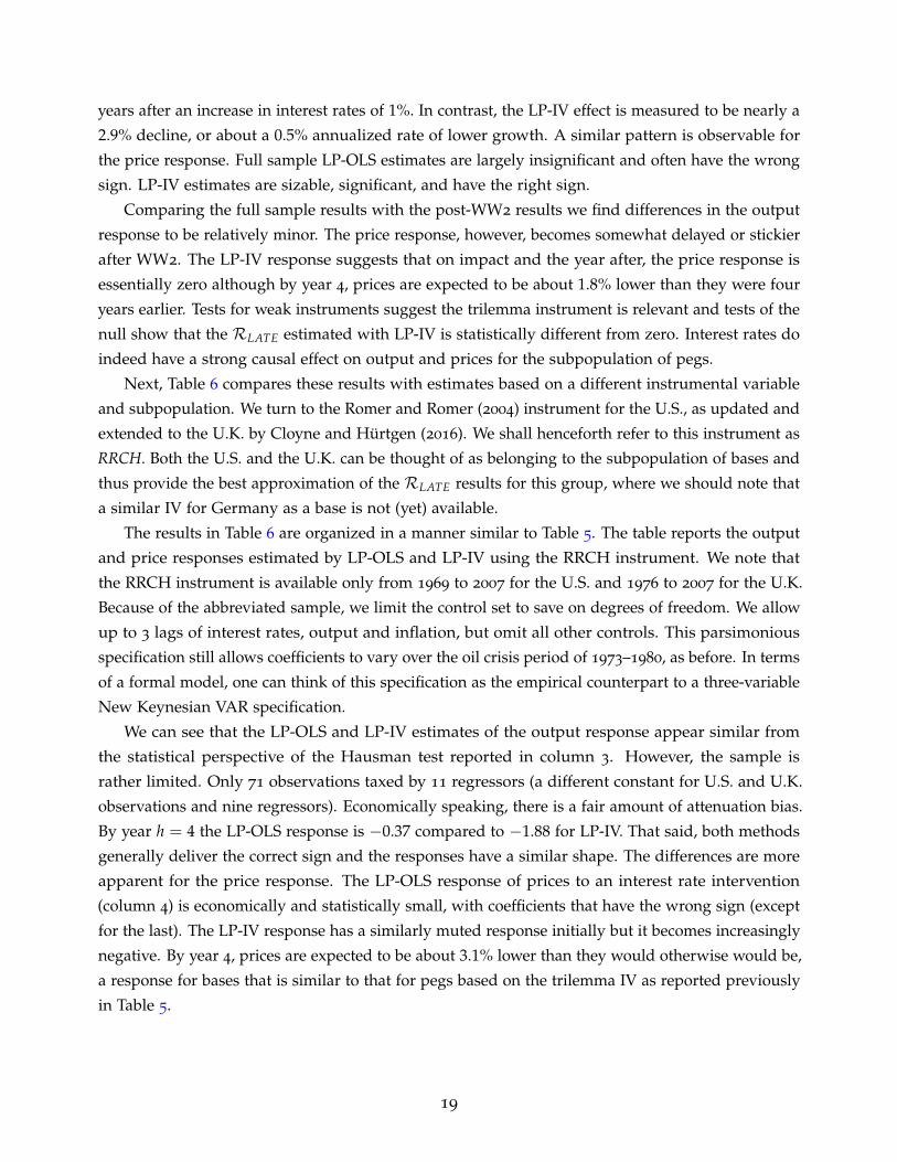
Next, Table 6 compares these results with estimates based on a different instrumental variable
and subpopulation. We turn to the Romer and Romer (2004) instrument for the U.S., as updated and
extended to the U.K. by Cloyne and Hurtgen (2016). We shall henceforth refer to this instrument as
RRCH. Both the U.S. and the U.K. can be thought of as belonging to the subpopulation of bases and
thus provide the best approximation of the RLATE results for this group, where we should note that
a similar IV for Germany as a base is not (yet) available.
The results in Table 6 are organized in a manner similar to Table 5. The table reports the output
and price responses estimated by LP-OLS and LP-IV using the RRCH instrument. We note that
the RRCH instrument is available only from 1969 to 2007 for the U.S. and 1976 to 2007 for the U.K.
Because of the abbreviated sample, we limit the control set to save on degrees of freedom. We allow
up to 3 lags of interest rates, output and inflation, but omit all other controls. This parsimonious
specification still allows coefficients to vary over the oil crisis period of 1973–1980, as before. In terms
of a formal model, one can think of this specification as the empirical counterpart to a three-variable
New Keynesian VAR specification.
We can see that the LP-OLS and LP-IV estimates of the output response appear similar from
the statistical perspective of the Hausman test reported in column 3. However, the sample is
rather limited. Only 71 observations taxed by 11 regressors (a different constant for U.S. and U.K.
observations and nine regressors). Economically speaking, there is a fair amount of attenuation bias.
By year h = 4 the LP-OLS response is −0.37 compared to −1.88 for LP-IV. That said, both methods
generally deliver the correct sign and the responses have a similar shape. The differences are more
apparent for the price response. The LP-OLS response of prices to an interest rate intervention
(column 4) is economically and statistically small, with coefficients that have the wrong sign (except
for the last). The LP-IV response has a similarly muted response initially but it becomes increasingly
negative. By year 4, prices are expected to be about 3.1% lower than they would otherwise would be,
a response for bases that is similar to that for pegs based on the trilemma IV as reported previously
in Table 5.
19
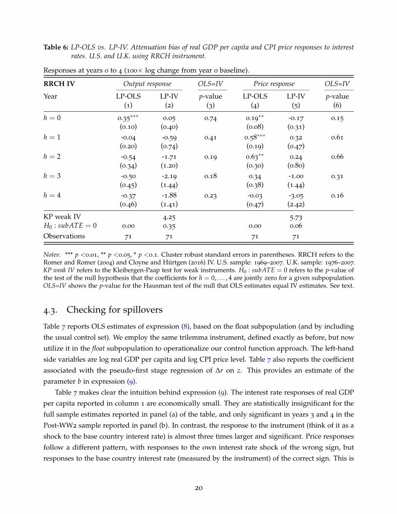
Table 6: LP-OLS vs. LP-IV. Attenuation bias of real GDP per capita and CPI price responses to interestrates. U.S. and U.K. using RRCH instrument.
Responses at years 0 to 4 (100× log change from year 0 baseline).
RRCH IV Output response OLS=IV Price response OLS=IV
Year LP-OLS LP-IV p-value LP-OLS LP-IV p-value(1) (2) (3) (4) (5) (6)
h = 0 0.35∗∗∗
0.05 0.74 0.19∗∗ -0.17 0.15
(0.10) (0.40) (0.08) (0.31)h = 1 -0.04 -0.59 0.41 0.58
∗∗∗0.32 0.61
(0.20) (0.74) (0.19) (0.47)h = 2 -0.54 -1.71 0.19 0.63
∗∗0.24 0.66
(0.34) (1.20) (0.30) (0.80)h = 3 -0.50 -2.19 0.18 0.34 -1.00 0.31
(0.45) (1.44) (0.38) (1.44)h = 4 -0.37 -1.88 0.23 -0.03 -3.05 0.16
(0.46) (1.41) (0.47) (2.42)
KP weak IV 4.25 5.73
H0 : subATE = 0 0.00 0.35 0.00 0.06
Observations 71 71 71 71
Notes: *** p <0.01, ** p <0.05, * p <0.1. Cluster robust standard errors in parentheses. RRCH refers to theRomer and Romer (2004) and Cloyne and Hurtgen (2016) IV. U.S. sample: 1969–2007. U.K. sample: 1976–2007.KP weak IV refers to the Kleibergen-Paap test for weak instruments. H0 : subATE = 0 refers to the p-value ofthe test of the null hypothesis that the coefficients for h = 0, . . . , 4 are jointly zero for a given subpopulation.OLS=IV shows the p-value for the Hausman test of the null that OLS estimates equal IV estimates. See text.
4.3. Checking for spillovers
Table 7 reports OLS estimates of expression (8), based on the float subpopulation (and by including
the usual control set). We employ the same trilemma instrument, defined exactly as before, but now
utilize it in the float subpopulation to operationalize our control function approach. The left-hand
side variables are log real GDP per capita and log CPI price level. Table 7 also reports the coefficient
associated with the pseudo-first stage regression of ∆r on z. This provides an estimate of the
parameter b in expression (9).
Table 7 makes clear the intuition behind expression (9). The interest rate responses of real GDP
per capita reported in column 1 are economically small. They are statistically insignificant for the
full sample estimates reported in panel (a) of the table, and only significant in years 3 and 4 in the
Post-WW2 sample reported in panel (b). In contrast, the response to the instrument (think of it as a
shock to the base country interest rate) is almost three times larger and significant. Price responses
follow a different pattern, with responses to the own interest rate shock of the wrong sign, but
responses to the base country interest rate (measured by the instrument) of the correct sign. This is
20
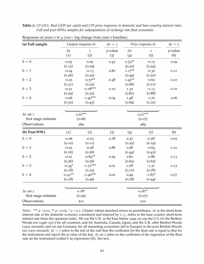
Table 7: LP-OLS. Real GDP per capita and CPI price responses to domestic and base-country interest rates.Full and post-WW2 samples for subpopulation of exchange rate float economies
Responses at years 0 to 4 (100× log change from year 0 baseline).
(a) Full sample Output response to ∆r = z Price response to ∆r = z
∆r z p-value ∆r z p-value(1) (2) (3) (4) (5) (6)
h = 0 -0.05 0.09 0.43 0.53** -0.15 0.09
(0.15) (0.09) (0.22) (0.24)h = 1 -0.24 -0.13 0.80 1.17** -0.30 0.11
(0.26) (0.22) (0.49) (0.50)h = 2 -0.23 -0.57** 0.48 1.45** -0.62 0.10
(0.31) (0.22) (0.66) (0.71)h = 3 -0.21 -1.08*** 0.10 1.35 -1.13 0.10
(0.29) (0.32) (0.80) (0.88)h = 4 -0.06 -1.40*** 0.04 1.48 -1.70 0.06
(0.30) (0.45) (0.89) (1.00)
︸ ︷︷ ︸ ︸ ︷︷ ︸∆r on z 0.20*** 0.21***
first stage estimate (0.06) (0.07)Observations 269 269
(b) Post-WW2 (1) (2) (3) (4) (5) (6)
h = 0 -0.06 -0.03 0.78 0.37 -0.36* 0.05
(0.10) (0.11) (0.22) (0.19)h = 1 -0.22 -0.28 0.86 0.58 -0.64 0.10
(0.16) (0.26) (0.44) (0.43)h = 2 -0.21 -0.84** 0.29 0.82 -0.86 0.13
(0.26) (0.36) (0.62) (0.62)h = 3 -0.34* -1.51*** 0.01 0.78 -1.31 0.13
(0.18) (0.33) (0.71) (0.78)h = 4 -0.41** -1.90*** 0.00 0.99 -1.87* 0.07
(0.18) (0.46) (0.78) (0.94)
︸ ︷︷ ︸ ︸ ︷︷ ︸∆r on z 0.18* 0.16**
first stage estimate (0.09) (0.07)Observations 210 210
Notes: *** p <0.01, ** p <0.05, * p <0.1. Cluster robust standard errors in parentheses. ∆r is the short-terminterest rate of the domestic economy considered and indexed by i; zi,t refers to the base country short-terminterest rate times the openness index. We use the U.K. as the base before 1939; we use the U.S. for the Bretton-Woods era (1946–1971) for all countries, and for Australia, Canada, Japan, and the U.K. after Bretton-Woods(1972 onward); and we use Germany for all remaining economies (all in Europe) in the post Bretton-Woodsera (1972 onward). ∆r = z refers to the test of the null that the coefficient for the float rate is equal to that forthe instrument and report the p-value of the test. ∆r on z refers to the coefficient of the regression of the floatrate on the instrument (called b in expression (8)). See text.
21
a feature we will return to in the results reported below.
Finally, we note that the regression of the domestic interest rate on the instrument and the control
set is generally non-zero, but about half to one third the magnitude of the coefficient estimated in
the first stage regression for the peg subpopulation and reported in Table 3. Compare 0.20 for the
floats with 0.40 for the pegs (using full sample estimates in the case for output). These results are
consistent with those reported in Obstfeld, Shambaugh, and Taylor (2005).
Lastly, to make any progress we need auxiliary assumptions on λ, which cannot be determined
from the data. We assert that it is natural to assume that λ ≥ 1. That is, we assume that home rates
affect outcomes at least as strongly as rates in the foreign base country. In order to provide bounds,
we use a range of values of λ between 1 and 4. In other words, the home rate effect is assumed to
be 1 to 4 times larger than the base rate effect.
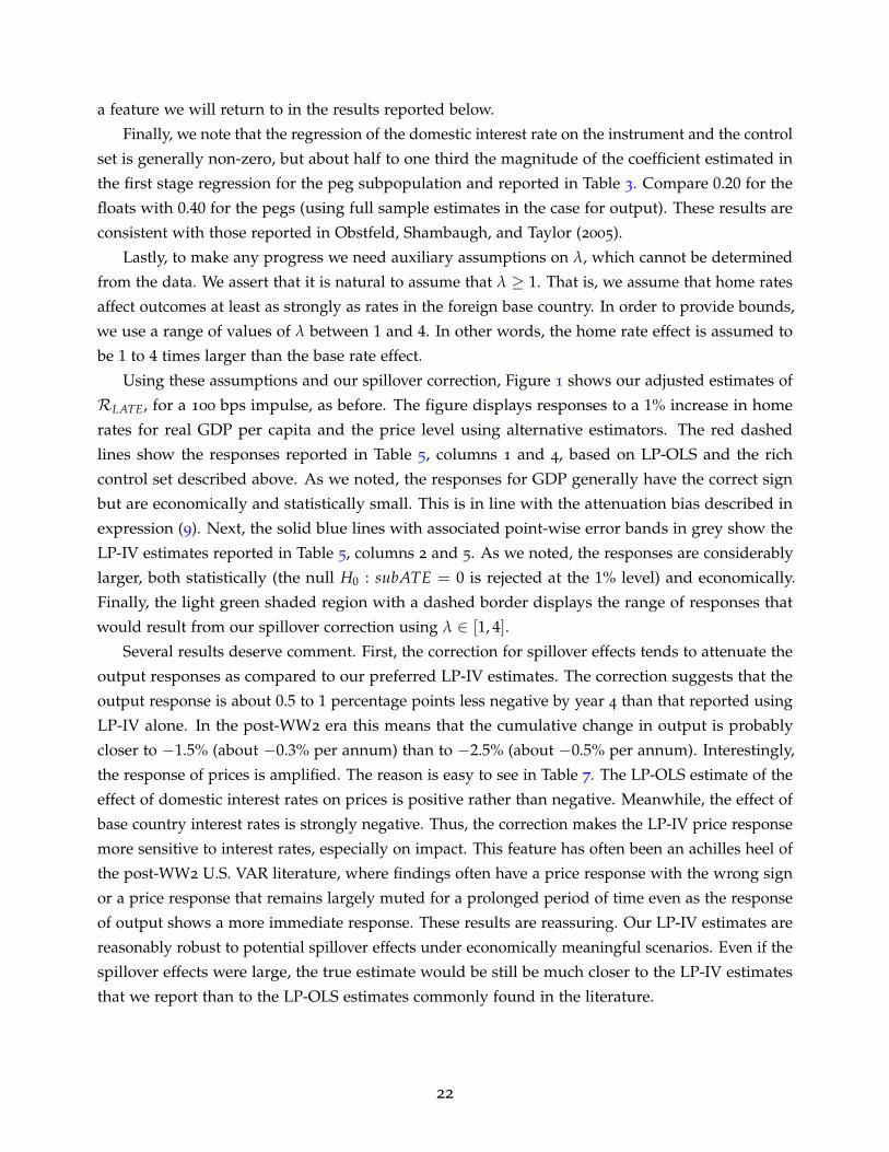
Using these assumptions and our spillover correction, Figure 1 shows our adjusted estimates of
RLATE, for a 100 bps impulse, as before. The figure displays responses to a 1% increase in home
rates for real GDP per capita and the price level using alternative estimators. The red dashed
lines show the responses reported in Table 5, columns 1 and 4, based on LP-OLS and the rich
control set described above. As we noted, the responses for GDP generally have the correct sign
but are economically and statistically small. This is in line with the attenuation bias described in
expression (9). Next, the solid blue lines with associated point-wise error bands in grey show the
LP-IV estimates reported in Table 5, columns 2 and 5. As we noted, the responses are considerably
larger, both statistically (the null H0 : subATE = 0 is rejected at the 1% level) and economically.
Finally, the light green shaded region with a dashed border displays the range of responses that
would result from our spillover correction using λ ∈ [1, 4].
Several results deserve comment. First, the correction for spillover effects tends to attenuate the
output responses as compared to our preferred LP-IV estimates. The correction suggests that the
output response is about 0.5 to 1 percentage points less negative by year 4 than that reported using
LP-IV alone. In the post-WW2 era this means that the cumulative change in output is probably
closer to −1.5% (about −0.3% per annum) than to −2.5% (about −0.5% per annum). Interestingly,
the response of prices is amplified. The reason is easy to see in Table 7. The LP-OLS estimate of the
effect of domestic interest rates on prices is positive rather than negative. Meanwhile, the effect of
base country interest rates is strongly negative. Thus, the correction makes the LP-IV price response
more sensitive to interest rates, especially on impact. This feature has often been an achilles heel of
the post-WW2 U.S. VAR literature, where findings often have a price response with the wrong sign
or a price response that remains largely muted for a prolonged period of time even as the response
of output shows a more immediate response. These results are reassuring. Our LP-IV estimates are
reasonably robust to potential spillover effects under economically meaningful scenarios. Even if the
spillover effects were large, the true estimate would be still be much closer to the LP-IV estimates
that we report than to the LP-OLS estimates commonly found in the literature.
22
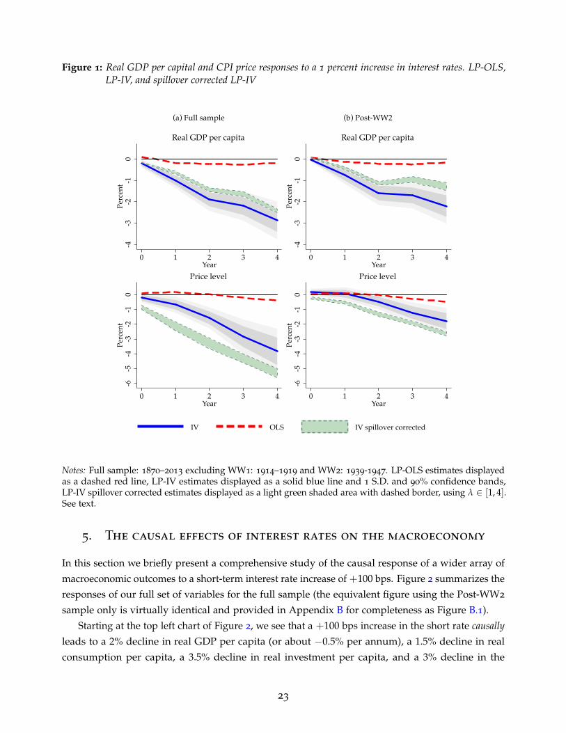
Figure 1: Real GDP per capital and CPI price responses to a 1 percent increase in interest rates. LP-OLS,LP-IV, and spillover corrected LP-IV
-4-3
-2-1
0Pe
rcen
t
0 1 2 3 4Year
Real GDP per capita -6
-5-4
-3-2
-10
Perc
ent
0 1 2 3 4Year
Price level
(a) Full sample
-4-3
-2-1
0Pe
rcen
t
0 1 2 3 4Year
Real GDP per capita
-6-5
-4-3
-2-1
0Pe
rcen
t
0 1 2 3 4Year
Price level
(b) Post-WW2
IV OLS IV spillover corrected
Notes: Full sample: 1870–2013 excluding WW1: 1914–1919 and WW2: 1939-1947. LP-OLS estimates displayedas a dashed red line, LP-IV estimates displayed as a solid blue line and 1 S.D. and 90% confidence bands,LP-IV spillover corrected estimates displayed as a light green shaded area with dashed border, using λ ∈ [1, 4].See text.
5. The causal effects of interest rates on the macroeconomy
In this section we briefly present a comprehensive study of the causal response of a wider array of
macroeconomic outcomes to a short-term interest rate increase of +100 bps. Figure 2 summarizes the
responses of our full set of variables for the full sample (the equivalent figure using the Post-WW2
sample only is virtually identical and provided in Appendix B for completeness as Figure B.1).
Starting at the top left chart of Figure 2, we see that a +100 bps increase in the short rate causallyleads to a 2% decline in real GDP per capita (or about −0.5% per annum), a 1.5% decline in real
consumption per capita, a 3.5% decline in real investment per capita, and a 3% decline in the
23
Figure 2: Full baseline results. Full sample
-3-2
-10
Perc
ent
0 1 2 3 4Year
Real GDP per capita
-3-2
-10
1Pe
rcen
t
0 1 2 3 4Year
Real consumption per capita
-6-4
-20
2Pe
rcen
t
0 1 2 3 4Year
Real investment per capita
-5-4
-3-2
-10
Perc
ent
0 1 2 3 4Year
Price level
-.50
.51
1.5
2Pe
rcen
tage
pts
0 1 2 3 4Year
Short-term interest rate
-.20
.2.4
.6.8
Perc
enta
ge p
ts
0 1 2 3 4Year
Long-term interest rate
-4-2
02
Perc
ent
0 1 2 3 4Year
Real house prices
-10
-50
5Pe
rcen
t
0 1 2 3 4Year
Real stock prices
-2-1
01
2Pe
rcen
t
0 1 2 3 4Year
Private credit/GDP
Notes: Full sample: 1870–2013 excluding WW1: 1914–1919 and WW2: 1939-1947. LP-IV estimates displayedwith a solid blue line and 1 S.D. and 90% confidence bands. See text.
price level (in the second row, first column), where all effects are relative to the no-change policy
counterfactual and the measurements are cumulative over the horizon of 4 years.
Moving along the second row of charts in Figure 2, we look first at the own response of short-
term interest rates to a +100 bps rate rise in year 0 (row 2, column 2). This path reflects the intrinsic
persistence of changes in interest rates. In this case, short-term interest rates increase by +150 bps
in year 1, drop back to +75 bps in year 2, and then decline to effectively zero in both years 3 and 4.
The next chart (row 2, column 3) shows the response of long-term interest rates, which are, as is
well-known, more subdued in amplitude than short rates; the long-term interest rate moves about
half as much. A +100 bps rise in the short rate causally leads to the long rate rising +40 bps in year
1, rising to +60 bps in year 2, and then falling back towards zero by year 4.
Proceeding to the last row of charts in Figure 2 (columns 1 and 2), we can examine the responses
24
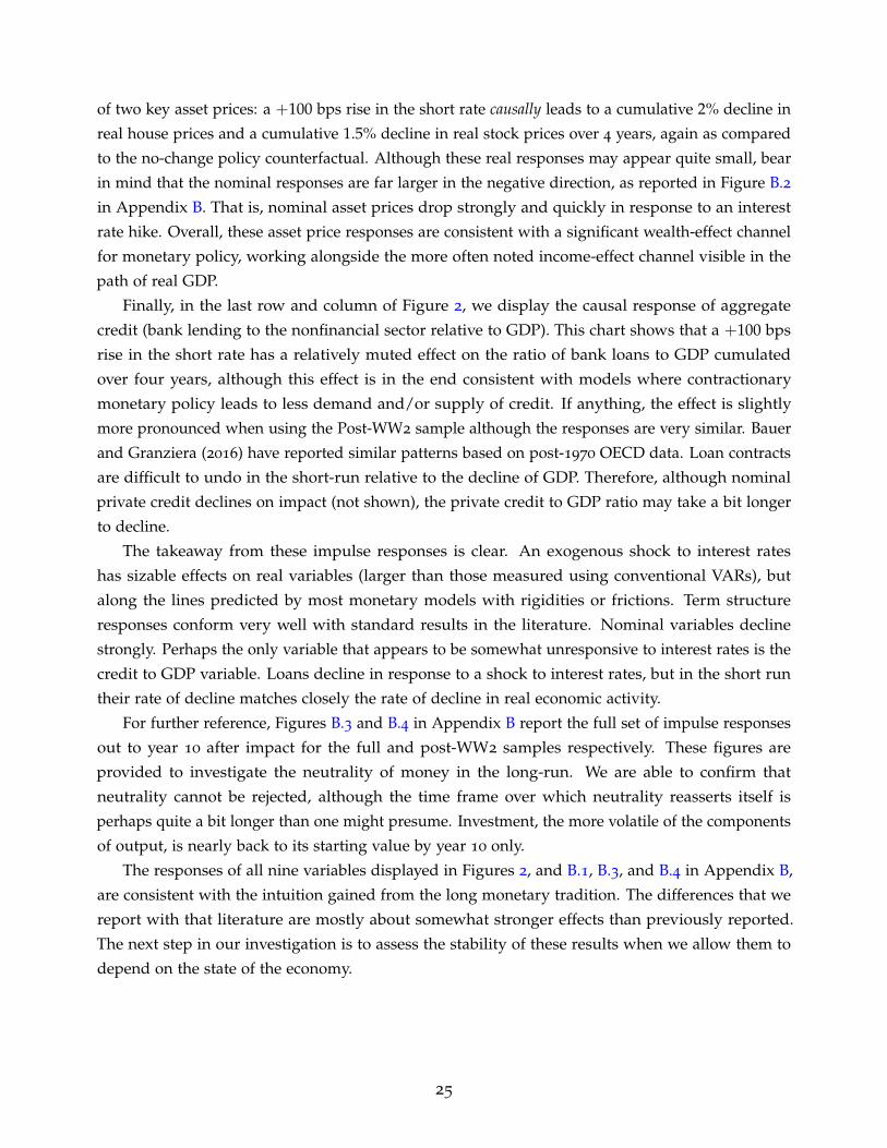
of two key asset prices: a +100 bps rise in the short rate causally leads to a cumulative 2% decline in
real house prices and a cumulative 1.5% decline in real stock prices over 4 years, again as compared
to the no-change policy counterfactual. Although these real responses may appear quite small, bear
in mind that the nominal responses are far larger in the negative direction, as reported in Figure B.2
in Appendix B. That is, nominal asset prices drop strongly and quickly in response to an interest
rate hike. Overall, these asset price responses are consistent with a significant wealth-effect channel
for monetary policy, working alongside the more often noted income-effect channel visible in the
path of real GDP.
Finally, in the last row and column of Figure 2, we display the causal response of aggregate
credit (bank lending to the nonfinancial sector relative to GDP). This chart shows that a +100 bps
rise in the short rate has a relatively muted effect on the ratio of bank loans to GDP cumulated
over four years, although this effect is in the end consistent with models where contractionary
monetary policy leads to less demand and/or supply of credit. If anything, the effect is slightly
more pronounced when using the Post-WW2 sample although the responses are very similar. Bauer
and Granziera (2016) have reported similar patterns based on post-1970 OECD data. Loan contracts
are difficult to undo in the short-run relative to the decline of GDP. Therefore, although nominal
private credit declines on impact (not shown), the private credit to GDP ratio may take a bit longer
to decline.
The takeaway from these impulse responses is clear. An exogenous shock to interest rates
has sizable effects on real variables (larger than those measured using conventional VARs), but
along the lines predicted by most monetary models with rigidities or frictions. Term structure
responses conform very well with standard results in the literature. Nominal variables decline
strongly. Perhaps the only variable that appears to be somewhat unresponsive to interest rates is the
credit to GDP variable. Loans decline in response to a shock to interest rates, but in the short run
their rate of decline matches closely the rate of decline in real economic activity.
For further reference, Figures B.3 and B.4 in Appendix B report the full set of impulse responses
out to year 10 after impact for the full and post-WW2 samples respectively. These figures are
provided to investigate the neutrality of money in the long-run. We are able to confirm that
neutrality cannot be rejected, although the time frame over which neutrality reasserts itself is
perhaps quite a bit longer than one might presume. Investment, the more volatile of the components
of output, is nearly back to its starting value by year 10 only.
The responses of all nine variables displayed in Figures 2, and B.1, B.3, and B.4 in Appendix B,
are consistent with the intuition gained from the long monetary tradition. The differences that we
report with that literature are mostly about somewhat stronger effects than previously reported.
The next step in our investigation is to assess the stability of these results when we allow them to
depend on the state of the economy.
25
6. State dependence
In this section we address the possible state dependence of the impulse-response functions by
stratifying our analysis of output and inflation responses. In particular, we use indicators for
whether the economy is in a boom or slump, in low or high inflation, or in a credit surge or
slowdown, to address big issues from the research literature and current policy debates.
Our first stratification in Figure 3 uses the output gap (“boom/slump”). The boom/slump
stratification delivers a state-dependent analysis that echoes the analysis in Auerbach and Gorod-
nichecko (2013b) and Jorda and Taylor (2016) for fiscal policy, namely, that stabilization policy can
have different effects in the boom (when the output gap is positive) versus the slump (when the
output gap is negative). We measure the gap using a simple low-pass HP filter.
Our second stratification in Figure 4 uses inflation (“high/low”). This links with current debates
about the effectiveness of monetary policy in an environment of unusually low inflation. Despite
widespread belief in the “divine coincidence” (Blanchard and Galı 2005), the returns to ultra-loose
monetary policy are debatable in this setting. Thus, we investigate state dependence based on
high/low inflation environments (defined by an annual 2% CPI inflation rate cutoff).
Our third and final stratification in Figure 5 looks at the growth of credit relative to GDP in the
3 years leading up to the policy intervention, broken down by mortgage versus non-mortgage loans
(adjusted for country-specific variation). The data on credit come from Jorda, Schularick, and Taylor
(2017), and are now publicly available.9 This stratification directly speaks to a nascent literature
that investigates mechanisms by which household/firm heterogeneity in leverage can affect the
effectiveness of monetary policy as discussed in the introduction.
6.1. State dependence in boom and slump episodes
In the first set of nonlinear experiments shown in Figure 3 and Table 8, we set the state variable
equal to 1 in booms and 0 in slumps. Booms (slumps) are years when log real GDP per capita is
above (respectively, below) its long-run country-specific trend component, as measured by an HP
filtered series with a very low-pass setting (λHP=100, annual).
These results are strongly indicative of an asymmetric macroeconomic response to interest rates.
The experiment is always normalized to be a +100 bps increase in the short-term rate. This is done
to facilitate impulse-response comparisons across states even though, of course, tight policy in a
slump is unlikely. The response of real GDP per capita to monetary policy appears to be quite
strong in booms (about −2.5% by year 4, full sample), but considerably weaker in slumps (about
−0.5% by year 4, full sample).
This difference of nearly 2% (closer to 1% Post-WW2) is broadly consistent with Angrist, Jorda,
and Kuersteiner (forthcoming), Tenreyro and Thwaites (2016), and Barnichon and Matthes (2016).
Evidence of asymmetry is less clear for the inflation response, however. Differences using the full
9http://www.macrohistory.net/data/.
26

Figure 3: State dependence: monetary policy has a weaker effect on output in slumps
-4-3
-2-1
0Pe
rcen
t
0 1 2 3 4Year
Real GDP per capita
-6-5
-4-3
-2-1
0Pe
rcen
t
0 1 2 3 4Year
Price level
(a) Full sample
-4-3
-2-1
0Pe
rcen
t
0 1 2 3 4Year
Real GDP per capita
-6-5
-4-3
-2-1
0Pe
rcen
t
0 1 2 3 4Year
Price level
(b) Post-WW2
Baseline
Boom
Slump
Notes: Full sample: 1870–2013 excluding world wars (1914–1919 and 1939–1947). Post-WW2 sample: 1948–2013. Linear LP-IV estimates displayed with a solid blue line and 1 S.D. and 90% confidence bands. Estimatesstratified by the boom displayed with a green dotted line whereas estimates in the slumps are displayed witha red dashed line. See text.
Table 8: Cumulative state-dependent multipliers: ratio of real GDP per capita and CPI inflation responses tothe corresponding interest rate response (percentage points)
Boom Slump Difference
Real GDP per capita -2.7 -0.4 -2.3CPI inflation -3.4 -1.7 -1.7
Notes: Full sample: 1870–2013 excluding world wars (1914–1919 and 1939–1947). The boom (slump) strat-ification refers to years when log real GDP per capita is above (below) its long-run country-specific trendcomponent. The numbers reported can be interpreted as multipliers, that is, how much would cumulativereal GDP per capita (inflation) change in percent (percentage points) on average over the 4 years consideredto construct the impulse responses reported in Figure 3. Percent responses are 100× log. See text.
27
sample are very minor and not very different from the average response. The Post-WW2 responses
suggest that if the monetary authority tried to stimulate the economy (opposite to what is displayed
but consistent with the outlook in many economies today), it would take 2 years before the effects
would be felt in prices, although after 4 years the effects would be similar in size to those estimated
for the boom state.
As a further check, we calculate average multipliers as the average change in percent (for real
GDP per capita) or percentage points (for inflation), relative to the average change in interest rates,
all in response to a one percentage point increase in interest rates. This normalization removes
differences across states that may arise from differences in the interest rate paths in each state. Table
8 summarizes the values of these multipliers and shows that the stark differences shown in Figure 3
are not driven by differences in the policy response paths.
To sum up, a central bank rate tightening of +100 bps in a boom would have causal effects on
output that are strongly contractionary on output going forward. In contrast, a central bank rate
loosening of −100 bps in a slump would have causal effects on output that are, proportionately,
only weakly expansionary. However, the effects on prices would be roughly symmetric across the
two states. Thus, the “sacrifice ratios” for monetary policy are markedly different, and so are the
incentives to pursue pre-emptive monetary policy, in one state versus the other.
6.2. State dependence in “lowflation” episodes
Our next set of nonlinear experiments, in Figure 4 and Table 9, concerns the hypothesis that
monetary policy may have different effects in times of low inflation, a topic of rising interest since
the advanced economies entered an era of “lowflation” as the Great Recession wore on after 2008.
To examine this nonlinearity we chose to set an indicator state variable equal to 1 when inflation is
low (at or below 2%) and 0 otherwise.
These results could be seen as reinforcing some findings in the previous section concerning
differences over the typical output and inflation cycle. Just as in Figure 3, we normalize the responses
to a +100 bps increase in interest rates, while fully recognizing rates are unlikely to go up when
there is lowflation. However, the normalization greatly facilitates the comparison across states. The
response of real GDP to monetary policy appears to be quite strong when inflation is above 2%. In
that scenario, the cumulated response at year 4 is slightly above −3%, somewhat stronger than the
response in booms reported in figure 3, which was −2.5%. However, monetary policy loses most of
its traction when the inflation rate dips below the 2% threshold and economies tip into a lowflation
state. In the full sample results, we find that there is no effect on output although in the Post-WW2
sample, the effect on output is somewhat more visible (around −1%).
For completeness, we compute multipliers similar to those reported in Table 8. That is, we
evaluate the average response of real GDP per capita and inflation relative to that of the interest rate
path, stratified by whether inflation is above of below two percent. These results are reported in
Table 9 and support the results reported in Figure 4.
28
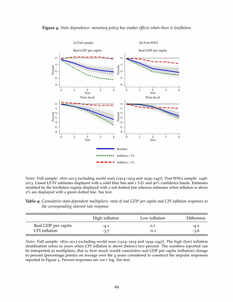
Figure 4: State dependence: monetary policy has weaker effects when there is lowflation
-4-3
-2-1
0Pe
rcen
t
0 1 2 3 4Year
Real GDP per capita
-6-5
-4-3
-2-1
0Pe
rcen
t
0 1 2 3 4Year
Price level
(a) Full sample
-4-3
-2-1
0Pe
rcen
t
0 1 2 3 4Year
Real GDP per capita
-6-5
-4-3
-2-1
0Pe
rcen
t
0 1 2 3 4Year
Price level
(b) Post-WW2
Baseline
Inflation > 2%
Inflation < 2%
Notes: Full sample: 1870–2013 excluding world wars (1914–1919 and 1939–1947). Post-WW2 sample: 1948–2013. Linear LP-IV estimates displayed with a solid blue line and 1 S.D. and 90% confidence bands. Estimatesstratified by the lowflation regime displayed with a red dashed line whereas estimates when inflation is above2% are displayed with a green dotted line. See text.
Table 9: Cumulative state-dependent multipliers: ratio of real GDP per capita and CPI inflation responses tothe corresponding interest rate response
High inflation Low inflation Difference
Real GDP per capita -4.1 0.1 -4.2CPI inflation -3.7 -0.1 -3.6
Notes: Full sample: 1870–2013 excluding world wars (1914–1919 and 1939–1947). The high (low) inflationstratification refers to years when CPI inflation is above (below) two percent. The numbers reported canbe interpreted as multipliers, that is, how much would cumulative real GDP per capita (inflation) changein percent (percentage points) on average over the 4 years considered to construct the impulse responsesreported in Figure 4. Percent responses are 100× log. See text.
29
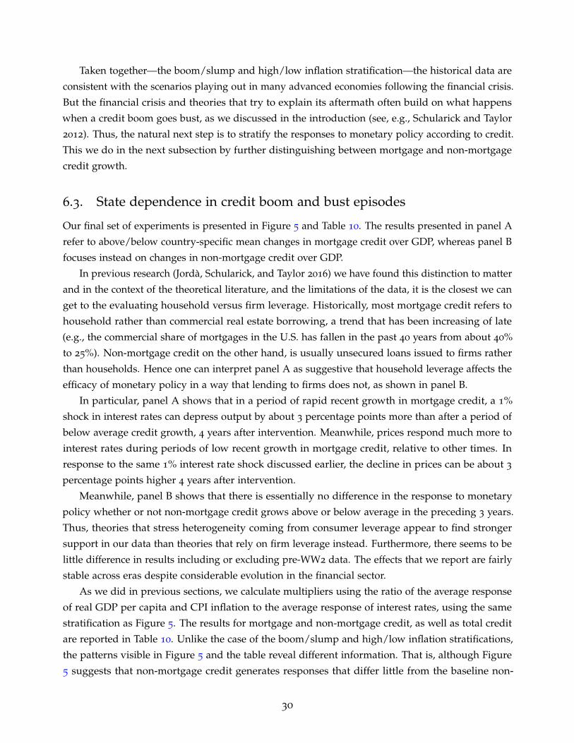
Taken together—the boom/slump and high/low inflation stratification—the historical data are
consistent with the scenarios playing out in many advanced economies following the financial crisis.
But the financial crisis and theories that try to explain its aftermath often build on what happens
when a credit boom goes bust, as we discussed in the introduction (see, e.g., Schularick and Taylor
2012). Thus, the natural next step is to stratify the responses to monetary policy according to credit.
This we do in the next subsection by further distinguishing between mortgage and non-mortgage
credit growth.
6.3. State dependence in credit boom and bust episodes
Our final set of experiments is presented in Figure 5 and Table 10. The results presented in panel A
refer to above/below country-specific mean changes in mortgage credit over GDP, whereas panel B
focuses instead on changes in non-mortgage credit over GDP.
In previous research (Jorda, Schularick, and Taylor 2016) we have found this distinction to matter
and in the context of the theoretical literature, and the limitations of the data, it is the closest we can
get to the evaluating household versus firm leverage. Historically, most mortgage credit refers to
household rather than commercial real estate borrowing, a trend that has been increasing of late
(e.g., the commercial share of mortgages in the U.S. has fallen in the past 40 years from about 40%
to 25%). Non-mortgage credit on the other hand, is usually unsecured loans issued to firms rather
than households. Hence one can interpret panel A as suggestive that household leverage affects the
efficacy of monetary policy in a way that lending to firms does not, as shown in panel B.
In particular, panel A shows that in a period of rapid recent growth in mortgage credit, a 1%
shock in interest rates can depress output by about 3 percentage points more than after a period of
below average credit growth, 4 years after intervention. Meanwhile, prices respond much more to
interest rates during periods of low recent growth in mortgage credit, relative to other times. In
response to the same 1% interest rate shock discussed earlier, the decline in prices can be about 3
percentage points higher 4 years after intervention.
Meanwhile, panel B shows that there is essentially no difference in the response to monetary
policy whether or not non-mortgage credit grows above or below average in the preceding 3 years.
Thus, theories that stress heterogeneity coming from consumer leverage appear to find stronger
support in our data than theories that rely on firm leverage instead. Furthermore, there seems to be
little difference in results including or excluding pre-WW2 data. The effects that we report are fairly
stable across eras despite considerable evolution in the financial sector.
As we did in previous sections, we calculate multipliers using the ratio of the average response
of real GDP per capita and CPI inflation to the average response of interest rates, using the same
stratification as Figure 5. The results for mortgage and non-mortgage credit, as well as total credit
are reported in Table 10. Unlike the case of the boom/slump and high/low inflation stratifications,
the patterns visible in Figure 5 and the table reveal different information. That is, although Figure
5 suggests that non-mortgage credit generates responses that differ little from the baseline non-
30
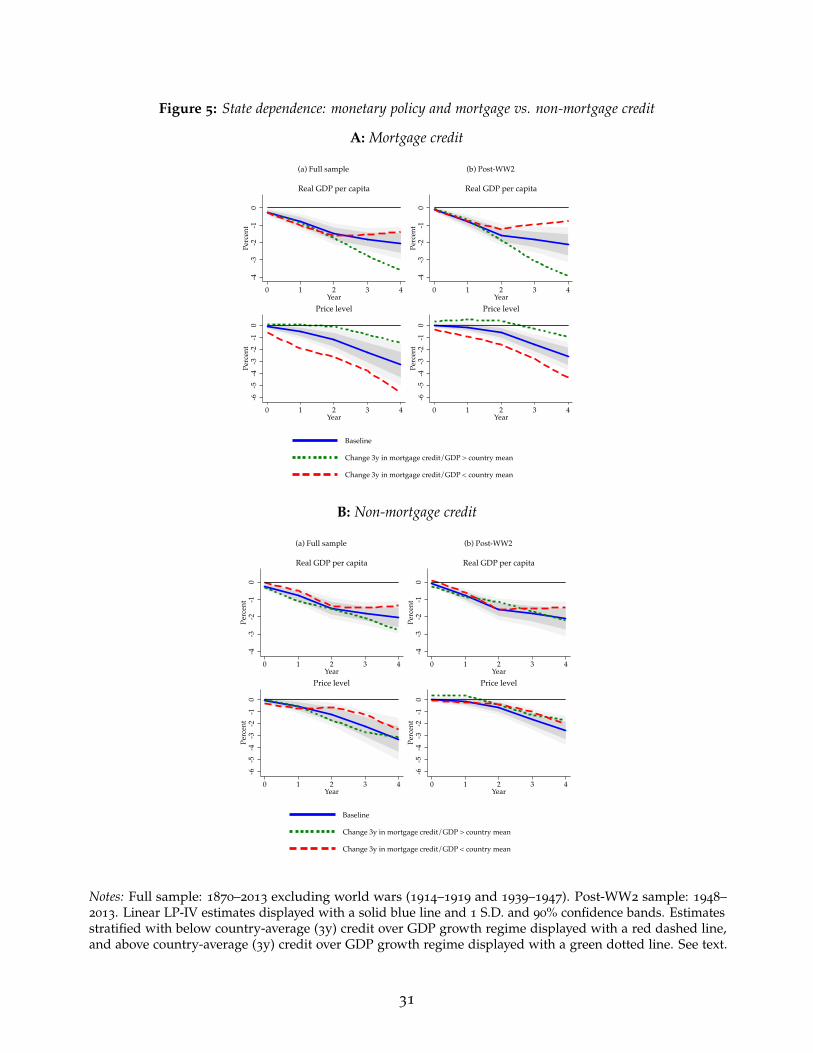
Figure 5: State dependence: monetary policy and mortgage vs. non-mortgage credit
A: Mortgage credit
-4-3
-2-1
0Pe
rcen
t
0 1 2 3 4Year
Real GDP per capita
-6-5
-4-3
-2-1
0Pe
rcen
t
0 1 2 3 4Year
Price level
(a) Full sample
-4-3
-2-1
0Pe
rcen
t
0 1 2 3 4Year
Real GDP per capita
-6-5
-4-3
-2-1
0Pe
rcen
t0 1 2 3 4
Year
Price level
(b) Post-WW2
Baseline
Change 3y in mortgage credit/GDP > country mean
Change 3y in mortgage credit/GDP < country mean
B: Non-mortgage credit
-4-3
-2-1
0Pe
rcen
t
0 1 2 3 4Year
Real GDP per capita
-6-5
-4-3
-2-1
0Pe
rcen
t
0 1 2 3 4Year
Price level
(a) Full sample
-4-3
-2-1
0Pe
rcen
t
0 1 2 3 4Year
Real GDP per capita
-6-5
-4-3
-2-1
0Pe
rcen
t
0 1 2 3 4Year
Price level
(b) Post-WW2
Baseline
Change 3y in mortgage credit/GDP > country mean
Change 3y in mortgage credit/GDP < country mean
Notes: Full sample: 1870–2013 excluding world wars (1914–1919 and 1939–1947). Post-WW2 sample: 1948–2013. Linear LP-IV estimates displayed with a solid blue line and 1 S.D. and 90% confidence bands. Estimatesstratified with below country-average (3y) credit over GDP growth regime displayed with a red dashed line,and above country-average (3y) credit over GDP growth regime displayed with a green dotted line. See text.
31
Table 10: Cumulative state-dependent multipliers: ratio of real GDP per capita and CPI inflation responsesto the corresponding interest rate response
Total credit High credit Low credit Difference
Real GDP per capita -3.7 -0.6 -3.1CPI inflation -1.5 -1.9 0.4
Mortgage credit High credit Low credit Difference
Real GDP per capita -2.7 -2.9 0.2CPI inflation -0.6 -7.2 6.6
Non-mortgage credit High credit Low credit Difference
Real GDP per capita -4.2 -1.1 3.1CPI inflation -4.3 -1.3 -3.0
Notes: Full sample: 1870–2013 excluding world wars (1914–1919 and 1939–1947). The high (low) creditstratification refers to years when credit growth as a ratio to GDP is above (below) country-specific means.The numbers reported can be interpreted as multipliers, that is, how much would cumulative real GDP percapita (inflation) change in percent (percentage points) on average over the 4 years considered to constructthe impulse responses reported in Figure 5. Percent responses are 100× log. See text.
state dependent response, in part this is explained by differences in the path of interest rates.
Moreover, the multipliers reported in Table 10 suggests that there are considerable differences
between mortgage and non-mortgage credit stratifications. The effect of interest rates on output
differs little depending on whether mortgage credit growth is fast or slow, but the differences are
stark with non-mortgage credit. And the effect on inflation goes in the opposite direction.
7. Conclusion
The effectiveness of monetary stabilization policy is not only a major policy concern but also an
important matter of ongoing controversy among both theoretical and empirical macroeconomists.
This paper argues that interest rates can have a considerable effect on macroeconomic outcomes.
The source of the attenuation bias that we report suggests that common assumptions, often based on
regression control arguments (conditional mean independence), do not provide an adequate basis
for identification. Using a quasi-natural experiment in international finance and novel empirical
methods, we show why this bias occurs and how to resolve it.
Monetary stabilization policy turns out to be state-dependent, a critical observation in the
context of the Great Recession and its aftermath. Policymakers have faced a situation of consistent
undershoot relative to their stated objectives and forecasts. A slower than expected growth trajectory
has been seen in the U.S. economy, and worse yet in the U.K., Europe, and Japan; and we have
seen persistent sub-2% inflation afflicting all of these economies. Amid worries of deflation risk and
secular stagnation, the extensive and unconventional application of monetary policy tools has failed
32
to shunt the macroeconomic locomotive onto a faster track. Debate centers on why the central banks
got so derailed, and the subsequent lack of policy traction.
Empirical evidence from the largest advanced economy macroeconomic dataset ever assembled
shows that all of these travails are, in a sense, nothing new. In conditions where output is weak,
inflation is low, or credit is stagnant, the task of stimulating the economy out of its torpor is much
more difficult. These challenging conditions have been seen in many western economies for almost
a decade, but they were also present in the distant past with similar consequences. Our results
therefore have profound implications for how today’s monetary models are formulated and applied.
References
Angrist, Joshua D., Guido W. Imbens, and Donald B. Rubin. 1996. Identification of Causal EffectsUsing Instrumental Variables. Journal of the American statistical Association 91(434): 444–55.
Angrist, Joshua D., Oscar Jorda, and Guido Kuersteiner. Semiparametric Estimates of MonetaryPolicy Effects: String Theory Revisited. Journal of Business and Economic Statistics. Forthcoming.
Auclert, Adrien. 2017. Monetary Policy and the Redistribution Channel. NBER Working Paper23451.
Auerbach, Alan J., and Yuriy Gorodnichenko. 2013a. Measuring the Output Responses to FiscalPolicy. American Economic Journal: Economic Policy 4(2): 1–27.
Auerbach, Alan J., and Yuriy Gorodnichenko. 2013b. Fiscal Multipliers in Recession and Expansion.In Fiscal Policy After the Financial Crisis edited by Alberto Alesina and Francesco Giavazzi.Chicago: University of Chicago Press, pp. 63–98.
Barnichon, Regis, and Christian Matthes. 2016. Gaussian Mixture Approximations of ImpulseResponses and The Non-Linear Effects of Monetary Shocks. CEPR Discussion Paper 11374.
Barro, Robert J., and Jose F. Ursua. 2008. Macroeconomic Crises since 1870. Brookings Papers onEconomic Activity 39(1): 255–335.
Bauer, Gregory H., and Eleonora Granziera. 2016. Monetary Policy, Private Debt, and FinancialStability Risks. International Journal of Central Banking conference in San Francisco. November21–22, 2016.
Bernanke, Ben S. and Mark Gertler. 1995. Inside the Black Box: The Credit Channel of MonetaryTransmission. Journal of Economic Perspectives 9(4): 27–48.
Blanchard, Olivier, and Jordi Galı. Real Wage Rigidities and the New Keynesian Model. 2007. Journalof Money, Credit and Banking 39(S1): 35–65.
Christiano, Lawrence J., Martin S. Eichenbaum, and Charles L. Evans. 1999. Monetary Policy Shocks:What Have We Learned And To What End? Handbook of Macroeconomics, vol. 1, edited by John B.Taylor and Michael Woodford. Amsterdam: Elsevier, pp. 65–148.
Cloyne, James, Clodomiro Ferreira, and Paolo Surico. 2015. Monetary Policy when Householdshave Debt: New Evidence on the Transmission Mechanism. CEPR Discussion Paper 11023.
Cloyne, James, and Patrick Hurtgen. 2016. The Macroeconomic Effects of Monetary Policy: A NewMeasure for the United Kingdom. American Economic Journal: Macroeconomics 8(4): 75–102.
Coibion, Olivier, Yuriy Gorodnichenko, Lorenz Kueng, and John Silvia. 2017. Innocent Bystanders?Monetary Policy and Inequality in the U.S. Journal of Monetary Economics 88: 70–88.
Conley, Timothy G., Christian B. Hansen, and Peter E. Rossi. 2012. Plausibly Exogenous. Review ofEconomics and Statistics 94(1): 260–72.
33
Cox, David R. 1958. Planning of Experiments. New York: John Wiley.di Giovanni, Julian, Justin McCrary, and Till von Wachter. 2009. Following Germany’s Lead: Using
International Monetary Linkages to Estimate the Effect of Monetary Policy on the Economy.Review of Economics and Statistics 91(2): 315–31.
di Giovanni, Julian, and Shambaugh, Jay C. 2008. The Impact of Foreign Interest Rates on theEconomy: The Role of the Exchange Rate Regime. Journal of International Economics 74(2): 341–61.
Eichenbaum, Martin S. 1992. Comments ‘Interpreting the Macroeconomic Time Series Facts: TheEffects of Monetary Policy’ by Christopher Sims. European Economic Review 36(5): 1001–11.
Faust, Jon, Eric T. Swanson, and Jonathan H. Wright. 2004. Identifying VARs Based on HighFrequency Futures Data. Journal of Monetary Economics 51(6): 1107–31.
Gertler, Mark, and Peter Karadi. 2015. Monetary Policy Surprises, Credit Costs, and EconomicActivity. American Economic Journal: Macroeconomics 7(1): 44–76.
Gurkaynak, Refet S., Brian Sack, and Eric Swanson. 2005. The Sensitivity of Long-Term InterestRates to Economic News: Evidence and Implications for Macroeconomic Models. AmericanEconomic Review 95(1): 425–36.
Hanson, Michael S. 2004. The ”Price Puzzle” Reconsidered. Journal of Monetary Economics 51(7):1385–1413.
Hanson, Samuel G., David O. Lucca and Jonathan H. Wright. 2017. Interest Rate Conundrums inthe Twenty-First Century. FRBNY Staff Report no. 810.
Iacoviello, Matteo. 2005. House Prices, Borrowing Constraints, and Monetary Policy in the BusinessCycle. American Economic Review 95(3): 739–764.
Imbens, Guido W. 2014. Instrumental Variables: An Econometrician’s Perspective. NBER WorkingPaper 19983.
Imbens, Guido W., and Joshua Angrist. 1994. Identification and Estimation of Local AverageTreatment Effects. Econometrica 61(2): 467–76.
Ilzetzki, Ethan, Enrique G. Mendoza, and Carlos A. Vegh. 2013. How Big (Small?) are FiscalMultipliers? Journal of Monetary Economics 60(2): 239–54.
Jorda, Oscar. 2005. Estimation and Inference of Impulse Responses by Local Projections. AmericanEconomic Review 95(1): 161–82.
Jorda, Oscar, Moritz Schularick, and Alan M. Taylor. 2015. Betting the House. Journal of InternationalEconomics 96(S1): S2–S18.
Jorda, Oscar, Moritz Schularick, and Alan M. Taylor. 2016. The Great Mortgaging: Housing Finance,Crises and Business Cycles. Economic Policy 31(85): 107–152.
Jorda, Oscar, Moritz Schularick, and Alan M. Taylor. 2017. Macrofinancial History and the NewBusiness Cycle Facts. NBER Macroeconomics Annual 2016, no. 31, edited by Martin Eichenbaumand Jonathan A. Parker. Chicago: University of Chicago Press. Forthcoming.
Jorda, Oscar, and Alan M. Taylor. 2016. The Time for Austerity: Estimating the Average TreatmentEffect of Fiscal Policy. Economic Journal 126(590): 219–55.
Kaplan, Greg, Benjamin Moll and Giovanni L. Violante. 2016. Monetary Policy According to HANK.NBER Working Paper 21897
Kashyap, Anil K., Owen A. Lamont, and Jeremy C. Stein. 1994. Credit Conditions and the CyclicalBehavior of Inventories. Quarterly Journal of Economics 109(3): 565–593.
Kashyap, Anil K., and Jeremy C. Stein. 1995. The Impact of Monetary Policy on Bank Balance Sheets.Carnegie-Rochester Conference Series on Public Policy 42: 151–19.
Knoll, Katharina, Moritz Schularick, and Thomas Steger. No Price Like Home: Global House Prices,1870–2012. American Economic Review 107(2): 331–53.
Kuttner, Kenneth N. 2001. Monetary Policy Surprises and Interest Rates: Evidence from the FedFunds Futures Market. Journal of Monetary Economics 47(3): 523–44.
34
Nakamura, Emi, and Jon Steinsson. 2013. High Frequency Identification of Monetary Non-Neutrality.Quarterly Journal of Economics. Forthcoming.
Obstfeld, Maurice, and Kenneth Rogoff. 1995. The Mirage of Fixed Exchange Rates. Journal ofEconomic Perspectives 9(4): 73–96.
Obstfeld, Maurice, Jay C. Shambaugh, and Alan M. Taylor. 2004. Monetary Sovereignty, ExchangeRates, and Capital Controls: The Trilemma in the Interwar Period. IMF Staff Papers 51(S): 75–108.
Obstfeld, Maurice, Jay C. Shambaugh, and Alan M. Taylor. 2005. The Trilemma in History: Tradeoffsamong Exchange Rates, Monetary Policies, and Capital Mobility. Review of Economics and Statistics87(3): 423–38.
Obstfeld, Maurice, and Alan M. Taylor. 1998. The Great Depression as a Watershed: InternationalCapital Mobility in the Long Run. In The Defining Moment: The Great Depression and the AmericanEconomy in the Twentieth Century, edited by Michael D. Bordo, Claudia D. Goldin, and Eugene N.White. Chicago: University of Chicago Press.
Obstfeld, Maurice, and Alan M. Taylor. 2004. Global Capital Markets: Integration, Crisis, and Growth.Japan-U.S. Center Sanwa Monographs on International Financial Markets. Cambridge: Cam-bridge University Press.
Ottonello, Pablo, and Thomas Winberry. 2017. Financial Heterogeneity and the Investment Channelof Monetary Policy. University of Michigan. Unpublished.
Owyang, Michael T., Valerie A. Ramey, and Sarah Zubairy. 2013. Are Government SpendingMultipliers Greater during Periods of Slack? Evidence from Twentieth-Century Historical Data.American Economic Review 103(3): 129–34.
Quinn, Dennis P., Martin Schindler, and A. Maria Toyoda. 2011. Assessing Measures of FinancialOpenness and Integration. IMF Economic Review 59(3): 488–522.
Ramey, Valerie A. 2016. Macroeconomic Shocks and Their Propagation. In Handbook of Macroeco-nomics, Volume 2, edited by J. B. Taylor and H. Uhlig. Amsterdam: Elsevier, pp. 71–162.
Ramey, Valerie A., and Sarah Zubairy. 2014. Government Spending Multipliers in Good Times andin Bad: Evidence from US Historical Data. NBER Working Paper 20719.
Romer, Christina D. and David H. Romer. 1989 Does Monetary Policy Matter? A New Test in theSpirit of Friedman and Schwartz. NBER Macroeconomics Annual 4: 121–70.
Romer, Christina D. and David H. Romer. 2004. A New Measure of Monetary Shocks: Derivationand Implications. American Economic Review 94(4): 1055–84.
Rubin, Donald B. 1974. Estimating Causal Effects of Treatments in Randomized and NonradomizedStudies. Journal of Educational Psychology 66(5): 688–701.
Rubin, Donald B. 1978. Bayesian Inference for Causal Effects: The Role of Randomization. Annals ofStatistics 6(1): 34–58.
Rubin, Donald B. 2005. Causal Inference Using Potential Outcomes: Design, Modeling, Decisions.Journal of the American Statistical Association 100(469): 322–331.
Shambaugh, Jay C. 2004. The Effect of Fixed Exchange Rates on Monetary Policy. Quarterly Journalof Economics 119(1): 301–352.
Sims, Christopher A. 1992. Interpreting the Macroeconomic Time Series Facts: The Effects ofMonetary Policy. European Economic Review 36(5): 975–1000.
Swanson, Eric T., and John C. Williams. 2014. Measuring the Effect of the Zero Lower Bound onMedium- and Longer-Term Interest Rates. American Economic Review 104(10): 3154–85.
Tenreyro, Silvana, and Gregory Thwaites. 2016. Pushing on a String: US Monetary Policy is LessPowerful in Recessions. American Economic Journal: Macroeconomics. 8(4): 43–74.
Wooldridge, Jeffrey M. 2015. Control Function Methods in Applied Econometrics. Journal of HumanResources 50(2): 420–45.
35
Appendices
A. Evaluating the exclusion restriction: general caseDetailed derivations of the results in Section 3.2 are provided for a panel of data. Denote the genericdimensions of the panel for each subpopulation considered as N for the cross section and T for thetime series dimension. Different subpopulations will have different dimensions but, in the interestof clarity, we refrain from using subscripts for now.
In our application, we use the auxiliary subpopulation of floats to correct the IV estimates basedon the peg subpopulation for spillover bias. The consistency results are based on N, T → ∞ for bothof these subpopulations. Because we do not need inferential procedures (ours is a robustness checkto examine the potential biases from spillover effects) we do not derive the asymptotic distributionof the bias corrected estimator. In other settings, auxiliary information may be available that wouldallow one to obtain point-identified bias corrections. The derivations provided here could be readilyextended to derive the asymptotic distribution.
To simplify the notation, consider the non-state dependent version of expression (5), extended toinclude potential spillovers:
∆ri,t = ai + zi,tb + xi,tg + ηi,t ,
yi,t+h = αhi + ∆ri,tβh + zi,tφ + xi,tγh + νi,t+h ; h = 0, 1, ..., H . (11)
We make standard regularity assumptions about the error processes and assume, in particular, thatthe following moment conditions hold E(zi,tηi,t) = E(zi,tνi,t+h) = 0. That is, zi,t is an exogenouslydetermined valid instrument.
Next, define the projection matrix Mi,t = 1−wi,t(w′i,twi,t)−1w′i,t, where w includes the fixed
effects and the x, but excludes z and ∆r. Pre-multiplying expression (11) by Mi,t allows us to focuson the coefficients of interest, b, βh, and φ. For example, using this projection matrix, note that theOLS estimator of b is simply
b =
(1
NT
T
∑t=1
N
∑i=1
zi,t Mi,tzi,t
)−1(1
NT
T
∑t=1
N
∑i=1
zi,t Mi,t∆ri,t
).
An additional piece of notation will help make the derivations that follow more transparent.Consider the moment condition E(zi,t Mi,tηi,t) = 0. We define the operator
S(z, η) =
(1
NT
T
∑t=1
N
∑i=1
zi,t Mi,tηi,t
)p→ E(zi,t Mi,tηi,t)
as a way to refer to the equivalent sample moment condition implied by the population statement.Using this operator and the usual OLS moment conditions, it is easy to see that
βh =S(z, ∆r) S(z, y(h))− S(z2) S(∆r, y(h))
S(z, ∆r)2 − S(z2) S(∆r2), (12)
φ =S(z, ∆r) S(∆r, y(h))− S(∆r2) S(z, y(h))
S(z, ∆r)2 − S(z2) S(∆r2). (13)
36
These moment conditions rely on the usual OLS assumptions E(∆ri,t Mi,tνi,t+h) = 0, andE(zi,t Mi,tνi,t+h) = 0. However, here we explore what happens to estimators that assume theseconditions but where in reality the first moment condition is violated due to the endogeneity of∆ri,t. In that case, OLS estimates of βh and φ based on (12) and (13) will be biased.
In particular, we can define the bias term
θ =S(z2) S(∆r, ν(h))
S(z, ∆r)2 − S(z2) S(∆r2)
p→ θ .
It is then straightforward to show using expressions (12) and (13) that
βhp→ βh − θ ,
φp→ φ + bθ ,
where we made use of the standard OLS result
b =S(z, ∆r)
S(z2)
p→ b . (14)
Notice that under the assumptions of the model, this estimator is consistent for b. Next, withoutloss of generality, let βh = λφ, for λ an unrestricted parameter. Then, it is easy to show that
φ(λ) =bβh + φ
1 + λbp→ φ(λ) . (15)
In practice the true value of λ is unknown. The approach that we follow here is to calculateexpression (15) for a range of values of λ ∈ [λ, λ]. Because λ is unknown, we do not attempt tocharacterize the asymptotic distribution of our spillover corrected estimator.
The next step consists of incorporating φ(λ), which is based on the float subpopulation, tocorrect the IV estimator for the subpopulation of pegs. The control function approach consists inusing the usual IV estimator on the following auxiliary expression:
y∗i,t+h = ∆ri,tβh + xi,tγh + ui,t+h ,
y∗i,t+h ≡ (yi,t+h − zi,tφ(λ)) ,
ui,t+h ≡ νi,t+h + zi,t(φ(λ))− φ(λ))) .
Consistency of this modified IV estimator only requires the usual consistency conditions of IVestimators applied to the sample of pegs. Notice that if φ(λ)→ φ(λ), then(
1NT
T
∑t=1
N
∑i=1
zi,t Mi,tzi,t
)(φ(λ))− φ(λ))
p→ 0 if E(z M z) < ∞ .
This is the condition that, along with the typical IV conditions, ensures consistency for βh asN, T → ∞ in both the peg and the float subpopulations.
37

B. Robustness checksFigures B.1 through B.4 in this appendix contain a series of robustness check which are mentionedin the main text.
38
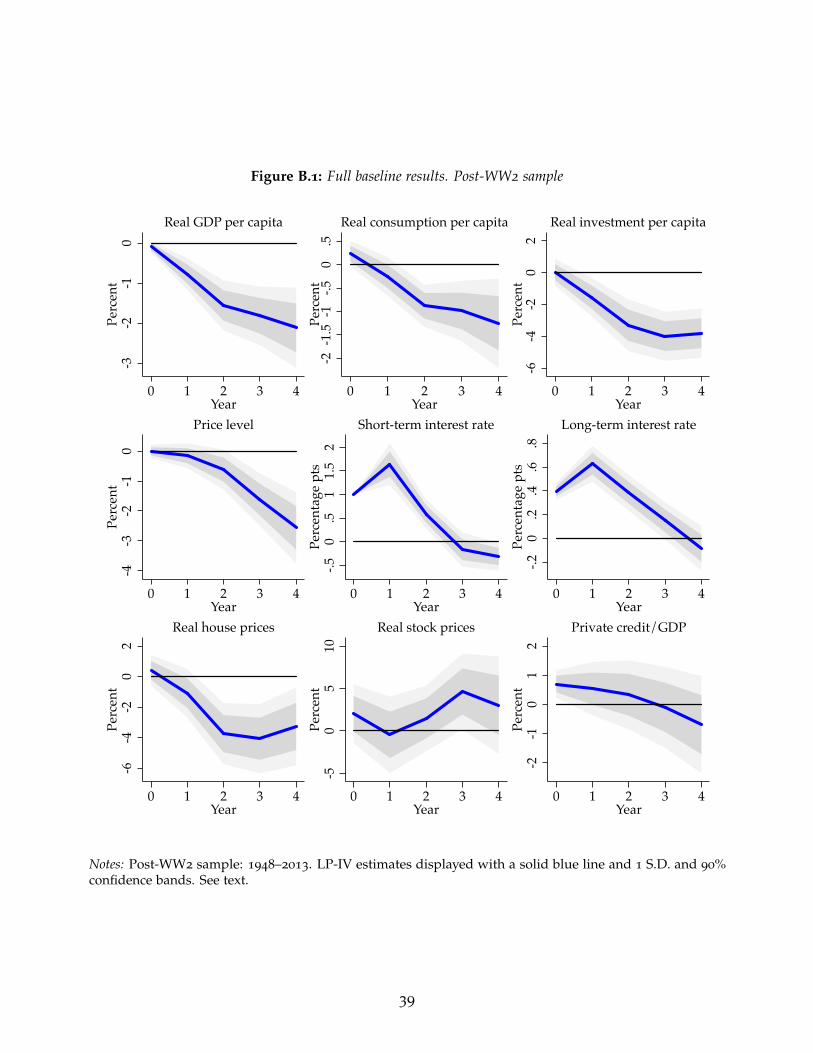
Figure B.1: Full baseline results. Post-WW2 sample
-3-2
-10
Perc
ent
0 1 2 3 4Year
Real GDP per capita
-2-1
.5-1
-.50
.5Pe
rcen
t
0 1 2 3 4Year
Real consumption per capita
-6-4
-20
2Pe
rcen
t
0 1 2 3 4Year
Real investment per capita
-4-3
-2-1
0Pe
rcen
t
0 1 2 3 4Year
Price level
-.50
.51
1.5
2Pe
rcen
tage
pts
0 1 2 3 4Year
Short-term interest rate
-.20
.2.4
.6.8
Perc
enta
ge p
ts
0 1 2 3 4Year
Long-term interest rate
-6-4
-20
2Pe
rcen
t
0 1 2 3 4Year
Real house prices
-50
510
Perc
ent
0 1 2 3 4Year
Real stock prices
-2-1
01
2Pe
rcen
t
0 1 2 3 4Year
Private credit/GDP
Notes: Post-WW2 sample: 1948–2013. LP-IV estimates displayed with a solid blue line and 1 S.D. and 90%confidence bands. See text.
39
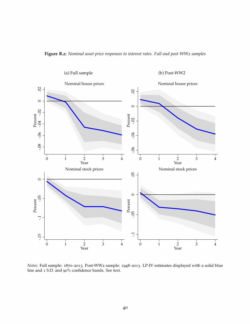
Figure B.2: Nominal asset price responses to interest rates. Full and post-WW2 samples
-.08
-.06
-.04
-.02
0.0
2Pe
rcen
t
0 1 2 3 4Year
Nominal house prices
-.15
-.1-.0
50
Perc
ent
0 1 2 3 4Year
Nominal stock prices
(a) Full sample
-.06
-.04
-.02
0.0
2Pe
rcen
t
0 1 2 3 4Year
Nominal house prices
-.1-.0
50
.05
Perc
ent
0 1 2 3 4Year
Nominal stock prices
(b) Post-WW2
Notes: Full sample: 1870–2013. Post-WW2 sample: 1948–2013. LP-IV estimates displayed with a solid blueline and 1 S.D. and 90% confidence bands. See text.
40
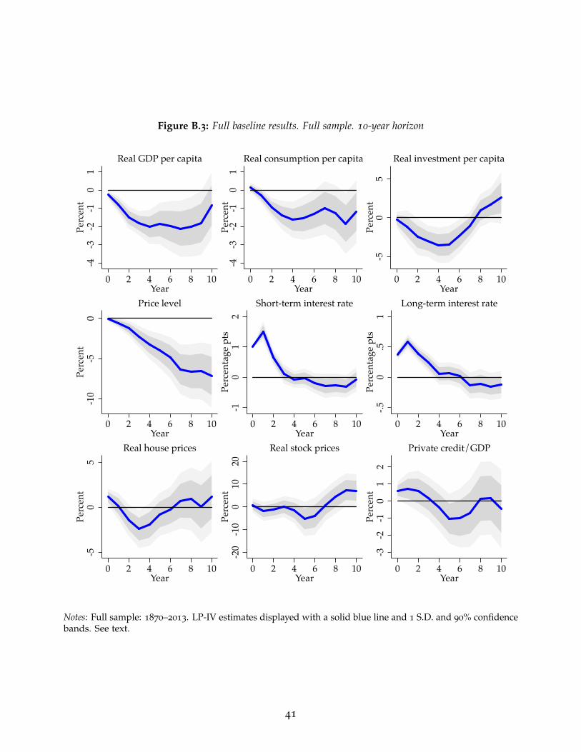
Figure B.3: Full baseline results. Full sample. 10-year horizon
-4-3
-2-1
01
Perc
ent
0 2 4 6 8 10Year
Real GDP per capita
-4-3
-2-1
01
Perc
ent
0 2 4 6 8 10Year
Real consumption per capita
-50
5Pe
rcen
t
0 2 4 6 8 10Year
Real investment per capita
-10
-50
Perc
ent
0 2 4 6 8 10Year
Price level
-10
12
Perc
enta
ge p
ts
0 2 4 6 8 10Year
Short-term interest rate
-.50
.51
Perc
enta
ge p
ts
0 2 4 6 8 10Year
Long-term interest rate
-50
5Pe
rcen
t
0 2 4 6 8 10Year
Real house prices
-20
-10
010
20Pe
rcen
t
0 2 4 6 8 10Year
Real stock prices
-3-2
-10
12
Perc
ent
0 2 4 6 8 10Year
Private credit/GDP
Notes: Full sample: 1870–2013. LP-IV estimates displayed with a solid blue line and 1 S.D. and 90% confidencebands. See text.
41
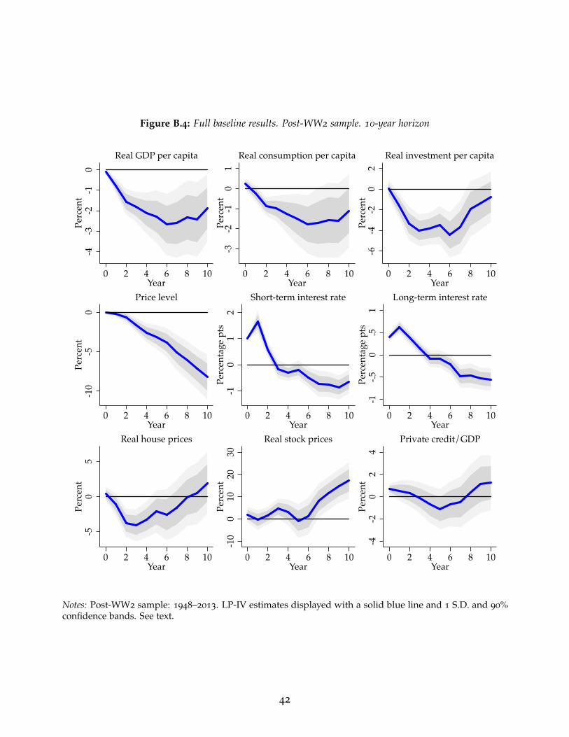
Figure B.4: Full baseline results. Post-WW2 sample. 10-year horizon
-4-3
-2-1
0Pe
rcen
t
0 2 4 6 8 10Year
Real GDP per capita
-3-2
-10
1Pe
rcen
t
0 2 4 6 8 10Year
Real consumption per capita
-6-4
-20
2Pe
rcen
t
0 2 4 6 8 10Year
Real investment per capita
-10
-50
Perc
ent
0 2 4 6 8 10Year
Price level
-10
12
Perc
enta
ge p
ts
0 2 4 6 8 10Year
Short-term interest rate
-1-.5
0.5
1Pe
rcen
tage
pts
0 2 4 6 8 10Year
Long-term interest rate
-50
5Pe
rcen
t
0 2 4 6 8 10Year
Real house prices
-10
010
2030
Perc
ent
0 2 4 6 8 10Year
Real stock prices
-4-2
02
4Pe
rcen
t
0 2 4 6 8 10Year
Private credit/GDP
Notes: Post-WW2 sample: 1948–2013. LP-IV estimates displayed with a solid blue line and 1 S.D. and 90%confidence bands. See text.
42
Recommended


![QUASI-BIGEBRES DE LIE ET ALGEBRES QUASI-BATALIN ...streaming.ictp.it/preprints/P/99/174.pdf3 Quasi-bigebres de Lie Les quasi-bigebres de Lie [6] (appelees quasi-bigebres jacobiennes](https://img.pdfslide.us/doc/110x75/60aa5fd4a787df4f051abfc1/quasi-bigebres-de-lie-et-algebres-quasi-batalin-3-quasi-bigebres-de-lie-les.jpg)