1
The Effects of Quantitative Easing on Long-term Interest Rates Arvind Krishnamurthy 1 and Annette Vissing-Jorgensen 2
November 8, 2010
Abstract: We evaluate the effect of the Federal Reserve’s purchase of long-term Treasuries and
other long-term bonds ("QE1" in 2008-2009 and "QE2" in 2010) on nominal and real long-term
interest rates. We find a large and significant drop in nominal interest rates on long-term safe
assets (Treasuries and Agencies bonds). This occurs partly because there is a unique clientele
for long-term safe nominal assets, and the Fed purchases reduce the supply of long-term safe
assets and hence increase the safety-premium that such investors will pay for such assets. We
find a much smaller effect on the nominal interest rates on less safe assets such as Baa corporate
rates and mortgage rates (likely driven by lowered duration risk premia). These are rates more
relevant for long-term borrowing by corporations and households. Our analysis indicates that it is
inappropriate to focus only on Treasury rates as a policy target because the effects of purchases
on the duration risk premium are small, while effects on safety/liquidity premia are more
substantial. Furthermore, evidence from inflation swap rates show that expected inflation
increased substantially as a result of QE1, but did not change measurably as a result of QE2,
implying that reductions in real rates were much larger than reductions in nominal rates for QE1
but not QE2. We estimate that QE1 reduced real, default-adjusted Baa corporate rates by 112
bps, while the effect of QE2 on this rate was a reduction of only 9 bps.
1 Kellogg School of Management, Northwestern University and NBER 2 Kellogg School of Management, Northwestern University, NBER and CEPR

2
1. Introduction
The Federal Reserve has recently pursued the unconventional policy of purchasing large
quantities of long-term Treasuries (quantitative easing, or “QE”). The objective of this paper is to
evaluate the impact of QE on various long-term rates given two pieces of information: (a)
Knowledge about the relevant features of long and short-term Treasuries from the analysis by
Krishnamurthy and Vissing-Jorgensen (2010) (hereafter, KVJ). (b) Analysis of the effects of
long-term asset purchases by the Federal Reserve in the late-2008 to 2009 period (“QE1”), and
announcements regarding purchases in late-2010 (“QE2”) interpreted in the light of this
knowledge.
The stated objective of quantitative easing is to reduce long-term interest rates in order to spur
economic activity.3
The QE2 strategy involves purchasing long-term Treasuries and paying by
increasing reserve balances. Interest bearing reserve balances can be thought of as overnight
government debt. Thus, a $600bn QE2 decreases long-term Treasury supply by $600bn and
increases overnight debt supply by $600bn. The common argument for how this policy may
affect interest rates is based on portfolio balance: The Fed reduces the portfolio of long-term
versus short-term bonds in the hands of investors and thereby lowers long-rates relative to short-
rates.
Our analysis in KVJ offers two important points for appraising these issues: (1) We show that it
is important to ask which interest rate (i.e. Treasury, Agency, MBS, Baa, etc.) will be affected by
the policy move; and (2) We show that the asset purchased (i.e. Treasuries, Agency, MBS, etc.)
in the policy matters for outcomes.
In our framework, changes in the overall supply of Treasuries affect interest rates through a
liquidity channel and through a safety channel. Investors have a unique demand for liquid and
safe assets and thus place a premium on these assets, above and beyond what they would be
willing to pay according to standard CCAPM models.4
3 http://www.newyorkfed.org/newsevents/speeches/2010/dud101001.html
Altering the supply of Treasuries
4 A simply way to think about investor willingness to pay extra for assets with very low default risk is to plot the price against the expected default rate. KVJ argue that this curve is very steep for low default rates, with a slope that flattens as the supply of Treasuries increases.

3
changes the supply of liquid and safe assets in the hands of investors, changing the liquidity and
safety premium, and thereby changing interest rates. These effects are only present in safe
and/or liquid bonds (e.g. Treasuries, Agencies, and highly rated corporate bonds). This is
important for thinking about QE because, while there is considerable evidence for supply effects,
most of the evidence comes from examining the behavior of Treasury interest rates, or other near
safe/liquid substitutes.5 But, even if a policy affects Treasury interest rates, such rates may not
be policy relevant. Most economic activity is funded by debt that is not as free of credit risk as
Treasuries, Agencies, Aaas. For example, only a small fraction of corporate bonds are rated Aaa
or Aa, with the majority of corporate debt being A, Baa, or lower. If the objective of QE is to
reduce interest rates paid by the majority of corporations and households which may then spur
spending and economic growth, then examining supply effects on Treasury rates will be
misleading.6
Indeed, looking at the effect of supply on Baa rates is the most relevant benchmark.
(KVJ focus on Baa rated bonds as the benchmark, as opposed to A or C rated bonds, because the
yield on Baa corporate bonds is available back to 1919. Longstaff, Mithal and Neis (2006) use
credit default swap data from December 2000 to October 2001 to show that the non-default
component of yields is about 50 bps for Aaa and Aa rated bonds, and about 70 bps for lower-
rated bonds, suggesting that the cutoff for bonds whose yields are not affected by liquidity or
safety premia is somewhere around the A rating.).
In theory, supply can affect even Baa rates through a duration-risk channel. By purchasing long-
term Treasuries, policy can reduce the duration risk in the hands of investors and thereby affect
the term premium (i.e. the risk premium between long-term bonds and short-term bonds). The
KVJ analysis does not account for any effects on the duration risk premium. This is because the
evidence in KVJ is based on examining the effects of Treasury supply on maturity-matched
spreads between non-Treasury (i.e. corporate) bonds and Treasury bonds. Greenwood and
Vayanos (2010) offer evidence for how a change in the supply of Treasuries affects the spread
between long-term and short-term Treasury bonds. Their demonstrated effect has been
5 See the evidence in KVJ, Greenwood and Vayanos (2010), D’Amico and King (2010), Hamilton and Wu (2010), and Gagnon, Raskin, Remache, and Sack (2010). 6 A good example to illustrate this point is to consider the behavior of Treasury Bill rates in the fall 2008 period. Such rates were close to zero and substantially below most of other corporate borrowing rates. It would have been incorrect to look at the low Treasury Bill rate and conclude that credit was easy – the low rates reflect an extremely high investor preference for liquid and safe assets.

4
interpreted by some as working through a duration risk channel (see Gagnon, Raskin, Remache,
and Sack, 2010). However, it is important to note that the Greenwood-Vayanos evidence is
based on Treasury rates, which are affected by liquidity/safety effects. Thus, their analysis also
does not conclusively pin down a duration risk channel for the broad bond market.
As we show below, re-examining the evidence on the effects of QE1 and QE2 in this light
suggests that while the effects on Treasury yields are substantial, the effect on Baa rates is
roughly one-third of the Treasury effects. This leads us to conclude that QE will have smaller
effects on broad bond-market nominal interest rates.
The yield on Agency MBS (i.e government backed MBS) is another policy relevant rate. If QE
is successful in reducing these rates, such a reduction may feed into lower financing costs for
households. Agency MBS have low credit risk because of the government guarantee, but they
carry prepayment risk and are therefore not safe in the same sense as Treasuries, which offer an
almost sure nominal repayment. Furthermore, agency MBS are less liquid than Treasuries. In
empirically analyzing Agency MBS rates (not reported here) we have found no effects of
Treasury supply on the spreads between Baa rates and Agency MBS, which leads us to conclude
that purchasing only Treasuries (as in QE2, but not QE1) will also have little effect on mortgage
rates. On the other hand, there is research that shows MBS rates may be affected by large-scale
asset purchases because of market segmentation (see Gabaix, Krishnamurthy and Vigneron,
2007). But this research suggests that it is more relevant to purchase Agency MBS than
Treasuries if the goal is to lower mortgage rates. This is consistent with the evidence from QE1
which involved purchases of agency MBS and which did affect the yield on these assets.
This note first reexamines the effects of QE1 on nominal bond market interest rates. The event
dates and some of the data are taken from the event study of Gagnon, Raskin, Remache and Sack
(2010), but reinterpreted from the vantage of KVJ, and with additional evidence from credit
default swaps. We furthermore add information on inflation swaps, allowing us to measure the
impact of QE1 on real rates. We then analyze the impact of a $600bn purchase of long-term
Treasuries given the evidence from QE1 and results from KVJ. Finally, we review the evidence
on the market’s reaction to the Fed announcements around QE2. This part of the analysis

5
introduces a new way to identify what the market perceived as the relevant event days for QE2
(i.e. days with substantial news about QE2).
2. Event study analysis of QE1
Gagnon, et. al., (2010) provide an event study of QE1 based on the announcements of long-term
asset purchases by the Federal Reserve in the late-2008 to 2009 period (“QE1”) (for simplicity
we focus on the main event dates here, leaving out three event dates on which only small yield
changes occurred). These policies included purchase of mortgage-backed securities, Treasury
securities and Agency securities. The table below reproduces the main event-study dates,
spanning a period from 11/25/08 to 3/18/09. We add information for two derivatives which are
central to determining the effects of QE1. The IG 10yr CDS refers to the CDX North America
Investment-Grade 10-year index and tracks changes in credit risk on investment grade bonds
over the event dates. The 10 yr Inflation Swap is the fixed rate in the 10-year zero coupon
inflation swap, and thus a market-based measure of expected inflation over the next 10 years (see
Fleckenstein, Longstaff and Lustig (2010) for information on the inflation swap market).
Table 1. Changes in various yields and derivatives prices on QE1 event dates (in basis points)
6
Over the November 2008 to March 2009 period it became evident from Fed announcements that
the government intended to purchase a large quantity of long-term securities. Interest rates fell
across the board on long-term bonds, consistent with a contraction of supply effect. Now
consider the channels through which the supply effect may have worked. As we have argued a
purchase of long-term securities in exchange for bank reserves has three possible effects:
(1) Safety channel: In KVJ we show that investors have a unique demand for long-
term safe assets, which is satisfied by Treasuries (as well as agencies and almost-
safe Aaa private sector assets).7
(2) Liquidity channel: Since long-term Treasuries are less liquid than bank reserves,
QE1 expands the supply of liquid assets and thus reduces liquidity premia in the
market. Since Treasuries and other very liquid assets have low interest rates
partly because they carry a liquidity premium, the reduction in the liquidity
premium will increase interest rates on such assets. It is important to note that this
effect runs counter to the intended strategy which is to bring down long-term
interest rates.
As QE1 involves a purchase of long-term
Treasuries and Agencies from the private sector, investors have to make do with
less long-term safe assets. The resulting scarcity drives up the safety premium in
the price, thus reducing yields.
(3) Duration channel: Since QE1 decreases the supply of long duration assets in the
hands of investors, it reduces duration risk premia.
The Baa bond possesses neither a safety nor a liquidity convenience yield. Thus the fall in Baa
yields can help to isolate the duration risk premium effect. However, note that over this period
credit risk also fell dramatically. The credit default swap (CDS) column in the table tracks the
changes in investment-grade CDS over the event dates. The total fall in the CDS is 27 bps.
Netting this against the Baa fall, we have a duration risk effect on nominal long rates of 41 bps.
Notice that this measure of the duration risk effect does not depend on whether one ascribe some
of the decline in default risk to QE1.
7 We also find that investors have a unique demand for short-term (i.e <1year) safe assets. This identification matters less in this paper because we are interested in the long-term asset demand as the QE policies target purchases of long-term assets.

7
This fall in the default-adjusted Baa-rate is much smaller than the fall in the yield on 10 year
Treasuries which fall by 100 bps. The difference of 59 bps (last column of Table 1) is the impact
of QE1 on the Treasury convenience yield -- the effect that reducing long-term Treasury supply
reduces the supply of the most liquid and safe securities, causing Treasury prices to increase and
Treasury yields to fall. The fact that the default-adjusted Baa-rate declines much less than the
Treasury yield clearly indicates the important of accounting for safety and liquidity effects.
The Agency bonds will be particularly sensitive to the safety effect. These bonds are not as
liquid as the Treasury bonds, but do have almost the same safety as Treasuries (especially since
the government placed FNMA and FHLMC into conservatorship in September 2008). The fall
in Agency yields is 164 bps. Of this, if we say that 41 bps was due to a decrease in the duration
risk premium then the safety channel must have reduced rates by 123 bps. There are two caveats
here: effect (2) may have worked against the safety effect (in which case the true safety effect is
larger than 123 bps); and, since QE1 involved substantial purchases of Agency debt, there may
have been market-segmentation effects that contributed to the large fall in Agency yields.
Comparing the fall in the Treasury yield to the 164 bps drop in the Agency securities, we surmise
that the liquidity effect must have raised interest rates by 64 bps.
Agency MBS yields fall by 116 bps. There are two ways to interpret this evidence. It is possible
that this is due to a safety effect – the government guarantee behind these MBS may be worth a
lot to investors so that these securities carry a safety premium. The safety premium then rises, as
with the Agency bonds, decreasing Agency MBS yields. On the other hand, the Agency MBS
carry significant prepayment risk and are unlikely to be viewed as safe in the same way as
Agency bonds or Treasuries (where safety connotes the almost certainty of nominal repayment).
In empirically analyzing Agency MBS rates as well as the rate on 30-year conventional
household mortgages (not reported here) we have found no effects of Treasury supply on the
spreads between Baa rates and Agency MBS, which leads us to conclude that Agency MBS
rates, like Baa rates, do not carry safety or liquidity premia.

8
Yet, Agency MBS fall more than Agency bonds. We think that a more likely explanation is
market segmentation effects. Gabaix, Krishnamurthy and Vigneron (2007) provide evidence that
MBS rates are affected by market segmentation effects. In their analysis, changes in
supply/demand conditions in the Agency MBS market can drive yields through changes in the
amount of prepayment risk borne by MBS investors. Since QE1 involved a substantial purchase
of Agency MBS, it is likely that Agency MBS yields fell directly due to such a purchase.
Our read on the event study from QE1 is thus more nuanced than the Gagnon, et. al. (2010)
analysis which sees the effect on interest rates as through the duration risk channel. Most of the
fall in nominal interest rates is, however, due to a safety effect. The liquidity effect has an
opposing effect and works to raise rates. There is a duration effect that is roughly one-third of
the safety effect, and which works in the same direction to decrease rates.
The above analysis focuses on nominal rates. To assess effects on real rates, one further needs
information about the impact of QE1 on inflation expectations. Judging from the QE1 event
dates, the impact of Fed purchases of long-term assets on expected inflation was large and
positive. The change in the 10 year inflation swap rate across the event dates is +71 bps,
indicating a 71 bps increase in expected inflation as a result of QE1. The impact of QE1 on real
rates is thus much larger than the impact on nominal rates, with real default-adjusted Baa rates
falling by 112 bps.
Finally, note that these effects – safety, liquidity, duration – are all sizable and probably much
more than we should expect in QE2. This is because the November 2008 to March 2009 period
is an unusual financial-crisis period in which the demand for safe and liquid assets was
heightened. In such an environment, supply changes should be expected to have a large effect on
interest rates. We should not expect as large effects going forward because these demand
conditions no longer exist.
9
3. Regression and event study analysis of QE2
a. Regression analysis of $600bn purchase of long-term Treasuries
We next use regressions from KVJ to analyze the QE2 intended purchase of $600bn of long-term
Treasuries, funded by a $600bn increase in bank reserves, on interest rates through the liquidity
channel, safety channel and duration risk channel.
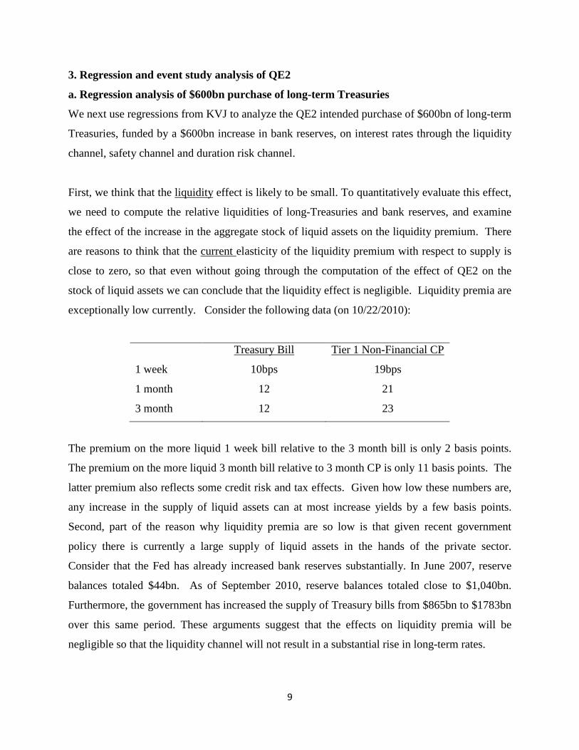
First, we think that the liquidity effect is likely to be small. To quantitatively evaluate this effect,
we need to compute the relative liquidities of long-Treasuries and bank reserves, and examine
the effect of the increase in the aggregate stock of liquid assets on the liquidity premium. There
are reasons to think that the current elasticity of the liquidity premium with respect to supply is
close to zero, so that even without going through the computation of the effect of QE2 on the
stock of liquid assets we can conclude that the liquidity effect is negligible. Liquidity premia are
exceptionally low currently. Consider the following data (on 10/22/2010):
Treasury Bill Tier 1 Non-Financial CP
1 week 10bps 19bps
1 month 12 21
3 month 12 23
The premium on the more liquid 1 week bill relative to the 3 month bill is only 2 basis points.
The premium on the more liquid 3 month bill relative to 3 month CP is only 11 basis points. The
latter premium also reflects some credit risk and tax effects. Given how low these numbers are,
any increase in the supply of liquid assets can at most increase yields by a few basis points.
Second, part of the reason why liquidity premia are so low is that given recent government
policy there is currently a large supply of liquid assets in the hands of the private sector.
Consider that the Fed has already increased bank reserves substantially. In June 2007, reserve
balances totaled $44bn. As of September 2010, reserve balances totaled close to $1,040bn.
Furthermore, the government has increased the supply of Treasury bills from $865bn to $1783bn
over this same period. These arguments suggest that the effects on liquidity premia will be
negligible so that the liquidity channel will not result in a substantial rise in long-term rates.

10
Next, consider the safety effect. With a $600bn decrease in Treasury supply, investors will have
to make do with less long-term safe assets, and hence drive up the safety premium. Table III,
column (2) of KVJ estimates the size of this safety effect. The regression is,
Baa-Aaa spread = controls + β log(Debt>10yr Maturity)
where, log(Debt>10yr Maturity) is instrumented by(Debt/GDP), (Debt/GDP)2, and
(Debt/GDP)3. The Baa-Aaa spread is the spread between two similarly liquid (or illiquid) assets,
but with a large difference in relative safety. Baas have approximately a 10% probability of
default over 10 years, while Aaas have a 1% probability of default. The regressor is long-term
Treasury supply instrumented by the total supply of Treasuries. As we explain in our paper, it is
important to instrument the long-term Treasury supply to provide an accurate estimate of β
because the maturity structure of government debt may be endogenous.
The β estimate, based on annual data from 1926 to 2008, is 0.31 (t-stat = -2.40). As of
September 2010, there was $847bn of long-term Treasury bonds outstanding. The Fed intends to
purchase $600bn of Treasuries, with maturities ranging from 2 years to 30 years. The maturity
breakdown in the intended purchases implies an average duration of the purchase of 5.5 years.
We therefore convert the $600bn purchase into $373bn of 10-year equivalents. Thus, with a
purchase of $373bn of long-term bonds, there will be $473bn left in the hands of the private
sector. Evaluating this change based on the β estimate gives an expected fall in Aaa rates of 18
basis points. Both Agency bonds and Treasury bonds are safer than Aaa corporate bonds. Thus,
we expect that the fall in these rates will be somewhat higher than the 18 basis points. How
much more? As a lower bound, if we extrapolate from the fact the difference in default
probabilities between the Baa and Aaa bonds of 9% is responsible for 18 basis points of safety
premium, then we compute that the fall in a bond with zero default risk will be 20 basis points.
This is probably an underestimate because we think the effects are non-linear near zero default
risk.
Note also that it is unlikely that the elasticity of the safety premium on long-term assets is
currently close to zero (as we argue for the liquidity premium, and is likely true for a safety

11
premium on short-term safe assets). As of 10/22/2010, the spread between Baa rates and Aaa
rates was 107 bps and the spread between Aaa rates and the 20 year Treasury bond was 111 bps.
Averages for 1919-2008 are: Baa-Aaa=118 bps and Aaa-Treasury=81 bps. Thus the current
premia are large and similar to historical averages. In addition, long-term Treasury bonds (bonds
with maturities greater than 10 years) totaled $547bn in June 2007 and $847bn in September
2010. Thus, the supply increase in long-term safe assets is modest. Indeed, if one considers that
the number of Aaa credits has also fallen over the last 3 years, it is possible that the supply of
long-term safe assets is largely unchanged.
Last consider the duration risk effect. In QE1, we estimated that the duration risk effect totaled
41 basis points. As noted above, we expect this effect to be dampened in QE2 given that we are
no longer in a period of heightened risk aversion. Here is a rough estimate of how much less:
We noted that the safety effect, which is also driven by an aversion to risky assets, drove a 123
basis point effect during QE1 – roughly 3X more than the duration effect. We have computed
that the safety effect based on average conditions is 20 basis points. If the duration effect is one-
third of this effect, then we estimate that the duration effect will drive a 6.5 basis point fall in all
long-term bond yields. With a 20 bps safety effect, a small liquidity effect and a 6.5 bps duration
risk premium effect, the regression approach predicts that QE2 should result in a fall in Treasury
yields of 26.5 basis points, in total. As for agency MBS and household mortgage rates, our
evidence suggests that historically agency MBS and mortgage rates behave like Baa bonds in
response to changes in Treasury supply, suggesting small effects of the policy on MBS yields,
given the modest size of the duration risk premium effect.
b. Event study analysis of QE2
We next analyze the actual effects on long-term interest rates of announcements surrounding the
QE2 program. The first widespread market-knowledge of the form and quantity of QE2 can
probably be traced to Chairman Bernanke’s speech Jackson Hole on 8/27/2010.8
8 http://www.federalreserve.gov/newsevents/speech/bernanke20100827a.htm
The FOMC
statement on 11/3/2010 indicated that the Fed intends to purchase $600 billion of longer-term
Treasury securities by the end of the second quarter of 2011. We thus analyze the period from
8/26 to 11/2 to determine the effect of the (anticipated) Treasury purchases on long-term interest

12
rates. [The next version of the paper will update the data to include 11/3, the date of the Fed's
announcements about QE2. Rates did not move much on 11/3, since the $600B size of QE2 was
roughly in line with market expectations, see e.g. Financial Times commentary at
http://blogs.ft.com/gavyndavies/2010/11/03/qe2-is-about-asset-prices-not-the-economy/.]
Table 2. Changes in various yields and derivatives prices on QE2 event dates (in basis points)
For the full period, most nominal interest rates rise rather than fall, indicating that other market
developments swamp the QE2 effects. In the second line of the table we focus on a subset of
dates where there is likely news about QE2. The identification is based on whether or not the
absolute value of the Aaa-Treasury spread moved at least 4 basis points. We adopt this
identification because our analysis in KVJ shows that changes in the supply of long-maturity
Treasuries will affect this spread via Treasury convenience yield changes. Thus, we infer that
large moves (up or down) in the Aaa-Treasury spread are likely to be associated with news
(positive or negative) about the size or likelihood of implementation of QE2. Importantly, the
outcome variable of interest is still the CDS-adjusted Baa rate, so the identification does not
induce any mechanical effect. Furthermore, none of the 10 days we identify as QE2 news days
experienced a substantial (greater than 4 bps) change the investment grade CDS rate and a
change in the Aaa-Treasury spread in the same direction, supporting our conjecture that the
changes in Aaa-Treasury spreads really do indicate news about QE2.
The effects on nominal yields are in line with our previous analysis. The credit-adjusted change
in the Baa rate indicates a fall of 10 basis points. This effect is a pure duration risk-premium

13
effect. The 10 year Treasury rate falls by 25 basis points, which is close to the three-to-one ratio
from the prior analysis. The Agency yields fall by 27 basis points, consistent with our prediction
for effects on long-term safe assets. These numbers are in line with the 26.5 basis points we
estimated from the regression analysis. As for inflation, the inflation swap rate indicate
essentially no impact of QE2 on expected inflation. Overall, we estimate that QE2 reduces real,
default-adjusted Baa corporate rates by only 9 bps. This is much smaller than the 24 bps impact
of QE2 on real Treasury rates due to an impact of QE2 on the Treasury convenience
(safety/liquidity) yield. We estimate the change in the Treasury convenience yield to be 15 bps
(last column of Table 2).
4. Conclusion
We document a significant lowering of the nominal interest rates on Treasuries and Agencies as
a result of QE1 and QE2. However, we show that QE1 and (announced) QE2 purchases of long-
term Treasuries (and other long-term bonds in the case of QE1) has had a smaller effect on
nominal Baa rates, rates more relevant for corporate borrowing. For QE2, we predict a similarly
small effect on nominal Agency MBS rates or household mortgage rates [numbers to be added in
next version] since QE2 purchases target only Treasury bonds. As for inflation, QE1 generated a
substantial increase in expected inflation, resulting in large reductions in real rates, whereas QE2
has had little impact on expected inflation. Our findings indicate that the measured impact of
quantitative easing is crucially dependent on focusing on the most policy relevant rates (Baa
rates and household mortgage rates more than Treasury rates). Methodologically, we show that
derivatives prices from credit-default swaps and inflation swaps can provide central inputs to
macroeconomic policy assessment. We furthermore propose a market-based measure of event
dates for a given policy. This identification approach is useful for assessing policies such as QE2
for which market assessment about size and likelihood of implementation changed gradually
without any firm announcement from the Fed until November 3.

14
References D'Amico, Stefania, and Thomas B. King, 2010, "Flow and Stock Effects of Large-Scale Treasury Purchases," Finance and Economics Discussion Series 2010-52. Washington: Board of Governors of the Federal Reserve System, September. Fleckenstein, Matthias, Francis A. Longstaff, and Hanno Lustig, 2010, "Why does the Treasury Issue TIPS? The TIPS-Treasury Bond Puzzle", working paper, UCLA. Gabaix, Xavier, Arvind Krishnamurthy and Olivier Vigneron, 2007, "Limits of Arbitrage: Theory and Evidence from the Mortgage-Backed Securities Market," Journal of Finance, 62(2), pages 557-595, 04. Gagnon, Joseph, Matthew Raskin, Julie Remache, and Brian Sack, "Large-Scale Asset Purchases by the Federal Reserve: Did They Work?" Federal Reserve Bank of New York Staff Report no. 441, March 2010. Greenwood, Robin and Dimitri Vayanos, 2010, “Bond Supply and Excess Bond Return,” working paper, LSE. Hamilton, James D., and Jing Wu, 2010, "The Effectiveness of Alternative Monetary Policy Tools in a Zero Lower Bound Environment," working paper. San Diego: University of California, San Diego. Krishnamurthy, Arvind and Annette-Vissing Jorgensen, 2010, “The Aggregate Demand for Treasury Debt,” working paper, Northwestern University. Longstaff, Francis A., Sanjay Mithal and Eric Neis, 2005, "Corporate Yields Spreads: Default Risk or Liquidity? New Evidence from the Credit-Default Swap Market," Journal of Finance, 60(5), pages 2213-2254.

The Aggregate Demand for Treasury Debt
Arvind Krishnamurthy Annette Vissing-Jorgensen∗
May 12, 2010
Abstract
Investors value the liquidity and safety of U.S. Treasury bonds. We document this by showing that
changes in Treasury supply have large effects on a variety of yield spreads. As a result, Treasury yields
are reduced by 72 basis points, on average over the period from 1926-2008. The low yield on Treasuries
due to their extreme safety and liquidity suggests that Treasuries in important respects are similar to
money. Evidence from quantities supports this idea. When the supply of Treasuries falls, reducing the
overall supply of liquid and safe assets, the supply of bank-issued money rises.
∗Respectively: Northwestern University and NBER; Northwestern University, NBER and CEPR. We thank Ricardo Ca-
ballero, Mike Chernov, Chris Downing, Ken Garbade, Lorenzo Garlappi, Robin Greenwood, Dimitri Vayanos, Sam Hanson,
Mike Johannes, Bob McDonald, Monika Piazzesi, Sergio Rebelo, Suresh Sundaresan, Pierre-Olivier Weill, Tan Wang, Francisco
Palomino, Clemens Sialm, Gerard Hoberg, Henning Bohn, and participants at talks at UCLA, University of Chicago, Columbia
University, Michigan State University, Duke-UNC Asset Pricing conference, Fed Board of Governors, University of Michigan
Mitsui Life Symposium on Financial Markets, LSE-PWC conference, MIT, Moody’s-KMV, NBER AP meeting, NBER ME
meeting, NBER EFG meeting, UBC Winter Finance Conference, Northwestern University, NY Fed, University of Texas-Austin,
University of South Carolina, Queen’s University and the WFA for comments. Josh Davis, Chang Joo Lee, and Byron Scott
provided research assistance. We thank Moody’s KMV for providing their Expected Default Frequency data, Michael Fleming
for data on P2 rated commercial paper, and Henning Bohn for Debt/GDP data.

1 Introduction
Money, such as currency or checking accounts, offers a low rate of return relative to other assets. The reasons
behind this phenomenon are well understood. Money is (1) a medium of exchange for buying goods and
services, (2) of high liquidity, and (3) of extremely high safety in the sense of offering absolute security of
nominal repayment. Investors value these attributes of money and drive down the yield on money relative
to other assets.
We argue that Treasury bonds have some of the same features as money, namely (2) and (3), and
that this drives down the yield on Treasuries relative to assets that do not to the same extent share these
features. Figure 1A provides vivid evidence for this assertion. The figure graphs the yield spread between
Aaa rated corporate bonds and Treasury securities against the US government Debt-to-GDP ratio (i.e. the
ratio of the market value of publicly held US government debt to US GDP). The figure reflects a Treasury
demand function, akin to a money demand function. When the supply of Treasuries is low, the value that
investors assign to the liquidity and safety attributes offered by Treasuries (referred to below as the Treasury
convenience yield) is high. As a result the yield on Treasuries is low relative to the yield on the Aaa corporate
bonds which offer less liquidity and safety. The opposite applies when the supply of Treasuries is high. We
present detailed econometric evidence of the relation reflected in Figure 1 using several alternative yield
spread measures and controlling for corporate bond default risk.
The evidence in Figure 1 shows that Treasuries offer unique attributes that are valued by investors, but
does not identify the attributes. We further show that Treasuries share features (2) and (3) with money
in two ways. First, we examine the yield spread between a pair of assets which are different only in terms
of their liquidity, as well as the yield spread between a pair of assets which are different only in terms of
their safety. Under the hypothesis that liquidity/safety are priced attributes, the yield spread between these
pairs of assets should reflect the equilibrium price of liquidity/safety. We show that changes in Treasury
supply affect each of these yield spreads. The results indicate that Treasuries offer liquidity and safety so
that changes in the supply of Treasuries separately change the equilibrium price of liquidity and safety.
The second type of evidence that Treasuries share (2) and (3) with money relates the quantity of money
to the quantity of Treasuries. We show that when the supply of Treasuries falls, the supply of bank-issued
money (specifically, M2 minus M1) which offers (2) and (3), rises. We show that the channel underlying this
response is that a reduction in the supply of Treasuries increases the prices of liquidity and safety, lowering
the yield on bank deposits, and inducing the banking sector to issue more deposits.
These findings suggest that investors value liquidity and safety when pricing assets. We compute that
the value investors have paid on average over our main sample from 1926 to 2008 for the liquidity and safety
attributes of Treasuries is 72 basis points per year of which 46 basis points is for liquidity and 26 basis points
for safety. The government collects seignorage from the liquidity and safety attributes of Treasuries and we
1
compute that the government saves interest costs of 0.25% of GDP per year because of investors’ demand
for Treasuries. This figure is comparable in magnitude to the traditional notion of seignorage, which stems
from the public’s willingness to hold fiat money at zero interest. We compute that the latter seignorage is
around 0.24% of GDP per year.
In addition to their implications for asset pricing and seignorage, our findings have implications for the
demand for money. First, since Treasuries share some of the attributes of money, appropriately constructed
“money” aggregates should include the supply of Treasuries. Second, the demand for money stems from
demand for liquidity, safety, and a medium-of-exchange. It is likely that there is independent variation in
the demand and supply of each of these attributes. For example, during a financial crisis, the demand for
liquidity and safety in particular may rise. On the other hand, the extant literature on money demand
assumes that money reflects the price of a single attribute. We discuss how to use the yields on Treasuries
as well as other safe/liquid assets to recover the underlying demands for the different attributes of money.
These findings help shed light on sources of instability in estimates of the money demand function (see
Goldfeld and Sichel, 1990).
Finally, our findings imply that Treasury interest rates are not an appropriate benchmark for “riskless”
rates. Cost of capital computations using the CAPM should use a higher riskless rate than the Treasury rate
– a company with a beta of zero cannot raise funds at the Treasury rate. In addition, our results suggest
that the equity premium measured relative to Treasury rates will partly be driven by the liquidity and safety
of Treasuries and thus that these Treasury properties are partially responsible for the high equity premium.
Relation to Literature
Our finding of a significant non-default component in the corporate bond spread is consistent with some
recent papers in the corporate bond pricing literature (see Collin-Dufresne, Goldstein, and Martin (2001)
and Longstaff, Mithal, and Neis (2005)). Duffie and Singleton (1997), Grinblatt (2001), Liu, Longstaff,
and Mandell (2004), and Feldhutter and Lando (2005) argue for a significant non-default component in the
interest rate swap spread (the spread between the fixed rate in a fixed-for-floating interest rate swap contract
and the Treasury rate). Papers in the prior literature use information from the corporate bond market and
credit default swaps to estimate the default component of interest rate spreads, and label the residual as a
non-default component. Compared to the prior literature, the novelty of our work is to offer direct evidence
of the existence of a non-default component by documenting that the amount of Treasuries outstanding is
a key driver of the non-default component of the corporate bond spread (a similar relation holds for the
interest rate swap spread but we do not emphasize that here since swap rates are only available for a fairly
short period, starting in 1987).1
1Some of the papers in the prior literature show that the non-default component is related to the specialness of particular
Treasury securities. A particular Treasury bond is “special” if the cost of borrowing the bond in the repurchase market exceeds
2

We are aware of only a few papers in the literature that have noted a correlation between the supply of
government debt and interest rate spreads. Cortes (2003) documents a correlation between the US Debt/GDP
ratio and swap spreads over a period from 1994 to 2003. Longstaff (2004) documents a correlation between
the supply of Treasury debt and the spread between Refcorp bonds and Treasury bonds over a period from
1991 to 2001. Friedman and Kuttner (1998) show a correlation between the commercial paper to Treasury
Bill spread and the relative supply of these assets over the period 1975 to 1996.2 Relative to these papers we
study a much longer sample, provide a theoretical basis to study the relation, use several approaches to rule
out that the relation could be driven by time-varying default risk, decompose the Treasury convenience yield
into a liquidity and safety component, and show the similarity between money and Treasuries by showing
that private sector money supply reacts to Treasury supply.
There is a closely related literature that seeks to examine whether the relative supplies of long and short-
term Treasury debt has an effect on the term structure of Treasury yields. Early work in this literature was
motivated by the 1962-64 “operation twist,” where the government tried to flatten the term structure by
shortening the average maturity of government debt (see for example Modigliani and Sutch, 1966). More
recently, Reinhart and Sack (2000) show that the projected government deficit is positively related to the
slope of the Treasury yield curve, suggesting that this is evidence of a supply effect. More systematic evidence
of a relative supply effect is provided in Greenwood and Vayanos (2010), who examine data from 1952 to
2005 and show that relative supply of long and short Treasuries is related to the slope of the yield curve as
well as the excess return on long-term Treasuries over short-term Treasuries. These papers suggest that the
demand for Treasury attributes varies by maturity, and are complementary to our study.
In macroeconomics, there is a large literature exploring the Ricardian equivalence proposition (Barro,
1974), that the financing choices of the government used to fund a given stream of government expenditures
is irrelevant for equilibrium quantities and prices. One implication of the Ricardian equivalence proposition
is that the size of government debt has no causal effect on interest rates. Despite a large amount of research
devoted to studying this topic, there is yet no clear consensus on the effects of debt on interest rates (see, for
example, the survey by Elmendorf and Mankiw (1999)). Barro (1987), Evans (1986) and Plosser (1986) find
little or no effect of government debt on interest rates. Focusing on forward Treasury rates and projected
future Debt/GDP levels, Laubach (2007) reports a 3 − 4 bps effect per one percentage point increase in
projected Debt/GDP. We provide evidence that the stock of government debt affects the interest rates
that of other Treasury bonds with similar maturity and cash-flow characteristics. Specialness leads to the yield on the special
Treasury bond to fall below comparable Treasury bonds. See Krishnamurthy (2002) for further discussion of specialness. We
show that the entire Treasury market is “special” relative to other asset markets, and not just that one Treasury is special
relative to another Treasury.2There is a related fixed income literature documenting that the auctioned amount of a specific Treasury security affects
the value of this security relative to other Treasury securities (Krishnamurthy (2002) and Sundaresan and Wang (2006) are
examples). We show an effect relative to non-Treasury securities.
3

on government bonds. But it is important to note that the effect we identify is on the spread between
government interest rates and corporate interest rates. It is possible that Ricardian equivalence fails in a
way that government debt has an effect on the general level of interest rates, both corporate and government.
Since we focus on spreads, we are unable to isolate such an effect. On the other hand, because we focus
on spreads we can be certain that the effect we identify on government interest rates is over and above any
possible effects of government debt on the general level of interest rates. From an empirical standpoint,
the advantage of focusing on spreads rather than the level of interest rates is that the spread measure is
unaffected by other shocks (such as changes in expected inflation) that affect the level of interest rates and
complicate inference. We also bypass endogeneity issues stemming from government behavior, since it is
unlikely that the government chooses debt levels based on the corporate bond spread.
This paper is laid out as follows. The next section lays out a theoretical framework to relate the demand
for the attributes offered by Treasuries to the price of Treasuries relative to other assets. The section develops
a series of predictions of the theory. We test each of the theoretical predictions in Section 3. In Section 4
we discuss the implications of our findings for a number of important issues in macroeconomics and finance.
The paper also includes an appendix providing details on the data construction as well as mathematical
derivations.
2 Theoretical Framework
We articulate our theory by modifying a standard representative agent asset-pricing model to include a term
whereby agents derive utility directly from holdings of a “convenience” asset. The modification is along
the lines of Sidrauski (1967) and Lucas (2000) who consider models where agents derive utility from their
holdings of money. We consider a representative agent who maximizes,
E
∞∑
t=1
βtu(Ct) (1)
where Ct is the agent’s consumption at date t. We introduce utility from holdings of a convenient asset as
follows. Suppose that the consumption of Ct is the sum of an endowment of ct plus “convenience” benefits:
Ct = ct + ν(θAt , GDPt; ξt). (2)
The benefits are a function of the holdings of convenience assets, θAt . One example which we elaborate on
below is that the function ν(·) captures the notion that holding more Treasury securities reduce costs that
would otherwise be incurred by transacting in a less liquid security such as corporate bonds.3 The argument
3To be more precise, we can define Ct = ct−cost(θAt ,GDPt ; ξt), where the function cost(·) reflects costs that will be incurred
by holding less liquid securities. By holding more Treasuries, these costs are reduced. This is just a renormalization relative to
our defining a benefit function ν(·) that is increasing in θAt . The important aspect of the modeling is that dCt/dθA
t > 0.
4

θAt is the market value of the agent’s real holdings of convenience assets and include both Treasuries, θT
t ,
and any other private sector assets, θPt , that provide services similar to Treasuries:
θAt = θT
t + kP θPt . (3)
The constant kP measures the convenience services provided by the private sector assets relative to Treasuries.
The term ξt in the convenience function is a preference shock that affects how much utility is derived from
convenience assets. An example of such a shock is a “flight-to-quality” as during a financial crisis, where
investors may temporarily increase their valuation of convenient assets such as Treasuries.
We assume that the convenience function is homogeneous of degree one in GDPt and θAt . This captures
the idea that liquidity benefits double if both income and convenience assets double. Thus define,
v
(
θAt
GDPt; ξt
)
GDPt ≡ ν(θAt , GDPt; ξt). (4)
We assume that the convenience function is increasing inθA
t
GDPt, but the marginal convenience benefit is
decreasing inθA
t
GDPtand has the property lim θA
tGDPt
→∞
v′(θA
t
GDPt; ξt) = 0. That is, holding more convenience
assets reduces the marginal value of an extra unit of convenient assets. Furthermore, this marginal value
approaches zero if the agent is holding a large amount of convenient assets.
Let us next consider what underlies our reduced form convenience function v(·). In the monetary eco-
nomics literature, the convenience of money stems from three attributes: its role as a medium of exchange,
its superior liquidity, and its safety in the sense of retaining a certain nominal value. The demand for these
attributes drives the low yield on money relative to other assets. While Treasuries do not have the medium
of exchange attribute, we argue that they share the liquidity and safety attributes. Papers such as Aiyagari
and Gertler (1991), Heaton and Lucas (1996), Vayanos and Vila (1998), and Rocheteau (2009) show how the
superior liquidity of an asset will lead investors to pay a higher price for that asset. Under these theories,
an increase in the holding of liquid assets will lower the marginal liquidity service provided by any liquid
asset. That is, our earlier assumption that the marginal convenience, v′(·), is decreasing inθA
t
GDPtis a natural
outcome of these models. We refer to these theories as describing a liquidity attribute.
The liquidity models we have cited are all heterogeneous agent models rather than homogeneous repre-
sentative agent models. These models all have two classes of agents where one class trades with the other,
incurring transaction costs when such trade involves illiquid assets. In equilibrium, the prices of liquid assets
carry a premium over less liquid assets, producing a liquidity function resembling v(·). It is important to
keep in mind that while we introduce v(·) in a representative agent model, this reduced form function is
motivated by an underlying theoretical model with heterogeneous agents.
A second benefit of Treasuries is that they are widely believed to provide absolute certainty of nominal
repayment. Under some theories, this safety attribute can drive a convenience yield that is declining in the
5

supply of safe assets. Suppose that some investors face costs of understanding investment in risky assets,
as in the literature on the limited participation of investors in the stock market (Vissing-Jorgensen, 2003).
These investors will have a unique demand for riskless assets, driving up the price of riskless assets. The
existing literature has shown that participation costs can explain why risk premia on stocks may be high and
why interest rates on riskless assets may be low. In addition, in many limited participation models expanding
the stock of riskless assets reduces risk premia and raises riskless rates (see Gomes and Michaelides, 2008).
Another explanation for safety demand stems from the use of Treasuries as collateral in many financial
transactions. Gorton (2010) notes that there is a substantial demand for collateral for purposes of mitigating
counterparty risk in derivatives and settlement systems. The collateral in these transactions is required to
be extremely safe, thus also driving the demand for a safety attribute. Bansal and Coleman (1996) argue
that commercial banks and money market funds use Treasuries to back checkable deposits. Treasuries thus
inherit some of the medium-of-exchange convenience of money, lowering the yield on Treasuries. In this
explanation, it is again the safety of Treasuries that makes them good backing for checking accounts. We
will offer empirical evidence that the safety attribute of Treasuries is one of the drivers of the convenience
yield. However, we will not distinguish further on whether the underlying driver of safety demand is due to
limited participation, collateral, or the check-backing explanations.
Two points are worth noting. First, since long-term Treasury bonds carry interest rate risk it is unlikely
that the explanations offered in the previous paragraph also apply to long-term bonds. For this reason, we
refer to this Treasury property as “short-term” safety. In addition, this safety explanation is distinct from
that suggested by any of the standard representative agent model explanations of high risk premia in asset
markets. This literature has demonstrated how altering the preferences of a representative agent to feature
extreme forms of risk aversion can produce low riskless interest rates and high risk premia. However, the
quantity of convenient assets is unrelated to asset prices in the representative agent model. One needs a
richer model with heterogeneity and/or frictions, along the lines of the literature cited above, to rationalize
the quantity effect. The quantity-price relationship is at the heart of our study. Another way to think about
how safety demand works is that the relation between price and default risk is very steep near zero-default-
risk. Furthermore, the slope of this curve near zero-default-risk decreases in Treasury supply. This latter
prediction generates a negative relation between the corporate-Treasury bond spread and Treasury supply.
There are also theories for why safe nominal long-term payoffs may be uniquely valued. Greenwood
and Vayanos (2010) suggest that investors such as defined benefit pension funds have a special demand for
certain long-term payoffs to back long-term nominal obligations. The same motive may apply to insurance
companies that write long-term policies. Chalmers (1998) describes how long-term Treasury bonds are
posted as collateral by municipalities to secure their own borrowings. Broadly, this explanation is similar
to the preferred habitat hypothesis of the term structure of interest rates (Modigliani and Sutch, 1966),
6

under which investors are hypothesized to prefer certain maturities of bonds. We refer to these theories as
a describing a long-term safety attribute.
We can represent these different theoretical rationales for convenience in our specification of v(·). Denote
θT,longt as the stock of long-term Treasury bonds, and θT,short
t as the stock of short-term Treasuries (θTt =
θT,longt + θT,short
t ). Also define θP,liqt as the stock of non-Treasury liquid assets, θP,short−safe
t as the stock
of non-Treasury short-term safe assets, and θP,long−safet as the stock of non-Treasury long-term safe assets.
Suppose that total convenience on short-term Treasuries can be written as the sum of two convenience
components:
vT,short(·) = vliq
(
θTt + kliqθP,liq
t
GDPt; ξliq
t
)
+ vshort−safe
(
θT,shortt + kshort−safeθP,short−safe
t
GDPt; ξshort−safe
t
)
.
(5)
Similarly, we can specify the convenience on long-term Treasuries as
vT,long(·) = vliq
(
θTt + kliqθP,liq
t
GDPt; ξliq
t
)
+ vlong−safe
(
θT,longt + klong−safeθP,long−safe
t GDPt; ξlong−safet
)
.
(6)
The constants, kliq , kshort−safe and klong−safe, measure the convenience that the private sector assets offer
relative to Treasuries.
Our specification emphasizes that the safety attributes may differ across short and long-term assets
and thus lead to a difference in convenience value in long-term assets relative to short-term assets. In
contrast, our specification assumes that both long and short-term Treasuries offer equal liquidity services.
The empirical literature has documented the existence of significant liquidity premia on both long-term
Treasuries (Krishnamurthy, 2002) and short-term Treasuries (Amihud and Mendelsen, 1991). We are making
the somewhat stronger assumption that long and short-term Treasuries are equally liquid (see Fleming, 2003,
for more on this point).
2.1 Spreads and Supply
We derive pricing expressions for short and long-term bonds based on these different specifications of conve-
nience. As we describe below, decomposing the convenience in the manner above also yields empirical tests
of the existence of priced safety and liquidity attributes. Before describing these tests, let us turn to asset
pricing. We initially derive predictions of the convenience yield theory which do not distinguish between the
liquidity and safety motives. We then turn to predictions implied by each of these separate motives. In terms
of the framework above, our initial set of predictions implicitly assume that both vT,long and vT,short are
only functions of θTt (as opposed to functions of both total Treasury supply and short or long-term Treasury
supply). This will be the case if long and short Treasury supply moves in parallel (and if the demand shocks
are perfectly correlated), or if only a liquidity motive is present. We relax this assumption later.
7

Denote the price level at date t as Qt. If the agent buys a zero coupon Treasury bond for a nominal price
P Tt , his real holdings θA
t rises byPT
t
Qt.4 The first order condition for Treasury bond holdings is then,
−P T
t
Qtu′(Ct) + βEt
[
P Tt+1
Qt+1u′(Ct+1)
]
+P T
t
Qtv′(θA
t /GDPt, ξt)u′(Ct) = 0 (7)
Define the pricing kernel for nominal payoffs as,
Mt+1 = βu′(Ct+1)
u′(Ct)
Qt
Qt+1, (8)
so that,
P Tt = Et[Mt+1P
Tt+1] + P T
t v′(θAt /GDPt; ξt) ⇒ P T
t =Et[Mt+1P
Tt+1]
1 − v′(θAt /GDPt; ξt)
. (9)
This expression indicates that a positive marginal value of convenience, v′(·), raises the price of Treasuries,
P Tt .
Let us next derive pricing expressions for a zero-coupon corporate bond that offers no convenience services.
Suppose that the corporate bond may default next period with probability λt and in default pays 1− Lt+1,
where Lt+1 measures the amount of losses suffered in default. If the bond does not default, it is worth P Ct+1.
Then, since the bond offers no convenience, its price satisfies
P Ct = λtEt[Mt+1(1 − Lt+1)|Default] + (1 − λt)Et[Mt+1P
Ct+1|No Default] (10)
In our empirical work we estimate the convenience demand v′(·) by relating θTt to different measures of
the price difference between P Ct and P T
t . There are three price measures we focus on: short-maturity yield
spreads between corporate and Treasury bonds, long-maturity yield spreads, and excess returns of corporate
bonds over Treasury bonds. We now derive expressions for each of these price measures and compare them.
For simplicity, we focus our derivations on zero-coupon bonds and continously compounded yields.
Consider first the case of one period bonds. For such bonds, P Ct+1 = P T
t+1 = 1. Then,
e−iTt = P T
t =Et[Mt+1P
Tt+1]
1 − v′(θAt /GDPt; ξt)
≈ ev′(θAt /GDPt;ξt)Et[Mt+1] (11)
For the corporate bond, define L̃t+1 as a random variable that is equal to zero if there is no default, and
equal to Lt+1 if there is default. Then,
e−iCt = P C
t = Et[Mt+1]−Et[Mt+1]Et[L̃t+1]−covt[Mt+1, L̃t+1] ≈ e−λtEt[Lt+1]−covt[Mt+1,L̃t+1]/Et [Mt+1]Et[Mt+1]
We thus have the following prediction:
4We deriving pricing expressions for zero-coupon Treasury and corporate bonds. In our empirical work, we examine coupon
bonds and assume that the impact of Treasury supply on coupon bond spreads are qualitatively similar.
8

Prediction 1 (Impact of Treasury supply on short-term spreads)
The one-period yield spread between corporate and Treasury bonds is related to the stock of Treasuries as
follows:
St,1 ≡ iCt − iTt = v′(
θTt + kP θP
t
GDPt; ξt
)
+ λtEt[Lt+1] + covt[Mt+1, L̃t+1]/Et[Mt+1]. (12)
The yield spread reflects the sum of three terms: the convenience yield on Treasuries, the expected default
rate on the corporate bond, and a risk premium associated with the covariance between default and the pricing
kernel. Assuming that v′′(·) < 0, St,1 is declining in θTt + kP θP
t . Consider next the relationship between St,1
and θTt . Project θP
t linearly on θTt , so that θP
t = a0 + a1θTt + error, where the error is uncorrelated with θT
t .
Then θTt + kP θP
t = kP a0 +(1 + kP a1)θTt + kP error. If 1 + kP a1 > 0, then St,1 is declining in θT
t . The latter
condition will be satisfied if a1 > −1/kP , i.e. unless the private sector reduces its supply of substitutes by
more (in effective terms, kP θPt ) than the increase in the Treasury supply.
We verify the prediction of the convenience model that an increase in θTt causes the yield spread to fall. Our
regressions of the yield spread on θTt recover v′(·)
(
1 + kP ∂θPt
∂θTt
)
rather than v′(·) because of private sector
reaction. In order to recover v′(·), we further need knowledge of kP and∂θP
t
∂θTt
. We do not explore that in this
paper because for most questions of interest, it is more important to know v′(·)(
1 + kP ∂θPt
∂θTt
)
rather than
v′(·).
Note that it is possible that Treasury supply or private sector supply reacts accommodating to demand
shocks (ξt) or to increases in corporate default risk. This will bias the relation between spreads and Treasury
supply towards finding a positive relation, the opposite of the causal negative relation from Treasury supply
to spreads. However, we view it as unlikely that overall Treasury supply reacts substantially to demand
shocks or changes in the risk of corporate bonds. The more plausible reaction involves the private sector
supply or the government’s supply of particular maturities.
Let us next consider multi-period bonds. Define the τ period yields on corporate and Treasury bonds as,
iTt,τ = −1
τln P T
t and, iCt,τ = −1
τln P C
t . (13)
The spread between these bonds is St,τ = iCt,τ − iTt,τ .
Consider again the derivation for corporate bonds. Our derivation for multi-period bonds closely follows
Duffie and Singleton (1999), reflecting the standard practice in the corporate bond pricing literature. Suppose
that the event of default or no-default is non-systematic (i.e. uncorrelated with Mt+1). Then, we can drop
the conditioning on default/no-default and rewrite (10) as,
P Ct = Et[Mt+1
(
λt(1 − Lt+1) + (1 − λt)PCt+1
)
] (14)
Assume that we can write the expected present value of the payment in default as,
Et[Mt+1(1 − Lt+1)] = Et[Mt+1PCt+1](1 − Dt) (15)
9

for a suitable process Dt.5 This is Duffie and Singleton’s “recovery of market value” assumption (RMV).
Then,
P Ct = (λt(1 − Dt) + (1 − λt))Et[Mt+1P
Ct+1] ≈ e−λtDtEt[Mt+1P
Ct+1]. (16)
Note that the term P Ct+1 is a function of Dt+1 and λt+1, which embody changes in future default expectations
such as downgrades. For high-grade corporate bonds, which are the focus our study, almost all of the default-
related risk is of this form rather than in terms of the bonds defaulting between t and t + 1. In our setup,
the latter default-related risk may be correlated with Mt+1 and carry a risk premium. Thus, our restriction
that the default event in the next period is non-sytematic is not a substantively important restriction, but
does help to simplify our pricing expressions.
Prediction 2 (Impact of Treasury supply on long-term spreads)
The yield spread between τ -period corporate and Treasury bonds is related to the stock of Treasuries as follows,
St,τ =
t+τ−1∑
j=t
1
τEt[v
′(θAj /GDPj; ξj)] +
t+τ−1∑
j=t
1
τEt[λjDj ] −
t+τ−1∑
j=t
1
τcovt(mj+1, R̃j+1) (17)
where, mj+1 = logMj+1 (= log βu′(Cj+1)u′(Cj)
Qj
Qj+1), is the log pricing kernel, and R̃j+1 is the one-period excess
return of corporate bonds over Treasury bonds. As long as θAj increases with θT
j , increases in Treasury supply
lower the spread, St,τ .
The derivation of this spread expression is in the Appendix. The derivation assumes that all relevant
variables, including mt and changes in the corporate and Treasury bond yields, are normally distributed.
The spread reflects three terms: (1) the expected average convenience benefit over the next τ periods;
(2) the expected average amount of default; and (3) a risk premium that depends on the covariance between
the pricing kernel and the excess return on corporate over Treasury bonds.
Let us pause and compare the short-term and long-term spread expressions. Note that shocks to both
θAt /GDPt and ξt have an impact on the short-term spread. The impact of these shocks on the long-term
spread depends on the persistence of the shocks. In the data, a flight to quality (liquidity and safety) shock
(ξt) is short-lived, and should primarily affect short-term spreads. The debt-to-GDP ratio is quite persistent
so that shocks to θAt /GDPt will have a significant impact on both short and long-term spreads. This logic
tells us that the convenience yield as embodied in the long-term spread is primarily driven by θAt /GDPt,
while variability in the short-term spread will partly be driven by ξt.6 This is an advantage of using the
5Note that in expression (15), the left-hand side expectation is conditioning on default, while the right-hand side expectation
is conditioning on no-default. However, given the assumption that the default-event is non-systematic, we can drop the
conditioning.6Here is a simple case to formalize these points. Suppose that the convenience yield function is
v′(θAt /GDPt; ξt) = b0 + b1 log(θA
t /GDPt) + logξt.
10

long-term spread and data on θAt /GDPt to estimate convenience yields. On the other hand, the corporate
bonds we use to construct the short-term spread are close to default free. The corporate bonds used in
the long-term spread carry greater default risk. Thus, the results based on the long-term spread are more
sensitive to precise controls for default risk.
The last price variable we examine is the excess return of (zero coupon) corporate bonds over Treasury
bonds. For Treasury bonds,
1 − v′(θAt /GDPt; ξt) = Et
[
Mt+1P T
t+1
P Tt
]
(18)
We consider the return on a Aaa/Aa index of corporate bonds on which default over the holding period are
exceptionally rare. Downgrades are the relevant default-related event. Thus,
1 = Et
[
Mt+1P C
t+1
P Ct
]
(19)
Prediction 3 (Impact of Treasury supply on excess returns)
The expected excess return of corporate bonds over Treasuries is related to the stock of Treasuries as follows,
Et[Mt+1R̃t+1] = v′(θAt /GDPt; ξt). (20)
We can rewrite this expression as,
Et[R̃t+1] =1
Et[Mt+1]
(
v′(θAt /GDPt; ξt) − covt(Mt+1, R̃t+1)
)
. (21)
As long as θAj increases with θT
j , an increase in θTt implies a decrease in the expected return on corporate
bonds over Treasury bonds.
Let us compare how the excess return regression compares to the yield spread regressions. The advantage
of studying returns over yields is that while time-variation in expected default affect yields such variation
does not affect expected returns. However, studying returns also has distinct disadvantages. If we take a
log-linear approximation, the excess return, R̃t+1 is approximately the change in the long-term yield spread,
−(τ −1)St+1,τ−1 + τSt,τ . We can substitute from the expression for St,τ (and St+1,τ−1) from above, and set
Here, we have written the demand shock, ξt, to enter additively in the convenience yield, and assumed a log convenience yield
function, as we do in most of our empirical tests. The short-term spread equally reflects a supply term b1 log(θAt /GDPt) and
a demand term b1 logξt. Suppose that log(θAt /GDPt) is AR(1) with coefficient ρ and that logξt is i.i.d. with mean zero. Then
it is easy to verify that the convenience yield component of the long-term spread is,
t+τ−1X
j=t
1
τEt[v
′(θAj /GDPj ; ξj)] = b0 + b1 log(θA
t /GDPt)`
1 + ρ + ρ2 + ... + ρτ−1´ 1
τ+
logξt
τ.
If we take τ = 20 years (the maturity for the long spread in our study), and ρ = 0.95 (consistent with data on the Debt-to-GDP
ratio), then the supply coefficient`
1 + ρ + ρ2 + ... + ρτ−1´
1
τis 0.64, while the demand coefficient 1/τ is 0.05.
11
λt = 0 (i.e. no defaults on the corporate bonds in the return index, over the next one period) to find R̃t+1:
R̃t+1 ≈ v′(θAt /GDPt; ξt) − covt(mt+1, R̃t+1) (22)
−
t+τ−1∑
j=t+1
(
Et+1[v′(θA
j /GDPj; ξj)] − Et[v′(θA
j /GDPj; ξj)])
−
t+τ−1∑
j=t+1
(Et+1[λjDj ] − Et[λjDj ])
+
t+τ−1∑
j=t+1
(
covt+1(mj+1 , R̃j+1) − covt(mj+1, R̃j+1))
The first line of this expression is the expected excess return. This expected return reflects the convenience
yield as well as the risk premium associated with the variability of corporate-Treasury returns. Changes in
θTt will alter the convenience yield, and hence the expected return, in a similar manner as they affect the
short-term yield spread. To estimate the convenience yield using excess return regressions, we need to control
for any time variation in the risk premium. The long-term spread regressions also require us to control for
variation in risk premia, so that in this regard these two price measures have a similar disadvantage. However,
the second, third, and fourth lines indicate the disadvantage of studying returns, namely that realized excess
returns are affected by news about the convenience benefits on Treasuries, about default and about future
risk premia. Realized returns thus could differ dramatically from expected returns, making it statistically
difficulty to detect our predicted relation between expected returns and Treasury supply. Given the pros
and cons of studying returns versus yields, we present results from both approaches in our empirical work.
2.2 Liquidity and Safety Attributes
We now reintroduce the different liquidity and safety attributes of Treasuries and consider how one can
test if these attributes are priced. Following equations (5) and (6), long and short-term assets should be
expected to have different convenience yields. To be precise, let us reconsider the short and long-term spread
expression. The short-term spread reflects liquidity and short-term safety:
St,1 = v′liq
(
θTt + kliqθP,liq
t
GDPt; ξliq
t
)
+ v′short−safe
(
θT,shortt + kshort−safeθP,short−safe
t
GDPt; ξshort−safe
t
)
+λtEt[Lt+1] + covt[Mt+1, L̃t+1]/Et[Mt+1]. (23)
The long-term spread, for large τ , reflects the expected liquidity and long-term safety attributes over the
term of the bond:
St,τ =t+τ−1∑
j=t
1
τEt
[
v′liq
(
θTj + kliqθP,liq
j
GDPj; ξP,liq
j
)
+ v′long−safe
(
θT,longj + klong−safeθP,long−safe
j
GDPj; ξlong−safe
j
)]
+
t+τ−1∑
j=t
1
τEt[λjDj] −
t+τ−1∑
j=t
1
τcovt(mj+1, R̃j+1) (24)
12

There are a few approaches to test for the existence of separate priced attributes. If we can treat variation
in the supply of long and short-term Treasuries as exogenous to other shocks, then a way of identifying the
short and long-term safety attributes is to ask whether an increase in θT,shortt has a larger effect on the
short-term spread than an increase in θT,longt does, and whether an increase in θT,long
t has a larger effect
on the long-term spread than an increase in θT,shortt does. This approach, although not stated in terms
of safety attributes, is taken by Greenwood and Vayanos (2010) in their study of government maturity
structure and the slope of the yield curve. The difficulty with this approach for our purposes is that it is
quite clear that government maturity choices are not exogenous. As described by Greenwood and Vayanos,
the Treasury considers the slope of the yield curve and the size of the debt and deficit, among other factors,
in determining maturity structure. Greenwood and Vayanos use the Debt-to-GDP ratio as a instrument
for maturity structure. We need to find evidence for the existence of two attributes, and with only one
instrument, it is not possible to do so.
We instead take the following approach. We consider pairs of assets which have either equal liquidity and
different safety or equal safety and different liquidity. The yield spread between these assets only reflects the
price of liquidity or the price of safety. We can then test whether the price of the attribute captured by the
yield spread changes with the relevant supply of Treasuries.
Consider first the spread between P 2 and P 1 rated commercial paper. The former has a higher default
risk than the latter. The assets are short-term but similarly illiquid as we document in the next section.
Thus the P 2− P 1 spread purely reflects the value of short-term safety convenience.
Prediction 4 (Impact of Treasury supply on price of short-term safety)
Consider that P 2 and P 1 rated commercial paper are equally liquid (i.e. kliqP2 = kliq
P1), but that kshort−safeP1 =
1 > kshort−safeP2 . Then, the spread between these bond yields is related to the stock of short-term Treasuries
as follows:
SP2−P1t,1 = (kshort−safe
P1 − kshort−safeP2 )v′short−safe
(
θT,shortt + kshort−safeθP,short−safe
t
GDPt; ξshort−safe
t
)
+λt,P2Et[Lt+1,P2] − λt,P1Et[Lt+1,P1] + covt[Mt+1, L̃t+1,P2 − L̃t+1,P1]/Et[Mt+1] (25)
If short-term safety is a priced attribute, then increases in the supply of short-term Treasuries will lower
SP2−P1t,1 (as long as θT,short
t + kshort−safeθP,short−safet increases in θT,short
t ).
In terms of the estimation, the P2-P1 spread is directly a function of the supply of short-term convenient
assets. We have noted before that there is extensive evidence that both the private sector and the Treasury
actively manages the maturity structure of debt. To get around any endogenity issues stemming from this
behavior, we use instrumental-variables regressions, using θTt as an instrument for θT,short
t (a similar comment
applies for testing Prediction 5 and Prediction 8 below).
13

Next consider a similar prediction but based on the spread between two long-term corporate bonds:
Prediction 5 (Impact of Treasury supply on price of long-term safety)
Take two long-term corporate bonds, an Aaa-rated bond and a Baa-rated bond. Consider that these bonds
are equally liquid (i.e. kliqAaa = kliq
Baa), but that the klong−safeAaa > klong−safe
Baa . Then, the spread between these
bond yields is related to the stock of long-term Treasuries as follows:
SBaa−Aaat,τ = (klong−safe
Aaa − klong−safeBaa )
t+τ−1∑
j=t
1
τEt
[
v′long−safe
(
θT,longj + klong−safeθP,long−safe
j
GDPj; ξlong−safe
j
)]
+
t+τ−1∑
j=t
Et[λBaaj DBaa
j − λAaaj DAaa
j ] −
t+τ−1∑
j=t
1
τcovt(mj+1, R̃
Baa−Aaaj+1 ). (26)
If long-term safety is a priced attribute, then increases in the supply of long-term Treasuries will lower
SBaa−Aaat,τ (as long as θT,long
t + klong−safeθP,long−safet increases in θT,long
t ).
A similar comparison, but now getting at the liquidity attribute is through the following.
Prediction 6 (Impact of Treasury supply on price of liquidity)
Consider a one-period Treasury bond which offers one unit of liquidity and is default free. Consider also
an FDIC insured bank deposit which is default free but only offers kliq < 1 units of liquidity. Then, the
one-period spread between these bonds is related to the stock of Treasuries as follows:
SFDICt,1 = iFDIC
t − iTt = (1 − kliq)v′liq
(
θTt + kliqθP,liq
t
GDPt; ξliq
t
)
. (27)
If liquidity is a priced attribute, then increases in the supply of Treasuries will lower SFDICt,1 (as long as
θTt + kliqθP,liq
t increases in θTt ).
Our last test is for the existence of a long-term safety attribute and focuses on the holdings of agents who
for a priori reasons should only be expected to hold Treasuries for the long-term safety attribute. Consider
in particular pension funds and insurance companies that have long maturity liabilities and almost no need
to hold liquid assets. These investors, as we document, do hold Treasuries. A test for the existence of the
long-term safety attribute is therefore as follows:
Prediction 7 (Holders of long-term safety)
If changes in θTt change the price of the long-term safety attribute, then it should change the equilibrium
holdings of pension funds and insurance companies whose motive to hold Treasuries is driven by the long-
term safety attribute.
14

2.3 Private Sector Substitutes
Private sector substitute assets are assets that carry one or more of the liquidity attribute, the short-term
safety attribute, or the long-term safety attribute. We next derive predictions for the behavior of subsitute
assets.
A leading substitute asset for Treasuries is money. Insured bank deposits carry the same safety as
Treasuries, but some have different liquidity. For example, time-deposits are less liquid than Treasuries,
while it is likely that checking accounts and savings accounts are as liquid as Treasuries. However, checking
accounts in particular also have a medium-of-exchange attribute, unlike Treasuries, which can drive the yield
spread between the interest rates on checking accounts and other assets.
The consideration of money as a convenience substitute asset gives us further predictions of the conve-
nience theory.
Prediction 8 (Impact of Treasury supply on yield of substitute assets)
Consider insured bank deposits, which carry an equal amount of the short-term safety attribute as Treasuries
and kliq units of liquidity. The one-period spread between a corporate bond with no convenience (liquidity or
safety) and the yield on insured bank deposits is related to the stock of Treasuries as follows:
iCt − iFDICt = kliqv′liq
(
θTt + kliqθP,liq
t
GDPt; ξliq
t
)
+ v′short−safe
(
θT,shortt + kshort−safeθP,short−safe
t
GDPt; ξshort−safe
t
)
+λtEt[Lt+1] + covt[Mt+1, L̃t+1]/Et[Mt+1] (28)
If bank deposits are a liquidity and safety substitute for Treasuries, and if liquidity or safety are priced
attributes, then increases in the supply of Treasuries will lower iCt − iFDICt (unless the private sector reduces
its supply of substitutes by more in effective terms than the increase in the Treasury supply).7
Theory also suggests a relation between the quantities of private-sector substitute assets and Treasuries.
Prediction 9 (Impact of Treasury supply on supply of substitute assets)
If the supply of money (specifically bank deposits) is price elastic, then θMoneyt and θT
t will be negatively
related.
If as in equation (28), a reduction in Treasury supply lowers iFDICt , then banks will have an incentive to supply
more bank deposits (for example, to make profitable loans at iCt ). It is worth emphasizing that Prediction
9 is of a completely different nature from our other tests. The other predictions relate bond market spreads
to Treasury supply. On the contrary, Prediction 9 relates the quantity of substitute convenience assets to
Treasury supply.
7While we focus on one private-sector substitute, money, the general principal behind this prediction is that the spread
between a non-convenient asset and a private sector substitute asset should vary systematically with the supply of Treasuries
under the convenience yield theory.
15

3 Evidence
Details on the data construction for each table as well as the sources for all variables used in our regressions
are in the data appendix. The regressions all use data at an annual frequency and for as long a period as is
feasible given the variables included in the regression.
3.1 Impact of Treasury Supply on Price Measures
Predictions (1)-(3) state that under the convenience yield hypothesis increases in Treasury supply should
reduce short-spreads, long-spreads, and corporate-Treasury excess returns. Tables I and II present regressions
confirming these predictions.
The key explanatory variable in the regressions reported in the tables is the log of Debt/GDP , where
Debt/GDP is the market value of the outstanding stock of US Treasuries divided by US GDP. The measure
of government debt corresponds to what is referred to as publicly held debt. It includes debt held by the
Federal Reserve, but excludes debt held by other parts of the government such as the Social Security Trust
Fund. Our results do not change appreciably if we exclude the holdings of the Federal Reserve. The debt
measure is as of the end of the government’s fiscal year, i.e. end of June up to and including 1975 and end
of September from 1976 on.
The theoretical measure of convenience yield (convenience benefit) is v′(θAt /GDPt), where θA
t includes
both Treasury debt and private sector convenient assets. Predictions (1)-(3) are that the convenience yield
is declining in θAt . As we have noted, as long as private sector assets substitute less than one-for-one for
changes in Treasury debt, we can verify predictions (1)-(3) by examining the impact of changes in Treasury
debt on price measures. The regression coefficient on Treasury debt should be interpreted as reflecting the
effect, net of private sector supply response, of a change in Treasury debt on the Treasury convenience yield.
3.1.1 Long-term spreads
In Table I the Treasury debt variable is the logarithm of the Debt-to-GDP ratio, while the dependent variable
in each regression is a bond yield spread measured in percentage terms. Panel A and B present results for
long-term spreads, namely the spread between long-term Aaa-rated corporate bonds and long-term Treasuries
(Panel A) and the spread between long-term Baa-rated corporate bonds and long-term Treasuries (Panel B).
We use the log functional form because it provides a good fit and requires estimation of only one parameter.
A drawback with the log function is that it does not asymptote to zero as Debt-to-GDP rises. We estimate
an alternative functional form with the asymptote property in Section 3.4.
The regressions in Table I are estimated using ordinary least squares (OLS). We report t-statistics ad-
justing the standard errors assuming an AR(1) error structure. The AR(1) structure is motivated by a
16

standard Box-Jenkins analysis of the autocorrelation function and partial autocorrelation function of the
error terms. The first-order autocorrelations are included in the table. Serial correlation is pronounced
only in the long-term spread regressions of Panel A. For consistency across columns, we use the AR(1)
adjustment in all columns though it makes little difference except in Panel A where t-statistics based on
“standard” OLS standard errors (assuming an i.i.d. error term) would be substantially larger than those
presented. An alternative to OLS estimation with an AR(1) standard error adjustment would be to use GLS
estimation. However, we suspect that log(Debt/GDP ) is not a perfect measure of the convenience state vari-
able in the long-term spread regressions,∑t+τ−1
j=t1τ Et[v
′(θAj /GDPj; ξj)]. It is likely that the private sector
expectations of this sum involve variables other than the current Debt-to-GDP ratio (notably information
about the likely development of the government budget). If so, then Debt-to-GDP is measured with error
implying downward bias in the impact of Treasury supply on spreads (under standard assumptions about
the measurement error). GLS estimation would be more affected by the measurement error issue. To see
this, suppose the error autocorrelation was close to one. Then GLS would effectively transform the data to
run a first difference regression. While in levels the variance of log(Debt/GDP ) is likely to be large relative
to that of the measurement error, in first differences this will not be the case since the high persistence of
log(Debt/GDP ) means that the volatility of its first difference is low (a formal Monte-Carlo study of this
issue is available upon request). These considerations lead us to present OLS regressions with standard
errors adjusted for the serial correlation. We emphasize that our OLS regression coefficients are likely to be
conservative, understating the impact of Treasury supply on convenience yields.8
The coefficient of −0.744 in column (1) of Table I implies that a decrease of one standard deviation
in Debt-to-GDP from its mean value of 0.426 to 0.233 increases the convenience yield component of the
Aaa-Treasury spread by as much as 0.45% (45 basis points).
Default risk is an important component of the bond spreads. In column (2) and (3) we show that the
impact of Treasury supply on the Aaa-Treasury spread is robust to including default controls. Moody’s
Investors Service (2005) estimates, based on data from 1920 to 2004, that the default rate on Aaa rated
bonds over a 10 year period is around 1%, while for Baa bonds this default rate is 8%. In column (2), we
control for default risk using a default measure computed by Moody’s-KMV, who are the current industry
standard in calculating default probabilities for corporate bond pricing. Their computation is based on
Merton (1974) which treats the debt of a firm as a riskless asset minus a put option on the firm’s assets.
8A standard solution to the bias problem would be an IV approach. If the error term was serially uncorrelated one could use
lagged values of log(Debt/GDP) as instrument for log(Debt/GDP). With serially correlated errors one should lag the instrument
far enough to avoid correlation between the instrument and the error term. We find that the coefficient on log(Debt/GDP ) is
larger in IV estimations and keeps increasing as the instrument is lagged further. This suggesting that the measurement error
concern is relevant, but that it is unclear how far to lag the instrument and therefore more conservative to report only OLS
results.
17

Using capital structure information and Merton’s option decomposition of capital structure, they infer the
firm’s asset value and asset value volatility. This information allows them to compute the distance to default
on debt (i.e. moneyness of the put option). Using historical default information in a non-linear regression,
they estimate how distance-to-default translates into default probabilities. We use the median EDF reported
by Moody’s-KMV for large firms (defined as firms with book value of assets > $300 million in current dollars).
The EDF measure is available from 1969-2007. The results in column (2) shows that the EDF default measure
is informative. Crucially, the coefficient on log(Debt/GDP ) remains highly significant and of roughly the
same magnitude as in other specifications.9 ,10 The EDF measure is only available back to 1969, while we
would like a default measure that goes back to 1926. Because the EDF measure is option-pricing based,
the key input into the measure is stock return volatility. Thus for the longer sample we use stock return
volatility. We measure the weekly returns on the value-weighted S&P index based on daily returns. As the
volatility measure for a given year, we compute the standard deviation of the weekly log returns over the
year leading up to the end of the government fiscal year (the date of the Debt-to-GDP observation). We
annualize this standard deviation by multiplying by the square root of 52. Over the 39 years for which we
have both EDF data and stock market volatility estimates, the correlation of these two default measures
is 0.75. This provides strong support for the use of stock market volatility as a default control over the
full sample. Column (3) presents results using the stock return volatility measure. Volatility is significantly
related to the spread, but the coefficient on log(Debt/GDP ) is roughly the same as in previous specifications.
Furthermore, the economic effects of changes in the default risk measures on the Aaa-Treasury spread are
modest compared to the effect of Treasury supply. A one standard deviation increase in the EDF increases
the Aaa-Treasury spread by 21 basis points while a one standard deviation increase in stock return volatility
increases it by 10 basis points.
The regressions in column (2) and (3) include the slope of the yield curve as a further control. We
measure the slope as the spread between the 10 year Treasury yield and the 3 month Treasury yield (slope).
The slope of the yield curve is a measure of the state of the business cycle. It is known to predict the
excess returns on stocks and may also pick up time-varying risk premia on corporate bonds. For example, if
9Another issue that arises in interpreting the long-term spread regressions is callability. Duffee (1988) points out that the
Moody’s Aaa index includes callable corporate bonds. Thus, the Aaa-Treasury spread may also reflect an interest rate option.
Duffee proxies for the moneyness of the call option using the level of interest rates and shows that yield spreads vary significantly
with the level of interest rates. Following this approach, we have investigated adding levels of short and long-term interest rates
as explanatory variables and have found that it has no appreciable effects on the coefficient on log(Debt/GDP ). We also note
that callability does not affect the results on excess bond returns and short-term corporate bond spreads.10A further issue that affects spreads between corporate bonds and Treasuries is that Treasuries are exempt from state taxes,
while corporate bonds typically are not. We have run regressions that include a control for the state tax effect on the spread
(the product of the average state tax rate and the Aaa yield) and find that our results are largely unchanged. The results are
available upon request.
18

investors are more risk averse in a recession, when the slope is high, they will demand a higher risk premium
to hold corporate bonds. Thus, the slope of the yield curve serves as a measure of variation in the risk
premium component of the bond spread, i.e. the term involving covt(·) in Prediction 2. We also note that
to the extent that corporate default risk is likely to vary with the business cycle, the slope variable can
furthermore help control for the default risk in the yield spread.
Turning to the results for the Baa-Treasury spread in Panel B, the coefficient on log(Debt/GDP ) in
column (5) is considerably higher than the coefficient in column (3) for the Aaa-Treasury spread, and imply
that a decrease of one standard deviation in Debt-to-GDP from its mean value of 0.426 to 0.233 increases
the convenience yield component of the Baa-Treasury spread by 0.79% (79 basis points). The difference in
results between Panel A and B suggests that Aaa bonds offer some convenience services of Treasuries and
thus that the Baa-Treasury spread is more appropriate for capturing the full effect of Treasury supply on
the Treasury convenience yield. We present further evidence for this interpretation in Table III in section
3.4 below.
3.1.2 Short-term spreads
Panel C and D of Table I are based on short-term bond spreads, with Panel C showing results for the spread
between the highest rated commercial paper and Treasury bills, both of 3-month maturity, and Panel D
focusing on the spread between lower-grade commercial paper (A2/P2 rated paper) and Treasury bills. The
shorter time-period in column (9) is due to yields for lower-grade commercial paper being available only
starting in 1974.
Short and long-term spreads may contain different convenience attributes, so we should not expect the
coefficients on log(Debt/GDP ) to be the same across the different maturities. Nonetheless, the regressions
for short-term spreads show that the effect of changes in Treasury supply on short-term spreads are of fairly
similar magnitudes as the effect on long-term spreads. Consistent with the results for long-term spreads,
the higher coefficients in Panel D than in Panel C is also indicative that the high grade commercial paper
in Panel C (like the Aaa-rated long-term bonds in Panel A) has some convenience attributes.
It is important to note that our evidence on the spread between commercial paper and T-Bills is less likely
to be affected by issues of omitted expected default or default risk premium controls than the evidence on the
Aaa-Treasury spread. This is the case because historical default rates on the highest rated commercial paper
(A1/P1) are very low, with literally zero defaults during the period 1972-2000 for which Moodys provide
data on commercial paper defaults. This latter observation can also explain why the default controls are
statistically not different from zero in the commercial paper regressions in columns (7) and (9). Over a three
month period, a highly rated firm may run into financial difficulties and be downgraded, but is unlikely to
enter bankruptcy.
19

3.1.3 Excess returns
Table II presents regressions where the dependent variable is the annual excess return on long-term corporate
bonds over long-term Treasury bonds. We use the Ibbotson corporate bond return index. This index gives the
total return from holding high grade (Aaa and Aa) corporate bonds with approximately a 20-year maturity
over the next month (we use 12 months of returns to compute an annual return). It is important to recognize
that Aaa bonds and Aa bonds almost never default over the next month. Moody’s Investors Service (2005),
using data from 1920 to 2004, reports that the default rate on Aaa bonds over the next year are 0.00% while
it is 0.06% on Aa bonds. The default rate over a one month horizon must therefore be close to zero for both
Aaa and Aa bonds. The default-events in holding these bonds is that the probability of default rises and
the bonds deliver a low return. The latter is the relevant default risk in holding high grade corporate bonds
over a short period. If a bond is downgraded during a particular month, Ibbotson includes its return for
that month in the computation of the index return before removing the bond from future portfolios.
We estimate the return regressions using ordinary least squares. We report t-statistics based on modeling
the error as an ARMA(1,1) process. Granger and Morris (1976) show that the sum of an AR(1) process and
a white noise process is an ARMA(1,1) process. In our setting, the realized excess return is the sum of the
expected excess return and an expectation error. We find that the Aaa-Treasury yield spread has an AR(1)
error term and would expect the expected excess return of Aaa-bonds over Treasury bonds to share this
component. The expectation error is white noise, assuming expectations are rational. In economic terms,
the expectation error captures news about expected convenience yields, default, and default risk premia as
shown in equation (22). Cochrane (2008) provides further discussion of the need for ARMA(1,1) processes
for return forecasting models. In practice, it turns out that standard errors in the return regressions are
similar whether we use OLS with standard errors adjusted assuming ARMA(1,1) error terms or OLS with
standard errors that assume i.i.d. error terms. Furthermore, coefficients and standard errors are similar to
the OLS results if we estimate the ARMA(1,1) model using maximum-likelihood.
The regression in column (1) includes log(Debt/GDP ) as the only explanatory variable. The coefficient
estimate of -0.851 is similar to the coefficient estimate in the Aaa-Treasury yield spread regression in column
(1) of Table 1. This is not surprising since the bonds underlying the returns in Table II are long-term
bonds. Thus the coefficient on log(Debt/GDP ) in Table II reflects the one period convenience on holding
long-term bonds. The fact that our Aaa-Treasury yield spread result is robust to analyzing returns alleviates
concerns that the effect of Treasury supply on the Aaa-Treasury yield spread could be reflecting a correlation
between Treasury supply and expected default on the Aaa bonds. This is the case since expected excess
returns, unlike yield spreads, should not vary systematically with changes in expected default as these affect
both expected cash flows and today’s price. The effect of Treasury supply on excess returns is, however,
not statistically significant. This is likely due to the fact that most of the variation in excess returns is
20

due to news (expectational errors); the standard deviation of annual excess returns is 3.72 percent while
the standard deviation of the Aaa-Treasury yield spread is 45 basis points. To help isolate the effect of
Treasury supply on expected excess returns, the results in columns (2) includes a “credit hedge” for changes
in default risk (a major component of the expectational error). The credit hedge is the contemporaneous
return on junk bonds relative to Baa bonds (obtained from Ibbotson). Including this hedge helps to reduce
the noise in realized returns that is unrelated to the convenience yield and thereby improves the power in
the regressions. For example, if credit risk rises between t and t + 1, then corporate bonds will deliver a low
return over this period. The return on junk bonds relative to Baa bonds will also be low during this period
and can serve to hedge out this change in credit risk. The R2 in the regression column (2) is much higher
than that of column (1). When including the credit hedge, the effect of Treasury supply on excess returns is
statistically significant (and larger in magnitude). Column (3) adds an additional hedge, the excess return of
long-term Treasuries over Treasury bills, in order to capture news about shifts in the yield curve which could
affect excess returns of corporate bonds over Treasuries in case of any duration mismatch. We furthermore
include the yield curve slope to capture time-varying default risk premia. Adding these two controls do not
appreciably change the effect of Treasury supply.
3.2 Evidence for the Existence of Priced Liquidity and Safety Attributes
We next move to testing Predictions (4)-(7) that the convenience yield on Treasuries is a reflection of two
priced attributes: liquidity and safety. We consider pairs of assets with different liquidity but similar safety
or with different safety but similar liquidity. Table III and IV present the results.
The first two columns of Table III present evidence for the existence of a unique demand for long-term
safe assets leading to a positive convenience price of the long-term safety attribute. The dependent variable
is the spread between Baa and Aaa corporate bonds. Baa bonds carry more default risk than Aaa bonds
but are similarly illiquid. Chen, Lesmond and Wei (2008) study corporate bond liquidity in a large sample
of corporate bonds over the period 1995 to 2003 and report that the spread between bid and ask prices on
Aaa corporate bonds averaged 52 bps while they averaged 58 bps on the Baa corporate bonds. These spreads
compare to near 10 bp for Treasury bonds (Longstaff, 2004). Thus any convenience yield as measured in the
Baa-Aaa spread can only reflect the price of the long-term safety attribute, as opposed to a liquidity effect.
Column (1) shows that an increase in Treasury supply leads to a decrease in the Baa-Aaa spread, confirming
the existence of a priced long-term safety attribute driven by Treasury supply. Theory suggests that the
supply of long-term safe assets rather than the total supply of Treasuries should drive the price of long-term
safety. In column (2), we presents results using the supply of long-term Treasury debt, measured as the
supply of Treasuries with greater than 10 years maturity divided by GDP. Since the maturity structure of
government debt is likely to be endogenous, we instrument the long-term supply by powers of (Debt/GDP ).
21

The first-stage of the instrumental variables regression is not reported for brevity, but shows a significant
relation between the total debt and the measure of long-term debt. The coefficient of −0.310 means that
a one standard deviation decrease in the supply of long term Treasuries (as a ratio to GDP) from its mean
value of 0.078 to 0.021 raises the price of long-term safety by 41 basis points.
Column (3) and (4) present evidence for the existence of a priced short-term safety attribute driven by
Treasury supply. The dependent variable is the spread between three month A2/P2 rated and A1/P1 rated
commercial paper. As noted earlier, over a three month period, based on data from 1972 to 2000, Moody’s
Investors Service (2000) estimates that the default probability on A2/P2 paper is 0.02%, while it is 0% for
A1/P1 paper. Thus there is a (small) difference in the safety of these short-term assets. As for liquidity,
there is little secondary market trading activity in commercial paper of any rating. Covitz and Downing
(2007) based on data from 1998 to 2003 report that most of the commercial paper activity is in terms of
new issuance. Secondary market transactions account for less than 2% of the new issuance activity on any
day. Using trading volume as a proxy for liquidity and EDF as a proxy for credit risk, Covitz and Downing
find that, in the cross-section of commercial paper, liquidity differences explain very little of the variation
in rates. Thus, any convenience yield as measured in the P2-P1 spread reflects the price of the short-term
safety attribute. In column (3) we use total Treasury supply while column (4) presents an IV regression,
where the supply measure is of Treasuries with maturity less than 1 year divided by GDP. The results in
both column (3) and (4) confirm the existence of a significant price of short-term safety. The coefficient of
−1.453 in column (4) means that a one standard deviation decrease in the supply of short-term Treasuries
(as a ratio to GDP) from its mean value of 0.124 to 0.104 raises the price of short-term safety by 26 basis
points.
The last two columns present evidence for the existence of a priced liquidity attribute of Treasuries,
comparing assets with similar safety but different liquidity. The dependent variable in column (5) is the
spread between the interest rate customers receive on 6 month FDIC-insured CDs and 6 month Treasury
bills. We start the CD series in 1984, corresponding to the phasing out of Regulation Q (see Gilbert, 1986).
Given FDIC insurance, any convenience yield documented via Treasury supply affecting this spread can only
reflect a liquidity attribute. The supply variable in the regression is the total supply of Treasuries, since all
Treasuries carry the liquidity attribute. The impact of Treasury supply on the CD-Treasury spread confirms
the existence of a significant price of liquidity over the 1984-2008 period. To obtain evidence going back
further, column (6) uses data on the spread between the average interest rate paid on time and savings
deposits and Treasury bill rates. Since interest rate ceilings set by Regulation Q were binding at various
points during the period from 1966 until their phase-out in the mid 1980s (see again Gilbert, 1986), we focus
on data from 1934 – the first year of FDIC insurance – to 1965 (we do not have CD rate data from this earlier
period). The interest rate on time and savings deposits is less ideal than the CD rate because FDIC insurance
22

does not apply to large deposits, so the interest rate on time and savings deposits reflect a mix of insured
accounts and non-insured accounts. The FDIC reports that insurance applied to approximately 75% of all
deposits at commercial banks over the period from 1934 to 1965 (Federal Deposit Insurance Corporation:
The First Fifty Years, a History of the FDIC, 1933-1983 (Washington: FDIC, 1984)). As a result, there is
a slight difference in the safety of the average time and savings deposit and of Treasuries. In addition, the
time and savings deposits are an amalgam of deposits with different maturities, making it more difficult to
maturity match the series to Treasuries. We match it to 6-month Treasuries. Subject to these qualifiers,
the evidence in column (6) of an impact of Treasury supply on the interest rate spread between time and
savings deposits and Treasuries provides further support that investors value liquidity with Treasury supply
driving the price of liquidity.11
We can gauge the magnitude of the liquidity effect in two different ways. First, note that the deposits in
column (6) include very short-term savings accounts which are quite liquid. That is the spread in column (6)
reflects the difference between a very liquid Treasury and a liquid bank account, so that the spread reflects an
underestimate of how much Treasury yields are reduced by the liquidity attribute of Treasuries. The spread
in column (5) is a more pure read on the liquidity impact on Treasury yields, although the sample is quite
short. The coefficient of −1.904 means that a one standard deviation decrease in the supply of Treasuries
(as a ratio to GDP) from its mean value of 0.426 to 0.233 raises the price of liquidity by 115 basis points. A
second estimate of the impact of Treasury supply on the price of liquidity comes from the regression in Table
I, column (7), which is the high-grade CP spread regression from 1969 to 2007. We have noted that data
from 1972 on indicates that there has never been a default on high grade CP. The coefficient on the default
controls in that regression are also small and statistically not different from zero. Using this spread as a
measure of liquidity, we find that a one standard deviation decrease in the supply of Treasuries (as ratios to
GDP) from its mean value of 0.426 to 0.233 raises the price of liquidity by 61 basis points.
Prediction 7 offers another way to demonstrate the existence of a priced long-term safety attribute. As
reported in Table VII, private and government pension funds and insurance companies together hold 11%
of the total stock of Treasuries, on average from 1945-2008. These Treasury holdings are on average 26%
of these groups’ portfolio allocation to long-term bond investments. It is likely that these groups holdings’
of Treasuries is only driven by their demand for the long-term safety attribute. Since they are long-term
investors, these groups are unlikely to have any liquidity demand. If changes in the price of Treasury
convenience cause these groups to change their holdings of Treasuries, this is indirect evidence that part
of the changing price of convenience is a change in the price of long-term safety. The regression should be
11Note that it is possible that bank deposit accounts have a medium-of-exchange attribute that is not shared by Treasury
bills. Even in this case, the coefficient on the Treasury supply variable in the regressions is only evidence of a priced liquidity
attribute, since variation in Treasury supply should not be expected to affect the price of the medium-of-exchange attribute.
23
read as the estimate of an inverse demand-curve. We regress the Baa-Aaa spread, as a measure of the price
of long-term safety, on the ratio of the groups’ Treasury holdings to GDP. Since the demand shocks to the
groups’ Treasury holdings affect both the spread and its Treasury holdings a standard endogeneity issue
is present, and the regression is therefore estimated by instrumental variables, using powers of Debt/GDP
as instruments. The results are in Table IV. The coefficient on log holdings is statistically significant at
the 10% level. The regression coefficient is −0.372 implies that a 50 basis point decrease in the spread is
associated with a 20 percent increase in the groups’ Treasury holdings relative to GDP. This shows that
these agents substantially increase their holdings of Treasuries when the (long-term safety) convenience yield
on Treasuries decreases, consistent with Prediction 7.
3.3 Evidence on Money
The results in Table III suggest that Aaa rated bonds and A1/P1 rated commercial paper share some of the
safety attributes of Treasuries. In this section we also show that time and savings deposits share some of
the safety and/or liquidity convenience of Treasuries. Specifically, we test Prediction 8 (that the supply of
Treasuries negatively affects the yield spread between non-convenient assets and time and savings deposits)
and Prediction 9 (that the supply of Treasuries negatively affects the supply of time and savings deposits).
The evidence validating Prediction 9 is particularly compelling for our convenience yield theory. All of
the other tests of the theory involve relations between Treasury supply and bond market spreads. There
may be lingering doubts that there is some common part of these spreads that for reasons other than our
theory (e.g. insufficient default controls) is correlated with Treasury supply. The evidence for Prediction 9 is
of a completely different nature and relates the quantity of substitute convenience assets to Treasury supply.
As one can see in Figure 2, the evidence in favor of Prediction 9 is striking. The vertical axis in Figure
2A is the quantity of small-denomination (and thus FDIC insured) time and savings deposits, measured as
M2 minus M1, all divided by GDP.12 This money aggregate is graphed versus the Debt/GDP ratio based
on annual observations from 1934 to 2008. The figure reveals a clear substitution pattern, consistent with
Prediction 9. When there are less Treasuries outstanding, the banking sector increases the supply of bank
deposits.13 The non-M1M2 money aggregate shares the safety and liquidity attributes of Treasuries. The
fact that a decrease in Treasury supply generates an increase in non-M1M2 therefore provides evidence that
12We exclude Treasury holdings of retail money market funds from M2 since we want to focus on substitutes for Treasuries
in this part of the analysis.13There are a few other papers which have documented related substitution patterns. McDonald (1983) and Greenwood,
Hanson, and Stein (2008) document that the supply of corporate bonds is negatively related to the supply of Treasury securities.
McDonald shows a negative relation between the aggregate amount of corporate debt outstanding and the aggregate amount
of government debt over a sample from 1945 to 1978. Greenwood, Hanson, and Stein show a negative relation between the
maturity structure (long versus short) of corporate bonds and government bonds over a sample from 1963 to 2005.
24

Treasury supply drives the equilibrium price of safety and liquidity.
We exclude M1 (currency and checking accounts) in this analysis because it has the medium-of-exchange
attribute, unlike Treasuries. Currency outstanding is also directly controlled by the government, and there-
fore we may not expect the supply of such currency to be price elastic. The same applies to checking
accounts since banks must hold reserves against checking accounts and the supply of bank reserves is largely
determined by the Federal Reserve. Thus, it is cleanest to exclude M1 and focus on assets under the private
sector’s control that only offer safety and liquidity convenience.
Table V presents these results in regression form. In Panel A we regress measures of money on Debt/GDP.
In addition to the non-M1M2 measure, we also consider non-M1M3. The latter measure includes small and
large time and savings deposits, repos and Eurodollars.14 The M3 measure is available beginning in 1959. All
of the measures reveal a significant negative correlation between money and Treasury supply. The coefficient
in column (3) of −0.621 indicates that when Treasury supply falls by $1, the banking sector responds by
supplying $0.62 of deposits. In Panel B, we elaborate on the mechanism underlying the banking sector
response, showing that the change in the private sector supply is induced by price changes. In column (4),
we regress the spread between Baa rated bonds and the interest rate paid on the non-M1M2 bank deposits
on log(Debt/GDP ), with controls. This regression indicates that a decrease in Treasury supply reduces the
interest rate on bank deposits relative to the Baa bond rate, consistent with Prediction 8. The channel here
is that the price of short-term safety/liquidity rises when Treasury supply declines, causing the interest rate
on bank deposits, which carry safety/liquidity attributes, to fall. In column (5), we then regress the supply
of bank deposits, measured as log(non-M1M2/GDP ), on the fitted spread response. Column (5) is thus the
second stage of an IV regression where we regress the supply of bank deposits on the spread between Baa
rated bonds and non-M1M2, instrumented by total Treasury supply. The decrease in the bank deposit rate
induces the banking sector to supply more deposits. The regressions in Panel B exclude the Regulation Q
period of 1966 to 1983.
We have noted that the money evidence is particularly compelling for our convenience yield theory
because Prediction 9 is of a different nature than our other tests, and the relation as depicted in Figure 2 is
so striking. The money evidence is also interesting because it highlights that the effects suggested in Figure
1 are not merely about the pricing of Treasury bonds, but are more broadly about assets that offer liquidity
and safety services. Liquidity and safety are attributes that are priced in the asset market. Moreover, as
we discuss further in Section 4.2, this evidence is relevant for the larger literature in monetary economics on
the liquidity effects of money.
14We exclude both retail and institutional money funds’ holdings of Treasuries.
25

3.4 Quantifying the convenience yield
We next turn to quantifying the level of the convenience yield. Results from the log-specification pin down
the derivative of the convenience yield with respect to Treasury supply, but do not pin down the level of the
convenience yield as a function of Treasury supply. Theory suggests that the value of convenience should go
to zero given sufficient convenience assets. Imposing this asymptote property allows us quantify the level of
the convenience yield, since the convenience yield at some θTt given an estimated relation between spreads
and Treasury supply of f(θT /GDP ) is simply f(θTt /GDPt)− f(∞) (i.e. the distance between the predicted
spread and the estimated asymptote).
The log function does not have the asymptote property.15 Table VI reports results in which we model
the convenience yield with a function that is piecewise linear in Treasury supply, b1 max[b2 −Debt/GDP, 0].
Visually, the piecewise linear function appears to be a good fit of the relation as depicted in Figure 1. Indeed,
the R2s for the piecewise linear function rise somewhat relative to the log function. Regressions are estimated
by non-linear least squares. As in Table I, the standard errors are adjusted assuming the error term is AR(1).
The term b1 max[b2 − Debt/GDP, 0] is the convenience yield on long-term Treasury debt as a function
of the Debt-to-GDP ratio. Consider the estimates from column (4) for the Baa-Treasury spread. We can
evaluate the convenience yield function at historical values of the Debt-to-GDP ratio from 1926 to 2008, and
average these numbers to come up with the average value of the convenience yield over our sample. This
computation gives 72 basis points. The Baa-Treasury spread reflects both long-term safety and liquidity.
We have argued that the Baa-Aaa spread is only driven by long-term safety, while the Aaa-Treasury spreads
are primarily driven by liquidity given the low default rate on Aaa bonds. To provide a sense of the relative
magnitudes of the safety and liquidity convenience components, we make the simplifying assumption that the
Aaa-Treasury spread only reflects liquidity, while the Baa-Aaa spread only reflects safety. Based on the Aaa-
Treasury estimates of column (2), the average liquidity convenience is 46 basis points. This number should
be interpreted as an upper bound for liquidity convenience, since the Aaa-Treasury spread does contain some
safety convenience as well (since Aaa bonds are not quite as safe as Treasuries). Further, subtracting 46
from 72, gives us that safety convenience is worth 26 basis points on average (a lower bound since Aaas do
carry some default risk).
In the piecewise linear regressions, the constant term b0 is the average default component of the spread,
since the EDF, volatility and slope controls in the regressions are demeaned. Consider column (4) for the
Baa-Treasury spread. This regression indicates that b0 is 1.199, which is within the range of estimates from
15We can imagine estimating a function max(−log Debt/GDP, 0), which does have the asymptote property. Since the Debt-
to-GDP ratio exceeds one in only two data points during the 1940s, the coefficient estimate in this case will be virtually the
same as the one we report. However, this function implicitly assumes that the asymptote is reached when the Debt-to-GDP
ratio is one, when there no a priori reason to make such an assumption.
26

the corporate bond price literature of the default component of Baa bonds (see Elton et al (2001) and
Longstaff, Mithal and Neis (2006)).
Finally, the estimates of b2 of the piecewise linear specification provides an estimate of how large Debt-
to-GDP needs to be before the demand for convenience is fully saturated. The regressions for both the
Aaa-Treasury spread and the Baa-Treasury spread indicate that this limit is around 0.55. It is interesting
to note that the latest CBO projection of the Debt/GDP ratio for 2010 puts the ratio at 0.603, indicating
that if historical relationships prevail, the convenience yield is likely to fall to zero in the near future.
There is an important caveat in interpreting the piecewise linear estimates. The estimates of b0 and b2 are
heavily affected by observations in the right tail of Figure 1 (i.e. high Debt-to-GDP ratios). These high ratios
only occur during the 1940s and 1950s, so the parameter estimates are influenced by the idiosyncrasies of the
war period. In an effort to help finance the war debt at low interest rates, the Federal Reserve committed
to purchase long-term Treasury bonds at a floor below prevailing market prices, thereby inducing long-term
Treasury rates to be lower than market forces would have otherwise dictated. As events played out, the
Federal Reserve did not in fact accumulate much long-term Treasuries, but even so, the commitment to a
floor should be expected to affect prices. As a result, our estimates of b0 are biased upwards – implying
that our above estimate of an average Treasury convenience yield of 72 basis points is conservative – and
estimates of b2 biased downwards. The Federal Reserve intervened much more strongly in the Treasury bill
market. Policy at the time effectively allowed commercial banks to carry Treasury bills as interest bearing
reserves. In addition, beginning in 1943, the Federal Reserve directly purchased a large share of newly issued
Treasury bills, while long-term bonds were held by a variety of investors. The Federal Reserve directly held
72% of total Treasury bills outstanding in 1944. See Wicker (1969) for further details on all of these points.
We present piecewise linear regressions for the long-term spreads, subject to the caveat noted above, but
we do not present results for the short-term spreads on grounds that they are likely largely uninformative
about convenience yields. We also note, as can be seen from columns (2), (4), (7), and (9) in Table I, that
our main results about the impact of Treasury supply on yields hold for subsamples that do not include the
war period.
4 Implications
We have shown that: (1) Changes in Treasury supply drives the convenience yield on Treasuries; (2) Both
safety and liquidity drive the convenience yield; (3) Money offers safety and liquidity convenience and is thus
a Treasury substitute; and (4) The average Treasury convenience yield is large. In this section, we discuss
implications of our findings for a number of important issues in finance and macroeconomics.
27

4.1 Seignorage from Treasury Bonds
Investors purchase Treasury securities despite the fact that these securities offer a low return because they
convey convenience benefits. In this section, we evaluate how much seignorage the government collects from
being able to finance the US federal debt with securities that offer convenience benefits.
The historical average Debt-to-GDP ratio is 0.426. At this Debt-to-GDP, the convenience yield from the
Baa-Treasury piecewise linear specification in column (4) of Table VI evaluates to 59 basis points. Multiplying
these numbers together gives seignorage of 0.251% of GDP. Here is another seignorage computation. If we
evaluate the convenience yield at each of the Debt-to-GDP ratios in our sample, multiplying by that Debt-to-
GDP ratio, and then averaging, we find that average seignorage is 0.238% of GDP. These computations are
only for long-term convenience and therefore ignore the dependence of convenience on maturity and hence
how seignorage depends on the maturity structure of debt.
To put these numbers in perspective, consider the seignorage that the government derives from house-
holds’ willingness to hold fiat money at no interest. The monetary base at the end of 2007, prior to the Federal
Reserve’s quantitative easing experiment, was $848 Billion, corresponding to 6% of GDP. Suppose the federal
government had to repurchase the monetary base by issuing Treasury bills and that these Treasury bills had
a 4% nominal yield. Then the annual interest expense of this additional debt would be 4 × 0.06 = 0.24% of
GDP per year.
Together, these calculations suggest that the total benefit from the convenience yield on Treasuries is
large and that the seignorage to the government from being able to finance the current level of debt with
securities that have a convenience yield is of the same order of magnitude as the seignorage resulting from
the public’s willingness to hold fiat money at no interest.
4.2 Implications for Money Demand Relations
The factors that drive the demand for Treasuries also drive the demand for money. Figure 2 is fairly
compelling evidence for this point. The exercise in this paper has been to examine liquidity and safety
demands as they are reflected in the prices of Treasury securities relative to other securities. It is useful to
revisit the literature on money demand relations from the vantage of our study as it may shed light on some
of the sources of the instability in money demand on which many authors have commented (see Goldfeld
and Sichel, 1990).
The convenience yield on money, say as reflected by the spread between the interest rate on checking
accounts and corporate bond interest rates, is the sum of the convenience yields due to three underlying
attributes. The demand for money stems from demand for liquidity, short-term safety, and a medium-of-
28

exchange. Denote the money spread as SMt . Then analogous to Treasuries, we can express SM
t as
SMt = kM,liqv′liq(θ
A,liqt /GDPt; ξ
liqt ) + kM,short−safev′short−safe(θ
A,short−safet /GDPt; ξ
short−safet )
+kM,Xv′X(θXt /GDPt, ξ
Xt ) (29)
where “X” stands for medium of exchange.
The literature estimating money demand most commonly estimates a relation between the spread, SMt ,
and measures of monetary aggregates such as M1, M2, or broader aggregates of short-term bank liabilities.
From equation (29), it is clear that the supply of Treasuries, both long and short, should be integrated
into monetary aggregates. The supply of Treasuries drives the prices of liquidity and short-term safety and
therefore drives part of the overall convenience yield on money. Ignoring variation in the supply of Treasuries
can lead to instability in the estimated money demand relations.
Many authors report increased stability when estimating a money demand function that weighs the sub-
components of money (currency, deposits, money-market accounts, etc.) by the convenience provided by the
sub-component (see for example Rotemberg, Driscoll, and Poterba, 1995). This approach follows the work
of Barnett (1980). Our suggestion to include Treasuries, with some weight, in money aggregates is similar to
these approaches and may likewise improve the stability of money demand estimates. However, it is worth
emphasizing that Barnett’s approach assumes that money contains the price of a single attribute, when it
seems likely from our study that money contains the prices of multiple attributes. Thus, different aggregates
of Treasuries (short-term and total), with varying weights, should be used to construct separate liquidity
and short-term safety aggregates. It seems possible that there is a stable demand for each of the underlying
attributes, but this is missed given the aggregation that is done in the literature.
The prices of liquidity and short-term safety are reflected in both SMt and in the spreads of “non-money”
instruments such as the CP-Bills spread or the P2-P1 spread. That is, there is information in these other
spreads that is relevant for estimating the demand for the underlying attributes of money and hence for
estimating money demand. As far as we are aware, there are no papers in the money demand literature that
utilize the information contained in these other spreads. In Section 3.4 we estimate the convenience yield on
long-term Treasuries due separately to their liquidity and long-term safety by examining both the Baa-Aaa
spread as well as the Aaa-Treasury spread. A similar approach, using the short term CP-Bills and P2-P1
spreads, could be applied to estimating money demand.
To examine the demand for money in a similar manner as we have examined the demand for Treasuries,
the roadmap would be as follows. First, construct aggregates for the different attributes of money. To do so,
the key information that is needed is the weights (ks) on different supply aggregates. There are two possible
ways to recover the ks. One can use a-priori information to come up with ks. For example, we have argued
that insured bank deposits and Treasury bills should have the same weight in the short-safety aggregate
29

because both are default free. Alternatively, it is possible to recover some ks from regressions. For example,
from equation (27) we can see that kliq of bank deposits can be recovered from the regression coefficient
on Treasury supply, when regressing SFDICt,1 on Treasury supply. This approach needs to be broadened and
also applied to evaluate the ks for the medium-of-exchange attribute. The second step is to estimate the
demand for the different attributes (i.e. the functions v′liq(·), v′
short−safe(·) and v′X(·)). This can be done
using a demand system. For example, the P2-P1 spread largely contains the price of the short-term safety
attribute, and hence the demand for short-term safety can be estimated using the P2-P1 spread. Likewise,
the A1/P1 CP-Bill spread largely contains the price of the liquidity attribute. The spread between T-bill
rates and checking deposit rates contains some mix of the price of liquidity and the medium of exchange
attribute. These three prices can be used in a demand system, also using the information of the relevant
supply aggregate, to separately recover the demand for each attribute of money (v′liq(·), v′
short−safe(·) and
v′X(·)). Aggregating the three estimated convenience demand relations gives us a money demand function.
4.3 Implications for the “Riskless” Interest Rate
Our finding of a convenience demand for Treasury debt suggests caution against the common practice of
identifying the Treasury interest rate with models’ riskless interest rate. We have argued that the observed
price of a one-period Treasury is P Tt = Et[Mt+1 ]
1−v′(θAt /GDPt;ξt)
(or interest rate of iTt ≈ −ln Et[Mt+1]− v′(·)). The
Treasury interest rate is lower than the “true” riskless interest rate. In order to recover the true riskless rate
from the data (the rate that can meaningfully be compared to the riskless rate from a model that ignores
the convenience benefits of Treasuries), one has to estimate the convenience yield and adjust Treasury rates
by this convenience yield. Our estimated demand curves may be used to measure the convenience yield and
make the adjustment.16
Our riskless rate finding has many implications for applications in finance. It implies that cost of capital
computations using the CAPM should use a higher riskless rate than the Treasury rate – a company with
a beta of zero cannot raise funds at the Treasury rate. The finding also has bearing for puzzles regarding
high measured return spreads and excess comovement of spreads. Since many asset market return spreads
are measured relative to Treasury interest rates, the demand for Treasury convenience and variation in this
demand will generate high average asset yield spreads over Treasuries as well as comovement in spreads
and excess returns across different asset classes. There is empirical support for both of these observations.
The literature has found that the high spread between corporate bond rates and Treasury rates, and the
16Duffie and Singleton (1997) make a similar point about riskless rates in the context of the term structure literature, and
advocate using interest rate swap rates instead of Treasury rates. Hull, Predescu, and White (2004) use data on credit default
swaps in conjunction with corporate bond data to conclude that the true riskless rate is approximately 10 bps below the rate
on interest rate swaps.
30

high equity premium, measured as the average excess stock market return over Treasury bill rates, are
hard to reconcile based on standard factors. Accounting for a true riskless rate that is higher than the
Treasury rate can go some way towards reconciling these findings. We find that true riskless rates should
be about 72 basis points higher than Treasury rates. In addition, the literature has documented patterns
of unexplained comovement in spreads across debt instruments. Collin-Dufresne, Goldstein, and Martin
(2001) show that credit spread changes within the corporate bond market are highly correlated. Boudoukh,
Richardson, Stanton, and Whitelaw (1997) document similar evidence from the mortgage backed securities
market. Gabaix, Krishnamurthy, and Vigneron (2007) show that corporate bond spreads and mortgage
backed spreads comove. The spreads examined in these studies are measured relative to Treasuries. Variation
in the Treasury convenience yield is one possible explanation for the comovement phenomena.
4.4 Effect of Foreign Official Demand on Treasury Yields
Table VII reports on who are the main holders of Treasuries and what fraction of overall bond holdings
Treasuries constitute for each group. We have commented earlier on the holdings of banks as well as
the holdings of the long-term investors (pension funds and insurance companies). In 2008, foreign official
holders own the largest share of Treasury debt at 37% of total Treasury supply. These holdings have
steadily risen over the post-war period from almost zero in 1945. The recent large holdings have been a data
point in a debate on the effects of global imbalances on interest rates (see, for example, Bernanke (2005),
Caballero, Farhi, and Gourinchas (2006), Caballero and Krishnamurthy (2009), and Jagannathan, Kapoor
and Schaumburg (2009).)
We evaluate the quantitative effect of foreign official demand on Treasury interest rates by asking how
much the convenience yield will fall if the foreign official holders were to sell their holdings, thus effectively
increasing the supply of Treasuries available to other Treasury holders. For this computation, we need to
know the elasticity of the holdings of foreign official holders to the convenience yield. We estimate the inverse
demand curve in a similar manner as for the long-term investors of Table IV. The results are quite different,
however. The coefficient on the log holdings of this group, when regressing the Baa-Treasury spread on the
log of the group’s holdings to GDP and instrumenting using the log of total Treasury debt to GDP as in
Table IV, is 15.2 with a t-statistic of 0.39. The result indicates that there is no relationship between the
foreign official investors’ holdings of Treasuries and the convenience yield (i.e. foreign official demand is
completely inelastic). We can also get a sense of this by looking at Panel B of Table VII. Foreign official
holders hold the bulk of their bond market portfolio in Treasury securities. It appears that when a foreign
central bank receives a dollar capital inflow and accumulates more dollar reserves, it buys Treasuries with
these reserves regardless of the relative price of Treasuries to other U.S. fixed income assets.
Suppose therefore that the holdings of foreign official holders at time t, θFOHt /GDPt, does not depend
31

on the convenience yield St. Here St denotes the convenience yield on long-term Treasuries. Denote the
demand function from all groups excluding foreign official holders by Dnot−FOH(St). Then the market
clearing condition is,
Dnot−FOH(St) + θFOHt /GDPt = θT
t /GDPt,
giving a convenience yield of,
St = D−1not−FOH
(
θTt − θFOH
t
GDPt
)
.
To compute the effect of the sale of all foreign official holdings of Treasuries on Treasury yields (relative
to yields on non-convenient assets), we need to compute the difference between D−1not−FOH
(
θTt
GDPt
)
and
D−1not−FOH
(
θTt −θF OH
t
GDPt
)
. In empirical work, we regress spreads on θTt /GDPt to recover a convenience yield
function f(θTt /GDPt). Because foreign official demand is inelastic, D−1
not−FOH(·) is simply f(θTt /GDPt)
shifted left by θFOHt /GDPt. Therefore, D−1
not−FOH
(
θTt
GDPt
)
minus D−1not−FOH
(
θTt −θF OH
t
GDPt
)
equals f(
θTt +θF OH
t
GDPt
)
minus f(
θTt /GDPt
)
.
At the historical average Debt-to-GDP ratio of 0.426, a sale of this magnitude (37% of Treasury supply)
will have a large effect on Treasury yields. We evaluate the estimated convenience yield function at holdings
of 0.426 and 0.584 = 0.426 × 1.37, both as a ratio to GDP. Based on the piecewise linear specification for
the Baa-Treasury spread (Table VI, column 4), the effect will be to raise long-term Treasury yields by 59
basis points relative to the Baa corporate bond yield. Based on the log specification for the Baa-Treasury
spread (Table I, column 5), the effect is to raise long-term Treasury yields by 41 basis points. The effect
on short-term yields, based on the CPP2-Bill specification (Table I, column 9) is to raise Treasury yields by
60 basis points. All of these computations are relative to corporate bond rates. Our computations do not
include any possible effect of foreign sales on the level of all interest rates.17
5 Conclusion
Investors value the liquidity and safety attributes of Treasuries. We document this by showing that changes
in Treasury supply have large effects on a variety of yield spreads. Evaluated based on the Baa-Treasury
17We report the impact of a sale at the historical average Debt-to-GDP ratio and using our estimated average convenience
demand function. The numbers should thus be interpreted not as the short-run impact of a sale but as an average impact
evaluated at “normal” supply and demand conditions. Current Treasury supply is higher than average, with the current CBO
projection of the Debt-to-GDP ratio for 2010 at 0.603. Our estimates, based on historical experience, implies that at this
high supply of Treasuries the convenience yield is zero, which suggests that sales of Treasury bonds will have no short-run
impact on yield spreads. However, there are two reasons this computation is inaccurate. First, the recent crisis has reflected
a flight-to-quality (demand) shock that has driven up the convenience yield and effectively increased b2 in the piecewise linear
specification. Second, the deterioration in the credit quality and liquidity of private sector assets implies that the supply of
non-Treasury convenient assets has declined. This makes it difficult to assess the short-run impact of a large Treasury sale. We
instead report the “long-run” impact at average supply and demand conditions.
32
spread (for long-term bonds), a one standard deviation reduction in Treasury supply (starting from mean
supply) lowers Treasury yields by 79 basis points relative to corporate bond yields. The effects based on the
CPP2-Bills spread (for short-term bonds) is of a roughly similar magnitude.
By studying pairs of assets with similar liquidity but different safety (higher and lower grade corporate
bonds and commercial paper) or with similar safety but different liquidity (FDIC insured CDs and Treasury
bills) we document that changes in Treasury supply drive both the equilibrium price of safety and the
equilibrium price of liquidity. This implies that Treasuries carry both a safety and liquidity attribute. Using
a piecewise linear specification, we estimate that the average convenience yield on long-term Treasuries over
the period 1926-2008 is 72 basis points, of which 46 basis points is driven by the liquidity of Treasuries and
26 basis points by the safety of Treasuries.
The low yields on Treasuries due to their extreme safety and liquidity imply that Treasuries in important
respects are similar to money. Evidence from quantities provide further support for this idea – the private
sector expands money supply (bank deposits) when the government reduces Treasury supply. While we
focus on money as a key substitute for Treasuries, our evidence suggests that other assets such as Aaa
rated corporate bonds and A1/P1 rated commercial paper carry some (but not all) of the convenience of
Treasuries.
Our results have immediate implications for asset pricing by showing that theoretical models need to
incorporate priced liquidity and safety attributes in order to be empirically succeesful in understanding
asset prices. We emphasize further implications of our findings for tax payers (Treasury seignorage), money
demand, the riskless rate, and the potential impact of a sale of Treasuries by foreign central banks.
33

References
[1] Aiyagari, S.R., and Gertler, M., 1991. Asset returns with transactions costs and uninsured individual
risk. Journal of Monetary Economics 27, 311331.
[2] Amihud, Y., Mendelson, H., 1991. Liquidity, maturity, and the yields on U.S. Treasury securities.
Journal of Finance 46, 31-53.
[3] Bernanke, Ben, 2005, The Global Saving Glut and the U.S. Current Account Deficit, Sandridge Lecture,
Virginia Association of Economics, Richmond, Virginia, Federal Reserve Board.
[4] Bansal, Ravi, and John Wilbur Coleman II, 1996, A Monetary Explanation of the Equity Premium,
Term Premium, and Risk-free Rate Puzzles, Journal of Political Economy 104(6), 11351171.
[5] Barnett, William (1980), Economic monetary aggregates: An application of index number and aggre-
gation theory, Journal of Econometrics, 14: 11-48.
[6] Barro, Robert J., 1974, Are government bonds net wealth?, Journal of Political Economy 82, 1095-1117.
[7] Barro, Robert J., 1987, Government Spending, Interest Rates, Prices, and Budget Deficits in the United
Kingdom, 1701-1918, Journal of Monetary Economics 20(2), 221-247.
[8] Bohn, Henning, 1998, The Behavior of U.S. Public Debt and Deficits, Quarterly Journal of Economics
113(3), 949-963.
[9] Boudoukh, Jacob, Matthew Richardson, Richard Stanton, and Robert Whitelaw, 1997, Pricing
mortgage-backed securities in a multifactor interest rate environment: A multivariate density estimation
approach, Review of Financial Studies 10, 405-446.
[10] Caballero, Ricardo, Emmanuel Farhi, and Pierre-Olivier Gourinchas, 2006, An Equilibrium Model of
Global Imbalances and Low Interest Rates, Working Paper, MIT.
[11] Caballero, Ricardo, and Arvind Krishnamurthy, 2009, Global Imbalances and Financial Fragility, Amer-
ican Economic Review, 99(2), pages 584-88,
[12] Chalmers, John M, 1998, Default risk cannot explain the Muni puzzle: evidence from municipal bonds
that are secured by U.S. treasury obligations, Review of Financial Studies 11, 281-308.
[13] Chava, Sudheer and Robert A. Jarrow, 2004, Bankruptcy prediction with industry effects, Review of
Finance 8, 537569.
[14] Chen, Long, David Lesmond and Jason Wei, 2007, Corporate Yield Spreads and Bond Liquidity, Journal
of Finance 61(1).
34
[15] Cochrane, John, 2008, Comments on “Bond Supply and Excess Bond Returns by Robin Greenwood
and Dimitri Vayanos.
[16] Collin-Dufresne, Pierre, Robert Goldstein, and J. Spencer Martin, 2001, The Determinants of Credit
Spread Changes, The Journal of Finance, 66, 2177-2207.
[17] Cortes, Fabio, 2003, Understanding and modelling swap spreads, Bank of England Quarterly Bulletin,
Winter 2003.
[18] Covitz, Dan, and Chris Downing, 2007, Liquidity or credit risk? The determinants of very short-term
corporate yield spreads, Journal of Finance 62, 2303-2328
[19] Duffee, Greg, 1998, The relation between Treasury yields and corporate bond yield spreads, Journal of
Finance 53, 2225-2242.
[20] Duffie, Darrell and Kenneth J. Singleton (1997). An Econometric Model of the Term Structure of Interest
Rate Swap Yields. Journal of Finance 52, 1287-1321.
[21] Duffie, Darrell and Kenneth J. Singleton (1999). Modeling Term Structures of Defaultable Bonds . The
Review of Financial Studies 12(4), 687-720.
[22] Elmendorf, Douglas W., and N. Gregory Mankiw, 1999, Government Debt. In John B. Taylor and
Michael Woodford (eds.), Handbook of Macroeconomics, Amsterdam: Elsevier Science, Chapter 25.
[23] Elton, E., M. Gruber, D. Agrawal, and C. Mann., 2001, Explaining the Rate Spread on Corporate
Bonds, Journal of Finance 56, 247-277.
[24] Evans, P., 1987, Do budget deficits raise nominal interest rates? Evidence from six countries, Journal
of Monetary Economics 20(2), 281-300.
[25] Feldhutter, Peter and David Lando, 2008, Decomposing swap spreads, Journal of Financial Economics
88(2), 375-405.
[26] Fleming, Michael, 2003, Measuring Treasury Market Liquidity, Federal Reserve Bank of New York
Economic Policy Review, 9(3), 83-108.
[27] Friedman, Benjamin and Kenneth Kuttner, 1998 Indicator Properties of the PaperBill Spread: Lessons
from Recent Experience, Review of Economics and Statistics.
[28] Gilbert, R. Alton, 1986, Requiem for Regulation Q: What it Did and Why it Passed Away, Federal
Reserve Bank of St. Louis Review 68(2) 2237.
35
[29] Gabaix, Xavier, Arvind Krishnamurthy and Olivier Vigneron, 2007, Limits of Arbitrage: Theory and
Evidence from the MBS market, Journal of Finance 62(2), 557-595.
[30] Goldfeld, Stephen M. and Daniel E. Sichel, 1990, The demand for money, In: Benjamin M. Friedman
and Frank H. Hahn, Editor(s), Handbook of Monetary Economics, Elsevier, 1990, Volume 1, Pages
299-356
[31] Gomes, Francisco and Alexander Michaelides, 2008, Asset Pricing with Limited Risk Sharing and Het-
erogeneous Agents, Review of Financial Studies 21(1), 415-448.
[32] Gorton, Gary, 2010, Slapped by the Invisible Hand: The Panic of 2007, Oxford University Press; 2010.
[33] Granger, C. W. J. and M. J. Morris, 1976, Time Series Modelling and Interpretation, Journal of the
Royal Statistical Society. Series A (General) 139 (2), 246-257.
[34] Greenwood, Robin, and Dimitri Vayanos, 2010a, Bond Supply and Excess Bond Returns, Working
Paper, Harvard Business School.
[35] Greenwood, Robin, and Dimitri Vayanos, 2010b, Price Pressure in the Government Bond Market,
American Economic Review, Papers and Proceedings, forthcoming.
[36] Greenwood, Robin, Sam Hanson and Jeremy Stein, 2009, A Gap Filling Theory of Corporate Debt
Maturity Choice, Journal of Finance, forthcoming.
[37] Grinblatt, M. (2001). An Analytical Solution for Interest Rate Swap Spreads. International Review of
Finance 2(3), 113-149.
[38] Heaton, John and Deborah Lucas, 1996, Evaluating the Effects of Incomplete Markets on Risk Sharing
and Asset Pricing, Journal of Political Economy 104, 443-487.
[39] Homer, S., A History of Interest Rates, Second Edition, (New Brunswick: Rutgers University Press,
1977).
[40] Hull, John, Mirela Predescu and Alan White, 2004, “The Relationship Between Credit Default Swap
Spreads, Bond Yields, and Credit Rating Announcements,” Journal of Banking and Finance, 28, 2789-
2811.
[41] Jagannathan, Ravi, Mitch Kapoor and Ernst Schaumburg, 2009, Why we are in a recession? The
Financial Crisis is the symptom not the disease, working paper, Northwestern University.
[42] Krishnamurthy, A. (2002). The bond/old-bond spread. Journal of Finan- cial Economics 66, 463-506.
36
[43] Laubach, T., 2007, New Evidence on the Interest Rate Effects of Budget Deficits and Debt, Board of
Governors of the Federal Reserve System, Working Paper.
[44] Liu, J., F. A. Longstaff, and R. E. Mandell (2004). The Market Price of Credit Risk: An Empirical
Analysis of Interest Rate Swap Spreads. forthcoming, Journal of Business.
[45] Longstaff, F., 2004 The Flight-To-Liquidity Premium in U.S. Treasury Bond Prices, Journal of Business,
77, 511-526.
[46] Longstaff, F., S. Mithal and E. Neis, 2006, Corporate Yields Spreads: Default Risk or Liquidity? New
Evidence from the Credit-Default Swap Market, forthcoming, Journal of Finance.
[47] Lucas, Robert E., Jr, 2000, Inflation and Welfare, Econometrica, 68(2), pp. 247-274.
[48] McDonald, Robert, 1983, Government debt and private leverage: An extension of the Miller Theorem,
Journal of Public Economics 22(3): 303-325.
[49] Merton, R., 1974, “On the Pricing of Corporate Debt: The Risk Structure of Interest Rates,” Journal
of Finance, 29, 449470.
[50] Modigliani, F. and R. Sutch, 1966, Innovations in Interest-Rate Policy, American Economic Review, 56,
178-197.
[51] Moody’s Investors Service (2000), “Commercial Paper Defaults and Rating Transitions, 1972-2000”,
New York.
[52] Moody’s Investors Service (2005), “Default and Recovery Rates of Corporate Bond Issuers, 1920-2004”,
New York.
[53] Plosser, Charles, 1987, Fiscal policy and the term structure, Journal of Monetary Economics 20(2),343-
367.
[54] Reinhart, Vincent and Brian P. Sack, 2000, The Economic Consequences of Disappearing Government
Debt, Brookings Papers on Economic Activity, 163-220.
[55] Rocheteau, Guillaume, 2009, A Monetary Approach to Asset Liquidity, Working Paper, University of
California-Irvine.
[56] Rotemberg, Julio J., John C. Driscoll, and James M. Poterba, 1995, Money, Output, and Prices:
Evidence from a New Monetary Aggregate, Journal of Business and Economic Statistics 13, pp 67-83.
[57] Sidrauski, Miguel, 1967, “ Rational Choice and Patterns of Growth in a Monetary Economy,” American
Economic Review, 57(2), pp. 534-544.
37

[58] Sundaresan, S., and Zhenyu Wang, 2006, Y2K Options and Liquidity Premium in Treasury Bond
Markets, working paper, Columbia University.
[59] Vayanos, Dimitri and Jean-Luc Vila, 1999, Equilibrium Interest Rate and Liquidity Premium With
Transaction Costs, Economic Theory 13, 509-539
[60] Vissing-Jorgensen, Annette, 2003, Perspectives on Behavioral Finance: Does ”Irrationality” Disappear
with Wealth? Evidence from Expectations and Actions, NBER Macroeconomics Annual 2003.
[61] Wicker, Elmus, 1969, World War II Policy of Fixing a Pattern of Interest Rates, Journal of Finance,
24(3), 447-458.
38

A Derivation for Prediction 2
We rewrite (9), using the approximation that 1−v′(·) ≈ e−v′(·), so that the return from t to t+1 on holding
Treasury bonds satisfies,
1 = ev′(θAt /GDPt;ξt)Et[Mt+1P
Tt+1/P T
t ] = Et[Mt+1e−(τ−1)iT
t+1,τ−1+τiTt,τ +v′(θA
t /GDPt;ξt)]. (30)
Likewise, for corporate bonds, rewriting (16), we find,
1 = e−λtDtEt[Mt+1PCt+1/P C
t ] = Et[Mt+1e−(τ−1)iC
t+1,τ−1+τiC
t,τ−λtDt ]. (31)
The excess return on corporate bonds over Treasury bonds is,
R̃t+1 =P C
t+1
P Ct
−P T
t+1
P Tt
≈ −(τ − 1)St+1,τ−1 + τSt,τ .
We log-linearize to make the approximation. We make the following computations to arrive at an expression
for the spread St,τ . We assume that Mt+1 is lognormally distributed (where m ≡ ln M) and that all interest
rates are normally distributed. Then, it is straightforward to rewrite (30) as,
1 = ev′(θAt /GDPt;ξt)+Et[mt+1 ]+1/2vart[mt+1 ]−(τ−1)Et [i
Tt+1,τ−1 ]+τiT
t,τ + 1
2(τ−1)2vart(i
Tt+1,τ−1)−covt(mt+1,(τ−1)iT
t+1,τ−1−τiTt,τ),
and rewrite (31) as,
1 = e−λtDt+E[mt+1 ]+1/2var[mt+1 ]−(τ−1)Et [iCt+1,τ−1 ]+τiC
t,τ + 12(τ−1)2vart(i
Ct+1,τ−1)−cov(mt+1,(τ−1)iC
t+1,τ−1−τiCt,τ ).
We take logs and subtract these last two equations. We assume that the terms involving vart(iTt+1,τ−1) and
vart(iCt+1,τ−1) are approximately the same. That is, innovations in both corporate and Treasury rates have
the same variance. Then,
0 =1
τ(v′(θA
t /GDPt; ξt) + λtDt) +τ − 1
τEt[St+1,τ−1] − St,τ +
1
τcovt(mt+1, (τ − 1)St+1,τ−1 − τSt,τ),
or,
St,τ =1
τ(v′(θA
t /GDPt; ξt) + λtDt) +τ − 1
τEt[St+1,τ−1] −
1
τcovt(mt+1, R̃t+1).
Solving this equation recursively for St,τ we find the expression in the text.
39

B Data
Table I:
Aaa-Treasury yield spread: The percentage spread between Moody’s Aaa-rated long maturity cor-
porate bond yield and the yield on long maturity Treasury bonds. The Moody’s Aaa index is constructed
from a sample of long maturity (≥ 20 years) industrial and utility bonds (industrial only from 2002 onward),
available from 1919-2008. The yield on long maturity Treasury bonds is the average yield on long-term gov-
ernment bonds, available from 1919 - 1999. The Treasury bonds included are due or callable after 8 years for
1919-1925, 12 years for 1926-1941, 15 years for 1941-1951, 12 years for 1952, and 10 years for 1953-1999. We
use the yield on 20-year maturity Treasury bonds for 2000 - 2008. All three data series are from the Federal
Reserve’s FRED database (series AAA, LTGOVTBD, and GS20), with the exception that the long-term
Treasury yield data for 1919-1924 are from Banking and Monetary Statistics, 1914-1941, Table 128. We use
annual observations, sampled in July of the year up to (and including) 1975 and in October of each year
after that.
Baa-Treasury yield spread: The percentage spread between Moody’s Baa-rated long maturity cor-
porate bond yield and the yield on long maturity Treasury bonds. The Moody’s Baa index is constructed
from a sample of long maturity (≥ 20 years) industrial and utility bonds (industrial only from 2002 onward),
available from 1919-2008. The Baa data series is also from the FRED database (series BAA). We use annual
observations, sampled in July of the year up to (and including) 1975 and in October of the year after that.
CP-Bills yield spread: The percentage yield spread between commercial paper and Treasury bills. For
1971-2008 the commercial paper yield is from the FRED database. For 1971-1996 it is the series CP3M (the
average of offering rates on 3-month commercial paper placed by several leading dealers for firms whose bond
rating is AA or equivalent) and for 1997-2008 the series CPN3M (the 3-Month AA nonfinancial commercial
paper rate). Prior to 1971 we use the commercial paper series for prime commercial paper, 4-6 month
maturity, from Banking and Monetary Statistics (Table 12.5 for 1941-1970 and Table 120 for 1920-1940).
The Treasury bill yield is for 3-month Treasury bills from 1971-2008 (from FRED, series TB3MS), 6-month
Treasury bills for 1959-1970 (from FRED, series TB6MS), and 3-6 month Treasury bills for 1920-1958 from
the NBER Macro History database (series M13029b for 1931-1958 and series m13029a for 1920-1930). We
use annual observations, sampled in July of the year up to (and including) 1975 and in October of each year
after that.
CPP2-Bills yield spread: The percentage yield spread between lower-grade commercial paper and
Treasury bills. Calculated as the sum of the CP-bills yield spread described above (i.e. high-grade commercial
paper minus Treasury bills) and the yield spread between 30-day A2/P2 nonfinancial commercial paper and
30-day AA nonfinancial commercial paper, with data for 1974-1997 obtained from Bloomberg and data from
40

1998-2007 obtained from the Federal Reserve. 18
Debt/GDP: The supply of Treasuries scaled by GDP, at market value. Calculated as (Debt/GDP with
Debt at face value)*(Total market value of Treasuries/Total face value of Treasuries).
The Debt/GDP series (with debt at face value) is from Henning Bohn’s web page for years 1919-2003.
The debt measure includes debt held by the Federal Reserve, but excludes debt held by other parts of the
government such as the Social Security Trust Fund. Debt is for the end of the government’s fiscal year, i.e.
end of June up to and including 1975 and end of September from 1976 on. GDP is for the calendar year in
which the government fiscal year started (fiscal year t starts in calendar year t-1), with GDP data used from
1929 on and GNP data used prior to that. We extend Bohn’s series up to 2008 using Treasury data from
Flow of Funds Table L.209 and GDP data from NIPA Table 1.1.5. For 2004-2008 we use GDP for the four
quarters leading up to the date of the fiscal year end.
The CRSP Monthly US Treasury Database is used to calculate the factor for translating face values to
market values (Total market value of Treasuries/Total face value of Treasuries). This data base starts in
1926. Prior to 1949 the amounts outstanding are missing for a lot of the Treasuries. From 1949 onward, at
least 97% of Treasuries in the database have values for both amounts outstanding and price, thus allowing
us to calculate the ratio of market value to face value for the U.S. Treasury market as a whole. We multiply
Bohn’s Debt/GDP series by the CRSP ratio of Treasury market to face value to get a series for the market
value of Treasury Debt/GDP. Over the period 1949-2008 the correlation between Debt/GDP at face value
and Debt/GDP at market value is 0.992 and the means and standard deviations of the two series are very
similar. Prior to 1949, one can still calculate the ratio of Treasury market to face value for the set bonds in
the CRSP data base for which the data are available. This set is somewhat skewed towards better coverage
of long maturities. We get similar results whether we use Debt/GDP at face value and Debt/GDP at market
value in the pre-1949 period. We report the results which use the market Debt/GDP series.
Prior to 1919 the CRSP data base is not available and we therefore do not make the market value
adjustment. In general, over the 1926-2008 period our results throughout the paper are very similar whether
the market value adjustment is made or not.
Volatility: Annualized standard deviation of weekly log stock returns on the S&P500 index. We calculate
weekly returns on the value-weighted S&P index based on daily returns obtain from CRSP. As the volatility
measure for a given year, we compute the standard deviation of the weekly log returns over the year leading
up to the end of the government’s fiscal year. We annualize the standard deviation of weekly log returns by
multiplying by the square root of 52.
EDF: Expected default frequency for corporate bonds. The data are obtained from Moody’s-KMV.
We use the median EDF reported by Moody’s-KMV for large firms (defined as firms with book value of
18We thank Michael Fleming at the Federal Reserve for help obtaining this data.
41
assets > $300 million in current dollars). The EDF measure is available from 1969 to 2007. We use annual
observations, sampled in July of the year up to (and including) 1975 and in October of each year after that.
Slope: Slope of the Treasury yield curve measured as the spread between the 10-year Treasury yield
and the 3-month Treasury yield. The interest rate on Treasuries with 10 year maturity is from FRED from
1953 to 2005 (series GS10). Prior to 1953 we use series m13033a (1926-1941) and m13033b (1942-1952) from
the NBER Macro History Database, with both these series referring to the yield on long-term Treasuries.
The interest rate on Treasuries with 3 month maturity is from FRED from 1934 to 2008 (series TB3MS)
and from the NBER Macro History database prior to that (series m13029a for 1926-1933, referring to 3-6
month Treasuries). We use annual observations, sampled in July of the year up to (and including) 1975 and
in October of each year after that.
In all tables, volatility, EDF and slope variables are demeaned.
Table II:
Excess return of corporate bonds over Treasuries: The one-year percentage excess return on
long term corporate bonds over long term government bonds. Both return series are from Ibbotson’s Stocks,
Bonds, Bills & Inflation Yearbook and begin in 1926 and end in 2003. The Ibbotson corporate bond index is
based on the total return from holding high grade (Aaa and Aa) corporate bonds with approximately 20-year
maturity. If a bond is downgraded during a particular month, Ibbotson includes its return for that month
in the computation of the index return before removing the bond from future portfolios. The Ibbotson long
term government bond index covers a one-bond (one Treasury issue) portfolio with a term of approximately
20 years and a coupon rate close to the current level of the yield curve. Returns are annual from July to the
next June for 1926 to 1975 and annual from October to the next September from 1976 on.
Excess return of corporate junk bonds over corporate Baa-rated bonds: The one-year per-
centage excess return on corporate bonds rated below Baa over corporate bonds rated Baa. Both series are
obtained directly from Ibbotson Associates (now part of Morningstar) and are available from 1926-1989.
From 1990 to 2003 we use data obtained from Lehman Brothers, specifically their Intermediate U.S. High
Yield minus their Baa Corporate. Returns are annual from July to the next June for 1926 to 1975 and
annual from October to the next September from 1976 on.
Duration hedge: The one-year percentage excess return on long-term government bonds over short-
term government bonds. The long-term government bond series is from Ibbotson (described above). The
short-term government bond series is the return on 90-day Treasury bills from the CRSP US Treasury and
Inflation database. Returns are annual from July to the next June for 1926 to 1975 and annual from October
to the next September from 1976 on.
Debt/GDP, slope: As for Table I.
42

Table III, Panel A:
Baa-Aaa yield spread: The percentage yield spread between the Moody’s Baa-rated long maturity
bond yield and Moody’s Aaa-rated long maturity bond yield. Both series are described under Table 1 above.
We use annual observations, sampled in July of the year up to (and including) 1975 and in October of each
year after that.
A2/P2-A1/P1 yield spread: The yield spread between 30-day A2/P2 nonfinancial commercial paper
and 30-day AA nonfinancial commercial paper, with data for 1974-1997 obtained from Bloomberg and data
from 1998-2007 obtained from the Federal Reserve. We use annual observations, sampled in July of the year
up to (and including) 1975 and in October of each year after that.
(Debt>10 year maturity)/GDP: The ratio of Treasury debt with more than 10 year remaining
maturity to GDP. From 1949-2008 the amount of Treasury debt is at market value and calculated using the
CRSP Monthly US Treasury Database. From 1926-1948 the amount of Treasury debt is at face value and
obtained from Banking and Monetary Statistics 1914-1941 Table 147 and Banking and Monetary Statistics
1941-1970 Table 13.5 D.
(Debt≤ 1 year maturity)/GDP: The ratio of Treasury debt with a year or less of remaining maturity
to GDP. From 1949-2008 the amount of Treasury debt is at market value and calculated using the CRSP
Monthly US Treasury Database (we only use this series in column (2) which is based on data from 1974
onward).
Debt/GDP, volatility, slope: As for Table I.
Table III, Panel B:
(FDIC insured CDs)-Bills yield spread: The percentage yield spread between the yield on 6-
month certificates of deposit and Treasury bills. The CD yields are the national average rates obtainable
by depositors on small-denomination (and thus FDIC insured) CDs of 6 month maturity, where small-
denomination means the account-opening minimum. The rates are from Bank Rate Monitor and are obtained
from the New York Times for 1984-1997 and from Bloomberg for 1998-2008. The Treasury bill yield used
is the yield on 6-month bills obtained from FRED (series TB6MS). Yields are annual, as of the end of
September.
(Time & Savings Accounts)-Bills yield spread: The percentage yield spread between time and
savings accounts and Treasury bills. We estimate the yield on time and savings accounts using data from
FDIC Historical Statistics on Banking, Table CB06 and CB15. Specifically, we divide the total annual
interest on deposits in domestic offices by the sum of savings and time deposits in domestic offices (using
averages of beginning and end of year values for the deposits). The FDIC series is available from 1935
43
onward. We compare this yield series to the yield on 6-month Treasuries, with data obtained from FRED
(series TB6MS) from 1959 on and from the NBER Macro History database prior to that (series m13029b
for 1931-1958 and series m13029a for 1926-1930, both referring to 3-6 month Treasuries). Since the yield on
time and savings accounts is an annual average, we use the annual calendar year average of 6-month monthly
Treasury bill rates for comparison.
Slope: Slope of the Treasury yield curve measured as the spread between the 10-year Treasury yield and
the 6-month Treasury yield. The interest rate on Treasuries with 10 year maturity is from FRED from 1953
to 2005 (series GS10). Prior to 1953 we use series m13033a (1926-1941) and m13033b (1942-1952) from the
NBER Macro History Database, with both these series referring to the yield on long-term Treasuries. The
interest rate on Treasuries with 6 month maturity is from FRED from 1959 to 2008 (series TB6MS) and from
the NBER Macro History database prior to that (series m13029b, referring to 3-6 month Treasuries). The
slope variable in column (5) is based on October values to match the timing of the left-hand side variable.
The slope variable in column (6) is (annual calendar year average of 10-year monthly yields)-(annual calendar
year average of 6-month monthly yields), in order to match the timing of the dependent variable which is a
calendar year average.
Debt/GDP: As for Table I.
Table IV:
Debt held by pension funds and insurance companies: Treasury holdings of pension funds and
insurance companies, from Flow of Funds Accounts of the United States, Table L. 209, groups Property-
casualty insurance companies, Life insurance companies, Private pension funds, State and local government
retirement funds, and Federal government retirement funds. To match the timing of Debt/GDP, the Treasury
holdings of pension funds and insurance companies are as of end of June up to 1975 and as of end of September
from 1976 on, with the exception that for 1945-1951 only end of year holdings are available.
Baa-Aaa yield spread: As for Table III, Panel A.
Debt/GDP, volatility, slope: As for Table 1.
Table V, Panel A:
(non-M1 M2)/GDP, (non-M2 M3)/GDP, (non-M1 M3)/GDP: We start our money supply
series in 1934 since this is the first year of FDIC insurance. Money supply data from 1934-1958 are from
Friedman and Schwartz (1970), Table 1. Subsequent money supply data are from Federal Reserve Statistical
Release H.6. M1 refers to currency, traveler’s checks, demand deposits, and other checkable deposits. M2
refers to M1 plus savings deposits (including MMDAs), small-denomination time deposits and retail money
market funds. M3 refers to M2 plus large time deposits, repos, Eurodollars, and institutional money market
44
funds. M3 data are available only for 1959-2005. We refer to M2 minus M1 as non-M1 M2, to M3 minus
M2 as non-M2 M3 and to M3 minus M1 as non-M1 M3.
In our measure of non-M1 M2 we exclude Treasury holdings of retail money market funds (thus focusing
on savings deposits, including MMDAs, small-denomination time deposits and non-Treasury retail money
market fund holdings). This is done because we are interested in studying the part of money which is
not Treasuries. Similarly, we exclude Treasury holdings of institutional money market funds from non-M2
M3 which thus consists of large time deposits, repos, Eurodollars, and non-Treasury institutional money
market fund holdings. Our series for non-M1 M3 then consists of savings deposits, including MMDAs, small-
denomination time deposits, non-Treasury retail money market fund holdings, large time deposits, repos,
Eurodollars, and non-Treasury institutional money market fund holdings. To estimate Treasury holdings of
retail money market funds and of institutional money market funds, we obtain holdings of money market
funds from Flow of Funds Table L. 121. We assume that retail and institutional money market funds have
the same ratio of Treasury holdings to total fund holdings.
Money data are as of end of June up to and including 1975 and end of September from 1976 on. From
1948 on GDP data used to define ratios of money to GDP are sums of quarterly GDP for the four quarters
leading up to the date of the money data used, with quarterly GDP data from NIPA Table 1.1.5. For
1929-1947 we use annual GDP data from NIPA Table 1.1.5 and prior to 1929 we use GDP data from Louis
D. Johnston and Samuel H. Williamson, What Was the U.S. GDP Then? MeasuringWorth, 2008. URL:
http://www.measuringworth.org/usgdp/.
Debt/GDP: As for Table I.
Year: A time trend.
Table V, Panel B:
Baa-(non-M1M2) yield spread: Percentage yield spread between the Moody’s Baa-rated long ma-
turity bond yield and the yield on non-M1 M2. For the Baa yield, we use annual observations, sampled in
July of the year up to (and including) 1975 and in October of each year after that. We estimate the yield
on non-M1 M2 as the yield on time $ savings accounts from Table III, Panel B.
Debt/GDP: As for Table I.
Volatility: As for Table I, with the exception that we here use the standard deviation of the weekly log
returns over the calendar year (as opposed to the government fiscal year), in order to match the timing of
the non-M1 M2 yield which is a calendar year average.
Slope: As for Table I, with the exception that we here use calendar year averages: (annual calendar
year average of 10-year monthly yields)-(annual calendar year average of 3-month monthly yields), in order
to match the timing of the non-M1 M2 yield which is a calendar year average.
45
Table VI: Same data as Table I.
Table VII:
The data in this table are all from Flow of Funds Accounts of the United States and are end of year, from
1945-2008. Treasury holdings are from Table L. 209 and Table L. 107, holdings of agency- and GSE-backed
securities are from Table L. 210 and L. 107, holdings of corporate bonds are from Table L. 212 (we denote
these long-term corporate bonds in the table to distinguish them from commercial paper), and holdings of
commercial paper are from Table L. 208 (we denote these short-term corporate bonds in the table).
46
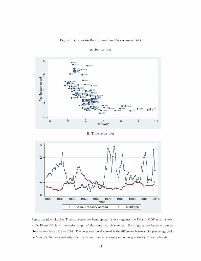
Figure 1: Corporate Bond Spread and Government Debt
A. Scatter plot
19191920
192119221923
1924
19251926
19271928
1929
19301931
1932
1933
1934
1935
1936
1937
1938 1939
1940
1941
1942
1943 19441945
19461947
19481949
195019511952
1953
1954
1955
1956
1957
19581959
19601961
1962
196319641965
1966
1967
1968
1969
1970
1971
1972
1973
1974
1975
1976
1977
1978
1979
1980
1981
1982
1983
1984
1985
1986
1987
1988
1989
1990
19911992
1993
1994
1995
1996
1997
1998
1999
2000
2001
2002
2003
200420052006
2007
2008
0.5
11.
52
Aaa
−Tre
asur
y sp
read
0 .2 .4 .6 .8 1 1.2Debt/gdp
B. Time series plot
0.5
11.
52
1920 1930 1940 1950 1960 1970 1980 1990 2000 2010Year
Aaa−Treasury spread Debt/gdp
Figure 1A plots the Aaa-Treasury corporate bond spread (y-axis) against the Debt-to-GDP ratio (x-axis)
while Figure 1B is a time-series graph of the same two time series. Both figures are based on annual
observations from 1919 to 2008. The corporate bond spread is the difference between the percentage yield
on Moody’s Aaa long maturity bond index and the percentage yield on long maturity Treasury bonds.
47

Figure 2: Money and Government Debt
A. Scatter plot
1934
1935
1936
1937
1938
1939
1940
1941
1942
1943
1944
1945
194619471948
19491950
195119521953
195419551956
1957
195819591960
1961
1962
1963
1964
19651966
19671968
1969
1970
1971
19721973
1974
1975
1976
1977
1978
19791980
1981
1982
1983
19841985 19861987
198819891990
1991
1992
1993
199419951996
1997
19981999
2000
2001
2002
20032004
200520062007 2008
.2.3
.4.5
non−
M1M
2/gd
p
.2 .4 .6 .8 1 1.2Debt/gdp
B. Time series plot
.2.4
.6.8
11.
2
1930 1940 1950 1960 1970 1980 1990 2000 2010Year
non−M1M2/gdp Debt/gdp
Figure 2A plots the quantity of small time and savings deposits, measured as M2 minus M1 minus Treasury
holdings of retail money market funds divided by GDP, against the Debt-to-GDP ratio while Figure 2B is a
time-series graph of the same two time series. Both figures are based on annual observations from 1934 to
2008.
48

Table I
Impact of Treasury Supply on Bond Spreads: Log Specification
The dependent variables are short and long-term yield spreads between corporate and Treasury bonds, both measured in percentage units. Independent variablesare the log of the ratio of the market value of Treasury debt outstanding to US GDP, and controls for the default risk and risk premium on corporate bonds. EDFis the expected default frequency for corporate bonds. Volatility is the annualized standard deviation of weekly log stock returns on the S&P500 index. Slope isthe slope of the Treasury yield curve measured as the spread between the 10-year Treasury yield and the 3-month Treasury yield. The data appendix providesthe precise definitions of all variables. EDF, volatility, and slope controls are demeaned. Regressions are estimated by ordinary least squares. The standard errorsare adjusted assuming errors are AR(1). We use the Box-Jenkins methodology for identifying the error structure. ρ denotes the first order autocorrelation of theerror terms. t-statistics in brackets.
Panel A: Aaa-Treasury Panel B: Baa-Treasury Panel C: CP-Bills Panel D: CPP2-Bills
(1) (2) (3) (4) (5) (6) (7) (8) (9)
Period 1919-2008 1969-2007 1926-2008 1969-2007 1926-2008 1920-2008 1969-2007 1926-2008 1974-2007
log(Debt/GDP ) -0.744 -0.910 -0.797 -1.752 -1.304 -0.728 -1.006 -0.550 -1.919
[-4.32] [-3.35] [-5.06] [-5.98] [-7.54] [-4.37] [-2.21] [-3.52] [-3.86]
EDF 0.953 1.206 0.024 0.086
[3.57] [3.71] [0.05] [0.16]
V olatility 1.294 6.364 1.947
[1.90] [6.88] [2.33]
Slope 0.045 0.080 0.175 0.309 -0.123 -0.085 -0.105
[1.05] [1.86] [2.04] [4.64] [-1.30] [-1.42] [-1.13]
Intercept 0.111 0.052 0.078 0.208 0.737 0.095 -0.269 0.229 -0.813
[0.62] [0.18] [0.49] [0.66] [4.34] [0.56] [-0.55] [1.49] [-1.58]
R2 0.447 0.623 0.568 0.669 0.690 0.224 0.211 0.259 0.282
ρ 0.572 0.402 0.528 0.066 0.012 0.183 -0.023 0.018 0.122
N 90 39 83 39 83 89 39 83 34
49
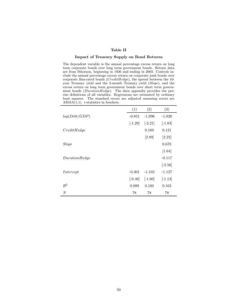
Table II
Impact of Treasury Supply on Bond Returns
The dependent variable is the annual percentage excess return on longterm corporate bonds over long term government bonds. Return dataare from Ibbotson, beginning in 1926 and ending in 2003. Controls in-clude the annual percentage excess return on corporate junk bonds overcorporate Baa-rated bonds (CreditHedge), the spread between the 10-year Treasury yield and the 3-month Treasury yield (Slope), and theexcess return on long term government bonds over short term govern-ment bonds (DurationHedge). The data appendix provides the pre-cise definitions of all variables. Regressions are estimated by ordinaryleast squares. The standard errors are adjusted assuming errors areARMA(1,1). t-statistics in brackets.
(1) (2) (3)
log(Debt/GDP ) -0.851 -1.696 -1.826
[-1.29] [-2.21] [-1.83]
CreditHedge 0.160 0.121
[2.89] [2.22]
Slope 0.678
[1.64]
DurationHedge -0.117
[-2.56]
Intercept -0.301 -1.245 -1.127
[-0.46] [-1.60] [-1.13]
R2 0.009 0.100 0.162
N 78 78 78
50

Table III
Impact of Treasury Supply on the Price of Safety and the Price of Liquidity
The dependent variables are: The spread between Baa-rated corporate bonds and Aaa-rated bonds (column (1) and (2)), the spread between A2/P2-rated andA1/P1-rated commercial paper (column (3) and (4)), the spread between the interest rate on FDIC insured 6 month CDs and 6-month Treasury bills (column (5)),and the spread between the average interest rate paid by banks on time and savings deposits and 6-month Treasury bills (column (6)). Independent variables are thelog of the ratio of the market value of Treasury debt outstanding to US GDP, the log of the ratio of the market value of Treasury debt with remaining maturity greaterthan 10 years to US GDP, the log of the ratio of the market value of Treasury debt with remaining maturity less than 1 year to US GDP, the annualized standarddeviation of weekly log stock returns on the S&P500 index (V olatility), and the slope of the Treasury yield curve measured as the spread between the 10-year Treasuryyield and the 3-month Treasury yield in column (1)-(4) and as the spread between the 10-year Treasury yield and the 6-month Treasury yield in column (5)-(6). Thedata appendix provides the precise definitions of all variables. Regressions are estimated by ordinary least squares or instrumental variables (2SLS), where we useinstruments Debt/GDP , (Debt/GDP )2, and (Debt/GDP )3, as indicated. The standard errors are adjusted assuming errors are AR(1) or i.i.d. as indicated. We usethe Box-Jenkins methodology for identifying the error structure. t-statistics in brackets.
Panel A: Price of Safety Panel B: Price of Liquidity
Assets with similar liquidity and different safety: Assets with similar safety and different liquidity:
SBaa−Aaa SP2−P1 SFDIC insured CDs-Bills STime & Savings Accounts-Bills
(1) (2) (3) (4) (5) (6)
Period 1926-2008 1926-2008 1974-2007 1974-2007 1984-2008 1935-1965
log(Debt/GDP ) -0.506 -0.879 -1.904 -0.639
[-3.42] [-4.47] [-1.83] [-2.37]
log(Debt > 10 year mat/GDP), instr. by -0.310
(Debt/GDP), (Debt/GDP)2, (Debt/GDP)3 [-2.40]
log(Debt ≤ 1 year mat/GDP) instr. by -1.453
(Debt/GDP), Debt/GDP)2, (Debt/GDP)3 [-2.94]
V olatility 5.070 6.311 0.321 0.029
[6.53] [6.66] [0.38] [0.03]
Slope 0.229 0.209 0.014 0.054 0.137 1.013
[4.15] [3.24] [0.40] [1.14] [1.32] [8.48]
Constant 0.660 0.241 -0.500 -2.662 -1.500 -0.070
[4.52] [0.648] [-2.45] [-2.56] [-1.63] [-0.41]
N 83 83 34 34 25 31
R2 0.600 0.486 0.271 0.720
Estimation method OLS IV OLS IV OLS OLS
Error term AR(1) AR(1) AR(1) AR(1) i.i.d. i.i.d.
51

Table IV
Demand Curve Estimate of Long-term Holders
The dependent variable is the spread between Baa bonds and Aaa bonds. The independent variables are thelog of the ratio of the Treasury holdings of public and private pension funds and insurance companies to GDP(log(DebtGROUP /GDP )), the annualized standard deviation of weekly log stock returns on the S&P500 index(V olatility), and the slope of the Treasury yield curve measured as the spread between the 10-year Treasury yield andthe 6-month Treasury yield (Slope). The data appendix provides the precise definitions of all variables. The estima-tion is by instrumental variables (2SLS), where we use instruments Debt/GDP , (Debt/GDP )2, and (Debt/GDP )3.Standard errors are adjusted assuming an AR(2) error structure. t-statistics in brackets.
Period log(DebtGROUP /GDP ) V olatility Slope Constant N
1945-2008 -0.372 [-1.95] 3.484 [2.56] 0.207 [3.35] -0.266 [-0.44] 64
52

Table V
Response of Money to Treasury Supply, 1934-2008
Panel A presents reduced form regressions between measures of money and Treasury supply. The money measures include small time and savings depositsand non-Treasury retail money market fund holdings (non-M1 M2, minus retail money market fund Treasury holdings) and small and large time andsavings deposits, non-Treasury retail and institutional money market fund holdings, repos and Eurodollars (non-M1 M3, minus retail and institutionalmoney market fund Treasury holdings). Panel B presents structural instrumental variables estimates of the supply response of the banking system. Inthe first stage, the spread between Baa bond yields and the interest rate on non-M1 M2 is regressed on log(Debt/GDP ) and controls. In the secondstage, log(non − M1M2/GDP ) is regressed on the fitted values of the spread and controls. The data appendix provides the precise definitions of allvariables. The regressions in Panel B exclude the Regulation Q period of 1966-1983. Errors are adjusted assuming serial correlation of either AR(2) orAR(1), as indicated. We use the Box-Jenkins methodology to identify the error structure. t-statistics in brackets.
Panel A: Reduced Form Panel B: Structural Form
(1) (2) (3) (4) (5)
1st Stage of IV 2nd Stage of IV
Dep. Var. non-M1 M2/GDP non-M1 M2/GDP non-M1 M3/GDP SBaa−(non−M1M2) log(non − M1M2/GDP )
Period 1926-2008 1959-2005 1959-2005 1935-1965, 1935-1965,
1984-2008 1984-2008
Debt/GDP -0.305 -0.352 -0.553 Log(Debt/gdp) -1.587 SBaa−nonM1M2 0.394
[-5.52] [-4.16] [-3.34] [-2.10] [2.29]
Y ear 0.001 0.007 V olatility 7.942 V olatility -2.717
[1.86] [5.99] [2.81] [-1.47]
Slope 0.440 Slope -0.140
[2.27] [-1.37]
Intercept 0.502 -1.467 -12.161 Intercept 2.279 Intercept -2.439
[18.26] [-1.38] [-5.69] [3.94] [-4.13]
R2 0.601 0.534 0.802
N 75 47 47 56 56
Estimation method OLS OLS OLS OLS IV
Standard errors AR(2) AR(2) AR(2) AR(1) AR(1)
53
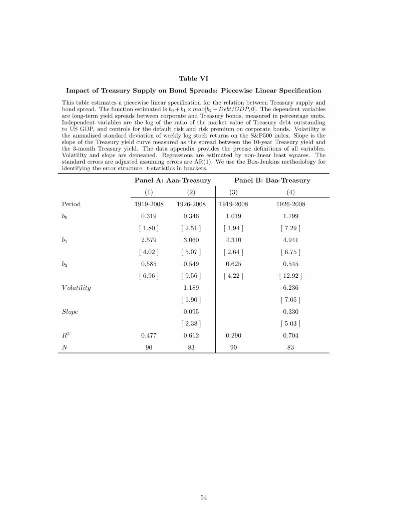
Table VI
Impact of Treasury Supply on Bond Spreads: Piecewise Linear Specification
This table estimates a piecewise linear specification for the relation between Treasury supply andbond spread. The function estimated is b0 + b1 ×max[b2−Debt/GDP,0]. The dependent variablesare long-term yield spreads between corporate and Treasury bonds, measured in percentage units.Independent variables are the log of the ratio of the market value of Treasury debt outstandingto US GDP, and controls for the default risk and risk premium on corporate bonds. Volatility isthe annualized standard deviation of weekly log stock returns on the S&P500 index. Slope is theslope of the Treasury yield curve measured as the spread between the 10-year Treasury yield andthe 3-month Treasury yield. The data appendix provides the precise definitions of all variables.Volatility and slope are demeaned. Regressions are estimated by non-linear least squares. Thestandard errors are adjusted assuming errors are AR(1). We use the Box-Jenkins methodology foridentifying the error structure. t-statistics in brackets.
Panel A: Aaa-Treasury Panel B: Baa-Treasury
(1) (2) (3) (4)
Period 1919-2008 1926-2008 1919-2008 1926-2008
b0 0.319 0.346 1.019 1.199
[ 1.80 ] [ 2.51 ] [ 1.94 ] [ 7.29 ]
b1 2.579 3.060 4.310 4.941
[ 4.02 ] [ 5.07 ] [ 2.64 ] [ 6.75 ]
b2 0.585 0.549 0.625 0.545
[ 6.96 ] [ 9.56 ] [ 4.22 ] [ 12.92 ]
V olatility 1.189 6.236
[ 1.90 ] [ 7.05 ]
Slope 0.095 0.330
[ 2.38 ] [ 5.03 ]
R2 0.477 0.612 0.290 0.704
N 90 83 90 83
54

Table VII
Debt Holdings, by Group
Panel A of this table presents statistics on the fraction of Treasury securities held by various groups. PanelB presents the bond portfolio composition of each of the groups, broken down into Treasury, Agency, andshort and long-term corporate bonds. The data are from the Flow of Funds Accounts of the Federal Reserve,and are annual (end of year) from 1945 to 2008. Mutual funds include closed-end funds and exchange tradedfunds.
Group Panel A: Who Holds Treasury Debt?
Mean Std. Dev. 1945 1975 2008
Federal Reserve Banks 0.138 0.040 0.097 0.199 0.075
Foreign Official Holdings 0.113 0.088 0.010 0.141 0.367
State/Local Governments 0.088 0.042 0.022 0.064 0.076
Banks/Credit Institutions 0.201 0.116 0.416 0.222 0.017
Households and Mutual Funds 0.260 0.051 0.265 0.263 0.169
Foreign Private Sector 0.042 0.049 0.000 0.010 0.140
Fedrl/State/Local Govt. Ret. 0.035 0.022 0.006 0.006 0.045
Private Pensions 0.028 0.020 0.008 0.029 0.029
Insurance Companies 0.048 0.023 0.093 0.022 0.025
Panel B: Bond Market Portfolio Composition
Treasury Agency Long-term Short-term
Corporate Corporate
Federal Reserve Banks 0.983 0.017 0.000 0.001
Foreign Official Holdings 0.948 0.052 0.000 0.000
State/Local Governments 0.720 0.217 0.029 0.034
Banks/Credit Institutions 0.526 0.312 0.141 0.020
Households and Mutual Funds 0.563 0.095 0.223 0.118
Foreign Private Sector 0.240 0.084 0.479 0.197
Fedrl/State/Local Govt. Ret. 0.387 0.108 0.487 0.018
Private Pensions 0.233 0.142 0.583 0.042
Insurance Companies 0.172 0.078 0.726 0.024
55
Recommended